


1. Introduction
The worldwide installed capacity of offshore wind has been significantly growing since 2010. Most current offshore wind turbines are mounted on fixed structures and clustered in wind farms installed in water depths less than 60 m (Díaz & Soares Reference Díaz and Soares2020). For water depths greater than 60 m, a floating wind turbine is the preferred solution (Hannon et al. Reference Hannon, Topham, Dixon, McMillan and Collu2019). Compared with a fixed turbine, a floating offshore wind turbine (FOWT) is free to move in its six degrees-of-freedom (DoF). The action of wind, waves and current is responsible for complex platform motions (Jonkman & Matha Reference Jonkman and Matha2011). These motions depend, among others, on platform types, environmental conditions, moorings and water depth (Butterfield et al. Reference Butterfield, Musial, Jonkman and Sclavounos2007; Goupee et al. Reference Goupee, Koo, Kimball, Lambrakos and Dagher2014). The effect of the motions on rotor aerodynamics is an active research topic that is becoming highly relevant. As turbines are usually installed in wind farm configurations, wake development is of particular interest, for example, for wind farm control strategies, power optimisations, etc.
Typical distances between offshore turbines within a farm in the main direction of the wind are in the range of 6 to 12 $D$ (with $D$ the rotor diameter) (Hou et al. Reference Hou, Zhu, Ma, Yang, Hu and Chen2019). This implies that downstream turbines operate in the wake of upstream turbines. The wake of an offshore turbine is a high-turbulent and low-energy flow region compared with the undisturbed flow. There is thus much interest in understanding the evolution of the wake of a wind turbine and especially the features of the far-wake (typically for $x/D \geq 6$). Over the past decades, several numerical studies, theoretical models, field measurements and wind tunnel experiments have been carried out, leading to significant progress in the rich subject of fixed wind turbine wakes, see for example Ainslie (Reference Ainslie1988), Vermeer, Sørensen & Crespo (Reference Vermeer, Sørensen and Crespo2003), Chamorro & Porté-Agel (Reference Chamorro and Porté-Agel2009), Porté-Agel, Bastankhah & Shamsoddin (Reference Porté-Agel, Bastankhah and Shamsoddin2020) and Neunaber et al. (Reference Neunaber, Hölling, Stevens, Schepers and Peinke2020).
(i) Wake regions of a fixed wind turbine. As the study of the wake of a FOWT assumes a good knowledge of the wake of a fixed wind turbine, we start with a discussion on this subject. The near-wake is located in the vicinity of the turbine (usually  $x<4D$), characterised by the presence of hub-, root- and tip-vortices (Vermeer et al. Reference Vermeer, Sørensen and Crespo2003; Neunaber et al. Reference Neunaber, Hölling, Stevens, Schepers and Peinke2020). The flow in this region displays homogenous decaying turbulence. The coherent structures (tip-vortices, etc.) are carried downstream by the flow until instabilities occur, eventually leading to their destruction (Widnall Reference Widnall1972; Felli, Camussi & Di Felice Reference Felli, Camussi and Di Felice2011; Lignarolo et al. Reference Lignarolo, Ragni, Scarano, Ferreira and Van Bussel2015). Among these, mutual inductance is of great importance, particularly for low-turbulence inflows; as they move downstream, helical vortices are affected by neighbouring vortices and interact with each other until they break up. For flows with high turbulence, mutual inductance may not be the main factor in the breakup of helical vortices (Hodgkin, Deskos & Laizet Reference Hodgkin, Deskos and Laizet2023). In the near-wake, it was shown by Lignarolo et al. (Reference Lignarolo, Ragni, Scarano, Ferreira and Van Bussel2015) that the tip-vortices shield the wake from the outer flow and prevent the exchange of momentum that provides re-energisation to the wake, as predicted by Medici (Reference Medici2005). The recovery process thus starts when the tip vortices become unstable, which marks the beginning of the transition region. From there, the shear layer (highly turbulent region), which separates the wake from the undisturbed flow, grows radially. Momentum is transported from the outer region to the wake, and turbulence builds up. Farther downstream, the shear layers merge at the centre. Here, the amount of turbulence in the wake is at its maximum and then gradually decreases as it moves downstream (similar to the behaviour of the wake of a fractal grid as shown by Hurst & Vassilicos (Reference Hurst and Vassilicos2007)). Around this position, the wind speed along the centre line begins to recover, indicating the start of the far-wake, which features a characteristic Gaussian wind deficit profile. The far-wake can be separated into a decay region and a fully developed far-wake when turbulence has reached a homogeneous-isotropic state (Pope Reference Pope2000). The size of each region, the intensity of the recovery and the turbulence of the wake depend greatly on the type of inflow and the operating conditions of the turbine (Wu & Porté-Agel Reference Wu and Porté-Agel2012; Iungo, Wu & Porté-Agel Reference Iungo, Wu and Porté-Agel2013; Neunaber et al. Reference Neunaber, Schottler, Peinke and Hölling2017; Gambuzza & Ganapathisubramani Reference Gambuzza and Ganapathisubramani2023). It is clear that the emergence of the far-wake is directly linked to the phenomena that happen closer to the rotor; however, in the far-wake, the detailed features of its turbulence appear to be universal (Ali et al. Reference Ali, Fuchs, Neunaber, Peinke and Cal2019).
(ii) Wake meandering of a fixed wind turbine. An important property of the wake of a wind turbine is its tendency to oscillate side-to-side and up and down, so-called wake meandering (Medici & Alfredsson Reference Medici and Alfredsson2006; Larsen et al. Reference Larsen, Madsen, Thomsen and Larsen2008; Howard et al. Reference Howard, Singh, Sotiropoulos and Guala2015). This phenomenon originates from two different causes. On the one hand, the turbulent flow of the atmosphere contains large eddies whose scale is larger than the wake width. These large eddies pass through the rotor and are responsible for the wake's low frequency and large amplitude oscillation (Larsen et al. Reference Larsen, Madsen, Thomsen and Larsen2008; Espana et al. Reference Espana, Aubrun, Loyer and Devinant2011; Heisel, Hong & Guala Reference Heisel, Hong and Guala2018).
On the other hand, wake instabilities can cause meandering in the far-wake, where the wake tends to oscillate within a range of frequencies, expressed in terms of a meandering Strouhal number,  $St_m = f_m D/U_{\infty } \in [0.1, 0.5]$. This phenomenon is more likely to occur when the inflow's turbulence intensity is low, i.e. $TI_{\infty } \leq 0.05$. Observations from various studies, such as Okulov et al. (Reference Okulov, Naumov, Mikkelsen, Kabardin and Sørensen2014), Foti, Yang & Sotiropoulos (Reference Foti, Yang and Sotiropoulos2018), Heisel et al. (Reference Heisel, Hong and Guala2018) and Gupta & Wan (Reference Gupta and Wan2019), have revealed a broad peak in the spectrum around $St_m$, indicating that wake oscillations differ from classical vortex shedding, which typically exhibits a sharp peak at the shedding frequency. It is, therefore, inappropriate to define a particular meandering frequency but rather a range of frequencies. After Gupta & Wan (Reference Gupta and Wan2019), wake meandering occurs in the far wake due to the ‘amplification of upstream disturbances by shear flow instabilities’, a phenomenon also observed by Gambuzza & Ganapathisubramani (Reference Gambuzza and Ganapathisubramani2023). Periodic excitation in the range of $St_m$, where wake meandering naturally occurs, can lead to an early onset of meandering (Mao & Sørensen Reference Mao and Sørensen2018; Gupta & Wan Reference Gupta and Wan2019; Hodgson, Madsen & Andersen Reference Hodgson, Madsen and Andersen2023). Following this idea, some control strategies, such as the helix approach (a blade pitching control method), trigger instabilities that lead to the formation of large coherent structures in the wake (Frederik et al. Reference Frederik, Doekemeijer, Mulders and van Wingerden2020; Korb, Asmuth & Ivanell Reference Korb, Asmuth and Ivanell2023). This strategy enables a faster transition to far-wake and a more efficient wake mixing, i.e. a faster wake recovery.
(iii) Wake of a floating wind turbine. The latest topic of floating wind turbines raises fundamental questions about the impact of rotor movements on the development of the wake. Another aspect not further discussed here is the impact on rotor aerodynamics. Firstly, the motions of a floating turbine are responsible for unsteady aerodynamic phenomena. Unsteadinesses are observed for high-frequency motions, characterised by the dimensionless Strouhal number,  $St = f_p D / U_{\infty }$ (where $f_p$ is the frequency of motion, $D$ is the rotor diameter and $U_{\infty }$ is the inflow speed), typically for $St > 0.5$ (Sebastian & Lackner Reference Sebastian and Lackner2013; Farrugia, Sant & Micallef Reference Farrugia, Sant and Micallef2014; Sant et al. Reference Sant, Bonnici, Farrugia and Micallef2015; Bayati et al. Reference Bayati, Belloli, Bernini and Zasso2017a; Fontanella et al. Reference Fontanella, Bayati, Mikkelsen, Belloli and Zasso2021). Secondly, the wake generated by a floating wind turbine is impacted by the different motions, which was shown through various wind tunnel studies with model turbines and porous disks (Rockel et al. Reference Rockel, Camp, Schmidt, Peinke, Cal and Hölling2014, Reference Rockel, Peinke, Hölling and Cal2017; Bayati et al. Reference Bayati, Belloli, Bernini and Zasso2017b; Fu et al. Reference Fu, Jin, Zheng and Chamorro2019; Kopperstad, Kumar & Shoele Reference Kopperstad, Kumar and Shoele2020; Schliffke, Aubrun & Conan Reference Schliffke, Aubrun and Conan2020; Belvasi et al. Reference Belvasi, Conan, Schliffke, Perret, Desmond, Murphy and Aubrun2022; Fontanella, Zasso & Belloli Reference Fontanella, Zasso and Belloli2022; Meng et al. Reference Meng, Su, Qu and Lei2022).
Bayati et al. (Reference Bayati, Belloli, Bernini and Zasso2017b) discussed the relevance of the so-called ‘wake reduced velocity’, equivalent to a Strouhal number, for characterising unsteady aerodynamic conditions. Fu et al. (Reference Fu, Jin, Zheng and Chamorro2019) measured with particle image velocimetry the wake of a pitching and rolling model turbine with relatively high amplitudes (up to  $20^{\circ }$) and low frequencies ( $St < 0.03$). They observed a higher recovery for the floating turbine and enhanced turbulent kinetic energy, which Rockel et al. (Reference Rockel, Peinke, Hölling and Cal2017) also observed. Schliffke et al. (Reference Schliffke, Aubrun and Conan2020) carried out a more systematic study in which they measured at 4.6D downstream the wake of a surging porous disc with $St \in [0, 0.24]$ under realistic turbulent conditions. No impact of motions on the recovery of the wake was measured. However, a signature of the motions in the spectra of the wake was observed for all frequencies. Kopperstad et al. (Reference Kopperstad, Kumar and Shoele2020) investigated in a wind tunnel and with computational fluid dynamics (CFD) the wake of a spar and barge floating turbine. They showed that a floating turbine's wake recovers faster than a fixed turbine in a laminar wind. Also, the recovery depends on the wave excitation.
Numerical simulations using free-wake vortex code and CFD were carried out to study the different wake regions of a floating turbine (Farrugia, Sant & Micallef Reference Farrugia, Sant and Micallef2016; Lee & Lee Reference Lee and Lee2019; Chen, Liang & Li Reference Chen, Liang and Li2022; Kleine et al. Reference Kleine, Franceschini, Carmo, Hanifi and Henningson2022; Li, Dong & Yang Reference Li, Dong and Yang2022; Ramos-García et al. Reference Ramos-García, Kontos, Pegalajar-Jurado, González Horcas and Bredmose2022). Farrugia et al. (Reference Farrugia, Sant and Micallef2016) outlined the possibility for surge motion ‘to induce the onset of complex interactions between adjacent tip vortices’. These instabilities induced by surge motion on the complex helical vortex system could explain the faster recovery of the wake of a surging turbine for a range of  $St\in [0.4, 1.7]$, studied by Ramos-García et al. (Reference Ramos-García, Kontos, Pegalajar-Jurado, González Horcas and Bredmose2022). Based on the stability theory of vortices, Kleine et al. (Reference Kleine, Franceschini, Carmo, Hanifi and Henningson2022) showed that the motion of a floating turbine ‘excites vortex instabilities modes’, which were predicted by Farrugia et al. (Reference Farrugia, Sant and Micallef2016). They showed that disturbances at frequencies of $0.5$ and $1.5$ times the rotor's 1P frequency produce the most significant disruptions. Chen et al. (Reference Chen, Liang and Li2022) carried out CFD simulations of the wake of a surging turbine with amplitude $A_p \in [0.03D, 0.1D]$, and frequency $St \in [0.41, 1.64]$. They showed the positive impact of motions on the recovery of the wake of a surging turbine, where up to 10 % more recovery compared with the fixed turbine was found. Last but not least, Li et al. (Reference Li, Dong and Yang2022) used CFD to study the onset of wake meandering arising from the sideways motion of a floating turbine. They demonstrated that sway motion for $St \in [0.2, 0.6]$ helps the wake to recover up to 25 % more compared with the fixed case. They showed that side-to-side turbine motions lead to large wake meandering, even with small amplitude of motions ( $A_p/D \approx 0.01$). This important result is particularly pronounced for low turbulent conditions ( $TI_{\infty } < 0.05$). In a wind farm configuration, wake oscillations can increase the movement of downstream floating wind turbines (Wise & Bachynski Reference Wise and Bachynski2020).
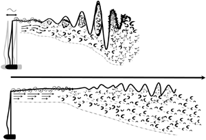
The discussion mentioned above shows that the current understanding of the wake of floating wind turbines is based on many specific investigations. It remains unclear which frequency range and type of motion influence the wake generated by a FOWT. Moreover, the effects on wake dynamics are not yet sufficiently understood. The lack of systematic studies in this area limits the ability to draw general conclusions. The papers published so far have focused mainly on cases of high turbulence ( $TI_{\infty } > 0.08$) where the effect of the motions is mixed with the effect of the turbulence, which makes the problem particularly complex. In Pimenta et al. (Reference Pimenta2021), we reported on pp. 4–5 on wind tunnel experiments that we conducted in 2021 on cases similar to Li et al. (Reference Li, Dong and Yang2022). In this paper, we extended our experiments to side-to-side and fore–aft harmonic motions (see figure 1 for the different DoFs) to obtain a more global understanding of the wake development of a FOWT. A particular focus was given to the influence of the frequency of movements. In order to examine solely the impact of the motion on the wake and to exclude any impact of inflow turbulence, the turbine was operated in laminar wind.

Figure 1. (a) Fore–aft (surge and pitch) and (b) side-to-side motions (sway and roll) of a FOWT.
This simplification to laminar inflow conditions was made in order to reduce the complex environment of a FOWT, necessary to gain a more fundamental understanding of the wake dynamics of this new type of wind turbine. Our work focuses on analysing the impact of a periodic motion on wake recovery and studying underlying mechanisms affecting the recovery. We discovered rich nonlinear dynamics in the wake, which are driven by the motions of the platform. We believe these results are of interest not only in the context of wind energy but also for fluid mechanics of turbulent wakes in general, with a new insight on the transition to far-wake in high  $Re$ flow ( $Re > 10^5$) periodically excited.
Section 2 details the experimental set-up and the cases investigated. Section 3 presents the averaged results, i.e. the profiles of wake deficit and turbulence intensity. Here, we show the dependency on the DoF on the wake. We describe the effects of side-to-side motions with  $St \in [0, 0.58]$ and fore–aft motions with $St \in [0, 0.97]$ on wake recovery. We identify two regions in the wake corresponding roughly to the transition region and the far-wake (see (i) above). Section 4 first examines the dynamics of the far-wake (for $x \geq 6D$) and discusses the results regarding nonlinear dynamics. Section 5 then focuses on the development of wake dynamics in the shear layer for $x \geq 3D$ (i.e. in the transition region). Section 6 finally brings together the recovery results with the nonlinear dynamics. We finish by discussing the transition to far-wake in a broader context.
2. Experiments
2.1. Set-up
The experimental set-up used to perform the investigations is illustrated in figure 2. The experiments were done in the  $3\,{\rm m} \times 3\,{\rm m} \times 30\,{\rm m}$ test section of the large wind tunnel of the University of Oldenburg (Kröger et al. Reference Kröger, Frederik, van Wingerden, Peinke and Hölling2018). The set-up consists of the Model Wind Turbine Oldenburg 0.6 (MoWiTO 0.6) with a diameter of 0.58 m mounted on a six-DoF motorised platform, designed specifically for the MoWiTO 0.6 (Messmer et al. Reference Messmer, Brigden, Peinke and Hölling2022). With this system, the model turbine can be moved following predefined motion signals in the six-DoF: the three translations – surge, sway and heave; and the three rotations – roll, pitch and yaw. In this paper, we use the terminology ‘floating wind turbine’ to describe our experimental set-up, despite the fact that we consider idealised conditions (harmonic motion and laminar wind).

Figure 2. Scheme of the experimental set-up, the MoWiTO 0.6 mounted on a six-DoF platform installed in the wind tunnel (a) side view and (b) front view. The figure is not to scale.
The model turbine was equipped with a strain gauge to measure the thrust,  $T$, of the ensemble (tower and rotor). For any case investigated, power produced, rotational speed and thrust of the turbine were recorded. The movements of the platform were recorded to verify the adequacy of the motions. The streamwise wind speed, $U$, was measured with an array of 19 one-dimensional hot-wires of ${\sim }$1 mm length, resolving turbulent scale of this size.
The probes were operated with multichannel constant temperature anemometer (54N80-CTA) modules from Dantec Dynamics. Data were acquired with a sampling rate of 6 kHz, gathering around  $10^6$ points for each measurement. The time of measurements, $T_{meas}$, was sufficient to reach statistical convergence of any postprocessed data shown and discussed in this paper. The hot-wire probes were calibrated twice daily, and temperature, humidity and air pressure were recorded throughout the day to track any drift effects, which turned out to be negligible. The inflow wind speed was measured with a Prandtl-tube approximately 2 m in front of the model turbine.
The array was mounted on a moving motorised cart, which allowed us to measure the wind speed at a downstream position,  $x$, from 1.5D to 12D (cf. figure 2a). The hot-wires were placed on a horizontal line at hub height (around 1 m above floor level) and span lateral positions, $y$ from $-2.5R$ to $2.5R$ ( $R = D/2$) with respect to the hub centre (cf. figure 2b).
2.2. The MoWiTO 0.6
The MoWiTO 0.6 used for the experiments has a rotor diameter  $D$ of 0.58 m. The turbine was developed at the University of Oldenburg (Schottler et al. Reference Schottler, Hölling, Peinke and Hölling2016; Jüchter et al. Reference Jüchter, Peinke, Lukassen and Hölling2022). The properties of the turbine are depicted in table 1. The model turbine was used for several measurement campaigns with a focus on wake flow; further details of the experimental procedure and wake measurements can be found in Hulsman et al. (Reference Hulsman, Wosnik, Petrović, Hölling and Kühn2020), Neunaber et al. (Reference Neunaber, Hölling, Stevens, Schepers and Peinke2020) and Neunaber, Hölling & Obligado (Reference Neunaber, Hölling and Obligado2024).
Table 1. The MoWiTO 0.6 characteristics.

For the experiments, we used wind speeds between 3 and 5 m s $^{-1}$. We fixed the tip speed ratio for all cases so that $\langle TSR\rangle = 6 \pm 0.1$. We operated the turbine at a constant blade pitch angle, around the optimum, which gives $\langle C_T \rangle = 0.86 \pm 0.05$ for $U_{\infty } = 3\,{\rm m}\,{\rm s}^{-1}$ and $\langle C_T \rangle = 0.81 \pm 0.05$ for $U_{\infty } = 5\,{\rm m}\,{\rm s}^{-1}$. The thrust coefficient account for rotor and tower aerodynamic loads (in a previous study by Neunaber et al. (Reference Neunaber, Hölling, Stevens, Schepers and Peinke2020), the load on the tower and nacelle without the blades of the MoWiTO 0.6 was measured to be 17 % of the total thrust coefficient). The power performance of the turbine depends on $Re$, we measured $\langle C_p \rangle = 0.21 \pm 0.01$ at $U_{\infty } = 3\,{\rm m}\,{\rm s}^{-1}$ and $\langle C_p \rangle = 0.3 \pm 0.01$ at $U_{\infty } = 5\,{\rm m}\,{\rm s}^{-1}$.
2.3. Non-dimensional parameters that drive the wake behaviour
Our experimental research involves numerous quantities. We briefly discuss the selection of necessary parameters for a complete characterisation. Therefore, we use the basis of the  ${\rm \pi}$-theorem. For a given DoF, the system investigated involves nine independent parameters: platform motion frequency and amplitude; inflow wind speed; rotor diameter; air viscosity; air density; turbine thrust and power; and rotational speed. These are noted as $f_p$, $A_p$, $U_{\infty }$, $D$,
$D$,  $\mu$, $\rho$, $T$,
$T$,  $P$,
$P$,  $\omega$. The ${\rm \pi}$-theorem suggests that, a problem characterised by $m$ dimensional variables can always be reduced to a set of $m-n$ dimensionless parameters ( ${\rm \pi}$-groups), with $n$ the fundamental units of measure (dimensions) as depicted by Buckingham (Reference Buckingham1914). Therefore, this problem with nine variables and three dimensions can be reduced to six dimensionless parameters. These are all defined in table 2, namely the thrust coefficient, $C_T$, power coefficient, $C_P$, tip speed ratio, $TSR$, reduced amplitude, $A^*$, Strouhal number, $St$, and Reynolds number, ${\textit {Re}}$. Thus, in a laminar flow, the properties of the wake of a FOWT, $wake_{FOWT}$, are determined by these six dimensionless numbers: $wake_{FOWT} = f(C_T,C_P,TSR, A^*,St,Re)$.
Table 2. Dimensionless parameters that drive the wake of a FOWT.

The dependency on  $C_T$ of wake recovery and expansion of a wind turbine wake was characterised extensively (Porté-Agel et al. Reference Porté-Agel, Bastankhah and Shamsoddin2020). The tip speed ratio also plays an important role in the development of the wake of a FOWT (Farrugia et al. Reference Farrugia, Sant and Micallef2016). Both the amplitude and frequency of motions can impact the wake of a moving turbine, as demonstrated by Chen et al. (Reference Chen, Liang and Li2022), Li et al. (Reference Li, Dong and Yang2022) and Ramos-García et al. (Reference Ramos-García, Kontos, Pegalajar-Jurado, González Horcas and Bredmose2022). As mentioned above, motion frequency has a greater influence on wake dynamics, even at low amplitudes ( $A_p \sim 0.01D$). Based on these works and the set of parameters, we concluded that it is worth focusing on the impact of different $St$ values at a small amplitude of motions.
2.4. Cases investigated
Floating offshore wind turbines operate in the atmospheric boundary layer, which exhibits various turbulent conditions. Usually, the turbulence intensity in free flow,  $TI_{\infty }$, is found in $[0.02, 0.15]$. (Jacobsen & Godvik Reference Jacobsen and Godvik2021; Angelou, Mann & Dubreuil-Boisclair Reference Angelou, Mann and Dubreuil-Boisclair2023). In our experiments, we used idealised conditions (laminar wind with $TI_{\infty } \approx 0.003$ and one-DoF harmonic motions). We also carried out experiments with $TI_{\infty } = 0.03$ and observed similar results as the ones shown and discussed in this paper. Our study investigates the following DoFs: surge; sway; roll; pitch (see figure 1). We examined these DoFs independently, without combining them. We imposed the following motion signal on the platform, $\xi$, for a given DoF: $\xi (t) = A_p \sin (2 {\rm \pi}f_p t) = A^*D \sin (2 {\rm \pi}(St U_{\infty }/D) t)$. Here, $A_p$ denotes the amplitude of motion (in m or $^{\circ }$), and $f_p$ represents the frequency of motion (in Hz).
In order to investigate a relevant range of  $St$, we looked at the typical movements of a FOWT, which we briefly present below. The motions of a floating wind turbine are greatly influenced by the type of foundation used (tension-leg platform, semisubmersible, barge or spar). Three distinct ranges of frequencies are usually observed in the motion spectra of a floating turbine.
(i) Wave frequency. A floating platform is subject to ocean waves, which cause motions at frequencies around 0.1 Hz (wave period around 10 s). Although the wave-induced motions are rather low in amplitude ( $A^* \sim 0.01$), they are high in frequency. For a 10 MW turbine at rated wind speed, this type of motion typically gives $St \sim 1.5$ (Messmer et al. Reference Messmer, Brigden, Peinke and Hölling2022).
(ii) Rotational natural frequency. When a floating turbine is displaced from its equilibrium position (due to a gust or a series of waves), it goes back to equilibrium as a damped harmonic oscillator at a frequency that depends on the DoF. For a spar or a semisubmersible, the pitch and roll natural frequencies are typically around 0.035 Hz (Robertson et al. Reference Robertson, Jonkman, Masciola, Song, Goupee, Coulling and Luan2014). For a 10 MW turbine at rated wind speed, such motions give
$St \sim 0.5$ and $A^*$ up to $\sim 0.04$.(iii) Translation natural frequency. As with rotational DoF, a floating turbine undergoes translational movements at its natural frequencies. These can be large in amplitude (
$A^*$ up to ${\sim }0.1$) but at low frequency ( $f_p \sim 0.01$ Hz). A typical Strouhal number is $St \sim 0.1$ (Leimeister, Kolios & Collu Reference Leimeister, Kolios and Collu2018).


This discussion shows that, typically, the motions of floating turbines cover a range of Strouhal numbers,  $St \in [0, 1.5]$. While high-frequency movements are relatively low in amplitude ( $A^* \sim 0.01$), oscillations at lower frequencies can reach amplitudes up to 10 % of the rotor diameter. To test a wide range of $St$, we conducted experiments at frequencies ranging from $0.3$ to 5 Hz with low motion amplitudes. We covered $St \in [0, 0.97]$ (corresponding to the maximum operability range of the set-up). Table 3 details all the cases investigated in this paper.
Table 3. Motion cases investigated. For all cases,  $\langle TSR\rangle = 6.0 \pm 0.1$. For rotational DoFs: $A^* = T_{length} \times \tan (A_p)$ (see table 1).

To quantify the differences between the cases, we took as reference the fixed case ( $St = 0$). To make this study of our different cases comparable, it is essential to note that the mean power and thrust of the moving turbine were the same as those of the fixed turbine for a given wind speed. If this were not the case, comparing the wake flows between cases would be less meaningful, as there would be differences in mean operating conditions.
It was also confirmed by examining the wake deficit in the very near-wake ( $x \approx 1.5D$), which was the same for any case with the same $Re$,
$Re$,  $\langle C_T \rangle$, $\langle C_P \rangle$ and $\langle TSR \rangle$. With this, we concluded that the induction factor of the turbine was the same, which was also observed by Fontanella et al. (Reference Fontanella, Zasso and Belloli2022). In particular, such a result is not evident for fore–aft DoF as motions cause temporal variations in turbine power and thrust. We found that they do not affect the mean turbine output values, at least for such low amplitudes. However, the impact of the motions is directly related to their effects on the dynamics of the wake.
3. Results on average wake values
The scheme after which we present our results is briefly explained next. We consider four DoFs, for which we compare the wakes. The analysis is first done at three downstream positions ( $x \in [\kern-1pt[ 6D, 8D, 10D ]\kern-1pt]$) and then for $x \geq 3D$. The downstream dependence of the streamwise wake velocity deficit and turbulence intensity profiles, as well as wake recovery, is shown for different $St$. Appendix A describes the postprocessing methodology used.
We begin this section by presenting, in § 3.1, the similarity between DoF that led us to reduce the analysis to two generic DoFs, namely sway and surge. Second, the dependency of the wake recovery on the  $St$ is shown in § 3.2 for sway. Third, we present corresponding results for surge motions in § 3.3. Finally, we discuss in § 3.4 the results on wake recovery.
3.1. Equivalence between different DoF
In a previous study from Bayati et al. (Reference Bayati, Belloli, Bernini and Zasso2017a), the authors simplified the modelling of the aerodynamics of a FOWT by linearising rotational motions into translation. We checked whether this simplification also applies to the wake of a turbine with sway/roll motions or surge/pitch motions, respectively.
To address this issue, we measured the wake of the floating turbine with small ( $A_p = 0.5^{\circ }$) and large ( $A_p = 5^{\circ }$) amplitudes of platform roll around the zero value. Additionally, we performed tests with the turbine swaying at an equivalent amplitude. We carried out the same tests with pitch and surge DoFs (with no tilt angle). The results of side-to-side motions (sway and roll) are presented in figure 3, while the fore–aft motions are shown in Appendix B.

Figure 3. Wake deficit (a–c) and  $TI$ profiles (d–f) at 6D, 8D and 10D for fixed and two roll and sway cases with the same $St$ and $A^*$, ${\textit {Re}} = 2.3 \times 10^5$. Tests A.1–A.5 in table 3.
For the sway and roll cases, figure 3 demonstrates that the match of  $\Delta U / U_{\infty }$ and $TI$ is nearly perfect for the low amplitude ( $A^* = 0.007$) and the high amplitude ( $A^* = 0.065$). This suggests that the approximation made in Bayati et al. (Reference Bayati, Belloli, Bernini and Zasso2017a) can also be applied to the wake for these types of motions. We notice in figure 3(a–c) an asymmetry of the wake; the deficit is greater at $y = R$ than at $y = -R$, meaning the wake tends to deviate to the left. We attribute this phenomenon to a slight misalignment of the turbine with the incoming wind. For the lowest value of $Re$, we repeated the experiments by correcting the misalignment; as seen later the wake is more symmetric (this slight asymmetry has no significant influence on our results).
Our findings allowed us to simplify the study by focusing only on sway for side-to-side motion and surge for fore–aft motion. We can extend the conclusions of these DoFs to pitch and roll motions as long as the equivalent amplitude is below a specific value, which we estimate to be around  $2^{\circ }$, i.e. $A^* \approx 0.025$.
3.2. Sway motion
From the results presented in figure 3, we already see that the wake is strongly influenced by the frequency of the motion, i.e. by  $St$. We observed that the wake velocity profile is flatter with increasing frequency of motion. To investigate the $St$ dependency, we measured the wake for different platform motion frequencies at constant amplitude ( $A^* = 0.007$ and $St \in [0.12, 0.58]$) similar to the CFD simulations done by Li et al. (Reference Li, Dong and Yang2022).
Figure 4 shows the wake deficit and turbulence intensity profiles at 6D, 8D and 10D for the fixed and five sway cases. Most interestingly, we find that for  $St = 0.42$, the wake has the lowest deficit (figure 4b,c; green stars). Similar results are observed for the profiles of $TI$; see figure 4(e, f). Another interesting property of wakes, discussed by Porté-Agel et al. (Reference Porté-Agel, Bastankhah and Shamsoddin2020), is the merging of the shear layers characterised by the vanishing of the two peaks in the profile of $TI$. In figure 4(d–f), it can be seen that the merging occurs for fixed and $St < 0.25$ between 8D and 10D. In contrast, the merging is found already at 6D for higher $St$.
$St$.

Figure 4. Wake deficit (a–c) and  $TI$ profiles (d–f) at 6D, 8D and 10D for fixed and five sway cases with varying $St$ and constant $A^* = 0.007$, ${\textit {Re}} = 2.3 \times 10^5$. Tests C.1 and C.2 in table 3.
To quantify the impact of motion frequency on the wind speed recovery, we computed the average wind speed in the rotor area behind the turbine, so-called wake recovery (cf. Appendix A). Figure 5 shows our results together with the CFD simulations of Li et al. (Reference Li, Dong and Yang2022). Although the two datasets are obtained for quite different  ${\textit {Re}}$, they match very well. We found that for each downstream position, the amount of wind recovered gradually increases to a maximum for $St \approx 0.4$, after which it decreases. Sway motions of the turbine positively impact the recovery for $St \in [0.2, 0.6]$, and the impact is less significant outside of this range and approaches that of the fixed case as $St \searrow 0$. Comparing the results between $St = 0$ (fixed) and $St \approx 0.4$ (optimum with $A^*=0.007$), we found differences up to 25 % in the recovery; this means that a wind turbine downstream could produce, in this case ( $St \approx 0.4$), significantly more power.

Figure 5. Wake recovery expressed by the normalised average wind speed in the rotor area (defined in Appendix A) at 6D (a), 8D (b) and 10D (c) for fixed and six sway cases with varying  $St$ and constant $A^* = 0.007$, ${\textit {Re}} = 2.3 \times 10^5$. Tests C.1 and C.2 in table 3. Also plotted with red squares: equivalent data from CFD simulations by Li et al. (Reference Li, Dong and Yang2022), for which $A^* = 0.01$, ${\textit {Re}} = 9.6 \times 10^7$ and equivalent $C_T$.
3.3. Surge motion
We now present the results with surge motion in a similar way to that of sway. Based on previous experiments, we concluded the necessity of investigating higher values of  $St$ than for sway. In fact, we observed a plateau in the recovery for $St > 0.5$, which differs from the behaviour with sway motion (figure 5). Thus, we carried out experiments with $St \in [0, 0.97]$. To achieve this range of $St$, we used an inflow wind speed, $U_{\infty }$, of 3 m s $^{-1}$, see table 3 (tests D.1 and D.2).
The  $\Delta U / U_{\infty }$ and $TI$ profiles are shown in figure 6. Notably, the wake for $St = 0.81$ has the lowest deficit; see profiles marked by yellow pentagons in figure 6(b,c). Likewise, the profile of $TI$ is the lowest at 10D for $St = 0.81$ (figure 6f). The merging of the shear layers occurs at around 6D for $St \in [0.5, 0.8]$ (figure 6d) and between 8D and 10D for other cases.

Figure 6. Wake deficit (a–c) and  $TI$ profiles (d–f) at 6D, 8D and 10D for fixed and five surge cases with varying $St$, and $A^* = 0.007$, ${\textit {Re}} = 1.4 \times 10^5$. Tests D.1 and D.2 in table 3.
We also did the same experiments with  $U_{\infty } = 5$ m s $^{-1}$, with which we could investigate $St$ up to 0.58 (D.3 and D.4 in table 3). We thus have results for two ${\textit {Re}}$, respectively, ${\textit {Re}} = 1.4 \times 10^5$ and ${\textit {Re}} = 2.3 \times 10^5$. We calculated the wake recovery to quantify the effect of different values of $St$ on the averaged wind speed in the wake, which we display in figure 7. For each position, the recovery increases for $St \in [0, 0.6]$, stays almost constant for $St \in [0.6, 0.8]$ and then decreases. Both ${\textit {Re}}$ show comparable results.

Figure 7. Wake recovery expressed by the normalised average wind speed in the rotor area (defined in Appendix A) at 6D (a), 8D (b) and 10D (c) for fixed and surge cases with varying  $St$, and $A^* = 0.007$, for two ${\textit {Re}}$: $1.4 \times 10^5,\ 2.3 \times 10^5$. Tests D.1–D.4 in table 3.
3.4. Discussion and further results on wake recovery
The results show that, for both surge and sway motions,  $St$ significantly impacts wake recovery. Sway provides the highest wake recovery in the range of $St \in [0.2, 0.6]$ (figure 5). For the surge case, the high recovery range extends to higher Strouhal values; $St \in [0.3, 0.9]$. Sway motion shows an optimal recovery well centred at $St^{opt} \approx 0.4$, whereas, for surge, the optimum is spread over a range of $St^{opt} \in [0.5, 0.8]$. Therefore, we conclude that the dynamic behaviour of the wake is likely to differ depending on the DoF.
Concerning the turbulence intensity, the merging of the shear layers is a binding property of the wake, which provides information about its development. We found that both kinds of motion cause an early merging ( $x \leq 6D$) compared with fixed case ( $x > 8D$); see $TI$ profiles in figures 4(d) and 6(d). Additionally, the maximum value of $TI$ is higher for the motion cases (up to 20 % more than the fixed case). This indicates that the movements lead to increased turbulence in the wake. As detailed later in the article, this increase occurs through the formation of coherent structures that accelerate the transition between near-wake to far-wake.
Figure 5 shows the recovery for two  ${\textit {Re}}$ ( $Re \sim 10^8$ from CFD and $Re \sim 2 \times 10^5$ in the experiments). The fact that these results match very well is strong evidence that the independence of wake properties from $Re$ for fixed turbines is also valid in our case with a moving turbine. For surge, we have no corresponding CFD results, as for sway, we could only show that the recovery is similar for ${\textit {Re}} = 1.4 \times 10^5$ and ${\textit {Re}} = 2.3 \times 10^5$, but due to the similarity of both DoFs, we take as a strong hint that it holds for both motion types. We conclude that the wake of a floating turbine does not depend sensitively on $Re$, at least for $Re > 10^5$.
The results presented so far show the impact of the motion frequency at a constant amplitude ( $A^* = 0.007$) on wake recovery and focus on the region where $x \geq 6D$. Also of great interest is the evolution of wake recovery between the near- and far-wake. Hereafter, we present and discuss the evolution of recovery from $x = 3D$. For a few cases, we also investigated larger amplitudes.
Figure 8 shows the evolution of recovery for sway (figure 8a) and surge (figure 8b), respectively, from  $3D$ to $10D$ with $A^* = 0.007$. For some $St$, we also tested $A^* = 0.017$. We considered cases equivalent to those of the CFD simulations of Li et al. (Reference Li, Dong and Yang2022) for sway motion.

Figure 8. Evolution of recovery against downstream position for sway (a) and surge (b). Panel (a) shows data from tests C.3 and C.4 in table 3 together with CFD data from Li et al. (Reference Li, Dong and Yang2022) ( $St = 0, 0.3, 0.4; A^* = 0.02$). Panel (b) displays cases D.1, D.2 and D.2* from table 3. In the CFD simulations, ${\textit {Re}} = 9.6 \times 10^7$; in the experiments, ${\textit {Re}} = 1.4 \times 10^5$.
Firstly, for both DoFs, a strong recovery gradient is observed from  $x = 4D$, whereas it only takes place at $x = 7D$ for the fixed case, supporting the idea that the recovery process is enhanced by motion. Secondly, figure 8(a) shows that, for sway with $St = 0.29, A^* = 0.017$, the wake achieves a better recovery than with $St = 0.38,\ A^* = 0.017$ (for $x \geq 6D$). The trend is similar to that of the CFD results. Furthermore, for $St = 0.29, A^* = 0.007$ the recovery is approximately 14 % lower than for $St = 0.29, A^* = 0.017$, indicating the significant impact of the amplitude of the movement on wake recovery.
For surge, i.e. in figure 8(b), we see that the evolution of the recovery for  $St = 0.81, A^* = 0.007$ and $St = 0.38, A^* = 0.017$ is almost identical. We saw previously in figure 6 that for $A^*=0.007$, the recovery is much higher with $St = 0.81$ compared with $St = 0.38$. These results reveal that, as for sway, the amplitude of motions also plays an important role in the recovery process. We investigate this point in more detail later in § 5, based on the energy of the platform motion, which depends on $St$ and $A^*$.
The recovery evolution for surge motion seems to behave similarly across the different cases once the slope of the wake recovery increases sharply (around  $x \approx 5D$ for $St = 0.81$ or $x \approx 8D$ for fixed in figure 8b). Depending on the frequency and amplitude of motion ( $St$ and $A^*$), the position at which the wake begins to re-energise significantly is more or less close to the rotor. Based on previous work from Gambuzza & Ganapathisubramani (Reference Gambuzza and Ganapathisubramani2023) and Neunaber et al. (Reference Neunaber, Hölling and Obligado2024), we define for fixed and surge cases a virtual origin, $x^*_0$ depending on $St$ and $A^*$, which corresponds to the position at which the recovery gradient increases significantly. In a first and trivial approach, we identify the downstream location where the recovery is equal to a given value, $R^*_0$, which we take as 0.58 (here specific to the conditions of our experiments). Figure 9(a) shows the recovery evolution for $St \in [0, 0.97], A^*=0.007$ and $St = 0.38, A^*=0.017$ with the position of $x^*_0$ (ranging from ${\sim }5D$ to ${\sim }8D$). In figure 9(b), we display the recovery evolution renormalised, i.e. shifted by $(x^*_0(St = 0) - x^*_0(St, A^*))$. Figure 9(a) shows that the location of $x^*_0$ corresponds to the position at which the slope of the recovery curve increases steeply. This is more or less the position at which the shear layers merge, i.e. when the far-wake kicks in. With this rescaling, the recovery curves of figure 9(a) appear to merge together in figure 9(b). This suggests that once the process of wake recovery has completely started, the wakes behave very similarly for all the cases. For sway, the impact of $St$ and $A^*$ on wake recovery is similar to surge, although covering different optimum ranges. On the other hand, the renormalisation of the recovery curves is not as straightforward as for surge and requires more investigation.

Figure 9. Evolution of wake recovery against downstream position for surge motion with different  $St$ (a) and virtual origin-based rescaling (b). Panel (a) shows the recovery evolution together with the position of $x^*_0$ marked by the dotted lines (downstream position where the recovery is $R^*_0 = 0.58$). Panel (b) displays the same plot as for (a) but with a shift of the recovery curves based on $x^*_0$. Cases D.1, D.2 and D.2* with $St \in [0, 0.97], A^*=0.007$ and $St = 0.38, A^*=0.017$ from table 3 are displayed, with ${\textit {Re}} = 1.4 \times 10^5$.
To get further insights into the phenomena happening, in § 4 we examine the wake dynamics of the floating turbine in the region beyond  $x^*_0$, i.e. for $x/D \geq 6D$ (in the far-wake for most of the cases). We then focus in § 5 on the area around $x^*_0$, i.e. the transition region closer to the rotor, for $x \geq 3D$, where the wake dynamics are developing.
4. Far-wake dynamics
Next, we analyse the impact of the periodic excitation on wake dynamics for downstream positions beyond  $x^*_0$, i.e. in the far-wake. Section 4.1 first provides a short basis on energy concepts needed to quantify the effects of platform motions on wake dynamics. Sections 4.2 and 4.3 focus then on the impact of the platform motions on the dynamics of the developed wake ( $x \geq 6D$) for sway and surge, respectively. Sections 4.4 discusses the results in terms of nonlinear dynamics. Sections 4.5 finally compares wake dynamics of sway and surge.
4.1. Basic energy concepts
In this subsection, we provide a basic mathematical framework for the energy concepts of driving motion from the platform as well as coherent structures in the wake. We start with quantifying the specific energy (i.e. energy per unit mass) of the rotor movements, which is at least partially brought to the wake. The movement velocity is  $\dot {\xi }(t) = {\rm d}\xi (t)/{\rm d} t = 2 {\rm \pi}A_p f_p \cos (2 {\rm \pi}f_p t)\ \text {with}\ \xi (t) = A_p \sin (2 {\rm \pi}f_p t)$.
The specific energy,  $e_m$, and specific power, $p_m$, of the movement are given by
 \begin{equation}
\left.\begin{gathered} e_m(t) =
\dot{\xi}^2(t) = 4 {\rm \pi}^2 A^2_p f^2_p \cos^2(2 {\rm \pi}f_p
t), \\
p_m(t) = {\rm d} e_m(t)/{\rm d} t ={-} 16
{\rm \pi}^3 A^2_p f^3_p \sin(2 {\rm \pi}f_p t) \cos(2 {\rm \pi}f_p
t). \end{gathered}\right\}
\end{equation}
\begin{equation}
\left.\begin{gathered} e_m(t) =
\dot{\xi}^2(t) = 4 {\rm \pi}^2 A^2_p f^2_p \cos^2(2 {\rm \pi}f_p
t), \\
p_m(t) = {\rm d} e_m(t)/{\rm d} t ={-} 16
{\rm \pi}^3 A^2_p f^3_p \sin(2 {\rm \pi}f_p t) \cos(2 {\rm \pi}f_p
t). \end{gathered}\right\}
\end{equation}
The mean specific energy of the motions,  $\epsilon _p$ is expressed as follows:
 \begin{equation} \epsilon_p = \langle \dot{\xi}^2 \rangle = 2 {\rm \pi}^2 A^2_p f^2_p. \end{equation}
Expressed without dimension, this gives
 \begin{equation} \frac{\epsilon_p}{U^2_{\infty}} = 2{({\rm \pi} St A^*)}^2 .\end{equation}
 Equation (4.3) shows that the mean specific energy of the driving motions is quadratically dependent on  $(St A^*)$. In § 3.4, it was seen that for a given frequency of motion $St$, the wake recovery depends on $A^*$, showing that the energy of the driving motions is an important parameter. In figure 9, we mainly compared surge cases with the same amplitude $A^* = 0.007$, but different $St$, so with varying $\epsilon _p$, which cannot be omitted otherwise the comparison of different $St$ is misleading.
As shown later in the paper, the wake of the moving turbine contains coherent structures. A turbulent wind speed signal containing a number  $N$ of coherent structures can be decomposed as the summation of the mean speed, the contributions of the coherent structures and the purely stochastic part (Reynolds & Hussain Reference Reynolds and Hussain1972; Baj & Buxton Reference Baj and Buxton2019). The multiple decomposition of $U(t)$ can be written as follows:
 \begin{equation} U(t) = \langle U \rangle + \sum_{n=1}^{N} \tilde{U}(\phi_n(t)) + u_s(t). \end{equation}
 In (4.4),  $\tilde {U}(\phi _n(t))$ is the $n$th periodic fluctuation which describes the coherent structure's velocity which oscillates with a period $1/f_n$ such that $\tilde {U}(\phi _n(t)) = a_n f(t+{1}/{f_n})$. The complex wake flow of a floating wind turbine might contain multiple coherent structures. Thus, we consider $n \in [\![1, N]\!]$. The power spectrum of $u'=U(t)- \langle U \rangle$ (noted $\varPhi _x$) contains the specific energy of each coherent structure, $e(f_n)$ as well as of the stochastic fluctuations, $e_s$. We express $\langle u'^2 \rangle$ as
 \begin{align} \langle u'^2 \rangle &= \int_{0}^{f_{K}} \varPhi_x(f)\,{\rm d} f \nonumber\\ &= \sum_{n=1}^{N} \int_{f_n -\Delta f}^{f_n + \Delta f} \varPhi_x(f)\,{\rm d} f + \int_{f \notin \bigcup_{n \in [\![1, N]\!]} [f_n - \Delta f, f_n + \Delta f] } \varPhi_x(f)\,{\rm d} f \nonumber\\ &= \sum_{n=1}^{N} e(f_n) + e_s = \tilde{e} + e_s . \end{align}
 In (4.5),  $f_{K}$ is the highest frequency that is physically meaningful, i.e. that contains energy from the flow (note here that we assume that turbulence is frozen (Taylor hypothesis), and so whether we consider time scale or length scale, the outcomes are the same). $f_K$ is the frequency associated with the smallest eddy in the flow, in the dissipation region of the spectrum, called the Kolmogorov scale (Pope Reference Pope2000). In (4.5), $e(f_n)$ is calculated following the methodology described in Appendix A(e).
We next define an amplification factor,  $k$, to quantify the energy contained in the coherent structures that form in response to the motions with respect to the ‘specific energy of the driving motions’, $\epsilon _p$. We use as a basis the study of Fiedler & Mensing (Reference Fiedler and Mensing1985), who quantified the energy contained in coherent structures formed in a sinusoidally excited shear layer for low Reynolds ( $Re < 10^3$). Although the wake of a moving wind turbine is quite different to that of a conventional shear layer, the two systems show some similarities in the dynamics. We define $k$ as the ratio of the sum of the specific energy of the coherent structures, $\tilde {e}$ (defined in (4.5)) to the ‘specific energy of the driving motions’, $\epsilon _p$ (defined in (4.3)) as
 \begin{equation}
k = \frac{\sum_{n=1}^{N} e(f_n)}{\epsilon_p} = \frac{\tilde{e}}{2 ({\rm \pi} St A^* U_{\infty})^2}
\end{equation}
\begin{equation}
k = \frac{\sum_{n=1}^{N} e(f_n)}{\epsilon_p} = \frac{\tilde{e}}{2 ({\rm \pi} St A^* U_{\infty})^2}
\end{equation}
In this study, we restrain  $N \leq 4$, which is sufficient to account for the most energetic coherent structures. We use the term energy to refer to any specific energy and use the letter $e$ for this quantity. We identified in each spectrum the $N$ most energetic peaks, for which we calculate the amount of energy associated. For some cases, no periodic structures are found ( $N=0$), and for some others, only $f_1$ makes sense (so $N = 1$) and fits with the formulation of (4.4)–(4.5).
4.2. Far-wake dynamics under sway motion
During a sway motion cycle, wakes are generated at various horizontal positions spanning  $y \in [-A_p, +A_p]$. The mixing and interaction of these ‘multiple’ wakes affect the mean wake. For low frequencies, the wakes emitted at different horizontal positions superpose linearly (as shown in Appendix B and also observed in Meng et al. (Reference Meng, Su, Qu and Lei2022)). As in our case we are interested in small amplitudes ( $A^* \sim 0.01$) we assume that this linear superposition holds if the profiles of $\Delta U / U_{\infty }$ and $TI$ coincide the fixed case. Clear deviations are interpreted as a nonlinear response. As seen in figure 5, for $St = 0.12$, the wake profiles match well the fixed case, but is not the cases for higher $St$.
$St$.
To further investigate the wake generated by the swaying turbine, we computed the power spectra,  $\varPhi _x$ (see Appendix A(d) for details) from the hot-wire measurements of the local velocity time series. Figure 10 displays $\varPhi _x$ computed at $y = 0$ (figure 10a–c) and $y = 0.75R$ (figure 10d–f) for the following cases: fixed (figure 10a,d); $St = 0.12$ (figure 10b,e); $St = 0.42$ (figure 10c, f) for $x \in [\kern-1pt[ 6D, 8D, 10D ]\kern-1pt]$.

Figure 10. Power spectrum,  $\varPhi _x$, of the wind speed fluctuations in the wake at 6D, 8D, 10D for fixed case (a,d) and two sway cases – $St = 0.12$ (b,e) and $St = 0.42$ (c, f) – at two locations: $y/R = 0$ (a–c) and $y = 0.75R$ (d–f). Here $A^* = 0.007$, ${\textit {Re}} = 2.3 \times 10^5$. Tests C.1 and C.2 in table 3.
For  $St = 0.42$, the spectra along the centreline more or less collapse for $fD/U_{\infty } > 1$, see figure 10(c). In the inertia subrange ( $fD/U_{\infty } \in [1, \sim 20]$), $\varPhi _x \propto f^{-5/3}$, which shows that turbulence in the wake centre is fully developed (Pope Reference Pope2000; Neunaber et al. Reference Neunaber, Hölling, Stevens, Schepers and Peinke2020). Thus, the far-wake is already reached at $x \leq 6D$ for $St = 0.42$, which aligns with the merging of the shear layers seen in figure 4(d).
All three spectra are unequal for  $St = 0$ (figure 10a) and $St = 0.12$ (figure 10b), showing that the fully developed region takes place at $x > 8D$.
At  $y = 0.75R$, the spectra of the fixed turbine display a region of high turbulent energy for $fD/U_{\infty } \in [0.1, 0.5]$, showing the presence of flow structures with characteristic frequencies in this range (figure 10d). According to Foti et al. (Reference Foti, Yang and Sotiropoulos2018), the far-wake of a wind turbine experiences meandering at natural frequencies, typically in the range of $f_m \in [0.1,0.5]U_{\infty }/D$. Gupta & Wan (Reference Gupta and Wan2019) explain that the inherently erratic wake tends to amplify small perturbations, resulting in unstructured wake meanderings far downstream. The broad peak at $f_m D/U_{\infty } \approx 0.3$ is consistent with this explanation, suggesting that such meanderings result from shear flow instabilities and differ from vortex shedding.
The spectra for  $St = 0.42$ show a distinct peak at the frequency of movements for all downstream positions as well the harmonic at $2 St$, see figure 10( f). Meanwhile, for $St = 0.12$ (figure 10e), a barely distinguishable peak at $St$ is found. For the higher $St$, around 60 % of the energy contained in the range of $f D/U_{\infty } \in [0.1, 0.5]$ is concentrated in the peak at $St$ and secondarily at $2St$ (see figure 11i). The peak at the motion frequency is a clear signature of the motions in the wake, indicating that the far-wake contains a coherent structure at a scale of $St$. This was likewise observed by Fu et al. (Reference Fu, Jin, Zheng and Chamorro2019) and Li et al. (Reference Li, Dong and Yang2022). In contrast, for $St = 0.12$, the energy content is broad and very similar to that of the fixed case.

Figure 11. (a–d) Evolution of the two main (largest) frequencies in the spectra of (a) fixed case and (b–d) three sway cases at  $y = 0.75R$ for $x \geq 6D$. (e–h) Evolution of the total turbulent energy, contribution of the different frequencies, energy in [0.1,0.5] $D/U_{\infty }$ for the four cases.
For  $St = 0.42$, the wake flow locks on to the excitation frequency, somehow having a synchronisation-like effect. For the lowest frequency, this does not appear. This pseudo-lock-in phenomenon, as described in Gupta & Wan (Reference Gupta and Wan2019), occurs when the wake flow gets in a way synchronised with the forcing frequency imposed by the upstream periodic disturbance and amplifies those perturbations (in our case, the movements of the platform). Pseudo-lock-in depends on the frequency, $St$ of the excitation as well as the energy contained in the initial disturbances, $\epsilon _p$ (Fiedler & Mensing Reference Fiedler and Mensing1985; Karniadakis & Triantafyllou Reference Karniadakis and Triantafyllou1989; Pikovsky, Rosenblum & Kurths Reference Pikovsky, Rosenblum and Kurths2002; Gupta & Wan Reference Gupta and Wan2019). A simple representation for synchronisation in the space ( $St$-
$St$- $\epsilon _p$) is the Arnold tongue, which we do not represent here due to insufficient data. Based on the approach of Gupta & Wan (Reference Gupta and Wan2019), we define the following criterion of ‘synchronisation’: (i) the main frequency in the spectrum corresponds to the excitation frequency (i.e. $f_1 D/U_{\infty } = St$); (ii) the amount of energy contained in this mode is much higher than the next most energetic mode in $[0.1, 0.5]D/U_{\infty }$; (iii) independent of the periodic motion excitation and related to natural meandering (noted $St_m$), such as
 \begin{equation} \frac{e(St)}{e(St) + e(St_m)} > 0.95 \Longrightarrow \text{synchronisation} . \end{equation}
 The intensity of the lock in can be measured by the amount of energy contained in the peak at  $St$. Figure 11(a–d) shows, for fixed and three sway cases, the evolution of the two main frequencies in the spectrum at $y = 0.75R$ for the three downstream positions. Figure 11( e–i) display the amount of energy contained in the two main peaks of figure 11(a–d). We note that for $St = 0$ (figure 11a,e) and $St = 0.12$ (figure 11b, f), the most energetic peak (shown in blue) has low energy and for $St = 0.12$ this peak appears at a frequency different than $St$. In contrast, for higher values of $St$, the clear peak at $St$ found in figure 10( f) contains a large amount of the total turbulent energy, $\langle u'^2 \rangle / U^2_{\infty }$ (up to 20 %). With respect to the formulation of (4.4), only a coherent structure at $St$ is found for sway DoF (and weakly at $2 St$). Other frequencies are not related to any specific structure in the flow; thus, mainly, $f_1$ makes sense. Based on the criterion (4.7), we conclude that with $A^* = 0.007$, synchronisation happens for $St \in [\sim 0.2, \sim 0.5]$ (in Appendix C, we show some wind speed time series in the wake for synchronised and non-synchronised cases). Figure 11(h) highlights the spatial dependence of synchronisation. The greatest amount of energy in the peak at $St$ is observed at $x = 6D$. We can, however, expect the synchronisation to be stronger closer to the rotor and to depend on $A^*$. This is investigated later on in § 5.1.
After this energy analysis, the signals from the array of hot-wires, with 19 probes aligned horizontally (see figure 2b), are used to visualise the instantaneous wake flow of the turbine (see Appendix A( f) for more details on the methodology). Figure 12 shows the time evolution of  $U(x,y,t)$ for the fixed case (figure 12a,d,g), $St = 0.12$ (figure 12b,e,h) and $St = 0.42$ (figure 12c, f,i) at the three downstream positions. For the fixed case, time ( $x$-axis) is multiplied by $St_m U_{\infty }/D \approx 0.3 U_{\infty }/D$. In the case of the moving turbine, time is multiplied by the frequency of motion of the platform.

Figure 12. Instantaneous wind field in the wake at 6D, 8D, 10D for fixed case (a,d,g) and two sway cases –  $St = 0.12$ (b,e,h) and $St = 0.42$ (c, f,i). Here $A^* = 0.007$, ${\textit {Re}} = 2.3 \times 10^5$. Tests C.1 and C.2 in table 3. For the fixed case, time is multiplied by $f_m = 0.3 \times U_{\infty }/D$. For moving cases, time is multiplied by $f_p$.
For the above-mentioned case of the highest lock in response ( $St = 0.42$ at $x = 6D$), we see correspondingly a clear, coherent meandering pattern at the imposed frequency, $f_p$ (figure 12c). As we move downstream, the amplitude of meandering increases and the structures become fuzzier.
For fixed and  $St = 0.12$, the meandering structures become more prominent for larger distances but are disordered, especially for $St = 0.12$, the frequency of the motion is not visible in the wake movements, in accordance with figure 10(e).
Overall, the clearest ordered meandering structures are obtained for  $St = 0.42$. Close to the rotor ( $x = 6D$), they are very coherent. The coherent structures have approximately the lateral size of the rotor diameter, ${\sim }D$, while the exciting amplitude $A_p$ of the motions is much smaller. This reveals a large amplification of the disturbances (quantified later in § 5.1). This is a remarkable difference from the other cases, which have a tendency to build up way less clear meandering structures only farther downstream.
Coming back to the profiles of wake deficit, we found that the wake expansion is the largest for  $St = 0.42$ (figure 4b,c), which coincides with the biggest meandering amplitudes of the wake field (figure 12c, f,i). In figure 5, we define the wake recovery over a range of $y \in \sim [-R, R]$, which corresponds to the energy available for a virtual turbine operating in this wake. If a larger range is considered, the recovery is less significant but still higher. From our time-resolved measurements, we find that, compared with the fixed case, the platform's oscillating motions increase the wake's lateral motions, which distributes the energy more uniformly within $y \in [-2.5R, 2.5R]$.
The spectra in figure 10 only indicate the presence of some coherent structures in the wake of the swaying wind turbine, but not their type. On the other hand, the instantaneous wake flow fields in figure 12 indicate that these are coherent meandering structures. To further quantify the periodic meandering at a given frequency, we calculated the cross-correlation function (depicted in Appendix A(g)) between  $U(x,-1/2R,t)$ and $U(x,1/2R,t+\tau )$ for $\tau$ varying from 0 to $3/f_p$. Figure 13 shows this quantity computed at 6D (figure 13a), 8D (figure 13b) and 10D (figure 13c) for both fixed and a few swaying cases. We plot $(U_{-1/2R} \star U_{1/2R}) (\tau )$ versus $\tau \times f_p$, except for the fixed case where we set $\tau \times f_p = \tau$. In figure 13(a), it can be seen that for $St \in [0.2,0.5]$, $(U_{-1/2R} \star U_{1/2R}) (\tau )$ is a harmonic function with a period equal to the platform's oscillation period, $1/f_p$, consistent with the pseudo-lock-in phenomenon. The function attains its minimum value (negative value) at $\tau \approx 0$. For $x = 6D$ and $St = 0.42$ (figure 13a), the minimum value of $(U_{-1/2R} \star U_{1/2R}) (\tau \approx 0)$ is approximately $-0.3$, which indicates that the signals $U(-1/2R,t)$ and $U(1/2R,t)$ are anticorrelated. This anticorrelation quantifies the side-to-side motion of the wake at a specific frequency. When the wake meanders to the left, $U(1/2R,t)$ decreases and $U(-1/2R,t)$ increases and vice versa (for illustration, see figure 13g). Consistently, the correlation is maximal at $\tau \approx 1/2f_p$.

Figure 13. Cross-correlation between  $U(x,-1/2R,t)$ and $U(x,1/2R,t+\tau )$, noted $(U_{-1/2R} \star U_{1/2R}) (\tau )$, for fixed and sway cases with varying $St$ at 6D, 8D, 10D (a–c). Plot of $(U_{-1/2R} \star U_{1/2R}) (\tau \approx 0)$ versus $St$ (d–f). Here $A^* = 0.007,\ {\textit {Re}} = 2.3 \times 10^5$. Tests C.1 and C.2 in table 3. Panel (g) illustrates the cross-correlation for $\tau = 0$.
In figure 13(d–f),  $(U_{-1/2R} \star U_{1/2R}) (\tau \approx 0)$ is plotted versus $St$ for the three downstream positions. In figure 13(d), the anticorrelation is significant in the range of $St \in [0.2, 0.5]$ and close to zero for other values, confirming the range of motion frequencies that initiates large coherent wake meandering.
4.3. Far-wake dynamics under surge motion
Unlike sway motions, surge motions induce variations of  $C_T$ that affect the dynamics of the overall wake (Fontanella et al. Reference Fontanella, Bayati, Mikkelsen, Belloli and Zasso2021). We can write $C_T (t) = \langle C_T \rangle + \Delta C_T \sin (2 {\rm \pi}f_p t + \phi )$, with $\Delta C_T$ the amplitude of thrust oscillation and $\phi$ the phase shift with the signal of motion. In our case, following quasisteady theory, the highest value of thrust coefficient variation is $\Delta C^{max}_T \approx 0.07$ for $f_p = 5$ Hz, $A_p = 0.004\,{\rm m}$, $U_{\infty } = 3$ m s $^{-1}$. Besides the $C_T$ variations, the wake is generated behind the turbine at various $x$ locations spanning $[-A_p, +A_p]$ during one cycle of motion.
As with sway, when  $St < 0.1$, the wake of the surging turbine is similar to that of the fixed turbine, even at high amplitude (see Appendix B), which is consistent with Schliffke et al. (Reference Schliffke, Aubrun and Conan2020), Meng et al. (Reference Meng, Su, Qu and Lei2022) and Belvasi et al. (Reference Belvasi, Conan, Schliffke, Perret, Desmond, Murphy and Aubrun2022). When the frequency is higher, $St \geq 0.2$, the interactions of the wakes emitted at different $x$ positions and with $C_T(t)$ become more complex.
To understand the impact of surge motions on the dynamics of the wake we carried out a similar analysis to that made for sway (§ 4.2). Figure 14 shows the power spectra of fixed (figure 14a,d), surge with  $St = 0.38$ (figure 14b,e) and surge with $St = 0.81$ (figure 14c, f) for $x = 6D, 8D, 10D$ at $y = 0$ (figure 14a–c) and $y = 0.75R$ (figure 14d–f).

Figure 14. Power spectrum,  $\varPhi _x$, of the wind speed fluctuations in the wake at 6D, 8D, 10D for fixed case (a,d) and two surge cases – $St = 0.38$ (b,e) and $St = 0.81$ (c, f) – at two locations: $y/R = 0$ (a–c) and $y = 0.75R$ (d–f). Here $A^* = 0.007$, ${\textit {Re}} = 1.4 \times 10^5$. Tests D.1 and D.2 in table 3.
The spectra of  $St = 0.81$ at $y = 0$ all collapsed to one spectrum for $fD/U_{\infty } > 1.0$, and $\varPhi _x \propto f^{-5/3}$ (for $fD/U_{\infty } \in [1, \sim 20]$) which confirms that the far-wake is reached for $x \leq 6D$. Whereas for the lowest $St$ and the fixed case, the far-wake is found for larger distances, $x > 6D$. This behaviour is very similar to that observed for the swaying turbine.
Here  $\varPhi _x$ at $y = 0.75R$ (figure 14e, f) exhibit a pronounced peak at the motion frequency, $St$, for both surge cases, in line with results from Schliffke et al. (Reference Schliffke, Aubrun and Conan2020) and Belvasi et al. (Reference Belvasi, Conan, Schliffke, Perret, Desmond, Murphy and Aubrun2022). As with sway, this indicates that the wake of the surging turbine contains coherent flow structures with a characteristic frequency of $f_p$. The peak is for both $St$ maximum at $x = 6D$ and then decreases.
When looking at the spectra of the fixed turbine at  $y = 0.75R$, the frequency range with the largest amount of energy is similar ( $0.1 < fD/U_{\infty }< 0.5$) to that of the other fixed case in figure 10(d). The maximum energy is located at $f_m \approx 0.3 U_{\infty }/D$, which is close to that of figure 10(d). These two cases have a ${\textit {Re}}$ from $2.3 \times 10^5$ in figure 10 to $1.4 \times 10^5$ in figure 14.
Looking at the case with  $St = 0.38$, it is interesting to note that all the frequency components of the fixed case are dominated by the narrow peak corresponding to the excitation frequency, i.e. at $St = 0.38$. This is somehow similar to the sway case (see figure 10f). For $St = 0.81$, compared with the sway case, a new dynamical behaviour is observed; we find two frequencies in the spectra with apparent mixing components (see figure 14f). One peak is at the excitation frequency, i.e. $St = 0.81$. The other peak at ${\sim }0.31U_{\infty } /D$ seems to be due to a self-generated mode, $f^*$ of the wake (in $[0.1, 0.5] U_{\infty }/D$). Most interestingly, the further smaller peaks are related to linear combinations of the two frequencies, i.e. with $aSt + b(f^*D/U_{\infty })$. One small peak is around $(a,b) = (1,-1/2)$ and another one at $(a,b) = (1,-1)$. This proves nonlinear mode coupling, which is discussed later in § 4.4. For other values of $St \in [0.6, 0.9]$, we also observe a second large peak at a frequency, $f^*$ in $[0.1,0.5]U_{\infty } /D$ like the one at $0.31U_{\infty } /D$ for $St = 0.81$. We emphasise here that the value of $f^*$ does not appear to be universal.
As with sway, we are interested in the spatiotemporal structure of these oscillating modes. We show in figure 15 the instantaneous wake flows field for surge with  $St = 0.38, A^*=0.017$ (figure 15a,b), and $St = 0.81, A^*=0.007$ (figure 15c,d) at $x = 6D$. For the lowest $St$, we show the case with the largest amplitude because it features the most distinct structures.

Figure 15. Instantaneous wind field in the wake at  $x = 6D$ for surge, $St = 0.38, A^*=0.017$ (a,b); and $St = 0.81, A^* = 0.007$, c,d). Tests D.2 and D. $2^*$ in table 3 ( ${\textit {Re}} = 1.4 \times 10^5$). For $St = 0.38$, time is multiplied by $f_p$ and for $St = 0.81$ is multiplied by $f^* \approx 0.31 U_{\infty }/D$. Panels (b,d) are zoom-in of the region $y \in [-1.6R,1.6R], t^* \in [55, 62]$.
For  $St = 0.38$ (figure 15a,b), the wake exhibits a clear pulsating pattern at the platform frequency, $f_p$. This coherent structure is directly linked to the peak at $St$ in figure 14(e). The wind speeds at $y= \pm R$ are in phase, and the wake motions act like a pump, pumping the outer fluid into the inner wake (see the alternation of high and low speeds in the wake in figure 15b). As with sway, the coherent structures are of the order of the rotor diameter, showing the large amplification of the turbine's motions.
The flow dynamics for  $St = 0.81$ are quite different, as the wake at 6D (figure 15c,b) reveals a coherent meandering structure with a frequency of $f^* \approx 0.31U_{\infty }/D$, fully consistent with the spectrum of this case (figure 14f). The pulsating mode found for the lowest $St$ is almost not observed for the highest $St$, and the wake of the surging turbine with $St = 0.81$ unexpectedly closely resembles that of the swaying turbine (figure 12c). However, compared with sway, the coherent meandering mode of surge seems less structured, which is discussed further in § 4.5.
To investigate the pulsing and meandering modes of the wake in more detail, we computed the cross-correlation between the wind speed signals  $U(x,-1/2R,t)$ and $U(x,1/2R,t+\tau )$ (cf. Appendix A(g)). We calculated $(U_{-1/2R} \star U_{1/2R}) (\tau )$ for surge cases D.1–D.4 (see table 3). Figure 16 shows $(U_{-1/2R} \star U_{1/2R}) (\tau )$ against $\tau \times f_p$. In figure 16(a), we observe that the cross-correlation is almost zero everywhere for $St < 0.2$ and $St \approx 1.0$, indicating that the wake does not oscillate at a clear frequency.

Figure 16. Cross-correlation between  $U(x,-1/2R,t)$ and $U(x,1/2R,t+\tau )$, noted $(U_{-1/2R} \star U_{1/2R}) (\tau )$, for fixed case and surge cases with varying $St$ at $6D$,
$6D$,  $8D$,
$8D$,  $10D$ (a–c). Plot of $(U_{-1/2R} \star U_{1/2R}) (\tau \approx 0)$ versus $St$ (d–f). $A^* = 0.007, {\textit {Re}} = 1.4 \times 10^5$ and ${\textit {Re}} = 2.3 \times 10^5$. Tests D.1–D.4 in table 3. Panel (g) depicts the wake of the fixed turbine, panel (h) shows a typical pulsating motion of the wake and panel (i) displays a typical coherent meandering pattern.
For  $0.2 < St < 0.55$, $(U_{-1/2R} \star U_{1/2R}) (\tau )$ is a harmonic function with a period of $1/f_p$, and the cross-correlation is maximal (positive) at $\tau \approx 0$. The velocity fluctuations between $y=-1/2R$ and $y=1/2R$ are in phase, which implies that the wake undergoes pulsating movements and not meandering.
On the other hand, for  $St = 0.81$, $(U_{-1/2R} \star U_{1/2R}) (\tau )$ is a harmonic function with a period of ${\sim } D/(0.31 U_{\infty })$, and the cross-correlation is minimum (negative) at $\tau \approx 0$. This behaviour is associated with coherent meandering movements of the wake at a given frequency, as discussed for sway in § 4.2 and is consistent with the instantaneous flow fields shown in figure 15(c,d).
Next, we show that the analysis of the cross-correlation functions allows us to distinguish the different ranges of  $St$ for which the dynamic behaviour of the wake changes. In figure 16(d–f), the $St$ dependency of the cross-correlation at $\tau \approx 0$ is shown. The fit of this cross-correlation allows us to identify three distinct regions, highlighted in figure 16(d) and schematically visualised in figure 16(g–i). For $St < 0.2$ and $St \approx 1.0$ (zone (g)), the motions do not significantly impact the wake's dynamic, which is similar to that of the fixed turbine (as illustrated in figure 16g). It shows disordered natural meandering. For $St \in [0.2, 0.55]$ (zone (h)), the positive correlation values indicate that the wake undergoes pulsing movements (maximum correlation at $St \approx 0.4$). A clear, coherent structure at the excitation frequency $St$ is found in the wake. For the range of $St$ in the zone (h), the criterion of (4.7) is satisfied, which shows that synchronisation is occurring (as observed with sway in figure 13d). In Appendix C, we display some wind speed time series in the wake for $St \in [0, 0.4]$ illustrating instances of synchronisation and non-synchronisation. Figure 16(h) shows a typical pulsating pattern in the wake. For $St > 0.55$, $(U_{-1/2R} \star U_{1/2R}) (\tau \approx 0)$ decreases and becomes negative, indicating that the wake undergoes coherent meandering, as shown in figure 16(i).
Farther downstream, figure 16(e, f) indicate that pulsating wake movements, as well as the periodic meandering ones, gradually vanish.
4.4. Discussion in terms of nonlinear dynamical system
The following discussion concentrates on the boundary region of the wake, which is dominated by shear ( $y \in [0.5R, 1.3R]$). First, we summarise the observations made in the wake of the fixed turbine. For this case, we found a kind of broadband coloured noise in the range of $fD/U_{\infty } \in [0.1, 0.5]$ (see figures 10d and 14d) with a maximum at approximately $0.3$ which we denoted as meandering frequency, $St_m$ (but it does not appear as a clear peak in the spectra in figures 10d and 14d). As mentioned in the introduction, this broadband noise is consistent with Okulov et al. (Reference Okulov, Naumov, Mikkelsen, Kabardin and Sørensen2014), Foti et al. (Reference Foti, Yang and Sotiropoulos2018), Heisel et al. (Reference Heisel, Hong and Guala2018) and Gupta & Wan (Reference Gupta and Wan2019). These dynamics are the result of the development of shear layer instabilities.
Clear differences in wake dynamics are seen between sway and surge motions. Whereas under sway motions, one clear coherent wake meandering mode is found (for  $St \in [0.2, 0.5]$), we observe two modes for surge, namely a pulsing (for $St \in [0.2, 0.55]$) and a meandering mode (for $St \in [0.55, 0.9]$) as seen in figure 16(d). The pulsing mode vanishes, or gets damped out, for larger distances ( $x > 8D$) as well as for higher $St$ numbers ( $St > 0.6$). Adjacent to this pulsing mode region, a smeared-out coherent meandering mode is observed for higher $St$ (see figure 15d).
These modes can be interpreted in terms of general characteristics of nonlinear dynamics (Peinke et al. Reference Peinke, Parisi, Rössler and Stoop2012; Argyris et al. Reference Argyris, Faust, Haase and Friedrich2015). The first remarkable feature is the synchronisation of the wake dynamics to the forcing frequency of the platform motion (see figure 10f for sway and figure 14e for surge). Compared with the spectra of the fixed case, we clearly see how the broadband frequency gets slaved to a narrow band peak (Haken Reference Haken2012). Such a synchronisation effect, or pseudo-lock-in, is a prominent feature of nonlinear dynamics discussed in various contexts (Pikovsky et al. Reference Pikovsky, Rosenblum and Kurths2002). Here, the results suggest that the synchronisation effect is caused by the driving surge or sway motion, which has a similar effect to that of the coupling of pendulums (Acebrón et al. Reference Acebrón, Bonilla, Vicente, Ritort and Spigler2005). This is consistent with our observations that the amplitude of the meandering and pulsing due to platform movements is approximately one to two orders of magnitude larger ( ${\sim }D$) than the amplitude of the platform's motion ( ${\sim }0.01D$), indicating a significant amplification of the small disturbances that develop downstream (quantified later on in § 5). Another characteristic of synchronisation is that it is robust to changes in the driving frequency within a finite range (Fiedler & Mensing Reference Fiedler and Mensing1985; Karniadakis & Triantafyllou Reference Karniadakis and Triantafyllou1989; Pikovsky et al. Reference Pikovsky, Rosenblum and Kurths2002; Gupta & Wan Reference Gupta and Wan2019). At the end of such a synchronisation range, other nonlinear effects emerge. The tracking to the driving frequency is clearly seen for our experiments (see figure 17c–f). In summary, we observe a synchronisation of the dynamics of the boundary region of the wake to the platform motion, together with a high amplification of the amplitude. A strong reduction of the broadband structure of the initial frequency (wake of the fixed turbine) and locking to the exciting frequency is clearly observed for $St \in [0.2, 0.55]$ for both sway and surge. This effect corresponds to a significant reduction in the wake dynamical DoF, in the sense that the nonlinear dynamic oscillation has a low dimension, with only two DoF.

Figure 17. Power spectrum,  $\varPhi _x$, of the wind speed fluctuations at $x=6D,8D,10D$ for fixed case (a) and eight surge cases (b–i) at $y = 0.75R$. Here $A^* = 0.007$, ${\textit {Re}} = 1.4$ to $2.3 \times 10^5$. Tests D.1–D.4 in table 3.
In contrast to sway, the wake under surge motion shows further phenomena of nonlinear dynamics. Two spatiotemporal wake patterns are observed, namely the pulsing and the meandering mode (figure 16h,i). As discussed above, for surge with  $St >0.55$, two frequencies with mixing components are seen in the spectra (figure 14f), the exciting frequency, $St$ and a self-generated narrow band mode, $f^*D/U_{\infty } \in [0.1, 0.5]$. A coupling of these frequencies is a clear sign of nonlinear dynamics. Figure 17 shows the power spectra at $y = 0.75R$ and $x \in [\![6,8,10]\!]D$ for a few surge cases with $St \in [0, 0.97]$. The spectra of $St = 0.58$, $St = 0.7$ and $St = 0.81$ in figure 17( f–h), respectively, are very interesting. We see a peak at $St$ and at $f^*D/U_{\infty }$ (the self-generated mode) as well as mixing components in the form of $aSt + b(f^*D/U_{\infty })$. For $St = 0.70$, for instance, we identify two further peaks with $(a,b) = (1,-1)$ and $(a,b) = (1,-2)$. Such a dynamic is part of the class of quasiperiodic systems, described with the generic model of circle map, which characterises the quite complex and fast-changing dynamical behaviour under such nonlinearities (Argyris et al. Reference Argyris, Faust, Haase and Friedrich2015). We observe that one time, the amplitude of the driving frequency is larger, and the other time, the amplitude of the self-generated mode is greater (see figure 17g $x=6D$ and $x=8D$). Mixing components are more or less pronounced, similar to previous observations of nonlinearities with semiconductors as shown in figure 3.56 in Peinke et al. (Reference Peinke, Parisi, Rössler and Stoop2012).
The origin of the self-generated meandering mode induced by surge motion is unclear. It is surprising that fore–aft rotor movements induce sideways oscillation of the wake. We measured at  $x = 6D$ the wake for many surge cases with $St \in [0.6, 0.9]$ (cases D.2 $^{**}$ in table 3). We report in table 4 all the values of $f^*$ that we measured. They lie in the interval $[0.1, 0.5]D/U_{\infty }$ and are concentrated around $f_m \approx 0.3D/U_{\infty }$. This indicates that the self-generated meandering mode is within the region of natural meandering. However, $f^* = \text {function}(St)$ is still unclear. Further fine-tuned investigations are needed to find a potential relationship, as this is expected from the features of nonlinear dynamics (see circle map behaviour in Peinke et al. (Reference Peinke, Parisi, Rössler and Stoop2012)).
Table 4. Values of  $f^*(St)$, the self-generated meandering mode from surge motion for $St > 0.55$. For each given value, the precision of $St$ is $\Delta St = 0.01$ and of $f^*D/U_{\infty }$ is $\Delta f^*D/U_{\infty } = 0.02$.

4.5. Comparison of coherent meandering between sway and surge
We saw that for surge motion, when the quasiperiodic state appears, the wake tends to generate coherent meandering structures at a frequency  $f^* \in [0.1, 0.5]D/U_{\infty }$ (figures 15c,d and 17f–h). It is of interest to compare this mode with the coherent meandering caused by sway motions. We make a comparison, in figure 18, of the wake from the turbine moved in surge at $St = 0.81$ which generates a coherent meandering mode at $f^*D/U_{\infty } \approx 0.3$ with the coherent meandering structures due to swaying turbine movements at $St = 0.29$ (in both cases $A^* = 0.007$).

Figure 18. Comparison of coherent meandering from sway motion ( $St = 0.29, A^* = 0.007$) with surge ( $St = 0.81, A^* = 0.007$) induced wake meandering at $x = 6D$. Plot of wake deficit and $TI$ profiles (a,d). Instantaneous flow at $x = 6D$ for surge (b) and sway (c). Power spectrum at $y = 0.75R$ for the two cases, surge (e) and sway ( f). Cases C.1, C.4 and D.2 in table 3 ( ${\textit {Re}} = 1.4 \times 10^5$).
In figure 18(a), we show the wind speed deficit profiles at  $x = 6D$, which follow very closely for surge and sway, giving a very similar recovery (also observed in figure 8). The wake of the swaying wind turbine, however, expends more, which is also seen in the $TI$ profiles (figure 18d). Moreover, the swaying motions generate more turbulence. The instantaneous flow fields are shown in figure 18(b) for surge and figure 18(c) for sway and the spectra at $y = 0.75R$ in figures 18(e) and 18( f), respectively. Coherent meandering is made very clear for sway, driven by the excitation frequency $St$. In contrast, for surge, the structures are not as clear. The instantaneous flow contains the main structure at $f^* D / U_{\infty }$ together with the interacting modes ( $St - f^*D/U_{\infty }$ for instance), making in contrast to sway the whole wake less coherent. A closer look at the pattern in figure 18(b) shows that a temporal change between meandering ( $t f^* \in [45, 48]$) and pulse-like structures ( $t f^* \in [48, 50]$) occur, which supports the idea of interacting modes. The energy contained in the motions is approximately eight times greater for surge compared with sway in this example (see $\epsilon _p$ in § 4.1), but the effect on recovery is very similar for both DoFs. We conclude that for sway, the wake tends to better use the energy of the motion than for surge (at least when comparing sway, $St \approx 0.3$ with surge, $St > 0.55$). We also highlight the more complex structures of the wake with surge motion.
5. Transition-region dynamics
The results presented so far have focused on the far-wake region, i.e. in the region after the virtual origin,  $x^*_0$ defined in § 3.4 (for $x \geq 6D$). There, the recovery of the whole wake is advanced and coherent motion-related structures are already decaying. Based on the similar recovery curves beyond $x^*_0$, we may address this region as ‘quasifully developed’. It is definitely of fundamental interest to see how the transition to this developed region evolves. In order to gain further insight, we focus now on the region closer to the rotor ( $x \geq 3D$) for both sway and surge DoFs, i.e. before $x^*_0$. This new section relates the recovery results presented in figures 5, 7, 8, 9 to the development of coherent modes in the wake and their energies.
We begin in § 5.1 by presenting the results for sway, showing the amplitude influence on the development of coherent meandering structures and quantifying further the nonlinear synchronisation described in § 4.2. Section 5.2 focuses on surge motion, for which we quantify the evolution of structures related to synchronisation and then examine quasiperiodic modes. Finally, in § 5.3, we bring together all the results and discuss the findings on nonlinear wake dynamics in relation to the recovery results and transition to far-wake.
5.1. Development of coherent meandering and amplitude dependency for sway motion
We have seen in figure 8(a) that for two sway cases with the same motion frequency but varying amplitudes, differences in recovery occur (around 14 % more with the largest amplitude). We also noticed that for a higher amplitude ( $A^* \approx 0.02$), the most favourable $St$ for the recovery is smaller, around $St \approx 0.3$ here, which is in good agreement with the CFD results from Li et al. (Reference Li, Dong and Yang2022). In the following, we look at the wake development for $St = 0.29$ with two amplitudes and show the results for $x \in [\![4,6,8]\!]D$.
Figure 19 compares the amount of energy contained in the wake at  $y = 0.75R$ for fixed case (figure 19a) and for sway with $St = 0.29$; $A^* = 0.007$ (figure 19b) and $A^* = 0.017$ (figure 19c). Figure 19(b,c) also display the energy contained in the most energetic mode related to the coherent meandering motion of the wake at $St$ (blue thick line) as well as the amplification factor, $k$ (defined in (4.6)) (red solid line).

Figure 19. Evolution of turbulent energy,  $\langle u'^2 \rangle / U^2_{\infty }$, energy of the coherent mode, $e(St)$, and energy contained in the range of frequency $[0.1,0.5]U_{\infty }/D$ at $y = 0.75R$ for fixed (a), sway with $St = 0.29, A^* = 0.007$ (b) and sway with $St = 0.29, A^* = 0.017$ (c). For panels (b,c) the amplification factor is represented with solid red line (defined in § 4.1). Instantaneous flow at $x = 4D$ is displayed in (d) for $A^* = 0.007$ and in (e) for $A^* = 0.017$. Tests C.3 and C.4 in table 3 ( ${\textit {Re}} = 1.4 \times 10^5$).
First, the motions largely enhance the total turbulent energy,  $\langle u'^2 \rangle / U^2_{\infty }$ at $x = 4D$. Here $\langle u'^2 \rangle / U^2_{\infty }$ is more than two times higher for $A^* = 0.017$ (figure 19c) compared with the fixed case (figure 19a). A large amount of this turbulent energy is contained in the coherent structure at $St$ (thick blue line in figure 19b,c). For $A^* = 0.017$, the maximum energy of the mode at $St$ is found at $x = 4D$ and around $6D$ for $A^*=0.007$. This shows that the spatial development of the structures depends on the energy of the motions. With the same excitation frequency, $St = 0.29$, the higher amplitude accelerates the build-up.
A visualisation of the instantaneous flows for the two swaying cases at  $x = 4D$ is given for $A^* = 0.007$ in figure 19(d) and for $A^* = 0.017$ in figure 19(e). In line with the energy content of the structures, for the highest amplitude (figure 19e), a very clear pattern of coherent meandering is observed, while for the lowest amplitude, the structures are still developing at $4D$ (figure 19d). The most prominent synchronisation is observed for the largest amplitude at $x = 4D$. Here, 90 % of the energy in the frequency range $[0.1, 0.5]D/U_{\infty }$ is contained in the coherent mode (see the blue thick line and the dotted dashed line in figure 19c).
In § 4.1 we derived a formula for the energy of motion,  $\epsilon _p$ (4.3) and defined an amplification factor, $k$ (4.6). Between the two sway cases presented here, $\epsilon _p$ is approximately six times bigger for the highest amplitude than the lowest. In figure 19(b,c), $k$ is plotted against $x/D$ in red for the two sway amplitudes. Here, only the energy of the most energetic structure is taken into account, the other modes being insignificant and irrelevant. We find that the structure's energy at $St$ is 90 times greater than that of the rotor motions (for $A^* = 0.007$ at $6D$ (figure 19b)). This indicates that the initial periodic perturbations are strongly amplified in the wake, forming large, coherent, meandering structures. It is a typical effect of nonlinear synchronisation, which strongly amplifies the energy of the motions. This is somewhat similar to the observations made by Fiedler & Mensing (Reference Fiedler and Mensing1985) for a periodically excited shear layer (even tough at much lower $Re$ of approximately 10 $^3$). The results in figure 19(b,c) also highlight the amplitude dependence of the amplification, where lower amplitudes give a ‘stronger’ response (i.e. a higher $k$), even though, in real terms, the higher amplitude provides more energy to the wake movements.
5.2. Development of coherent structures under surge motion
Depending on the frequency of the surge motion, two different types of coherent structures have been found in the wake (figure 16). On the one hand, we observed a synchronisation-like effect of the wake with  $St \in [0.2, 0.55]$, which leads to the formation of coherent pulsating structures in the wake. On the other hand, for higher $St$, we saw that the wake not only responds directly to excitation with a peak at $St$ but also tends to generate a coherent meandering mode with a frequency $f^*$ in the range $[0.1, 0.5]D/U_{\infty }$. In this case, additional structures are found combining $St$ and $f^* D/U_{\infty }$. In this subsection, we detail the spatial development of the different structures. We start with the synchronisation cases and then move on to the quasiperiodic state.
In figure 20, we display the evolution of the two primary frequencies in the power spectrum of the wind speed fluctuations at  $y = 0.75R$ (i.e. in the shear layer) for $x \geq 3D$ for the fixed case (figure 20a) and surge cases with $St = 0.19, A^* = 0.007$ (figure 20b), $St = 0.38, A^* = 0.007$ (figure 20c), $St = 0.38, A^* = 0.017$ (figure 20d). Figure 20(e–h) shows the evolution of the energy associated with each of these frequencies, as well as their sum and the total turbulent energy (following the formulation of § 4.1). In direct relation to the results presented previously in figure 16, for $St < 0.2$ (figure 20b, f), the wake does not synchronise with the periodic platform excitation. Here, up to $x = 7D$ the main peak in the spectrum differs from $St$. Beyond ( $x \geq 7D$), the primary mode becomes $St$ but contains almost the same energy as the platform's motion-independent second peak, see figure 20( f). The energy of the mode is too low to classify the structure as a pseudo-lock-in mode (criterion (4.7) is not fulfilled). Moreover, $\langle u'^2 \rangle / U^2_{\infty }$ is slightly higher but still very close to the energy of the fixed case, by comparing figures 20(e) and 20( f).

Figure 20. Evolution of the two main frequencies in the power spectrum at  $y = 0.75R$ (a–d) and associated energies as well as turbulent energy, $\langle u'^2 \rangle / U^2_{\infty }$, and energy contained in $[0.1,0.5]U_{\infty }/D$ (e–h); for $St = 0$ (a,e), surge with $St = 0.19, A^* = 0.007$ (b, f), $St = 0.38, A^* = 0.007$ (c,g) and $St = 0.38, A^* = 0.017$ (d,h). Cases D.1, D.2 and D. $2^*$ in table 3 ( ${\textit {Re}} = 1.4 \times 10^5$).
For increasing  $St$, synchronisation is made clear by the main peak in the spectrum; see figure 20(c,d) at $St = 0.38$. The main peak in the spectrum contains much more energy than the secondary peak and satisfies our synchronisation criterion (4.7). Moreover, the turbulent energy, $\langle u'^2 \rangle / U^2_{\infty }$, is much higher than for $St = 0$. The coherent pulsating mode contains more energy for $A^* = 0.017$ (figure 20h) than for $A^* = 0.007$ (figure 20g), and the structure develops earlier for the larger amplitude. As we shall see later, this provides a reasonable explanation for the enhanced recovery observed in figure 8(b) between the two cases of various amplitude. As for sway, when synchronisation happens, most of the energy in $[0.1, 0.5]D/U_{\infty }$ is concentrated in the peak at $St$. The wind turbine's wake tends to amplify the initial disturbances leading to the formation of coherent structures, a phenomenon that we quantify by the amplification factor, $k$ (4.6). In figure 21, we plot $k$ for some surge cases as a function of $x/D$. The blue lines without markers represent the cases where synchronisation occurs (to calculate $k$, we have only taken the first mode, $f_1 = f_p$, since the other frequencies are not linked to the platform excitation). We can see that the strongest amplification is obtained for the smallest $St$, i.e. when the input energy is the lowest. Accordingly, it is consistent with the results obtained for sway. Here, at $St = 0.29$ (maximum), the coherent structure contains almost 40 times more energy than the driving movements provide. With increasing $St$, the position where $k$ reaches its maximum moves closer to the rotor, showing the spatial dependency of the synchronisation. For $St = 0.38$, the highest amplitude exhibits a lower amplification (maximum of 10 for $A^* = 0.017$ against 25 for $A^* = 0.007$).

Figure 21. Downstream evolution of the amplification factor,  $k = e(St)/\epsilon _p$ at $y = 0.75R$ for the cases where synchronisation occur (here only $St \in [0.29, 0.38]$ are shown, displayed in blue without markers). Evolution of $k = \sum _{n=1}^{4} e(f_n)/\epsilon _p$ for the cases where quasiperiodic state is found ( $St \in [0.58, 0.81]$ here, represented in red with markers). Cases D.1, D.2 and D. $2^*$ in table 3 ( ${\textit {Re}} = 1.4 \times 10^5$).
Figure 22 shows results for cases where  $St > 0.5$ and $A^*=0.007$, i.e. when quasiperiodic states occur. Similar to the previous figure 20, we plot in figure 22(a–d) the evolution of the four main frequencies in the spectrum ( $N = 4$) at $y = 0.75R$ for $x \geq 3D$; fixed case (figure 22a) and surge cases with $St = 0.58$ (figure 22b), $St = 0.81$ (figure 22c), $St = 0.97$ (figure 22d). The energy content of the modes and the total turbulent energy are displayed in figure 22(e–h). The evolution of the energy contained in the first four most energetic peaks for $St \in [0.55, 0.9]$ evolves erratically; at a given position, one mode has more energy than the other and vice versa. This is a typical feature of energy exchange between modes in a quasiperiodic system (Peinke et al. Reference Peinke, Parisi, Rössler and Stoop2012). When quasiperiodicity occurs, the four frequencies are linked to coherent structures and contain close amounts of energy. Nevertheless, the peak at $f^*$ is always the most energetic, at least for $x > 5D$ (see the blue thick line in figure 22f,g).

Figure 22. Evolution of the four main frequencies in the spectrum at  $y = 0.75R$ (a–d) and associated energies as well as turbulent energy, $\langle u'^2 \rangle / U^2_{\infty }$, and energy contained in $[0.1,0.5]U_{\infty }/D$ for $St = 0$ (a,e), surge with $St = 0.58$ (b, f), $St = 0.81$ (c,g) and $St = 0.97$ (d,h). Cases D.1 and D.2 in table 3 ( ${\textit {Re}} = 1.4 \times 10^5$ and $A^* = 0.007$).
The surge case with  $St = 0.58$, figure 22(b, f), is particularly interesting because it lies at the boundary between synchronisation and quasiperiodicity. The path to quasiperiodicity begins with weak synchronisation before moving towards a higher DoF. The amount of energy contained in the first four modes represents approximately 30 % of the total turbulent energy, again showing the large amount of energy contained in coherent structures with turbine motions. For motions with $St \in [0.5, 0.9]$, the amount of turbulent energy is much higher and develops closer to the rotor (figure 22f,g) than in the fixed case (figure 22e). For $St = 0.97$, the total turbulent energy is lower than in cases where $St$ is smaller, even though the amount of energy introduced by the motions is the highest for $St = 0.97$ (cf. (4.3)). This result suggests that for $St > 0.9$, the platform excitation frequency is too far away from the natural wake frequencies, and consequently, the effects on wake dynamics are less marked.
For the quasiperiodic cases, we calculate  $k$ taking into account the energy contained in the four most energetic modes, which are combinations of $St$ and $f^*D/U_{\infty }$. We plot in figure 21 in red the evolution of $k$ for some surge cases with $St > 0.55$. The maximal value of $k$ is found for $St = 0.58$. Compared with the cases where synchronisation occurs (blue lines), $k$ decreases less sharply than for synchronised cases. This suggests that structures that interact and exchange energy with each other remain in the wake for longer, although gradually decaying. For the highest $St$, a very small value of $k$ is found, showing that the wake reacts or, respectively, synchronises weakly to this frequency.
5.3. Discussion about enhanced recovery and the nonlinear dynamics
So far, we have seen that sway and surge motion can have an important impact on the recovery of the wake. We quantified the downstream development of the coherent modes at a local point at  $y = 0.75$ (in the shear layer) and showed the strong dependence on both $St$ and $A^*$ (figures 19, 20, 21, 22). Most importantly, the impact of sway and surge motion takes place in the transition region before the virtual origin $x^*_0$. After this region, a similar wake recovery is found (see figure 9). We discuss two aspects in the following: the increase in momentum transport caused by coherent structures and the interaction of excited modes (nonlinear dynamics) with the turbulent cascade.
As already discussed in § 1, it is known that structures of the wake can enhance or block recovery. Whereas tip vortices hinder the transport of momentum to the inner core of the wake (Lignarolo et al. Reference Lignarolo, Ragni, Scarano, Ferreira and Van Bussel2015), large wake structures, like coherent meandering, can enhance the transport. Frederik et al. (Reference Frederik, Doekemeijer, Mulders and van Wingerden2020), Korb et al. (Reference Korb, Asmuth and Ivanell2023) and Hodgson et al. (Reference Hodgson, Madsen and Andersen2023) have shown that periodic excitation of the wake can lead to faster recovery. The different studies found an optimum excitation frequency around  $St \approx 0.3$, similar to our results. In our case with rotor motions, we showed in figures 19, 20, 21, 22 that for both sway and surge, the energy of the motions is amplified within the wake (up to 90 times more) and lead to the formation of coherent structures (figures 12, 15, 16). Our results clearly show that nonlinear dynamics lead over synchronisation-like and quasiperiodic states to such an amplification. The finding of mixing components in the quasiperiodic state proves the nonlinear interaction of the excitation frequency with a self-generated mode, $f^*$. It is astonishing how clear the low-dimensional dynamics are, with one or two fundamental frequencies collecting initially high-dimensional multimodal (turbulent) dynamics. The transition to the fully developed decaying turbulence in the recovery zone is cut short by these nonlinear dynamics. The maximal energy of the low-dimensional dynamics is found at downstream distances, $x \in [4,7]D$ where tip vortices are already mixed up (see figures 20 and 22). Thus, this is a phenomenon of the whole wake, as confirmed by the instantaneous wind fields of the wakes, like in figures 12 and 15. As these low-dimensional dynamics lead to motion amplitude of the wake of approximately the wake width, it is clear that correspondingly, the momentum transport from the unperturbed flow outside to the wake centre is changed fundamentally.
Next, we discuss the consequence of the energy growth of the low-dimensional modes on the transition to the far-wake. At a particular position downstream, these modes reach their maximum energy and then begin to break up and decay, causing them to dissipate their energy. In figure 23(a), we show the downstream evolution of the energy of the coherent modes for surge cases with  $St \in [0.29, 0.81], A^* = 0.007$ at the local position $y = 0.75R$. For each case, we identified the position at which the maximum is reached. Figure 23(b) shows these positions together with the position of $x^*_0$, the virtual origin that we defined in § 3.4 using the recovery curves. A close link between the positions of maximal energy and the virtual origin is evident. To our interpretation, after the maximum energy is reached, the low-dimensional modes do not only break up and dissipate their energy but also initiate the recovery of the far wake. Here, we should note the similarity of our argumentation with those for the flow evolution behind a fractal grid (Vassilicos Reference Vassilicos2015).

Figure 23. Energy of the coherent modes,  $\tilde {e}/U^2_{\infty }$ at $y = 0.75R$ (§ 4.1) against downstream positions for surge cases with $St \in [0.29, 0.81], A^* = 0.007$ (a). Evolution of $x^*_0$ against $x/D$ from recovery (figure 9) and from the position where $\tilde {e}$ is maximal. Premultiplied power spectrum, $\varPhi _x \times f^{-5/3}$, at $y = 0.75R$ for $St = 0.38$ (c) and $St = 0.81$ (d). Cases D.1 and D.2 in table 3 ( ${\textit {Re}} = 1.4 \times 10^5$ and $A^* = 0.007$).
The evolution of the power spectra at  $y = 0.75R$ from the transition region to the far-wake is looked at to investigate further the link between the coherent structures and the turbulent cascade. In figure 23(c,d), we show the premultiplied spectra ( $\varPhi _x \times f^{5/3}$) for $x \in [3, 10]D$ for surge motion with $St = 0.38$ (figure 23c) and $St = 0.81$ (figure 23d). In the shear layer, the spectra feature a self-similar region (so-called inertial subrange) that follows the Kolmogorov K41 theory, i.e. $\varPhi _x \propto f^{-5/3}$ (Pope Reference Pope2000). This K41 law, $\varPhi _x \propto f^{-5/3}$, is linked to the turbulent cascade, which transfers energy from large scales (low frequencies) to small dissipative scales (high frequencies). We used premultiplied spectra to identify the ranges of the inertial subrange, here seen as flat regions highlighted by horizontal lines. In contrast to decaying turbulence, the size of the inertial subrange increases with the downstream position. This indicates that energy is fed into the cascade that broadens the spectral range following the K41 law.
In figure 23(c), the spectra are displayed for a synchronised case, with an excitation frequency of  $St = 0.38$. Close to the rotor (at $x = 3D$, blue curve), the main coherent mode at $St$ is clearly to the left of the inertial subrange. At the transition point ( $x^*_0 \approx 6D$, red curve), the amplitude of the synchronised mode has grown as well as the inertial subrange so that now the mode at $St = 0.38$ is at the starting point (low-frequency part) of the turbulent cascade. Farther downstream, at $x = 10D$ (green curve), the amplitude of the synchronised mode has decreased, consistent with the interpretation that this periodic mode becomes unstable and inserts its energy into the turbulent cascade.
Figure 23(d) shows the spectra for an excitation frequency at  $St = 0.81$ of a quasiperiodic case. Here, the amplified exciting mode at $St = 0.81$ is already within the inertial subrange at $x= 3D$, but the self-generated mode at $f^*D/U_{\infty }$ is out. Figure 22(a) showed that the maximum energy of low-dimensional modes is for $x \in [5, 6]D$. At $x = 5D$ (orange curve in figure 23d), we see that the inertial subrange has extended to the lower frequency $f^*D/U_{\infty }$. Farther downstream, the amplitudes of the quasiperiodic modes and the turbulent K41 spectrum decrease (see spectrum at 10D, green curves). This is consistent with decaying turbulence in the recovery region of the far wake.
Overall, these results support the interpretation that the nonlinear dynamics cut short the transition to fully developed turbulence and recovery. The building up of low-dimensional dynamics leads not only to a fast growth of their amplitudes but also couples at the transition point (maximal energy at  $x^*_0$) to the turbulent cascade, thus transferring energy from coherent structures to turbulence.
Last but not least, we complete this discussion by describing the physical significance of the virtual origin,  $x^*_0$. We have seen from the recovery curves in figure 9(b) that beyond $x^*_0$, wake recovery for the different cases shows close similarities, suggesting that once this region is reached, the wake exhibits universal behaviour. To support this idea, we present in figure 24 the power spectrum of wind speed fluctuations at $y = 0$, i.e. at the wake's centre. Figure 24(a) shows the spectra for the fixed case ( $St = 0$) and two surge cases ( $St = 0.38$ and $St = 0.81$) at $x = 6D$. In line with the previous figures 6 and 14, the wake of the surge case with $St = 0.81$ is the most developed, exhibiting a greater amount of energy in the region where $fD/U_{\infty } > 1$, followed by $St = 0.38$ and the least developed fixed case. If we examine the spectrum for these three cases also at $y = 0$ but at $x = x^*_0 (St, A^*)$, all the spectra are surprisingly merged, with almost the same energy distribution for $fD/U_{\infty } > 1$. Thus at the position $x^*_0$, the recovery of the whole wake is initiated and the far-wake starts which appears to be universal, i.e. independent of $St$ and $A^*$.

Figure 24. Universality of the far-wake. Power spectrum,  $\varPhi _x$ at the centreline ( $y = 0$) of the wind speed fluctuations at $x=6D$ (a) and $x = x^*_0$ (b) for fixed case ( $St = 0$) and surge cases with $St = 0.38$ and $St = 0.81$, $A^* = 0.007$. Here $x^*_0$, defined in figure 9, is considered: $x^*_0 (St = 0) = 8.2$, $x^*_0 (St = 0.38, A^* = 0.007) = 6.3$, $x^*_0 (St = 0.81, A^* = 0.007) = 4.9$. Here ${\textit {Re}} = 1.4 \times 10^5$. Tests D.1 and D.2 in table 3.
6. Summary and conclusion
Next, we summarise in § 6.1 our main new findings on the impact of the motions of a floating wind turbine on the wake generated. We then comment on the link between wake dynamics results and enhanced recovery in § 6.2. In § 6.3, we discuss the results in terms of applications for wind farms with floating wind turbines. Finally, in § 6.4, we open up the discussion regarding routes to turbulence, a basic fluid dynamical phenomenon.
6.1. Summary of the results
First, our results demonstrate the equivalence between surge and pitch, as well as between sway and roll on the wake generated (see figure 3 in § 3.1). Therefore, we focused our research on sway for side-to-side and surge for fore–aft motions.
Second, the experimental results are in excellent agreement with the CFD simulations from Li et al. (Reference Li, Dong and Yang2022) about the wake of a swaying turbine in a laminar wind (figure 5). This suggests that the wake of a floating turbine does not depend on the Reynolds number, at least for  ${\textit {Re}} > 10^5$.
Third, our findings indicate that both types of turbine movement (side-to-side and fore–aft) significantly enhance wake recovery (up to 25 % more than for the fixed case), especially for  $St \in [0.2, 0.6]$ with sway (figures 5, 8) and $St \in [0.3, 0.9]$ for surge (figures 7, 9). Amplitude and frequency of the driving motion are important parameters impacting wake recovery (figures 8 and 9).
Fourth, the wake recovery curves for different surging cases (various  $St$ and $A^*$) can be rescaled based on the definition of a virtual origin $x^*_0$ that corresponds roughly to the position where the far-wake is reached (§ 3.4). With such renormalisation, the recovery curves appear to merge into one, demonstrating the universality of the wake once the far-wake starts. This idea is further supported by the close similarity of the power spectrum at $x = x^*_0$ in the wake centre (see figure 24b).
Fifth, we worked out different coherent structures in the wake. For  $St \in [0.2, {\sim }0.5]$, sway motion leads to the formation of coherent meandering structures (see figures 12c, f and 19d,e). For surge, with $St \in [0.2, {\sim }0.55]$, the wake shows clear pulsing structures (cf. figure 15b). Astonishingly, for surge motion with $St \in [{\sim }0.55, 0.9]$, the wake features coherent meandering patterns coupled with a mild pulsing (see figure 15d).
Sixth, these structures are linked to special low-order nonlinear dynamics, which are particularly visible in the shear layer region ( $y \in [0.5, 1.3]R$). Unlike the complex broadband frequency range observed in the wake of the fixed turbine (figures 10d and 14d), the wake of the moving turbine gets slaved to the excitation frequency $St$ (figure 10f for sway and figure 14e for surge). Further, for surge, the wake dynamics feature a combination of $St$ and a self-generated mode $f^*$, along with coupling components (figures 14f and 17f–h). This organised, low-dimensional (monochromatic or oligochromatic) response is much easier to describe than the complex fixed case.
On one hand, for both DoF and  $St \in [0.2,\sim 0.5]$, the wake synchronises (pseudo-lock-in) with the motion frequency $St$, directly linked to the formation of coherent structures. The energy of these structures, quantified at a point in the shear layer ( $y=0.75R$), is much higher than that of the driving motions, $\epsilon _p$ (as defined in § 4.1). For sway, we found that a meandering structure contains up to 90 times more energy than the driving motions (cf. figure 19b). Similarly, for surge, up to 40 times more energy than $\epsilon _p$ is found in the coherent pulsating structure (see figures 20g,h and 21 blue curves). This shows the nonlinear amplification of the energy of the driving motions.
On the other hand, for  $St \in [\sim 0.55,0.9]$, the surging turbine wake initially synchronises with $St$. Moving downstream, a self-generated mode $f^*$ emerges and falls into the natural frequency range of the fixed turbine wake ( $f^* \in [0.1, 0.5]U_{\infty } / D$). The mixing components of $St$ and $f^*D/U_{\infty }$ indicate nonlinear interactions, characteristic of quasiperiodic systems. These quasiperiodic modes reach energies up to 20 times that of the driving motion (see figure 21; in red). The erratic evolution of the energy of the coupling modes, as depicted in figure 22(b,c, f,g), underscores the unpredictable nature of the interactions between $St$ and $f^*D/U_{\infty }$ characteristic of nonlinear dynamics.
In summary, we worked out one dynamic mode for sway (meandering) and two dynamic modes for surge (pulsating and meandering).
6.2. Enhanced recovery due to nonlinear dynamics
These nonlinear dynamical behaviours play an important role in the recovery process. We showed and discussed in § 5 how the wake dynamics develop in the transition region. The synchronised and quasiperiodic modes grow by amplifying the energy of the driving motion. At a position downstream, the modes become unstable. The structures then break down and decay, feeding the turbulent cascade (see figure 23). The movements of the platform enable a faster transition to the far-wake, meaning that the recovery processes start closer to the rotor, around  $x^*_0$. In addition, the coherent modes likely transport momentum and thus improve recovery but also periodically deflect the wake outwards, resulting in greater recovery on average, similar to the effect of blade pitching control strategy on wake dynamics and recovery (Korb et al. Reference Korb, Asmuth and Ivanell2023).
For surge cases with  $St > 0.9$, our interpretation is that the periodic fluctuations in the near wake destabilise the tip-vortex system closer to the rotor and enhance the generation of small-scale turbulence, which seems to be a reasonable explanation of the high turbulence found close to the rotor (see figure 22h for $x = 3D$). This might explain why the recovery remains high even though no clear coherent mode is found.
6.3. Application to wind energy
The results of this paper show that wake excitation due to platform motion is carried downstream, amplified and interacts nonlinearly, resulting in large coherent meandering or pulsating structures. At the same time an increase in wake recovery compared with a fixed wind turbine (up to 25 % more) is found. As the power is proportional to the cube of the wind speed such a faster recovery of the wind speed in the wake is important for the power production of a wind farm. This potentially compensates partially the effect that the power produced in a wind farm decreases from the first to the following rows, a drop of 40 % is reported in Barthelmie et al. (Reference Barthelmie2009) for the worst wind direction. However, it should be noted that large coherent structures could contribute to increasing loadings on downstream turbines. Further studies are needed to work out the balance between the favourable increase in power and the unfavourable increase in loads.
A further aspect concerns turbulent inflow conditions. To verify the relevance of our study, we performed measurements with  $TI_{\infty }$ up to $0.03$. These represent typical conditions for stable atmospheric situations where $TI_{\infty }$ is low, cf. Angelou et al. (Reference Angelou, Mann and Dubreuil-Boisclair2023). We found that the effects of platform motion remain, in good agreement with the CFD results of Li et al. (Reference Li, Dong and Yang2022) (see Appendix D, up to 8 % more recovery for the best sway case is found with $TI_{\infty } = 0.03$). Beyond these stable conditions of low turbulence, other situations including higher turbulence intensity, shear and six-DoF stochastic platform motions may lead to different dynamics. Based on the results of Li et al. (Reference Li, Dong and Yang2022), for $TI_{\infty } > 0.05$, the impact of the motions seems to be more or less cancelled out by the effect of the inflow turbulence. The impact of moving turbines on the wake with broader conditions remains to some extent open. Nevertheless, we have shown that for stable meteorological conditions our results are of importance.
6.4. Routes to turbulence
The classical picture of a transition to turbulence is that a laminar flow becomes unstable with increasing parameters, like the Reynolds or Rayleigh numbers. Periodic oscillations occur, which due to further instabilities become higher-dimensional like quasiperiodic, and subsequently chaotic. The chaotic range leads to noisy power spectra, which then evolves, like in the Rayleigh–Bénard system, to weak and finally hard turbulence, cf. Castaing et al. (Reference Castaing, Gunaratne, Heslot, Kadanoff, Libchaber, Thomae, Wu, Zaleski and Zanetti1989). The final turbulence is characterised by its fractal ordering of many different modes, typically expressed in the K41 law of the inertia subrange by the  $f^{-5/3}$ power spectra. Interestingly, some large scales or superstructures may reappear in the turbulent state as discussed recently by Hartlep, Tilgner & Busse (Reference Hartlep, Tilgner and Busse2003) and Pandey et al. (Reference Pandey, Chu, Laurien and Weigand2018).
For a wake, like behind a wind turbine, the transition to turbulence differs from a closed system. Given the experimental set-up, the evolution to turbulence occurs with distance to the turbine, as the flow is carried away. Similar to fractal grid, see for instance (Hurst & Vassilicos Reference Hurst and Vassilicos2007; Vassilicos Reference Vassilicos2015), the turbulence builds itself up to a point of maximal turbulent energy (see figure 23a) and then a transition to a universal, or fully developed decaying turbulence is seen, which we denoted as the far-wake where the recovery of the whole wake takes place (see figure 24b). Here again a turbulence with its common fractal properties is found (see figure 23c,d).
For the fixed turbine, we found that this transition region has a quite complex multimode structure, which tends to form some erratic meandering structures (see figure 12g) like the so-called re-establishment of a turbulent vortex street or the just-mentioned superstructures. An interesting finding is that this changes fundamentally if the turbine moves periodically in a special range of  $St$ numbers. Even very small exciting motions of the turbine lead to large periodic and quasiperiodic structures in the wake. The re-establishment or superstructures get slaved or synchronised to a low-dimensional coherent dynamics, like an excitation of a weakly damped mode. The astonishing finding is that this deviating path to turbulence via nonlinear dynamics is ultimately a short cut, as we find a faster recovery.
There are different open details for this scenario of transition to turbulence.
(a) Is it the nonlinear growth of the low-dimensional nonlinear dynamics that makes these structures finally unstable and leads to accelerated transition? Is there an intrinsic
$Re$ number for the growing structures with a threshold, $Re_c$ where they become unstable or collapse like breaking water waves?(b) Does chaos play a role? From nonlinear dynamics it is well known that periodically driven damped modes, or quasiperiodicity are good candidates for chaos. A low dimensional dynamic which becomes chaotic would be accompanied by a spectral broadening of the initially well localised frequencies.
(c) Is the increase in the background turbulence's inertial subrange towards lower frequencies destabilising the periodic structures? This would require some kind of backward cascade leading to larger structures, as known from two-dimensional turbulence.


For the first two scenarios, the transition is marked by the periodic structures’ instability that drives the far-wake's turbulence. The last scenario would be a more complex interplay between low-dimensional dynamics and turbulence. However, it is astonishing that the enhanced recovery, or the faster transition to turbulence, goes along with simple and clear phenomena of low-dimensional nonlinear dynamics.
Acknowledgements
The authors would like to thank J. Jüchter, J. Maus, Dr J. Puczylowski and A. Hölling for their valuable help with the experiments.
Funding
This work has received funding from the EU's Horizon 2020 research and innovation programme under the Marie Sklodowska-Curie grant agreement N $^{\circ }$860879 as part of the FLOAWER consortium.
Declaration of interests
The authors report no conflict of interest.
Appendix A. Postprocessing of measured data
This appendix describes the methods used to post-process the data. In order to quantify the different wake measurements, we analysed the time series of local wind velocity by one- and two-dimensional statistics and by their instantaneous flow fields, defined hereafter. The measured time series of the streamwise component of the wind speed are given in the form of  $U(x,y, z=z_{hub}, t)$ with $x \in [\kern-1pt[ 1.5D, 12D ]\kern-1pt]$, $y \in [-2.5R, 2.5R]$ and $t \in [0, T_{meas} \approx 180\,{\rm s}]$. Here $\langle {\cdot }\rangle$ denotes a temporal average for $t \in [0, T_{meas}]$. The following quantiles/methods were used to analyse the wind speed data.
(a) Normalised wind speed deficit (wake deficit) is quantified by
$\Delta U(x,y) / U_{\infty } = (U_{\infty } - \langle U(x,y,t)\rangle ) / U_{\infty }$. In the paper, we show profiles of wind deficit, the closer the deficit to zero the more the wake has recovered.(b) Wake recovery (
$\sim$ rotor normalised averaged wind speed) is defined as $Recovery(x) = \int _{y_0 - R}^{y_0 + R} \langle U(x,y,t)\rangle {{\rm d}y} / U_{\infty }$. With $y_0$ the estimated centre of the wake. This quantity gives an order of magnitude of the average rotor area wind speed in the wake a specific downstream position, similar quantity were calculated by Chen et al. (Reference Chen, Liang and Li2022) and Li et al. (Reference Li, Dong and Yang2022).(c) Turbulence intensity is given by
$TI(x,y) = \sigma (U(x,y,t)) / \langle U(x,y,t)\rangle$.(d) Power spectra,
$\varPhi _x(x,y)$, is the power spectral density of the wind speed fluctuations, $u'(x,y,t) = U(x,y,t) - \langle U(x,y,t) \rangle$ computed with an algorithm that uses Welch's method.(e) Peak identification, for a given
$\varPhi _x(x,y)$, we identify the $N$ largest peaks in the spectrum and evaluate the specific energy of each of them by calculating $e(f_n) = \int _{f_n -\Delta f}^{f_n + \Delta f} \varPhi _x(f)\,{\rm d} f$ (see § 4.1, (4.5)). To do this, we fit a given peak with a Gaussian function and calculate the area under the curve, which corresponds to $e(f_n)$. Here $\Delta f$ is only defined for the mathematical formulation.( f) Instantaneous wind field is based on
$U(x,y, z=z_{hub}, t)$ to visualise the instantaneous wake at hub height for a specific case and downstream position. A low-pass filter with a cut-off frequency of 10 Hz is applied to remove small-scale fluctuations from the signals for each $y \in [-2.5R,2.5R]$. The signals are resampled at a frequency of 500 Hz and plotted on a colourmap.(g) Cross-correlation between
$U(x,y=-1/2R,t)$ and $U(x,y=1/2R,t)$ is given by $(U_{-1/2R} \star U_{1/2R}) (x, \tau ) = \langle U(x, y=-1/2R,t)U(x, y=1/2R,t+\tau )\rangle / \sigma _{-1/2R}\sigma _{1/2R}$


Appendix B. Additional wake profiles
This appendix shows complementary results on the equivalence between DoF (figure 25) and superposition of wake for sway motion (figure 26). Figure 25 demonstrates that for low-amplitude cases ( $A^* = 0.007$), the wind speed deficit and turbulence intensity profiles of the wake are very similar for pitch and surge. However, discrepancies arise for larger amplitudes ( $A^* = 0.065$). The surge motion of the turbine at low frequency ( $St < 0.1$) has little impact on the wake, even at high amplitude (see figure 25, the blue curves marked with triangles follow closely the fixed case marked by black line with dots). This is consistent with the results of Meng et al. (Reference Meng, Su, Qu and Lei2022). In contrast, the equivalent case with pitch motion (see the blue curve with squares) deviates from the fixed case. As discussed by Rockel et al. Reference Rockel, Peinke, Hölling and Cal2017 and Fu et al. Reference Fu, Jin, Zheng and Chamorro2019, the deviations observed are due to vertical wake movements induced by the rotor tilting. The wake of a pitching turbine is similar to that of a surging turbine only for low amplitudes ( $A_p < 2^{\circ}$) as seen in figure 25 by the results marked with the red diamond and star symbols. Figure 26 displays wake profiles for $x \geq 6D$ for a fixed turbine, fixed with a turbine position offset of $\pm 70\ {\rm mm}$ (i.e. 0.12D) and with sway motion at $St = 0.02$ and $A^* = 0.12$. Figure 26 shows that the wake of the swaying turbine (green line with cross markers) at low frequency but high amplitude ( $A^* = 0.12$) matches the superposition of the profiles of the fixed turbine with an offset in the y-direction of $\pm 0.12D$ (green line with square markers). This shows that low frequencies of motion ( $St < 0.1$) do not significantly affect the wake of the floating wind turbine, even at high amplitudes.

Figure 25. Wake deficit (a–c) and  $TI$ profiles (d–f) at 6D, 8D and 10D for fixed and two pitch and surge cases with same $St$ and $A^*$, ${\textit {Re}} = 2.3 \times 10^5$. Tests B.1–B.5 in table 3.

Figure 26. Wake deficit profiles at 6D (a), 8D (b), 10D (c) for: fixed case, fixed with an offset of  ${\pm }0.12D$ (70 mm) in $y$ (horizontal); average of the offset cases and sway with $A^* = 0.12, St = 0.02$, $Re = 2.3 \times 10^5$.
Appendix C. Details on synchronised case
This appendix provides further details on wind speed signals for both non- and synchronised cases. In figure 27, we show some signals from wake velocity measurements at  $x = 6D, y = 0.75R$ as well as filtered signals and phase plots of $u'(t-\tau )$ against $u'(t)$ with ( $\tau = 1/f_p$ and $\tau = 1$ s for the fixed case) for fixed and surge cases. This figure highlights one case of motion where no synchronisation is found, with $St = 0.19$ (figure 27d–f) and two cases where synchronisation occurs, with $St = 0.38$ (figure 27g–l). The filtered signals of wind speed fluctuations show no particular frequency for $St \leq 0.20$ (see figure 27b,e), while a clear oscillation at $\tau = 1/f_p$ is found for $St = 0.38$ (figure 27h,k). The phase plot shows how, in the absence of synchronisation, the phase curve evolves randomly (figure 27c, f) whereas it follows a straight diagonal for the synchronised cases, showing phase synchronisation between the wake and the motions (figure 27i,l).

Figure 27. Plot of raw wake signals versus  $t/\tau$ ( $\tau = 1/f_p$ and 1 s for fixed case) at $x = 6D$ and $y = 0.75$ for fixed case (a) and surges cases without synchronisation, $St = 0.19, A^* = 0.007$ (d); and with synchronisation, $St = 0.38, A^* = 0.007$ (g) and $St = 0.38, A^* = 0.017$ ( j). Plot of the filtered signal of turbulent fluctuations for each case (b,e,h,k). Phase plot of $u'(t-\tau )$ versus $u'(t)$ (c, f,i,l). Here ${\textit {Re}} = 1.4 \times 10^5$. Tests D.1–D.2 $^*$ in table 3.
Appendix D. Recovery with turbulent inflow
This appendix presents wake measurements for some sway cases with turbulent inflow generated by an active grid. Figure 28 displays wake recovery versus  $x/D$ with an inflow turbulence intensity, $TI_{\infty}$ of 0.015 (figure 28a) and of 0.03 (figure 28b). The results show that wake recovery remains higher with sway motion compared with the fixed turbine (up to 8 % more recovery for $St = 0.35$, $A^* = 0.01$ in figure 28b). As with laminar flow, the frequency and amplitude of motion are key parameters. The impact of the turbine motions on the wake decreases progressively with increasing turbulence level in the inflow, which is consistent with Li et al. (Reference Li, Dong and Yang2022).

Figure 28. Recovery against downstream position for sway cases with turbulent inflow:  $TI_{\infty } = 0.015$ (a) and $TI_{\infty } = 0.03$ (b). Fixed case, $St = 0$ (
![]() , purple), sway with
, purple), sway with  $St = 0.23, A^*=0.007$ (
![]() , blue), sway with
, blue), sway with  $St = 0.35, A^*=0.007$ (
![]() , green), sway with
, green), sway with  $St = 0.46, A^*=0.007$ (
![]() , yellow), sway with
, yellow), sway with  $St = 0.35, A^*=0.01$ (
![]() , red). Here
, red). Here  $Re = 2.3 \times 10^5$.


 Open access