


1 Introduction
As the end product of stellar evolution, neutron stars form a special class of compact objects showing themselves with many different faces (Popov Reference Popov2008; Harding Reference Harding2013). The idea of the existence of neutron stars formed by the gravitational collapse of a star at the end of its life during the explosion of the supernova (Baade & Zwicky Reference Baade and Zwicky1934) was suggested well before the observational evidence that appeared only thirty years later (Hewish et al. Reference Hewish, Bell, Pilkington, Scott and Collins1968). Studying neutron stars is nowadays without doubt of interest to many areas in theoretical physics and astrophysics. The discovery of pulsars as a sub-class of neutron stars revolutionized astrophysics and revived their theoretical study. Indeed, pulsars can take pride in allowing for many recent advances and progress in theoretical as well as observational high-energy physics and astrophysics. Just to list some of their direct observational impacts, we mention the confirmation of the existence of neutron stars observed as pulsars (Hewish et al. Reference Hewish, Bell, Pilkington, Scott and Collins1968), indices on their internal structure, indirect detection of gravitational waves (Hulse & Taylor Reference Hulse and Taylor1975) and maybe, in the future, direct detection with the international pulsar timing array Hobbs et al. (Reference Hobbs, Archibald, Arzoumanian, Backer, Bailes, Bhat, Burgay, Burke-Spolaor, Champion and Cognard2010), detection of the first planetary system (Bailes, Lyne & Shemar Reference Bailes, Lyne and Shemar1991; Wolszczan & Frail Reference Wolszczan and Frail1992), study of quantum processes in a strong magnetic field (Harding & Lai Reference Harding and Lai2006; Lai Reference Lai2015), motion of matter and photons in strong gravitational fields (Kramer et al. Reference Kramer, Stairs, Manchester, McLaughlin, Lyne, Ferdman, Burgay, Lorimer, Possenti and D’Amico2006), survey of the interstellar medium in the Milky Way (Cordes & Lazio Reference Cordes and Lazio2002) by dispersion measure and last but not least survey of the galactic magnetic field in the Milky Way (Han et al. Reference Han, Manchester, Lyne, Qiao and van Straten2006, Reference Han, Demorest, van Straten and Lyne2009) by rotation measure. These discoveries highlight the importance of a correct understanding of neutron star physics and especially pulsar physics. We could then take full advantage of our improved knowledge to constrain our theories of gravity and electromagnetism, a quest not reachable on Earth.
In the present paper, we summarize several essential aspects of pulsar physics related to their magnetospheres and winds. Although the general environment of a neutron star is simply described by three ingredients, namely a compact object with rotation and strongly magnetised, this ménage à trois brings in already severe complications. These are reported in the overview of § 2 where the overall electrodynamics is described before plunging deeper into details of the magnetosphere in § 3. With the advance of numerical techniques and computer power, the wealth of observations forces us to refine our physical assumptions, rendering them more realistic by adding new corrections to the simple magnetospheric view presented in the previous section. Some of these refinements are listed in § 4 and include general relatively, multipoles, quantum electrodynamics, pair creation and magnetic reconnection. We report then on progress accomplished via numerical simulations in § 5. The dynamics in the magnetosphere is dominated by the electromagnetic field up to a point, the light cylinder, where particle inertia plays a crucial role. This more remote location is often quoted as the pulsar wind and possesses intrinsic dynamics distinctly different from the closed magnetosphere, § 7. Recent years have witnessed a dramatic change in the wind paradigm. It became clear that it must be striped around the equatorial plane, § 8, thus leading to a time-dependent view, including breakdown of the magnetohydrodynamics (MHD) regime within the stripe. The next decade should bring in more quantitative and qualitative insight into pulsar magnetosphere theories as we propose in the conclusions § 9.
2 Overview of pulsar magnetospheres
Soon after the discovery of the first pulsar, it was realized that the central star should be a neutron star. Following simple arguments, a simple but robust image emerged about the main characteristics of this compact object, these being its period of rotation and its surface magnetic field strength. A fast rotating strongly magnetized neutron star in vacuum served as a template for the general understanding of such systems. We discuss how scientists came to this conclusion and its implications for current research in the field. We think it useful to point out again the main historical steps because the physics of pulsars, despite fifty years of intensive research, is still in its infancy.
2.1 Orders of magnitude
Although neutron stars were eventually taken seriously fifty years ago, modelling of their environments is still in its early stages. Nevertheless, it can be indisputably summarized in one sentence: a pulsar hosts a neutron star that is rapidly rotating and strongly magnetizedFootnote 1 . Indeed, the hope of explaining pulsars with an underlying white dwarf disapeared very soon after the realization that the observed rotation periods, of much less than a second, would disrupt the star because of centrifugal forces induced by stellar rotation at a rate much larger than the break-up velocity limited by the Keplerian frequency. Moreover, the collapse of a standard main sequence star to a neutron star with conservation of angular momentum and magnetic flux at the zeroth level of approximation can lead to strong magnetic fields such as those expected to ignite pulsar electromagnetic activity. Indeed, simple estimates for periods and magnetic fields of pulsars are given by conservation of angular momentum
 $$\begin{eqnarray}\displaystyle M_{ns}\unicode[STIX]{x1D6FA}_{ns}R_{ns}^{2}=M_{\ast }\unicode[STIX]{x1D6FA}_{\ast }R_{\ast }^{2} & & \displaystyle\end{eqnarray}$$
and magnetic flux
 $$\begin{eqnarray}\displaystyle B_{ns}R_{ns}^{2}=B_{\ast }R_{\ast }^{2} & & \displaystyle\end{eqnarray}$$
during the collapse of the progenitor star.
 $M$
,
$M$
,
 $\unicode[STIX]{x1D6FA}$
and
$\unicode[STIX]{x1D6FA}$
and
 $R$
are respectively the mass, the rotation rate and the radius, on one hand, of the neutron star with each physical quantity
$R$
are respectively the mass, the rotation rate and the radius, on one hand, of the neutron star with each physical quantity
 $X$
indexed by
$X$
indexed by
 $X_{ns}$
and, on the other hand, the progenitor with index
$X_{ns}$
and, on the other hand, the progenitor with index
 $X_{\ast }$
. Assuming mass conservation
$X_{\ast }$
. Assuming mass conservation
 $M_{ns}=M_{\ast }$
(certainly a too crude assumption), the increase in magnetic field and angular velocity are in the same ratio of
$M_{ns}=M_{\ast }$
(certainly a too crude assumption), the increase in magnetic field and angular velocity are in the same ratio of
 $$\begin{eqnarray}\displaystyle \left(\frac{R_{\ast }}{R_{ns}}\right)^{2}\approx 10^{10} & & \displaystyle\end{eqnarray}$$
for typical main sequence and neutron star radii taken to be approximately
 $R_{\ast }=10^{6}$
km and
$R_{\ast }=10^{6}$
km and
 $R_{ns}=10$
km, respectively. Rotation period of main sequence stars from the Kepler space mission have been observed between 0.2 day and 70 days (McQuillan, Mazeh & Aigrain Reference McQuillan, Mazeh and Aigrain2014) and the magnetic field for the Sun is approximately
$R_{ns}=10$
km, respectively. Rotation period of main sequence stars from the Kepler space mission have been observed between 0.2 day and 70 days (McQuillan, Mazeh & Aigrain Reference McQuillan, Mazeh and Aigrain2014) and the magnetic field for the Sun is approximately
 $10^{-3}$
T. This leads to
$10^{-3}$
T. This leads to
 $\unicode[STIX]{x1D6FA}_{ns}\approx 0.5$
ms and
$\unicode[STIX]{x1D6FA}_{ns}\approx 0.5$
ms and
 $B_{ns}\approx 10^{7}$
T compatible with actual values of neutron stars. Strongly magnetized stars refers to magnetic field strengths comparable to the quantum critical field given by
$B_{ns}\approx 10^{7}$
T compatible with actual values of neutron stars. Strongly magnetized stars refers to magnetic field strengths comparable to the quantum critical field given by
 $$\begin{eqnarray}\displaystyle B_{qed}=\frac{m_{e}^{2}c^{2}}{e\hbar }\approx 4.4\cdot 10^{9}~\text{T} & & \displaystyle\end{eqnarray}$$
obtained by equating the electron rest mass
 $m_{e}c^{2}$
to the cyclotron energy
$m_{e}c^{2}$
to the cyclotron energy
 $\hbar \unicode[STIX]{x1D714}_{B}$
,
$\hbar \unicode[STIX]{x1D714}_{B}$
,
 $\hbar$
being the reduced Planck constant. A neutron star is also highly compact. Its compactness, defined by the ratio between its Schwarzschild radius
$\hbar$
being the reduced Planck constant. A neutron star is also highly compact. Its compactness, defined by the ratio between its Schwarzschild radius
 $R_{s}=2GM/c^{2}$
(
$R_{s}=2GM/c^{2}$
(
 $G$
is the gravitational constant) and its actual radius
$G$
is the gravitational constant) and its actual radius
 $R$
, which is of the order
$R$
, which is of the order
 $$\begin{eqnarray}\displaystyle \unicode[STIX]{x1D6EF}=\frac{R_{s}}{R}\approx 0.345\left(\frac{M}{1.4~M_{\odot }}\right)\left(\frac{R}{12~\text{k}\text{m}}\right)^{-1} & & \displaystyle\end{eqnarray}$$
and is thus close to the most extreme compactness given by a Schwarzschild black hole, for which
 $\unicode[STIX]{x1D6EF}=1$
. The effects of general relativity will be significant, at least close to the stellar surface, in particular around the polar caps where pair creation is supposed to occur. Neutron star mass measurements give an average value of approximately 1.5
$\unicode[STIX]{x1D6EF}=1$
. The effects of general relativity will be significant, at least close to the stellar surface, in particular around the polar caps where pair creation is supposed to occur. Neutron star mass measurements give an average value of approximately 1.5
 $M_{\odot }$
with a spread of approximately 0.5
$M_{\odot }$
with a spread of approximately 0.5
 $M_{\odot }$
(Lattimer Reference Lattimer2012). Most equations of state predict a radius of approximately 12 km. Simultaneous measurements of masses and radii are also of great interest for nuclear physicists to constrain the equation of state of matter above nuclei densities (Ozel & Freire Reference Ozel and Freire2016).
$M_{\odot }$
(Lattimer Reference Lattimer2012). Most equations of state predict a radius of approximately 12 km. Simultaneous measurements of masses and radii are also of great interest for nuclear physicists to constrain the equation of state of matter above nuclei densities (Ozel & Freire Reference Ozel and Freire2016).
Pulsars are usually compiled in a so called
 $P{-}{\dot{P}}$
diagram shown in figure 1 where
$P{-}{\dot{P}}$
diagram shown in figure 1 where
 $P$
represents the pulsar rotation period and
$P$
represents the pulsar rotation period and
 ${\dot{P}}$
its period derivative. The latter accounts for the braking of the star through energy and angular momentum losses in vacuum or by a relativistic wind. In figure 1, we separate pulsars into three classes; those seen mainly in radio, those observed in gamma rays; and those being part of a binary system. To date, we know more than 2000 pulsars, among these approximately 100 are evolving in binaries. These are only a tiny fraction of the total number of neutron stars in our galaxy, estimated to be approximately
${\dot{P}}$
its period derivative. The latter accounts for the braking of the star through energy and angular momentum losses in vacuum or by a relativistic wind. In figure 1, we separate pulsars into three classes; those seen mainly in radio, those observed in gamma rays; and those being part of a binary system. To date, we know more than 2000 pulsars, among these approximately 100 are evolving in binaries. These are only a tiny fraction of the total number of neutron stars in our galaxy, estimated to be approximately
 $10^{8}{-}10^{9}$
.
$10^{8}{-}10^{9}$
.
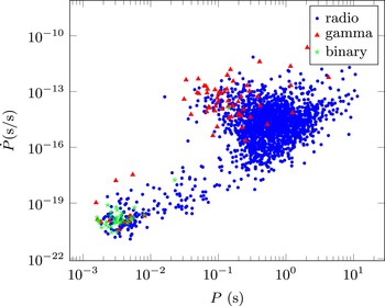
Figure 1.
 $P{-}{\dot{P}}$
diagram of all known pulsars with measured periods and period derivatives. Data are from the ATNF Pulsar Catalogue at http://www.atnf.csiro.au/people/
pulsar/psrcat/ and Manchester, R. N., Hobbs, G. B., Teoh, A. & Hobbs, M., AJ, 129, 1993–2006 (2005).
$P{-}{\dot{P}}$
diagram of all known pulsars with measured periods and period derivatives. Data are from the ATNF Pulsar Catalogue at http://www.atnf.csiro.au/people/
pulsar/psrcat/ and Manchester, R. N., Hobbs, G. B., Teoh, A. & Hobbs, M., AJ, 129, 1993–2006 (2005).
Although pulsars have been discovered through their radio emissions, this mechanism remains largely misunderstood. Moreover, only a fraction of
 $10^{-5}$
of the rotational kinetic luminosity is converted into radio power. The radio brightness temperature is of the order of
$10^{-5}$
of the rotational kinetic luminosity is converted into radio power. The radio brightness temperature is of the order of
 $T_{b}\approx 10^{25}{-}10^{28}$
K, and is thus not produced by a usual plasma process but via a coherent emission mechanism that still awaits elucidation. To obtain a more accurate idea of the pulsar machinery, it is compulsory to make a rigorous scrutiny of the physical conditions reigning inside its magnetosphere. The assumption of a rotating magnetic dipole loosing energy per vacuum electromagnetic radiation is unrealistic because we would only expected emission at the rotation frequency
$T_{b}\approx 10^{25}{-}10^{28}$
K, and is thus not produced by a usual plasma process but via a coherent emission mechanism that still awaits elucidation. To obtain a more accurate idea of the pulsar machinery, it is compulsory to make a rigorous scrutiny of the physical conditions reigning inside its magnetosphere. The assumption of a rotating magnetic dipole loosing energy per vacuum electromagnetic radiation is unrealistic because we would only expected emission at the rotation frequency
 $\unicode[STIX]{x1D6FA}$
, completely at odds with observations showing a broadband emission spectrum from MHz frequencies up to TeV energies. The rotational braking of the star, the nascent current in the magnetosphere circulating into the wind, the associated particle acceleration and transport of energy from the surface across the light cylinder up to the nebula therefore all require a detailed knowledge about pulsar electrodynamics, especially the longitudinal electric current (along magnetic field lines).
$\unicode[STIX]{x1D6FA}$
, completely at odds with observations showing a broadband emission spectrum from MHz frequencies up to TeV energies. The rotational braking of the star, the nascent current in the magnetosphere circulating into the wind, the associated particle acceleration and transport of energy from the surface across the light cylinder up to the nebula therefore all require a detailed knowledge about pulsar electrodynamics, especially the longitudinal electric current (along magnetic field lines).
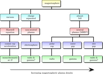
Figure 2. View of pulsar magnetosphere models depending on the plasma density in the magnetosphere. The upper cyan boxes indicate the three alternative magnetosphere assumptions. The red boxes describe the regime used to investigate the dynamics. The blue boxes point out the peculiarity of each model. The green boxes summarize the expected emission spectra.
For the sake of simplicity, we essentially distinguish three kind of magnetospheres, or more exactly three fundamental hypotheses of magnetosphere theory. At one extreme, we consider a naked star, entirely devoid of plasma in its immediate neighbourhood, the zeroth-order formulation, so to say. Of course, without plasma there is no high-energy emission but if the plasma density remains negligible, the dynamics only weakly depends on the plasma motion and properties. At the other extreme, we consider a star completely surrounded by a dense plasma, screening the longitudinal electric field
 $E_{\Vert }=\boldsymbol{E}\boldsymbol{\cdot }\boldsymbol{B}/B$
that would be imposed in vacuum by the previous assumption. In between these two conflicting starting points, an intermediate model admits the existence of a surrounding, partially filled or empty, magnetosphere, depending on our pessimistic or optimistic view, called an electrosphere. These three models and possible variations, as well as their related observational implications, are shown in figure 2. The place of the plasma density cursor is the discriminating parameter. The low density limit leads to nonlinear plasma wave models (Rajib, Sultana & Mamun Reference Rajib, Sultana and Mamun2015) whereas the high density limit was developed as a relativistic wind model. Pair production in the magnetosphere is the key process to determine which regime is to be applied and nothing forbids us from switching from one regime to another during plasma transport towards the nebula. Kennel, Fujimura & Pellat (Reference Kennel, Fujimura and Pellat1979) give orders of magnitude for the properties of these waves and winds. We briefly discuss the evolution of the ideas concerning pulsar magnetospheres which led to these three alternatives.
$E_{\Vert }=\boldsymbol{E}\boldsymbol{\cdot }\boldsymbol{B}/B$
that would be imposed in vacuum by the previous assumption. In between these two conflicting starting points, an intermediate model admits the existence of a surrounding, partially filled or empty, magnetosphere, depending on our pessimistic or optimistic view, called an electrosphere. These three models and possible variations, as well as their related observational implications, are shown in figure 2. The place of the plasma density cursor is the discriminating parameter. The low density limit leads to nonlinear plasma wave models (Rajib, Sultana & Mamun Reference Rajib, Sultana and Mamun2015) whereas the high density limit was developed as a relativistic wind model. Pair production in the magnetosphere is the key process to determine which regime is to be applied and nothing forbids us from switching from one regime to another during plasma transport towards the nebula. Kennel, Fujimura & Pellat (Reference Kennel, Fujimura and Pellat1979) give orders of magnitude for the properties of these waves and winds. We briefly discuss the evolution of the ideas concerning pulsar magnetospheres which led to these three alternatives.
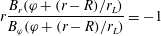
2.2 Vacuum electromagnetic fields
The simplest model we can think of relates to a vacuum magnetosphere, empty of any plasma or particles. To start with, the internal structure of a neutron star is believed to be in a superconducting and superfluid state. Its electric conductivity is so high that the magnetic field is frozen into the star and could survive for a long time. Moreover, because of its rotation, a electromotive field is induced such that the electric field in the corotating frame vanishes,
 $\boldsymbol{E}^{\prime }=0$
. Transformations of the electromagnetic field from one frame to another require general relativity (Kaburaki Reference Kaburaki1978) and not Lorentz transformations when rotation is considered. The question about electromagnetic fields in rotating frames was raised by Schiff (Reference Schiff1939) who discussed an illustrative example of two rotating and charged concentric spheres. Following his idea, Webster & Whitten (Reference Webster and Whitten1973) used the tensorial formalism of general relativity to write Maxwell equations in any rotating coordinate frame. Additional source terms in the inhomogeneous Maxwell equations appear in non-inertial frames. From the transformation law between an inertial frame and a rotating frame (Grøn Reference Grøn1984) we get
$\boldsymbol{E}^{\prime }=0$
. Transformations of the electromagnetic field from one frame to another require general relativity (Kaburaki Reference Kaburaki1978) and not Lorentz transformations when rotation is considered. The question about electromagnetic fields in rotating frames was raised by Schiff (Reference Schiff1939) who discussed an illustrative example of two rotating and charged concentric spheres. Following his idea, Webster & Whitten (Reference Webster and Whitten1973) used the tensorial formalism of general relativity to write Maxwell equations in any rotating coordinate frame. Additional source terms in the inhomogeneous Maxwell equations appear in non-inertial frames. From the transformation law between an inertial frame and a rotating frame (Grøn Reference Grøn1984) we get
 $$\begin{eqnarray}\displaystyle \boldsymbol{E}^{\prime }=\boldsymbol{E}+(\unicode[STIX]{x1D6FA}\wedge \boldsymbol{r})\wedge \boldsymbol{B}=0, & & \displaystyle\end{eqnarray}$$
where
 $\boldsymbol{r}$
is the position vector and
$\boldsymbol{r}$
is the position vector and
 $\unicode[STIX]{x1D734}$
the rotation velocity vector of the star. The interpretation of this relation was not that obvious (Backus Reference Backus1956). The usual picture of magnetic field line motion has been challenged by Newcomb (Reference Newcomb1958) and should be taken with care. From this equilibrium condition, we deduce that the electric and magnetic fields are perpendicular in any frame because of the Lorentz invariance of
$\unicode[STIX]{x1D734}$
the rotation velocity vector of the star. The interpretation of this relation was not that obvious (Backus Reference Backus1956). The usual picture of magnetic field line motion has been challenged by Newcomb (Reference Newcomb1958) and should be taken with care. From this equilibrium condition, we deduce that the electric and magnetic fields are perpendicular in any frame because of the Lorentz invariance of
 $\boldsymbol{E}\boldsymbol{\cdot }\boldsymbol{B}=0$
. In other words, magnetic field lines are equipotentials for the electric field. To solve completely the problem of this rotating conductor, we need an assumption about the internal magnetic field. Two simple choices often quoted are a uniform magnetic field inside the star or a point dipole located right at its centre. It is straightforward to show that, in both configurations, the external magnetic field is dipolar. For a rotator with an inclination between the rotation axis and either the magnetic moment or the direction of the uniform interior magnetic field depicted by an obliquity
$\boldsymbol{E}\boldsymbol{\cdot }\boldsymbol{B}=0$
. In other words, magnetic field lines are equipotentials for the electric field. To solve completely the problem of this rotating conductor, we need an assumption about the internal magnetic field. Two simple choices often quoted are a uniform magnetic field inside the star or a point dipole located right at its centre. It is straightforward to show that, in both configurations, the external magnetic field is dipolar. For a rotator with an inclination between the rotation axis and either the magnetic moment or the direction of the uniform interior magnetic field depicted by an obliquity
 $\unicode[STIX]{x1D712}$
, these expressions in spherical polar coordinates
$\unicode[STIX]{x1D712}$
, these expressions in spherical polar coordinates
 $(r,\unicode[STIX]{x1D717},\unicode[STIX]{x1D711})$
in the quasi-static near zone for distances much less than the wavelength
$(r,\unicode[STIX]{x1D717},\unicode[STIX]{x1D711})$
in the quasi-static near zone for distances much less than the wavelength
 $\unicode[STIX]{x1D706}=2\unicode[STIX]{x03C0}r_{L}$
where
$\unicode[STIX]{x1D706}=2\unicode[STIX]{x03C0}r_{L}$
where
 $r_{L}=c/\unicode[STIX]{x1D6FA}$
are given by
$r_{L}=c/\unicode[STIX]{x1D6FA}$
are given by
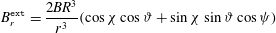 $$\begin{eqnarray}\displaystyle & \displaystyle B_{r}^{\text{ext}}=\frac{2BR^{3}}{r^{3}}(\cos \unicode[STIX]{x1D712}\cos \unicode[STIX]{x1D717}+\sin \unicode[STIX]{x1D712}\sin \unicode[STIX]{x1D717}\cos \unicode[STIX]{x1D713}) & \displaystyle\end{eqnarray}$$
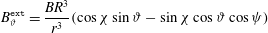 $$\begin{eqnarray}\displaystyle & \displaystyle B_{\unicode[STIX]{x1D717}}^{\text{ext}}=\frac{BR^{3}}{r^{3}}(\cos \unicode[STIX]{x1D712}\sin \unicode[STIX]{x1D717}-\sin \unicode[STIX]{x1D712}\cos \unicode[STIX]{x1D717}\cos \unicode[STIX]{x1D713}) & \displaystyle\end{eqnarray}$$
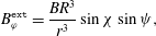 $$\begin{eqnarray}\displaystyle & \displaystyle B_{\unicode[STIX]{x1D711}}^{\text{ext}}=\frac{BR^{3}}{r^{3}}\sin \unicode[STIX]{x1D712}\sin \unicode[STIX]{x1D713}, & \displaystyle\end{eqnarray}$$
 $\unicode[STIX]{x1D713}=\unicode[STIX]{x1D711}-\unicode[STIX]{x1D6FA}t$
is the instantaneous phase at time
$\unicode[STIX]{x1D713}=\unicode[STIX]{x1D711}-\unicode[STIX]{x1D6FA}t$
is the instantaneous phase at time
 $t$
. The external electric field in vacuum is quadrupolar and its components read
$t$
. The external electric field in vacuum is quadrupolar and its components read  $$\begin{eqnarray}\displaystyle & \displaystyle E_{r}^{\text{ext}}=\unicode[STIX]{x1D6FA}BR\left[\frac{R^{4}}{r^{4}}\cos \unicode[STIX]{x1D712}(1-3\cos ^{2}\unicode[STIX]{x1D703})-3\frac{R^{4}}{r^{4}}\sin \unicode[STIX]{x1D712}\cos \unicode[STIX]{x1D703}\sin \unicode[STIX]{x1D703}\cos \unicode[STIX]{x1D713}\right]+\frac{Q_{\ast }}{4\unicode[STIX]{x03C0}\unicode[STIX]{x1D700}_{0}r^{2}} & \displaystyle \nonumber\\ \displaystyle & & \displaystyle\end{eqnarray}$$
 $$\begin{eqnarray}\displaystyle & \displaystyle E_{\unicode[STIX]{x1D703}}^{\text{ext}}=\unicode[STIX]{x1D6FA}BR\left[\frac{R^{2}}{r^{2}}\sin \unicode[STIX]{x1D712}\left(\frac{R^{2}}{r^{2}}\cos 2\unicode[STIX]{x1D703}-1\right)\cos \unicode[STIX]{x1D713}-\frac{R^{4}}{r^{4}}\cos \unicode[STIX]{x1D712}\sin 2\unicode[STIX]{x1D703}\right] & \displaystyle\end{eqnarray}$$
 $$\begin{eqnarray}\displaystyle & \displaystyle E_{\unicode[STIX]{x1D711}}^{\text{ext}}=\unicode[STIX]{x1D6FA}BR\frac{R^{2}}{r^{2}}\left(1-\frac{R^{2}}{r^{2}}\right)\sin \unicode[STIX]{x1D712}\cos \unicode[STIX]{x1D703}\sin \unicode[STIX]{x1D713}. & \displaystyle\end{eqnarray}$$
 $Q_{\ast }$
. Indeed, according to Gauss theorem, the asymptotic electric field has only a dominant radial component
$Q_{\ast }$
. Indeed, according to Gauss theorem, the asymptotic electric field has only a dominant radial component
 $E_{r}=Q_{\ast }/4\unicode[STIX]{x03C0}\unicode[STIX]{x1D700}_{0}r^{2}$
, that is a monopolar term.
$E_{r}=Q_{\ast }/4\unicode[STIX]{x03C0}\unicode[STIX]{x1D700}_{0}r^{2}$
, that is a monopolar term.
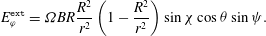
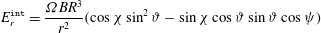
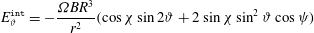
In order to deduce the electric field inside the star and to fully solve the electromagnetic problem in whole space, we need to distinguish between several magnetizations. Assuming a dipolar magnetic field inside, the electric field inside becomes
 $$\begin{eqnarray}\displaystyle & \displaystyle E_{r}^{\text{int}}=\frac{\unicode[STIX]{x1D6FA}BR^{3}}{r^{2}}(\cos \unicode[STIX]{x1D712}\sin ^{2}\unicode[STIX]{x1D717}-\sin \unicode[STIX]{x1D712}\cos \unicode[STIX]{x1D717}\sin \unicode[STIX]{x1D717}\cos \unicode[STIX]{x1D713}) & \displaystyle\end{eqnarray}$$
 $$\begin{eqnarray}\displaystyle & \displaystyle E_{\unicode[STIX]{x1D717}}^{\text{int}}=-\frac{\unicode[STIX]{x1D6FA}BR^{3}}{r^{2}}(\cos \unicode[STIX]{x1D712}\sin 2\unicode[STIX]{x1D717}+2\sin \unicode[STIX]{x1D712}\sin ^{2}\unicode[STIX]{x1D717}\cos \unicode[STIX]{x1D713}) & \displaystyle\end{eqnarray}$$
 $$\begin{eqnarray}\displaystyle & \displaystyle E_{\unicode[STIX]{x1D711}}^{\text{int}}=0. & \displaystyle\end{eqnarray}$$
 $$\begin{eqnarray}\displaystyle & \displaystyle B_{r}^{\text{int}}=2B(\cos \unicode[STIX]{x1D712}\cos \unicode[STIX]{x1D717}+\sin \unicode[STIX]{x1D712}\sin \unicode[STIX]{x1D717}\cos \unicode[STIX]{x1D713}) & \displaystyle\end{eqnarray}$$
 $$\begin{eqnarray}\displaystyle & \displaystyle B_{\unicode[STIX]{x1D717}}^{\text{int}}=2B(-\cos \unicode[STIX]{x1D712}\sin \unicode[STIX]{x1D717}+\sin \unicode[STIX]{x1D712}\cos \unicode[STIX]{x1D717}\cos \unicode[STIX]{x1D713}) & \displaystyle\end{eqnarray}$$
 $$\begin{eqnarray}\displaystyle & \displaystyle B_{\unicode[STIX]{x1D711}}^{\text{int}}=-2B\sin \unicode[STIX]{x1D712}\sin \unicode[STIX]{x1D713} & \displaystyle\end{eqnarray}$$
 $$\begin{eqnarray}\displaystyle & \displaystyle E_{r}^{\text{int}}=2r\unicode[STIX]{x1D6FA}B\sin \unicode[STIX]{x1D717}(-\cos \unicode[STIX]{x1D712}\sin \unicode[STIX]{x1D717}+\sin \unicode[STIX]{x1D712}\cos \unicode[STIX]{x1D717}\cos \unicode[STIX]{x1D713}) & \displaystyle\end{eqnarray}$$
 $$\begin{eqnarray}\displaystyle & \displaystyle E_{\unicode[STIX]{x1D717}}^{\text{int}}=-2r\unicode[STIX]{x1D6FA}B\sin \unicode[STIX]{x1D717}(\cos \unicode[STIX]{x1D712}\cos \unicode[STIX]{x1D717}+\sin \unicode[STIX]{x1D712}\sin \unicode[STIX]{x1D717}\cos \unicode[STIX]{x1D713}) & \displaystyle\end{eqnarray}$$
 $$\begin{eqnarray}\displaystyle & \displaystyle E_{\unicode[STIX]{x1D711}}^{\text{int}}=0. & \displaystyle\end{eqnarray}$$
 $r\ll \unicode[STIX]{x1D706}$
because they neglect the displacement current
$r\ll \unicode[STIX]{x1D706}$
because they neglect the displacement current
 $\unicode[STIX]{x1D700}_{0}\unicode[STIX]{x2202}_{t}\boldsymbol{E}$
. Let us have a look on the charge distribution inside the star and at its surface. In this approximation there is no surface current because of the quasi-static assumption. Discontinuities in the magnetic field responsible for this current include corrections of the order
$\unicode[STIX]{x1D700}_{0}\unicode[STIX]{x2202}_{t}\boldsymbol{E}$
. Let us have a look on the charge distribution inside the star and at its surface. In this approximation there is no surface current because of the quasi-static assumption. Discontinuities in the magnetic field responsible for this current include corrections of the order
 $O(\unicode[STIX]{x1D6FA})$
. From the perfect conductor condition (2.6) the density in the absence of electric current, which could be neglected because the advective and displacement terms are of the order
$O(\unicode[STIX]{x1D6FA})$
. From the perfect conductor condition (2.6) the density in the absence of electric current, which could be neglected because the advective and displacement terms are of the order
 $(r/r_{L})^{2}$
, is
$(r/r_{L})^{2}$
, is  $$\begin{eqnarray}\displaystyle \unicode[STIX]{x1D70C}_{e}=\unicode[STIX]{x1D700}_{0}\unicode[STIX]{x1D735}\boldsymbol{\cdot }\boldsymbol{E}=-2\unicode[STIX]{x1D700}_{0}\unicode[STIX]{x1D734}\boldsymbol{\cdot }\boldsymbol{B}. & & \displaystyle\end{eqnarray}$$
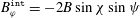
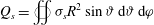
If the magnetization is dipolar, a central point charge exists, given by
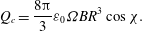 $$\begin{eqnarray}\displaystyle Q_{c}=\frac{8\unicode[STIX]{x03C0}}{3}\unicode[STIX]{x1D700}_{0}\unicode[STIX]{x1D6FA}BR^{3}\cos \unicode[STIX]{x1D712}. & & \displaystyle\end{eqnarray}$$
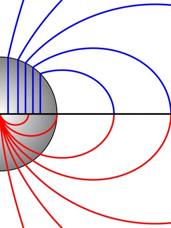
Figure 3. Uniform (upper blue) versus dipolar (lower red) internal magnetic field. Whatever the internal structure, outside the magnetic field is dipolar and the electric field quadrupolar to lowest order in
 $R/r_{L}$
.
$R/r_{L}$
.
Table 1. Properties of vacuum electrodynamics around neutron stars for a dipolar magnetization.
This charge should not be forgotten when computing the full electromagnetic field. The volume charge inside the star is zero between two spherical shells, the remaining distributes on its surface, inducing a discontinuity in the radial component of the electric field which is sustained by a surface electric charge
 $\unicode[STIX]{x1D70E}_{s}=\unicode[STIX]{x1D700}_{0}[E_{r}]$
. The central point charge is compensated by the stellar surface charge, as summarized in table 1. In the same vein, for a uniform magnetization, the constant volume charge density is compensated by the surface charge to keep the star electrically neutral whereas the central point charge has disappeared, see table 2. Tables 1 and 2 summarize the electric charge density inside the star and on its surface for both uniform and dipole magnetization and figure 3 shows the two magnetizations. For completeness, the total volume and surface charges are also computed according to
$\unicode[STIX]{x1D70E}_{s}=\unicode[STIX]{x1D700}_{0}[E_{r}]$
. The central point charge is compensated by the stellar surface charge, as summarized in table 1. In the same vein, for a uniform magnetization, the constant volume charge density is compensated by the surface charge to keep the star electrically neutral whereas the central point charge has disappeared, see table 2. Tables 1 and 2 summarize the electric charge density inside the star and on its surface for both uniform and dipole magnetization and figure 3 shows the two magnetizations. For completeness, the total volume and surface charges are also computed according to
 $$\begin{eqnarray}\displaystyle & \displaystyle Q_{v}=\iiint \unicode[STIX]{x1D70C}_{e}r^{2}\sin \unicode[STIX]{x1D717}\,\text{d}r\,\text{d}\unicode[STIX]{x1D717}\,\text{d}\unicode[STIX]{x1D711} & \displaystyle\end{eqnarray}$$
 $$\begin{eqnarray}\displaystyle & \displaystyle Q_{s}=\unicode[STIX]{x0222F}\unicode[STIX]{x1D70E}_{s}R^{2}\sin \unicode[STIX]{x1D717}\,\text{d}\unicode[STIX]{x1D717}\,\text{d}\unicode[STIX]{x1D711} & \displaystyle\end{eqnarray}$$
 $Q_{\ast }=Q_{v}+Q_{s}$
. The neutron star even if surrounded by vacuum could have an atmosphere because of its high surface temperature of
$Q_{\ast }=Q_{v}+Q_{s}$
. The neutron star even if surrounded by vacuum could have an atmosphere because of its high surface temperature of
 $T\approx 10^{6}$
K. However the thickness of this layer would be very tiny because the height scale for a totally ionized hydrogen gas is
$T\approx 10^{6}$
K. However the thickness of this layer would be very tiny because the height scale for a totally ionized hydrogen gas is  $$\begin{eqnarray}\displaystyle H=\frac{k_{B}T}{GMm_{H}/R^{2}}\approx 4.4~\text{m}\text{m}\times \left(\frac{M}{1.4~M_{\odot }}\right)\left(\frac{T}{10^{6}~\text{K}}\right)^{-1}\left(\frac{R}{10^{4}~\text{m}}\right)^{2}. & & \displaystyle\end{eqnarray}$$
At electrostatic equilibrium, the electromotive field displaces charges, initially interior to the pulsar, to its surface where they accumulate to screen this field. Other charges redistribute in such a way that in the rest frame of the star the total electric field vanishes. At the stellar surface an electric field appears of the order
 $$\begin{eqnarray}\displaystyle E=\unicode[STIX]{x1D6FA}BR=10^{13}~\text{V}~\text{m}^{-1}. & & \displaystyle\end{eqnarray}$$
This huge field extracts charges from the surface despite the presence of a potential barrier imposed by the inter- and intra-molecular attractionFootnote
2
. This extraction threshold can be neglected without difficulty for a pulsar (at least for the electrons and probably also for the ions). The distinction between particle extraction and no particle extraction leads to different pulsar atmospheric models, a possible explanation for the evolution of pulsar states (Endean Reference Endean1973). The vacuum model could also apply to low density plasmas. By low density Endean & Allen (Reference Endean and Allen1970) meant
 $n<19$
particles m
$n<19$
particles m
 $^{-3}$
for instance for the Crab. They proposed a model where particle corotation is only reached at twice the light-cylinder radius,
$^{-3}$
for instance for the Crab. They proposed a model where particle corotation is only reached at twice the light-cylinder radius,
 $r=2r_{L}$
. When crossing this surface, particles become highly relativistic and radiate synchrotron photons in regions forming a two-armed spiral where
$r=2r_{L}$
. When crossing this surface, particles become highly relativistic and radiate synchrotron photons in regions forming a two-armed spiral where
 $E_{\bot }>cB$
.
$E_{\bot }>cB$
.
Table 2. Properties of vacuum electrodynamics around neutron stars for a uniform magnetization.
2.3 Some historical notes
The exact analytical solution to the external problem, taking into account the boundary condition on the neutron star surface and the displacement current, is given by the Deutsch (Reference Deutsch1955) solution whether the magnetization is dipolar or uniform. Indeed, as shown in Pétri (Reference Pétri2015d
), the electromagnetic field in vacuum outside the star is entirely determined by the radial component of the magnetic field at the surface,
 $B_{r}$
. As this component is the same for both magnetizations, we expect the same solution outside the star. The only difference reflects in the surface charge and current densities, thus accounting for different spin-down luminosities and torques exerted on the star.
$B_{r}$
. As this component is the same for both magnetizations, we expect the same solution outside the star. The only difference reflects in the surface charge and current densities, thus accounting for different spin-down luminosities and torques exerted on the star.
Deutsch (Reference Deutsch1955) was the first to compute the electromagnetic wave emission emanating from a magnetized star in solid body rotation. He found that for those stars with a strong magnetic field and fast rotation, the induced electric field becomes so strong that it is able to accelerate particles of the circumstellar medium to relativistic, and even ultra-relativistic, speeds. He thought that this phenomenon was the source for cosmic rays, an idea which is still valid. The rotating magnetized star is therefore at the origin of charge acceleration. At that time, he did not mention neutron stars. Moreover, his computations were valid only for a star plunged in vacuum. The star only emits a monochromatic large-amplitude electromagnetic wave at a frequency equal to the stellar rotation rate
 $\unicode[STIX]{x1D6FA}$
. The exact analytical solution he found is
$\unicode[STIX]{x1D6FA}$
. The exact analytical solution he found is
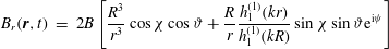 $$\begin{eqnarray}\displaystyle B_{r}(\boldsymbol{r},t) & = & \displaystyle 2B\left[\frac{R^{3}}{r^{3}}\cos \unicode[STIX]{x1D712}\cos \unicode[STIX]{x1D717}+\frac{R}{r}\frac{h_{1}^{(1)}(kr)}{h_{1}^{(1)}(kR)}\sin \unicode[STIX]{x1D712}\sin \unicode[STIX]{x1D717}\text{e}^{\text{i}\unicode[STIX]{x1D713}}\right]\end{eqnarray}$$
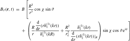 $$\begin{eqnarray}\displaystyle B_{\unicode[STIX]{x1D717}}(\boldsymbol{r},t) & = & \displaystyle B\left[\frac{R^{3}}{r^{3}}\cos \unicode[STIX]{x1D712}\sin \unicode[STIX]{x1D717}\right.\nonumber\\ \displaystyle & & \displaystyle +\,\left.\left(\frac{R}{r}\frac{\displaystyle \frac{\text{d}}{\text{d}r}(rh_{1}^{(1)}(kr))}{h_{1}^{(1)}(kR)}+\frac{R^{2}}{r_{L}^{2}}\frac{h_{2}^{(1)}(kr)}{\displaystyle \frac{\text{d}}{\text{d}r}(rh_{2}^{(1)}(kr))|_{R}}\right)\sin \unicode[STIX]{x1D712}\cos \unicode[STIX]{x1D717}\text{e}^{\text{i}\unicode[STIX]{x1D713}}\right]\end{eqnarray}$$
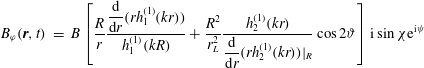 $$\begin{eqnarray}\displaystyle B_{\unicode[STIX]{x1D711}}(\boldsymbol{r},t) & = & \displaystyle B\left[\frac{R}{r}\frac{\displaystyle \frac{\text{d}}{\text{d}r}(rh_{1}^{(1)}(kr))}{h_{1}^{(1)}(kR)}+\frac{R^{2}}{r_{L}^{2}}\frac{h_{2}^{(1)}(kr)}{\displaystyle \frac{\text{d}}{\text{d}r}(rh_{2}^{(1)}(kr))|_{R}}\cos 2\unicode[STIX]{x1D717}\right]\text{i}\sin \unicode[STIX]{x1D712}\text{e}^{\text{i}\unicode[STIX]{x1D713}}\end{eqnarray}$$
 $k=1/r_{L}$
is the wavenumber and
$k=1/r_{L}$
is the wavenumber and
 $h_{\ell }^{(1)}$
are the spherical Hankel functions of order
$h_{\ell }^{(1)}$
are the spherical Hankel functions of order
 $\ell$
satisfying the outgoing wave conditions, see for instance Arfken & Weber (Reference Arfken and Weber2005). The induced electric field is then
$\ell$
satisfying the outgoing wave conditions, see for instance Arfken & Weber (Reference Arfken and Weber2005). The induced electric field is then
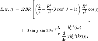 $$\begin{eqnarray}\displaystyle E_{r}(\boldsymbol{r},t) & = & \displaystyle \unicode[STIX]{x1D6FA}BR\left[\left(\frac{2}{3}-\frac{R^{2}}{r^{2}}(3\cos ^{2}\unicode[STIX]{x1D717}-1)\right)\frac{R^{2}}{r^{2}}\cos \unicode[STIX]{x1D712}\right.\nonumber\\ \displaystyle & & \displaystyle +\,\left.3\sin \unicode[STIX]{x1D712}\sin 2\unicode[STIX]{x1D717}\text{e}^{\text{i}\unicode[STIX]{x1D713}}\frac{R}{r}\frac{h_{2}^{(1)}(kr)}{\displaystyle \frac{\text{d}}{\text{d}r}(rh_{2}^{(1)}(kr))|_{R}}\right]\end{eqnarray}$$
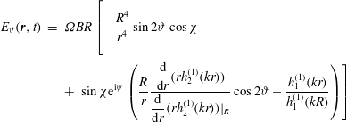 $$\begin{eqnarray}\displaystyle E_{\unicode[STIX]{x1D717}}(\boldsymbol{r},t) & = & \displaystyle \unicode[STIX]{x1D6FA}BR\left[-\frac{R^{4}}{r^{4}}\sin 2\unicode[STIX]{x1D717}\cos \unicode[STIX]{x1D712}\right.\nonumber\\ \displaystyle & & \displaystyle +\,\left.\sin \unicode[STIX]{x1D712}\text{e}^{\text{i}\unicode[STIX]{x1D713}}\left(\frac{R}{r}\frac{\displaystyle \frac{\text{d}}{\text{d}r}(rh_{2}^{(1)}(kr))}{\displaystyle \frac{\text{d}}{\text{d}r}(rh_{2}^{(1)}(kr))|_{R}}\cos 2\unicode[STIX]{x1D717}-\frac{h_{1}^{(1)}(kr)}{h_{1}^{(1)}(kR)}\right)\right]\end{eqnarray}$$
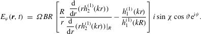 $$\begin{eqnarray}\displaystyle E_{\unicode[STIX]{x1D711}}(\boldsymbol{r},t) & = & \displaystyle \unicode[STIX]{x1D6FA}BR\left[\frac{R}{r}\frac{\displaystyle \frac{\text{d}}{\text{d}r}(rh_{2}^{(1)}(kr))}{\displaystyle \frac{\text{d}}{\text{d}r}(rh_{2}^{(1)}(kr))|_{R}}-\frac{h_{1}^{(1)}(kr)}{h_{1}^{(1)}(kR)}\right]i\sin \unicode[STIX]{x1D712}\cos \unicode[STIX]{x1D717}\text{e}^{\text{i}\unicode[STIX]{x1D713}}.\end{eqnarray}$$
The physical solution is found by taking the real parts of each component. It encompasses a linear combination of the vacuum aligned dipole field and the vacuum orthogonal rotator with respective weights
 $\cos \unicode[STIX]{x1D712}$
and
$\cos \unicode[STIX]{x1D712}$
and
 $\sin \unicode[STIX]{x1D712}$
. To complete the solution for arbitrary stellar electrical charge, we add a monopolar electric field contribution due to the stellar surface charge such that
$\sin \unicode[STIX]{x1D712}$
. To complete the solution for arbitrary stellar electrical charge, we add a monopolar electric field contribution due to the stellar surface charge such that
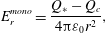 $$\begin{eqnarray}\displaystyle E_{r}^{mono}=\frac{Q_{\ast }-Q_{c}}{4\unicode[STIX]{x03C0}\unicode[STIX]{x1D700}_{0}r^{2}}, & & \displaystyle\end{eqnarray}$$

Figure 4. Magnetic field lines (red solid lines) of the Deutsch solution for the orthogonal rotator with
 $R/r_{L}=0.2$
. The right panel is a zoom-in on central region close to the light cylinder (the dashed black circle of radius unity). The two-armed blue spiral line depicts the large-scale wave structure of the electromagnetic field.
$R/r_{L}=0.2$
. The right panel is a zoom-in on central region close to the light cylinder (the dashed black circle of radius unity). The two-armed blue spiral line depicts the large-scale wave structure of the electromagnetic field.
where
 $Q_{\ast }$
is the total electric charge of the star. This term compensates the
$Q_{\ast }$
is the total electric charge of the star. This term compensates the
 $\cos \unicode[STIX]{x1D712}/r^{2}$
decrease of
$\cos \unicode[STIX]{x1D712}/r^{2}$
decrease of
 $E_{r}$
in (2.16d
). The Deutsch solution separates space around a magnet into three distinct regions: the near or quasi-static zone where
$E_{r}$
in (2.16d
). The Deutsch solution separates space around a magnet into three distinct regions: the near or quasi-static zone where
 $r\ll r_{L}$
and for which the above expressions reduce to the static oblique dipole (2.7)–(2.8), the transition zone
$r\ll r_{L}$
and for which the above expressions reduce to the static oblique dipole (2.7)–(2.8), the transition zone
 $r\approx r_{L}$
and the wave zone
$r\approx r_{L}$
and the wave zone
 $r\gg r_{L}$
where the electromagnetic field resembles a transverse electromagnetic plane wave with an elliptical polarization, circular polarization along the rotation axis and linear polarization along the equatorial plane. An example of magnetic field lines in the equatorial plane is shown for the orthogonal rotator as red solid lines in figure 4. The radial component of
$r\gg r_{L}$
where the electromagnetic field resembles a transverse electromagnetic plane wave with an elliptical polarization, circular polarization along the rotation axis and linear polarization along the equatorial plane. An example of magnetic field lines in the equatorial plane is shown for the orthogonal rotator as red solid lines in figure 4. The radial component of
 $(\boldsymbol{B},\boldsymbol{E})$
decreases like
$(\boldsymbol{B},\boldsymbol{E})$
decreases like
 $1/r^{2}$
whereas the transverse component of
$1/r^{2}$
whereas the transverse component of
 $(\boldsymbol{B},\boldsymbol{E})$
decreases like
$(\boldsymbol{B},\boldsymbol{E})$
decreases like
 $1/r$
, typical for radiating fields in three-dimensional space. To better catch the geometry of the field lines, let us focus on the perpendicular rotating dipole with
$1/r$
, typical for radiating fields in three-dimensional space. To better catch the geometry of the field lines, let us focus on the perpendicular rotating dipole with
 $\unicode[STIX]{x1D712}=\unicode[STIX]{x03C0}/2$
. In the asymptotic limit when
$\unicode[STIX]{x1D712}=\unicode[STIX]{x03C0}/2$
. In the asymptotic limit when
 $r\rightarrow +\infty$
, in the equatorial plane we find a constant ratio
$r\rightarrow +\infty$
, in the equatorial plane we find a constant ratio
 $$\begin{eqnarray}\displaystyle r\frac{B_{r}}{B_{\unicode[STIX]{x1D711}}}=\text{cst}. & & \displaystyle\end{eqnarray}$$
As explained by Michel & Li (Reference Michel and Li1999) there are only two open field lines asymptoting to these Archimedean spirals. Their exact expressions at a fixed time are given in implicit form by
 $$\begin{eqnarray}\displaystyle r\frac{B_{r}(\unicode[STIX]{x1D711}+(r-R)/r_{L})}{B_{\unicode[STIX]{x1D711}}(\unicode[STIX]{x1D711}+(r-R)/r_{L})}=-1 & & \displaystyle\end{eqnarray}$$
to be solved for
 $\unicode[STIX]{x1D711}$
with respect to
$\unicode[STIX]{x1D711}$
with respect to
 $r$
. The two solutions are shown as blue solid lines in figure 4 as a two-armed spiral. Asymptotically, this spiral coincides with the
$r$
. The two solutions are shown as blue solid lines in figure 4 as a two-armed spiral. Asymptotically, this spiral coincides with the
 $B_{r}=0$
loci (Kaburaki Reference Kaburaki1980). Kaburaki (Reference Kaburaki1978) gave approximate analytical solutions in the near and wave zones for a uniformly magnetized rotating dipole using a scalar and vector potential description instead of electric and magnetic fields. Subsequently, Kaburaki (Reference Kaburaki1980) improved the method and gave exact analytical expressions by using rigid rotation, retardation and radiation operators applied to the static dipole. Then Kaburaki (Reference Kaburaki1981) solved the so-called modified Deutsch problem, that is, taking into account corotating plasma up to at most the light cylinder without poloidal current but approximately including inertial effects which were fully treated by Kaburaki (Reference Kaburaki1982). A self-consistent description then required the presence of a disk in the corotation zone (Kaburaki Reference Kaburaki1983). The Deutsch vacuum solution can also be expressed in the corotating frame (Ferrari & Trussoni Reference Ferrari and Trussoni1973).
$B_{r}=0$
loci (Kaburaki Reference Kaburaki1980). Kaburaki (Reference Kaburaki1978) gave approximate analytical solutions in the near and wave zones for a uniformly magnetized rotating dipole using a scalar and vector potential description instead of electric and magnetic fields. Subsequently, Kaburaki (Reference Kaburaki1980) improved the method and gave exact analytical expressions by using rigid rotation, retardation and radiation operators applied to the static dipole. Then Kaburaki (Reference Kaburaki1981) solved the so-called modified Deutsch problem, that is, taking into account corotating plasma up to at most the light cylinder without poloidal current but approximately including inertial effects which were fully treated by Kaburaki (Reference Kaburaki1982). A self-consistent description then required the presence of a disk in the corotation zone (Kaburaki Reference Kaburaki1983). The Deutsch vacuum solution can also be expressed in the corotating frame (Ferrari & Trussoni Reference Ferrari and Trussoni1973).
However, the presence of plasma modifies that picture because charge acceleration in the magnetosphere leads to an electromagnetic activity detectable on Earth. This activity induces a multi-wavelength emission spectrum as suggested by Gold (Reference Gold1968) for neutron stars. The possible association between the Vela supernova remnant and its central pulsar was already discussed by Large, Vaughan & Mills (Reference Large, Vaughan and Mills1968). The first model for an electromagnetically active neutron star was proposed by Pacini (Reference Pacini1967). Then Pacini (Reference Pacini1968) claimed that a rotating neutron star was the source of energy feeding the Crab nebula with fresh particles and admitted that a strong magnetic field transmits rotational kinetic energy from the star to the nebula via production of high-energy particles. From the work of Deutsch (Reference Deutsch1955) he deduced the energy radiated by such a star and concluded that a strongly magnetized neutron star located at the centre of the Crab nebula was responsible for the luminosity of its nebula, which was in agreement with observations. This idea was proposed even before the discovery of the first pulsar! He envisaged the existence of a star possessing a purely dipolar magnetic field, its magnetic moment
 $\unicode[STIX]{x1D741}$
making an angle
$\unicode[STIX]{x1D741}$
making an angle
 $\unicode[STIX]{x1D712}$
with respect to the rotation axis. Rotation of the magnetic dipole dragged by the star induces emission of a monochromatic electromagnetic wave at the star frequency
$\unicode[STIX]{x1D712}$
with respect to the rotation axis. Rotation of the magnetic dipole dragged by the star induces emission of a monochromatic electromagnetic wave at the star frequency
 $\unicode[STIX]{x1D6FA}$
. The radiation has a dipolar pattern and its total intensity is given by
$\unicode[STIX]{x1D6FA}$
. The radiation has a dipolar pattern and its total intensity is given by
 $L=L_{\bot }^{vac}\sin ^{2}\unicode[STIX]{x1D712}$
where the luminosity of a perpendicular rotator is
$L=L_{\bot }^{vac}\sin ^{2}\unicode[STIX]{x1D712}$
where the luminosity of a perpendicular rotator is
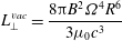 $$\begin{eqnarray}\displaystyle L_{\bot }^{vac}=\frac{8\unicode[STIX]{x03C0}B^{2}\unicode[STIX]{x1D6FA}^{4}R^{6}}{3\unicode[STIX]{x1D707}_{0}c^{3}} & & \displaystyle\end{eqnarray}$$
 $B$
is the magnetic field at the equator and
$B$
is the magnetic field at the equator and
 $R$
the neutron star radius. A more general prescription for the spin down luminosity, valid in the presence of a plasma, would be to set
$R$
the neutron star radius. A more general prescription for the spin down luminosity, valid in the presence of a plasma, would be to set
 $L=f(\unicode[STIX]{x1D712})L_{\bot }^{vac}$
. The function
$L=f(\unicode[STIX]{x1D712})L_{\bot }^{vac}$
. The function
 $f$
hides the precise microphysics inside the magnetosphere. We will come back to this point when discussing numerical simulations able to determine
$f$
hides the precise microphysics inside the magnetosphere. We will come back to this point when discussing numerical simulations able to determine
 $f$
depending on the plasma regime. In any case, this energy is not extracted from nuclear reactions nor from the collapse of the star. It is drained from the rotational kinetic energy reservoir containing a huge amount of energy, estimated to be
$f$
depending on the plasma regime. In any case, this energy is not extracted from nuclear reactions nor from the collapse of the star. It is drained from the rotational kinetic energy reservoir containing a huge amount of energy, estimated to be
 $$\begin{eqnarray}\displaystyle E_{rot}=\frac{1}{2}I\unicode[STIX]{x1D6FA}^{2}=2\unicode[STIX]{x03C0}^{2}IP^{-2}\approx 1.97\cdot 10^{39}~\text{J}\left(\frac{I}{10^{38}~\text{kg}\text{m}^{2}}\right)\left(\frac{P}{1~\text{s}}\right)^{-2}, & & \displaystyle\end{eqnarray}$$
with
 $I$
the stellar moment of inertia, equal to
$I$
the stellar moment of inertia, equal to
 $(2/5)MR^{2}$
for a homogeneous sphere. The power radiated exhausts this energy
$(2/5)MR^{2}$
for a homogeneous sphere. The power radiated exhausts this energy
 $E_{kin}$
and generates a luminosity following the relation
$E_{kin}$
and generates a luminosity following the relation
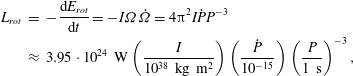 $$\begin{eqnarray}\displaystyle L_{rot} & = & \displaystyle -\frac{\text{d}E_{rot}}{\text{d}t}=-I\unicode[STIX]{x1D6FA}\dot{\unicode[STIX]{x1D6FA}}=4\unicode[STIX]{x03C0}^{2}I{\dot{P}}P^{-3}\nonumber\\ \displaystyle & {\approx} & \displaystyle 3.95\cdot 10^{24}~\text{W}\left(\frac{I}{10^{38}~\text{kg}~\text{m}^{2}}\right)\left(\frac{{\dot{P}}}{10^{-15}}\right)\left(\frac{P}{1~\text{s}}\right)^{-3},\end{eqnarray}$$
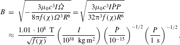
with a typical spin-down time scale of
 $\unicode[STIX]{x1D70F}=P/2{\dot{P}}$
known as the characteristic age of the pulsar. A piece of useful information about the brake efficiency is depicted by the braking index defined by
$\unicode[STIX]{x1D70F}=P/2{\dot{P}}$
known as the characteristic age of the pulsar. A piece of useful information about the brake efficiency is depicted by the braking index defined by
 $$\begin{eqnarray}\displaystyle n=\frac{\unicode[STIX]{x1D6FA}\ddot{\unicode[STIX]{x1D6FA}}}{\dot{\unicode[STIX]{x1D6FA}}^{2}}. & & \displaystyle\end{eqnarray}$$
Without any a priori knowledge of the secular evolution of all pulsar parameters such as magnetic field
 $B$
, electric equivalent radius
$B$
, electric equivalent radius
 $R_{el}$
, moment of inertia
$R_{el}$
, moment of inertia
 $I$
and inclination angle
$I$
and inclination angle
 $\unicode[STIX]{x1D712}$
, the braking index according to vacuum magnetodipole losses is
$\unicode[STIX]{x1D712}$
, the braking index according to vacuum magnetodipole losses is
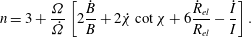 $$\begin{eqnarray}\displaystyle n=3+\frac{\unicode[STIX]{x1D6FA}}{\dot{\unicode[STIX]{x1D6FA}}}\left[2\frac{{\dot{B}}}{B}+2\dot{\unicode[STIX]{x1D712}}\cot \unicode[STIX]{x1D712}+6\frac{{\dot{R}}_{el}}{R_{el}}-\frac{{\dot{I}}}{I}\right]. & & \displaystyle\end{eqnarray}$$
The electric equivalent radius
 $R_{el}$
is a fictive boundary of the star which accounts for the replenishing of the corotating magnetosphere with plasma that, from an electrical point of view, is indistinguishable from the star. Such a concept of radius was introduced by Melatos (Reference Melatos1997) to account for spin-down properties of the Crab pulsar.
$R_{el}$
is a fictive boundary of the star which accounts for the replenishing of the corotating magnetosphere with plasma that, from an electrical point of view, is indistinguishable from the star. Such a concept of radius was introduced by Melatos (Reference Melatos1997) to account for spin-down properties of the Crab pulsar.
Energy losses are accompanied by a torque exerted on the neutron star that brakes its rotation according to (2.22), thus applying a torque along the rotation axis
 $\boldsymbol{e}_{z}$
but also a torque in the perpendicular plane tending to align the magnetic moment with the rotation axis: the anomalous torque. In the vacuum solution, this happens following the integral of motion
$\boldsymbol{e}_{z}$
but also a torque in the perpendicular plane tending to align the magnetic moment with the rotation axis: the anomalous torque. In the vacuum solution, this happens following the integral of motion
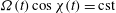 $\unicode[STIX]{x1D6FA}(t)\cos \unicode[STIX]{x1D712}(t)=\text{cst}$
(Davis & Goldstein Reference Davis and Goldstein1970; Michel & Goldwire Reference Michel and Goldwire1970) deduced from the spin-down torque
$\unicode[STIX]{x1D6FA}(t)\cos \unicode[STIX]{x1D712}(t)=\text{cst}$
(Davis & Goldstein Reference Davis and Goldstein1970; Michel & Goldwire Reference Michel and Goldwire1970) deduced from the spin-down torque
 $\dot{\unicode[STIX]{x1D6FA}}\propto \unicode[STIX]{x1D6FA}^{3}\sin ^{2}\unicode[STIX]{x1D712}$
and therefore a braking index (keeping other parameters constant in time) evolving in time according to
$\dot{\unicode[STIX]{x1D6FA}}\propto \unicode[STIX]{x1D6FA}^{3}\sin ^{2}\unicode[STIX]{x1D712}$
and therefore a braking index (keeping other parameters constant in time) evolving in time according to
 $$\begin{eqnarray}\displaystyle n=3+2\cot ^{2}\unicode[STIX]{x1D712}(t). & & \displaystyle\end{eqnarray}$$
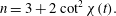
For a filled magnetosphere, loss by a charged wind from the poles induces an increase of obliquity with a decrease of rotation rate because of the integral of motion
 $\unicode[STIX]{x1D6FA}(t)\sin \unicode[STIX]{x1D712}(t)=\text{cst}$
, see Beskin et al. (Reference Beskin, Chernov, Gwinn and Tchekhovskoy2015). Assuming a spin-down like
$\unicode[STIX]{x1D6FA}(t)\sin \unicode[STIX]{x1D712}(t)=\text{cst}$
, see Beskin et al. (Reference Beskin, Chernov, Gwinn and Tchekhovskoy2015). Assuming a spin-down like
 $\dot{\unicode[STIX]{x1D6FA}}\propto \unicode[STIX]{x1D6FA}^{3}\cos ^{2}\unicode[STIX]{x1D712}$
the braking index now becomes
$\dot{\unicode[STIX]{x1D6FA}}\propto \unicode[STIX]{x1D6FA}^{3}\cos ^{2}\unicode[STIX]{x1D712}$
the braking index now becomes
 $$\begin{eqnarray}\displaystyle n=3+2\tan ^{2}\unicode[STIX]{x1D712}(t), & & \displaystyle\end{eqnarray}$$
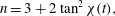
which also stays above
 $n=3$
, conflicting with measurements of braking index for eight pulsars summarized in Hamil et al. (Reference Hamil, Stone, Urbanec and Urbancová2015). However, the spin-down torque obtained by Beskin et al. (Reference Beskin, Chernov, Gwinn and Tchekhovskoy2015) seems to be based on an unphysical solution. Another expression, more involved, found by Beskin, Gurevich & Istomin (Reference Beskin, Gurevich and Istomin1993) is
$n=3$
, conflicting with measurements of braking index for eight pulsars summarized in Hamil et al. (Reference Hamil, Stone, Urbanec and Urbancová2015). However, the spin-down torque obtained by Beskin et al. (Reference Beskin, Chernov, Gwinn and Tchekhovskoy2015) seems to be based on an unphysical solution. Another expression, more involved, found by Beskin, Gurevich & Istomin (Reference Beskin, Gurevich and Istomin1993) is
 $$\begin{eqnarray}\displaystyle n=1.93+1.5\tan ^{2}\unicode[STIX]{x1D712}(t) & & \displaystyle\end{eqnarray}$$
thus able to yield braking indices much less than 3. Michel (Reference Michel1987) demonstrated that the torque in realistic magnetospheres is always aligning because, independently of any details, open magnetic field lines always bent backward with respect to rotation. Moreover, as already pointed out by Soper (Reference Soper1972), the vacuum results should not straightforwardly transpose to the more realistic plasma filled magnetosphere. Indeed, the plasma filled magnetosphere evolution of the inclination angle offers another interpretation of a braking index larger than 3 (Ekşi et al. Reference Ekşi, Andaç, Çıkıntoğlu, Gügercinoğlu, Vahdat Motlagh and Kızıltan2016). In the same vain, Philippov, Tchekhovskoy & Li (Reference Philippov, Tchekhovskoy and Li2014) accounted for plasma filled magnetospheres in the force-free and MHD limit contributing to the total torque and therefore to the subsequent obliquity evolution.
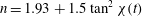
Applied to the Crab nebula, formula (2.22) indicates that the pulsar furnishes a power of the order
 $10^{31}$
W, a value remarkably close to what the surrounding nebula radiates. Thus, it is the rotational braking of the pulsar that feeds the nebula with particles and energy. Such a braking needs a gigantic magnetic field, estimated by equating the power lost by the neutron star (2.22) with the magnetodipole emission of an oblique rotator (2.20) to obtain
$10^{31}$
W, a value remarkably close to what the surrounding nebula radiates. Thus, it is the rotational braking of the pulsar that feeds the nebula with particles and energy. Such a braking needs a gigantic magnetic field, estimated by equating the power lost by the neutron star (2.22) with the magnetodipole emission of an oblique rotator (2.20) to obtain
 $$\begin{eqnarray}\displaystyle B & = & \displaystyle \sqrt{-\frac{3\unicode[STIX]{x1D707}_{0}c^{3}I\dot{\unicode[STIX]{x1D6FA}}}{8\unicode[STIX]{x03C0}f(\unicode[STIX]{x1D712})\unicode[STIX]{x1D6FA}^{3}R^{6}}}=\sqrt{\frac{3\unicode[STIX]{x1D707}_{0}c^{3}I{\dot{P}}P}{32\unicode[STIX]{x03C0}^{3}f(\unicode[STIX]{x1D712})R^{6}}}\nonumber\\ \displaystyle & {\approx} & \displaystyle \frac{1.01\cdot 10^{8}~\text{T}}{\sqrt{f(\unicode[STIX]{x1D712})}}\left(\frac{I}{10^{38}~\text{kg}\,\text{m}^{2}}\right)\left(\frac{{\dot{P}}}{10^{-15}}\right)^{-1/2}\left(\frac{P}{1~\text{s}}\right)^{-1/2}.\end{eqnarray}$$
For the Crab this gives approximately
 $10^{8}$
T. Ostriker & Gunn (Reference Ostriker and Gunn1969) were the first to envisage such magnetic field strengths. Gunn & Ostriker (Reference Gunn and Ostriker1969) have also investigated the acceleration of particles to very high energy pushed by such large-amplitude low-frequency electromagnetic waves. This intensity of the field was confirmed by the synchrotron spectra of the pulsar. However, this model does not explain the origin of the pulsed radio emission because it does not describe how to produce and accelerate particles, the magnetosphere being empty. Noticing that radiation needs particle acceleration, it became quickly clear that the magnetosphere could not remain empty. Several scenarios have therefore been proposed. Gold (Reference Gold1968) explained radio emission by a conglomerate of electrons in corotation with the star. This idea of formation of a bunch of electrons responsible for the coherent emission has then been invoked many times in recent models.
$10^{8}$
T. Ostriker & Gunn (Reference Ostriker and Gunn1969) were the first to envisage such magnetic field strengths. Gunn & Ostriker (Reference Gunn and Ostriker1969) have also investigated the acceleration of particles to very high energy pushed by such large-amplitude low-frequency electromagnetic waves. This intensity of the field was confirmed by the synchrotron spectra of the pulsar. However, this model does not explain the origin of the pulsed radio emission because it does not describe how to produce and accelerate particles, the magnetosphere being empty. Noticing that radiation needs particle acceleration, it became quickly clear that the magnetosphere could not remain empty. Several scenarios have therefore been proposed. Gold (Reference Gold1968) explained radio emission by a conglomerate of electrons in corotation with the star. This idea of formation of a bunch of electrons responsible for the coherent emission has then been invoked many times in recent models.
Goldreich & Julian (Reference Goldreich and Julian1969) examined in detail the aligned rotator. They noticed that an empty magnetosphere cannot last for a reasonable time because of strong electric fields induced by rotation of the magnetic moment, pulling particles out from the surface and dragging them in corotation with the star up to the light cylinder. Farther away a wind is formed, made of charged particles. The polar caps represent therefore a first choice region to explain radio emission. It is strictly speaking not a model for real pulsars because no pulsation is predicted for an aligned configuration assuming axisymmetry. However, Goldreich (Reference Goldreich1969) stipulated that the physics of an oblique rotator should not be very different from that of an aligned rotator. The very popular hollow cone model was born (Radhakrishnan & Cooke Reference Radhakrishnan and Cooke1969; Ruderman & Sutherland Reference Ruderman and Sutherland1975). Although an aligned rotator requires less effort because of axisymmetry, Mestel (Reference Mestel1971) recognized that an oblique rotator could deviate significantly from the aligned case, leading to secular evolution of the pulsar geometry by for instance precession.
Sturrock (Reference Sturrock1970, Reference Sturrock1971a ) introduced the first real model for pulsars by injection of particles at the polar caps. These primary particles emit gamma-ray photons through curvature radiation, photons that in turn disintegrate into secondary electron/positron pairs. A cascade develops and the charged flow is controlled by this space charge. The coherence of the emission is provided by bunches of electrons and positrons circulating in opposite directions. Later on, even photohadronic pair production in the pulsar magnetosphere were considered by Jones (Reference Jones1979).
Ruderman & Sutherland (Reference Ruderman and Sutherland1975) improved the model of Sturrock (Reference Sturrock1970) by introducing the discharge and drifting subpulse phenomena. These models require polar caps as sources of relativistic particles. The sign of the charge available on these caps depends on the scalar product
 $\unicode[STIX]{x1D734}\boldsymbol{\cdot }\boldsymbol{B}$
deduced from (2.11), thus having sometimes electrons sometimes ions present on the surface, in other words, two classes of pulsars. Such segregation was never observed, no such distinction should be expected.
$\unicode[STIX]{x1D734}\boldsymbol{\cdot }\boldsymbol{B}$
deduced from (2.11), thus having sometimes electrons sometimes ions present on the surface, in other words, two classes of pulsars. Such segregation was never observed, no such distinction should be expected.
Ruderman (Reference Ruderman1972) gave an early review on the pulsars known at that time. Simplifying the analytical treatment without sacrificing essential physics is always a good idea. Indeed Mestel (Reference Mestel1973), da Costa & Kahn (Reference da Costa and Kahn1982) and da Costa (Reference da Costa1983) made attempts to model pulsar electrodynamics in two-dimensional (2-D) cylindrical coordinates that is invariant under translation along the
 $z$
-axis, to gain a better physical insight without dealing with the full 3-D complexity but keeping the important non-axisymmetric property. Such an approach was pioneered by Mestel, Wright & Westfold (Reference Mestel, Wright and Westfold1976) and taken over by Burman & Mestel (Reference Burman and Mestel1979) to investigate particle inertia effects but was however never later pursued.
$z$
-axis, to gain a better physical insight without dealing with the full 3-D complexity but keeping the important non-axisymmetric property. Such an approach was pioneered by Mestel, Wright & Westfold (Reference Mestel, Wright and Westfold1976) and taken over by Burman & Mestel (Reference Burman and Mestel1979) to investigate particle inertia effects but was however never later pursued.
Particle acceleration in a two-fluid plasma was discussed for an aligned rotator by Scharlemann (Reference Scharlemann1974) and Henriksen & Norton (Reference Henriksen and Norton1975a ) and extended to an oblique geometry by Henriksen & Norton (Reference Henriksen and Norton1975b ).
On the experimental side, only a handful of laboratory experiments have been performed to study neutron star magnetospheres, among them was the Terella by Birkeland at the beginning of the 20th century (Birkeland Reference Birkeland1908) to study polar aurora in gas-discharge experiments and more recently the one by Eremin et al. (Reference Eremin, Zhelezniakov, Kostrov, Slutsker and Suvorov1979).
2.4 General picture
Although all models are based on fundamental ideas to explain radio emission, the theory is inconsistent and does not solve the question of the global circuit for the electric current and charge loading. How do charges circulate within this magnetosphere? Moreover, the magnetic field in the nebula remains too intense to be only a relic of the explosion, and the presence of relativistic particles indubitably reveals that the source must come from the central pulsar.
As we saw, rotation of the neutron star combined to the strong magnetic field produce avalanches of electron/positron pairs. Vacuum solutions are not stable. The magnetosphere is necessarily filled with at least leptons maybe also protons and/or ions. To first approximation, plasma effects should screen the longitudinal electric field, that is the component of
 $\boldsymbol{E}$
along magnetic field lines should vanish,
$\boldsymbol{E}$
along magnetic field lines should vanish,
 $E_{\Vert }=0$
, meanwhile cancelling any acceleration of particles. If this were not the case, charges would be immediately accelerated towards appropriate regions to cancel this electric field component. Screening implies an abundance of electron/positron pairs not restricted by any microphysics but only by the requirement to cancel the
$E_{\Vert }=0$
, meanwhile cancelling any acceleration of particles. If this were not the case, charges would be immediately accelerated towards appropriate regions to cancel this electric field component. Screening implies an abundance of electron/positron pairs not restricted by any microphysics but only by the requirement to cancel the
 $E_{\Vert }$
component. However, exact electric field screening in the polar caps has been challenged by Shibata, Miyazaki & Takahara (Reference Shibata, Miyazaki and Takahara1998, Reference Shibata, Miyazaki and Takahara2002) who solved the Poisson equation in the gap. The acceleration time is very short with respect to the period, approximately
$E_{\Vert }$
component. However, exact electric field screening in the polar caps has been challenged by Shibata, Miyazaki & Takahara (Reference Shibata, Miyazaki and Takahara1998, Reference Shibata, Miyazaki and Takahara2002) who solved the Poisson equation in the gap. The acceleration time is very short with respect to the period, approximately
 $\unicode[STIX]{x1D70F}_{B}=1/\unicode[STIX]{x1D714}_{B}\approx 10^{-20}$
s. A contradiction appears already at this point. Indeed, we are required to have plasma flowing along field lines to produce multi-wavelength radiation but if these are not accelerated, how should they radiate? In a strong magnetic field, particles are restricted to stay at their fundamental Landau level. Indeed, the energy levels are quantized in the plane perpendicular to magnetic field lines according to
$\unicode[STIX]{x1D70F}_{B}=1/\unicode[STIX]{x1D714}_{B}\approx 10^{-20}$
s. A contradiction appears already at this point. Indeed, we are required to have plasma flowing along field lines to produce multi-wavelength radiation but if these are not accelerated, how should they radiate? In a strong magnetic field, particles are restricted to stay at their fundamental Landau level. Indeed, the energy levels are quantized in the plane perpendicular to magnetic field lines according to
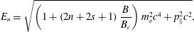 $$\begin{eqnarray}\displaystyle E_{n}=\sqrt{\left(1+\left(2n+2s+1\right)\frac{B}{B_{c}}\right)m_{e}^{2}c^{4}+p_{\Vert }^{2}c^{2}}, & & \displaystyle\end{eqnarray}$$
where
 $n$
represents the quantum number characterising the excitation degree of the level and
$n$
represents the quantum number characterising the excitation degree of the level and
 $s=\pm 1/2$
symbolises the electron spin (Daugherty & Ventura Reference Daugherty and Ventura1978). All energy levels are degenerated with an arbitrary choice of spin except for the fundamental level
$s=\pm 1/2$
symbolises the electron spin (Daugherty & Ventura Reference Daugherty and Ventura1978). All energy levels are degenerated with an arbitrary choice of spin except for the fundamental level
 $n=0$
for which
$n=0$
for which
 $s=-1/2$
. Actually, degeneracy is lifted through higher-order interactions between particles and the radiation field (Herold, Ruder & Wunner Reference Herold, Ruder and Wunner1982; Pavlov et al.
Reference Pavlov, Bezchastnov, Meszaros and Alexander1991). However, particles are free to move along magnetic field lines and need a parallel component of the electric field
$s=-1/2$
. Actually, degeneracy is lifted through higher-order interactions between particles and the radiation field (Herold, Ruder & Wunner Reference Herold, Ruder and Wunner1982; Pavlov et al.
Reference Pavlov, Bezchastnov, Meszaros and Alexander1991). However, particles are free to move along magnetic field lines and need a parallel component of the electric field
 $E_{\Vert }\neq 0$
in order to accelerate and radiate.
$E_{\Vert }\neq 0$
in order to accelerate and radiate.
Clearly
 $E_{\Vert }=0$
should not hold everywhere in the magnetosphere. We will come back to that point later when discussing possible gaps in the magnetosphere. As emphasized by Shibata (Reference Shibata1997), the determination of the accelerating electric field in the vacuum gaps should be treated as a global problem, including the current circuit flowing in the magnetosphere, as he did earlier in Shibata (Reference Shibata1991). Particle acceleration cannot be studied locally with special boundary conditions but consistently with the large-scale plasma configuration. Nevertheless, let us summarize the essential features of a pulsar magnetosphere so far
$E_{\Vert }=0$
should not hold everywhere in the magnetosphere. We will come back to that point later when discussing possible gaps in the magnetosphere. As emphasized by Shibata (Reference Shibata1997), the determination of the accelerating electric field in the vacuum gaps should be treated as a global problem, including the current circuit flowing in the magnetosphere, as he did earlier in Shibata (Reference Shibata1991). Particle acceleration cannot be studied locally with special boundary conditions but consistently with the large-scale plasma configuration. Nevertheless, let us summarize the essential features of a pulsar magnetosphere so far
-
(i) A plasma corotating with the star in ideal MHD or even the force-free approximation: solid body rotation dictated by the star and free motion along field lines.
-
(ii) A light cylinder: corotation stops outside this cylinder of radius
 $r_{L}=c/\unicode[STIX]{x1D6FA}$
. Particle inertia becomes important, magnetic field lines are significantly deformed and swept back by this mass load.
$r_{L}=c/\unicode[STIX]{x1D6FA}$
. Particle inertia becomes important, magnetic field lines are significantly deformed and swept back by this mass load. -
(iii) A magnetic topology with open and closed field lines. Closed field lines are imprisoned inside the light cylinder, plasma is corotating, no motion along field lines is permitted. Open field lines cross the surface of the light cylinder and their feet are anchored in the polar caps. Particles escape freely to infinity along these field lines.
-
(iv) A light surface: surface where the intensity of the electric field becomes equal to that of the magnetic field,
$E=cB$
. The electric drift approximation is violated, particles suffer acceleration, the ideal MHD or force-free approximation breaks down. The light surface and the light cylinder do not coincide, the first surface could be rejected to infinity for sufficiently strong longitudinal currents. -
(v) Polar caps: regions around the magnetic poles where open field lines are attached, deviation from the force-free approximation is expected to produce radio emission (Sturrock Reference Sturrock1971a ; Ruderman & Sutherland Reference Ruderman and Sutherland1975).
-
(vi) Slot gaps: small elongated excision volumes along the last closed field line within the magnetosphere, essentially empty of charges allowing pair creation (Arons & Scharlemann Reference Arons and Scharlemann1979; Arons Reference Arons1983), emergence of high-energy radiation and acceleration of particles (Dyks & Rudak Reference Dyks and Rudak2003).
-
(vii) For the aligned rotator, in the equatorial plane, transition from closed to open field lines goes through a so-called Y-type neutral point (for short Y-point) at a radius
$R_{Y}$
. It is generally assumed that
$R_{Y}=r_{L}$
but more generally it should satisfy
$R\leqslant R_{Y}\leqslant r_{L}$
. For instance Sturrock (Reference Sturrock1971b
) used the prescription
$R_{Y}=R^{1-\unicode[STIX]{x1D702}}r_{L}^{\unicode[STIX]{x1D702}}$
with
$\unicode[STIX]{x1D702}\in [0,1]$
. -
(viii) Outer gaps: large, almost empty, volumes in the magnetosphere, between the null surface (where
$\unicode[STIX]{x1D70C}=0$
) and the last closed field line with copious pair creation via
$\unicode[STIX]{x1D6FE}+\unicode[STIX]{x1D6FE}\rightarrow e^{+}+e^{-}$
(Cheng, Ho & Ruderman Reference Cheng, Ho and Ruderman1986a
,Reference Cheng, Ho and Ruderman
b
; Romani & Yadigaroglu Reference Romani and Yadigaroglu1995). Synchrotron emission from these gaps was studied by Crusius-Wätzel, Kunzl & Lesch (Reference Crusius-Wätzel, Kunzl and Lesch2001). -
(ix) Annular gaps: region between the critical field line and the null surface (Qiao et al. Reference Qiao, Lee, Wang, Xu and Han2004).


The scheme of figure 5 is an illustration of some important quantities introduced above. Possible finite temperature of the plasma is not accounted for but thermally supported hot magnetospheres were suggested by Henriksen & Rayburn (Reference Henriksen and Rayburn1974). Also, the situation outside the light cylinder is quite different from the regime inside it. Indeed, the pattern of charges and current distribution present outside the light cylinder are superluminal even if the particles themselves remain subluminal. Such motions generate radiation qualified as Schott radiation by da Costa & Kahn (Reference da Costa and Kahn1985) to be distinguished from Cerenkov radiation. A analogy with Cerenkov emission was nevertheless put forward by Ardavan (Reference Ardavan1981). This flow outside the light cylinder will be discussed along with pulsar wind theory § 7.
In a series of papers by Ardavan (Reference Ardavan1976a ,Reference Ardavan b ,Reference Ardavan c ,Reference Ardavan d ,Reference Ardavan e ) it was claimed that the transition between the corotating magnetosphere and the wind should go through a shock discontinuity and not via a continuous MHD flow. Singular surfaces in the magnetosphere were also found by Buckley (Reference Buckley1976).
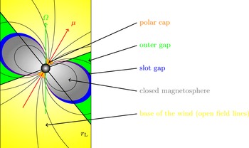
Figure 5. Schematic view of the magnetosphere within the light cylinder. Sizes of the gaps are not to scale.
3 Theory of pulsar magnetospheres
Establishing a consistent model of pulsar physics requires an accurate and quantitative description of the magnetospheric structure, the dynamics and radiative outputs, that is, the magnetic field topology, the current flowing inside and outside the light cylinder and particle acceleration mechanisms. Such a study in the general case is very difficult to conduct. Simple situations are instead treated but keeping the problem interesting from a physical point of view. The hypotheses usually accepted are the following
-
(i) The magnetosphere is filled with a pair plasma screening the electric field such that
$\boldsymbol{E}\boldsymbol{\cdot }\boldsymbol{B}=0$
everywhere. This means that all charged particles adapt their motion to maintain a vanishing acceleration along field lines, thus
$E_{\Vert }=0$
. Spatially localized slight deviations from this rigorous
$E_{\Vert }=0$
fulfilment are expected to ignite electromagnetic activity in the magnetosphere. Subtleties in achieving
$E_{\Vert }\neq 0$
lead to different plasma regimes involving a plethora of gap and cap models. -
(ii) Particles follow an electric drift motion superposed to a translation along field lines.
-
(iii) The regime is stationary and at least for earlier models assumed axisymmetric (aligned rotator).
-
(iv) Primary particles emanate from the surface of the star, there is no pair creation.
-
(v) The plasma is quasi-neutral, which means that the space charge is overwhelmed by a background of much more dense neutral plasma.
-
(vi) Sometimes the opposite is claimed, that is a plasma entirely charge separated, in other words, a truly non-neutral plasma.
-
(vii) Gravity and pressure (temperature) forces are neglected compared to electromagnetic forces.


Let us explain in more detail important implications of all these assumptions.
3.1 Filled magnetospheric model
An aligned rotator in vacuum does not radiate because dipolar magnetic emission cancels for zero obliquity,
 $\unicode[STIX]{x1D712}=0$
. But if plasma cohabits within the magnetosphere, the current generated by the plasma motion induces a braking of the star through torques exerted on the stellar crust. This idea was formulated by Goldreich & Julian (Reference Goldreich and Julian1969). But where does this plasma come from? At first sight, the gravitational field is sufficiently intense to retain particles at its surface but nevertheless this hypothesis is wrong. Indeed, the strong magnetic field combined with the rotation of the star generates a potential drop at the stellar surface hardly sustainable for the charges in the crust. The electric field component aligned with the magnetic field, of the order of
$\unicode[STIX]{x1D712}=0$
. But if plasma cohabits within the magnetosphere, the current generated by the plasma motion induces a braking of the star through torques exerted on the stellar crust. This idea was formulated by Goldreich & Julian (Reference Goldreich and Julian1969). But where does this plasma come from? At first sight, the gravitational field is sufficiently intense to retain particles at its surface but nevertheless this hypothesis is wrong. Indeed, the strong magnetic field combined with the rotation of the star generates a potential drop at the stellar surface hardly sustainable for the charges in the crust. The electric field component aligned with the magnetic field, of the order of
 $E_{\Vert }\approx 10^{10}$
Vm
$E_{\Vert }\approx 10^{10}$
Vm
 $^{-1}$
, is able to pull them out. The discontinuity of
$^{-1}$
, is able to pull them out. The discontinuity of
 $E_{r}$
when crossing the surface–vacuum interface provokes a surface charge density constrained to spread over the vacuum because of
$E_{r}$
when crossing the surface–vacuum interface provokes a surface charge density constrained to spread over the vacuum because of
 $E_{\Vert }\neq 0$
. Comparing the Coulomb force to the gravitational attraction for a proton, we estimate the ratio
$E_{\Vert }\neq 0$
. Comparing the Coulomb force to the gravitational attraction for a proton, we estimate the ratio
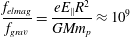 $$\begin{eqnarray}\displaystyle \frac{f_{elmag}}{f_{grav}}=\frac{eE_{\Vert }R^{2}}{GMm_{p}}\approx 10^{9} & & \displaystyle\end{eqnarray}$$
and a value
 $m_{e}/m_{p}\approx 2000$
larger for electrons. The gravitational force is completely negligible. The vacuum around the star is unstable and must replenish with charge.
$m_{e}/m_{p}\approx 2000$
larger for electrons. The gravitational force is completely negligible. The vacuum around the star is unstable and must replenish with charge.
Goldreich & Julian (Reference Goldreich and Julian1969) supposed that the electromagnetic environment of the magnetosphere is described by a plasma corotating with the star up to the light cylinder and magnetic field lines with no toroidal component. A fundamental difference exists between closed and open field lines. In the latter case, a current circulation is launched from the polar caps, regions with a cone opening angle given by simple geometrical arguments in (3.10). Unfortunately, estimation of the energy loss by magnetodipole radiation furnishes the same order of magnitude as the Deutsch–Pacini model. It is therefore impossible to assess which of both models, with an empty or fully filled magnetosphere, is really pertinent for pulsars.
The light cylinder is an imaginary cylindrical surface whose axis is parallel to the rotation axis of the star and it possesses a radius corresponding to the distance from the centre of the neutron star at which the corotation speed reaches the speed of light. The radius of the light cylinder is thus defined by
 $$\begin{eqnarray}\displaystyle r_{L}=\frac{c}{\unicode[STIX]{x1D6FA}}. & & \displaystyle\end{eqnarray}$$
Physically, corotation is insured by the drift motion of particles in the electromagnetic field at the electric drift velocity given by
 $$\begin{eqnarray}\displaystyle \boldsymbol{v}_{Edrift}=\frac{\boldsymbol{E}\wedge \boldsymbol{B}}{B^{2}}. & & \displaystyle\end{eqnarray}$$
It does not depend on the nature of the particles (mass, charge) but uniquely on the structure of the electromagnetic field
 $(\boldsymbol{E},\boldsymbol{B})$
. Therefore, this electric drift cannot induce any current except if there is a deviation from charge neutrality whereby a convective current exists. This drift does not forbid motion along magnetic field lines. Indeed, for a perfectly conducting plasma, in the ideal MHD regime, the drift speed according to (2.6) becomes
$(\boldsymbol{E},\boldsymbol{B})$
. Therefore, this electric drift cannot induce any current except if there is a deviation from charge neutrality whereby a convective current exists. This drift does not forbid motion along magnetic field lines. Indeed, for a perfectly conducting plasma, in the ideal MHD regime, the drift speed according to (2.6) becomes
 $$\begin{eqnarray}\displaystyle \boldsymbol{v}_{Edrift}=\unicode[STIX]{x1D734}\wedge \boldsymbol{r}-\frac{\boldsymbol{B}\boldsymbol{\cdot }(\unicode[STIX]{x1D734}\wedge \boldsymbol{r})}{B^{2}}\boldsymbol{B}, & & \displaystyle\end{eqnarray}$$
which clearly indicates a contribution from corotation recognizable in the first term on the right-hand side, plus a sliding along field lines recognizable in the second term on the right-hand side. In order to avoid exceeding the speed of light, field lines have to bend to induce a toroidal component
 $B_{\unicode[STIX]{x1D711}}\neq 0$
. This points out the dichotomy between closed and open field lines. The fundamental problem of pulsar electrodynamics was to find a reasonable expression for this parallel current. Numerical simulations have been able to answer satisfactorily this question as we discuss in § 5. Asseo, Beaufils & Pellat (Reference Asseo, Beaufils and Pellat1984) considered interesting alternative models carefully by studying the force-free surfaces. They attempted also to include vacuum gaps between the neutron star and the force-free regions as well as particle exchange via charged polar beams. Lyubarsky (Reference Lyubarsky2012) noticed that the current required to flow within the magnetosphere does not necessarily match the pair production rate and its flow within the polar caps. The mismatch could induce modulation of radio emission.
$B_{\unicode[STIX]{x1D711}}\neq 0$
. This points out the dichotomy between closed and open field lines. The fundamental problem of pulsar electrodynamics was to find a reasonable expression for this parallel current. Numerical simulations have been able to answer satisfactorily this question as we discuss in § 5. Asseo, Beaufils & Pellat (Reference Asseo, Beaufils and Pellat1984) considered interesting alternative models carefully by studying the force-free surfaces. They attempted also to include vacuum gaps between the neutron star and the force-free regions as well as particle exchange via charged polar beams. Lyubarsky (Reference Lyubarsky2012) noticed that the current required to flow within the magnetosphere does not necessarily match the pair production rate and its flow within the polar caps. The mismatch could induce modulation of radio emission.
3.2 Ideal MHD and force-free limit
In this most studied approximation, the magnetosphere is sufficiently populated with plasma in order for the conductivity in the medium to become infinite, or in other words, that all components of the electric field parallel to the magnetic field to be immediately screened,
 $E_{\Vert }=0$
. Moreover, the electromagnetic field dominates the dynamics of the magnetosphere to several orders of magnitude with respect to pressure, gravity and inertia. The Lorentz force on a plasma element, treated as a one-component fluid, is therefore null. Its vanishing leads to the so-called force-free approximation
$E_{\Vert }=0$
. Moreover, the electromagnetic field dominates the dynamics of the magnetosphere to several orders of magnitude with respect to pressure, gravity and inertia. The Lorentz force on a plasma element, treated as a one-component fluid, is therefore null. Its vanishing leads to the so-called force-free approximation
 $$\begin{eqnarray}\displaystyle \unicode[STIX]{x1D70C}_{e}\boldsymbol{E}+\boldsymbol{j}\wedge \boldsymbol{B}=0, & & \displaystyle\end{eqnarray}$$
where
 $\unicode[STIX]{x1D70C}_{e}$
is the charge density and
$\unicode[STIX]{x1D70C}_{e}$
is the charge density and
 $\boldsymbol{j}$
the current density. The electric field is orthogonal to the magnetic field
$\boldsymbol{j}$
the current density. The electric field is orthogonal to the magnetic field
 $\boldsymbol{E}\boldsymbol{\cdot }\boldsymbol{B}=0$
. Implicitly, magnetic energy density
$\boldsymbol{E}\boldsymbol{\cdot }\boldsymbol{B}=0$
. Implicitly, magnetic energy density
 $B^{2}/2\unicode[STIX]{x1D707}_{0}$
dominates against any other kind of energy and notably the one related to particle inertia. This corresponds to the vanishing mass limit. Moreover, no dissipation is associated with this regime, ideal MHD applies to the flow of velocity field
$B^{2}/2\unicode[STIX]{x1D707}_{0}$
dominates against any other kind of energy and notably the one related to particle inertia. This corresponds to the vanishing mass limit. Moreover, no dissipation is associated with this regime, ideal MHD applies to the flow of velocity field
 $\boldsymbol{v}$
and
$\boldsymbol{v}$
and
 $$\begin{eqnarray}\displaystyle \boldsymbol{E}+\boldsymbol{v}\wedge \boldsymbol{B}=0. & & \displaystyle\end{eqnarray}$$
From (3.5) and (3.6) we deduce that the current density is made of a convective term related to charge separation
 $\unicode[STIX]{x1D70C}_{e}\boldsymbol{v}$
and to a field aligned current
$\unicode[STIX]{x1D70C}_{e}\boldsymbol{v}$
and to a field aligned current
 $j_{\Vert }$
thus
$j_{\Vert }$
thus
 $$\begin{eqnarray}\displaystyle \boldsymbol{j}=\unicode[STIX]{x1D70C}_{e}\boldsymbol{v}+j_{\Vert }\boldsymbol{B}/B. & & \displaystyle\end{eqnarray}$$

Figure 6. First model of a pulsar magnetosphere as proposed by Goldreich & Julian (Reference Goldreich and Julian1969). The neutron star is symbolized by a circle on the bottom left. The open field lines let a charged wind escape from the poles. The closed field lines are filled with the corotation density and do not support any electric current.
Goldreich & Julian (Reference Goldreich and Julian1969) postulated simply that the magnetosphere was entirely filled up to the light cylinder, figure 6. The magnetic field
 $\boldsymbol{B}$
aligned with the magnetic moment
$\boldsymbol{B}$
aligned with the magnetic moment
 $\unicode[STIX]{x1D741}$
and rotating at angular speed
$\unicode[STIX]{x1D741}$
and rotating at angular speed
 $\unicode[STIX]{x1D734}$
, generates an electromotive field from which forces are sufficient to overcome gravity, creating a magnetosphere filled with plasma ejected from the surface of the star. In the aligned case evoked here, magnetic dipolar emission, as suggested by Pacini (Reference Pacini1968), disappears, there is no more braking through magnetodipole radiation but through acceleration of charges in the magnetosphere, as explained later. If we assume that the reservoir of particles is infinite, the magnetosphere will be entirely saturated with ions and electrons up to the light cylinder with a density of charge insuring corotation of the whole system according to the Maxwell–Gauss equation
$\unicode[STIX]{x1D734}$
, generates an electromotive field from which forces are sufficient to overcome gravity, creating a magnetosphere filled with plasma ejected from the surface of the star. In the aligned case evoked here, magnetic dipolar emission, as suggested by Pacini (Reference Pacini1968), disappears, there is no more braking through magnetodipole radiation but through acceleration of charges in the magnetosphere, as explained later. If we assume that the reservoir of particles is infinite, the magnetosphere will be entirely saturated with ions and electrons up to the light cylinder with a density of charge insuring corotation of the whole system according to the Maxwell–Gauss equation
 $$\begin{eqnarray}\displaystyle \unicode[STIX]{x1D70C}_{e}=\unicode[STIX]{x1D700}_{0}\unicode[STIX]{x1D735}\boldsymbol{\cdot }\boldsymbol{E}=\unicode[STIX]{x1D70C}_{cor}+\boldsymbol{j}\boldsymbol{\cdot }(\unicode[STIX]{x1D734}\wedge \boldsymbol{r})/c^{2}. & & \displaystyle\end{eqnarray}$$
The corotation charge density is given by
 $\unicode[STIX]{x1D70C}_{cor}=-2\unicode[STIX]{x1D700}_{0}\unicode[STIX]{x1D734}\boldsymbol{\cdot }\boldsymbol{B}$
with the associated particle density number
$\unicode[STIX]{x1D70C}_{cor}=-2\unicode[STIX]{x1D700}_{0}\unicode[STIX]{x1D734}\boldsymbol{\cdot }\boldsymbol{B}$
with the associated particle density number
 $n_{cor}=\unicode[STIX]{x1D70C}_{cor}/e$
.
$n_{cor}=\unicode[STIX]{x1D70C}_{cor}/e$
.
 $\unicode[STIX]{x1D70C}_{cor}$
is the density required to screen the longitudinal electric field. If the current density is purely corotating then
$\unicode[STIX]{x1D70C}_{cor}$
is the density required to screen the longitudinal electric field. If the current density is purely corotating then
 $\boldsymbol{j}=\unicode[STIX]{x1D70C}_{e}\unicode[STIX]{x1D734}\wedge \boldsymbol{r}$
and the density simplifies into
$\boldsymbol{j}=\unicode[STIX]{x1D70C}_{e}\unicode[STIX]{x1D734}\wedge \boldsymbol{r}$
and the density simplifies into
 $$\begin{eqnarray}\displaystyle \unicode[STIX]{x1D70C}_{e}=\frac{\unicode[STIX]{x1D70C}_{cor}}{1-(\unicode[STIX]{x1D734}\wedge \boldsymbol{r})^{2}/c^{2}}. & & \displaystyle\end{eqnarray}$$
In that case, the density diverges at the light cylinder unless
 $\unicode[STIX]{x1D734}\boldsymbol{\cdot }\boldsymbol{B}=0$
there. The ideal MHD or force-free approximation requires a particle density number much larger than the minimum required by the corotation, that is
$\unicode[STIX]{x1D734}\boldsymbol{\cdot }\boldsymbol{B}=0$
there. The ideal MHD or force-free approximation requires a particle density number much larger than the minimum required by the corotation, that is
 $n\gg n_{cor}$
to insure almost perfect charge neutrality. Thus if pair creation is ineffective, such high densities could not be reached and the neutral fluid regime should be replaced by a non-neutral plasma behaviour. The denominator of (3.9) brings in a relativistic correction in
$n\gg n_{cor}$
to insure almost perfect charge neutrality. Thus if pair creation is ineffective, such high densities could not be reached and the neutral fluid regime should be replaced by a non-neutral plasma behaviour. The denominator of (3.9) brings in a relativistic correction in
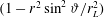 $(1-r^{2}\sin ^{2}\unicode[STIX]{x1D717}/r_{L}^{2})$
due to the magnetospheric currents modifying the structure of the magnetic field. A phenomenon very perceptible in the vicinity of the light cylinder. Indeed, corotation of the magnetospheric charge with the pulsar generates an electric current
$(1-r^{2}\sin ^{2}\unicode[STIX]{x1D717}/r_{L}^{2})$
due to the magnetospheric currents modifying the structure of the magnetic field. A phenomenon very perceptible in the vicinity of the light cylinder. Indeed, corotation of the magnetospheric charge with the pulsar generates an electric current
 $\boldsymbol{j}=\unicode[STIX]{x1D70C}_{e}\boldsymbol{v}$
which modifies the initial configuration of the magnetic field. This self-consistent current leads to more important effects when approaching the light cylinder. It is responsible for certain relativistic effects, in particular the determination of the corotation density. The magnetic perturbations induced by these corotating currents have a tendency to repel field lines in a direction opposite to the pulsar (the plasma diamagnetic effect). These far away field lines inflate to infinity until they open up. Mass loading causes field lines to sweep back, thus generating a longitudinal current
$\boldsymbol{j}=\unicode[STIX]{x1D70C}_{e}\boldsymbol{v}$
which modifies the initial configuration of the magnetic field. This self-consistent current leads to more important effects when approaching the light cylinder. It is responsible for certain relativistic effects, in particular the determination of the corotation density. The magnetic perturbations induced by these corotating currents have a tendency to repel field lines in a direction opposite to the pulsar (the plasma diamagnetic effect). These far away field lines inflate to infinity until they open up. Mass loading causes field lines to sweep back, thus generating a longitudinal current
 $j_{\Vert }$
that is difficult to estimate solely on first principles.
$j_{\Vert }$
that is difficult to estimate solely on first principles.
The magnetosphere then splits into two regions, one with closed field lines and the other with open field lines. Both kinds of field lines are in solid body rotation. Brought back to the level of the stellar surface, open field lines focus into a small zone in the vicinity of the magnetic poles, the polar caps which have a radius not larger than
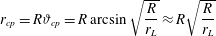 $$\begin{eqnarray}\displaystyle r_{cp}=R\unicode[STIX]{x1D717}_{cp}=R\arcsin \sqrt{\frac{R}{r_{L}}}\approx R\sqrt{\frac{R}{r_{L}}} & & \displaystyle\end{eqnarray}$$
assuming vacuum dipolar field lines whose polar equation is
 $r=\unicode[STIX]{x1D706}\sin ^{2}\unicode[STIX]{x1D717}$
. These estimates do not include distortion due to either retardation effects around the light cylinder and already present in the Deutsch solution or magnetospheric currents. The region enclosed inside the light cylinder is entirely filled with plasma at the corotation density
$r=\unicode[STIX]{x1D706}\sin ^{2}\unicode[STIX]{x1D717}$
. These estimates do not include distortion due to either retardation effects around the light cylinder and already present in the Deutsch solution or magnetospheric currents. The region enclosed inside the light cylinder is entirely filled with plasma at the corotation density
 $\unicode[STIX]{x1D70C}_{e}$
. If the intrinsic magnetic field is dipolar, positively charged regions are separated from negatively charged regions by a conical interface with opening angle defined by the condition
$\unicode[STIX]{x1D70C}_{e}$
. If the intrinsic magnetic field is dipolar, positively charged regions are separated from negatively charged regions by a conical interface with opening angle defined by the condition
 $\unicode[STIX]{x1D734}\boldsymbol{\cdot }\boldsymbol{B}=0$
according to (3.9). Some magnetic field lines enclose simultaneously charges of both signs, which raises the question of the existence of a process able to explain how this transport can be produced. Open magnetic field lines going beyond the light cylinder let particles definitely escape from the pulsar, contributing to the total electric current. They are divided into electron supported flow and proton supported flow, delimited by the critical field line which is at the same electric potential as the interstellar medium. The star loses then charge from the polar caps through the formation of a charged wind which is a situation that cannot last for ever. The power released by these escaping particles is comparable to the power radiated by the magnetic dipole of Pacini (Reference Pacini1968). The characteristic braking time scale and pulsar age will then remain the same. Quantitative results will be discussed in the paragraph about numerical simulations in § 5. Note that in some versions of the Goldreich & Julian (Reference Goldreich and Julian1969) model, electron–positron pairs are formed during the period of magnetosphere filling. Positive charges are then made of positrons.
$\unicode[STIX]{x1D734}\boldsymbol{\cdot }\boldsymbol{B}=0$
according to (3.9). Some magnetic field lines enclose simultaneously charges of both signs, which raises the question of the existence of a process able to explain how this transport can be produced. Open magnetic field lines going beyond the light cylinder let particles definitely escape from the pulsar, contributing to the total electric current. They are divided into electron supported flow and proton supported flow, delimited by the critical field line which is at the same electric potential as the interstellar medium. The star loses then charge from the polar caps through the formation of a charged wind which is a situation that cannot last for ever. The power released by these escaping particles is comparable to the power radiated by the magnetic dipole of Pacini (Reference Pacini1968). The characteristic braking time scale and pulsar age will then remain the same. Quantitative results will be discussed in the paragraph about numerical simulations in § 5. Note that in some versions of the Goldreich & Julian (Reference Goldreich and Julian1969) model, electron–positron pairs are formed during the period of magnetosphere filling. Positive charges are then made of positrons.
Although being able to explain the origin of the particles, this model suffers from internal inconsistency problems bound to the endless discharge of the pulsar and to the thorny issue of the current closure. Moreover, Smith, Michel & Thacker (Reference Smith, Michel and Thacker2001) have demonstrated through numerical simulations that this model of the magnetosphere entirely filled with corotating plasma is unstable. They observed a collapse to a new charge distribution similar to the one obtained by Krause-Polstorff & Michel (Reference Krause-Polstorff and Michel1985b ), see § 6 which discusses the electrosphere. We note that the electric field produced in vacuum by a rotating star is known since the work by Davis (Reference Davis1947) and for the oblique rotator filled with plasma since Hones & Bergeson (Reference Hones and Bergeson1965), and thus well before Goldreich & Julian (Reference Goldreich and Julian1969). Whether the force-free solution can strictly apply outside the light cylinder or not was questioned by Buckley (Reference Buckley1978), who showed that a small parallel electric field must exist in order to allow for a finite speed of particles along field lines.
3.3 The pulsar equation
The current flowing along magnetic field lines in the magnetosphere constitutes an inescapable unknown of the dynamics of pulsars. In order to determine it self-consistently, the problem has to be solved from the surface of the star up to infinity. This task is very arduous but real progress has been made over the last decade thanks to numerical simulations. But before discussing this, let us note the main approaches before this new era of informatics. Michel (Reference Michel1973a
) was the first to compute the exact structure of a 2-D axisymmetric magnetosphere in the absence of a field aligned current,
 $j_{\Vert }=0$
. The fundamental equation for these corotating field lines was given through the magnetic flux function
$j_{\Vert }=0$
. The fundamental equation for these corotating field lines was given through the magnetic flux function
 $\unicode[STIX]{x1D713}$
related to the magnetic field by
$\unicode[STIX]{x1D713}$
related to the magnetic field by
 $\boldsymbol{B}=1/r\unicode[STIX]{x1D735}\unicode[STIX]{x1D713}\wedge \boldsymbol{e}_{\unicode[STIX]{x1D711}}$
. The magnetic flux function
$\boldsymbol{B}=1/r\unicode[STIX]{x1D735}\unicode[STIX]{x1D713}\wedge \boldsymbol{e}_{\unicode[STIX]{x1D711}}$
. The magnetic flux function
 $\unicode[STIX]{x1D713}$
, in the presence of a longitudinal current, satisfies a relation established independently by Scharlemann & Wagoner (Reference Scharlemann and Wagoner1973) and by Michel (Reference Michel1973b
) see also Julian (Reference Julian1973). It is written as
$\unicode[STIX]{x1D713}$
, in the presence of a longitudinal current, satisfies a relation established independently by Scharlemann & Wagoner (Reference Scharlemann and Wagoner1973) and by Michel (Reference Michel1973b
) see also Julian (Reference Julian1973). It is written as
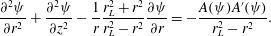 $$\begin{eqnarray}\displaystyle \frac{\unicode[STIX]{x2202}^{2}\unicode[STIX]{x1D713}}{\unicode[STIX]{x2202}r^{2}}+\frac{\unicode[STIX]{x2202}^{2}\unicode[STIX]{x1D713}}{\unicode[STIX]{x2202}z^{2}}-\frac{1}{r}\frac{r_{L}^{2}+r^{2}}{r_{L}^{2}-r^{2}}\frac{\unicode[STIX]{x2202}\unicode[STIX]{x1D713}}{\unicode[STIX]{x2202}r}=-\frac{A(\unicode[STIX]{x1D713})A^{\prime }(\unicode[STIX]{x1D713})}{r_{L}^{2}-r^{2}}. & & \displaystyle\end{eqnarray}$$
It is often named the pulsar equation. Endean (Reference Endean1974) gave another derivation of the pulsar equation and made some useful comments about the underlying hypothesis. The function
 $A(\unicode[STIX]{x1D713})$
is a priori arbitrary, but it must verify some Alfvénic regularity conditions at the light cylinder. It is related to the poloidal current
$A(\unicode[STIX]{x1D713})$
is a priori arbitrary, but it must verify some Alfvénic regularity conditions at the light cylinder. It is related to the poloidal current
 $I$
by
$I$
by
 $\unicode[STIX]{x1D707}_{0}I=2\unicode[STIX]{x03C0}A$
. The singularity at
$\unicode[STIX]{x1D707}_{0}I=2\unicode[STIX]{x03C0}A$
. The singularity at
 $r=r_{L}$
imposes a strong constraint on the function
$r=r_{L}$
imposes a strong constraint on the function
 $A$
that must satisfy the regularity condition
$A$
that must satisfy the regularity condition
 $2r_{L}\unicode[STIX]{x2202}\unicode[STIX]{x1D713}/\unicode[STIX]{x2202}r=AA^{\prime }$
. In the absence of longitudinal currents
$2r_{L}\unicode[STIX]{x2202}\unicode[STIX]{x1D713}/\unicode[STIX]{x2202}r=AA^{\prime }$
. In the absence of longitudinal currents
 $A=0$
and far away from the light cylinder,
$A=0$
and far away from the light cylinder,
 $r\ll r_{L}$
, the multipolar expansion of the field in a vacuum is retrieved. Note also that this equation is singular on the light cylinder
$r\ll r_{L}$
, the multipolar expansion of the field in a vacuum is retrieved. Note also that this equation is singular on the light cylinder
 $r=r_{L}$
. It can be shown that these field lines are perpendicular to the light cylinder. This leads to a very important physical conclusion: the Poynting vector does not possess a component normal to the light cylinder, which means that the electromagnetic energy flux through the light cylinder vanishes. In the absence of a longitudinal current, the plasma filling the magnetosphere screens the dipolar field, no magnetodipole emission is allowed. The energy loss of the pulsar cannot come from the action of a current circulating in the interior of its magnetosphere without crossing the light cylinder. Moreover, the solution exterior to the light cylinder has no influence on the interior solution. Solving (3.11) for the flux function
$r=r_{L}$
. It can be shown that these field lines are perpendicular to the light cylinder. This leads to a very important physical conclusion: the Poynting vector does not possess a component normal to the light cylinder, which means that the electromagnetic energy flux through the light cylinder vanishes. In the absence of a longitudinal current, the plasma filling the magnetosphere screens the dipolar field, no magnetodipole emission is allowed. The energy loss of the pulsar cannot come from the action of a current circulating in the interior of its magnetosphere without crossing the light cylinder. Moreover, the solution exterior to the light cylinder has no influence on the interior solution. Solving (3.11) for the flux function
 $\unicode[STIX]{x1D713}$
, Michel (Reference Michel1973a
) obtained the shape of the magnetic field interior to the light cylinder. The plasma has a tendency to deform field lines in the direction of an increase of total magnetic flux extending to the light cylinder. Magnetic energy in the vicinity of the cylinder is also increased. Mestel, Phillips & Wang (Reference Mestel, Phillips and Wang1979) and Mestel & Wang (Reference Mestel and Wang1979) extended this model by adding small gaps between ions and electrons along the null surface. Perturbations of this null surface by, for instance, charge depletion in the charge separated plasma is unstable against vacuum gap formation in its vicinity. Following arguments detailed by Holloway (Reference Holloway1973), replenishment is forbidden. Later Holloway & Pryce (Reference Holloway and Pryce1981) studied the properties of vacuum gaps with finite temperature plasmas. A current flows out of the null surface where replenishment is impossible but acceleration of particles to very high energies is expected in the huge potential drop limited by pair production (Cheng, Ruderman & Sutherland Reference Cheng, Ruderman and Sutherland1976). Okamoto (Reference Okamoto1974, Reference Okamoto1975) suppressed the hypothesis of corotation introduced by Michel (Reference Michel1973a
) and computed the magnetic field configuration in such a situation. Scharlemann & Wagoner (Reference Scharlemann and Wagoner1973) introduced particle inertia but assumed that it remains small and did not give exact solutions. Inertial effects were also the topic of Schmalz, Ruder & Herold (Reference Schmalz, Ruder and Herold1979) who presented first results in Schmalz et al. (Reference Schmalz, Ruder, Herold and Rossmanith1980). The problem of an oblique rotator has not been studied. Let us cite the work by Mestel, Panagi & Shibata (Reference Mestel, Panagi and Shibata1999) who determined the pulsar magnetosphere in the case of a perpendicular rotator. They reproduced a special case of the results preserved by Beskin, Gurevich & Istomin (Reference Beskin, Gurevich and Istomin1983) who obtained solutions for arbitrary inclination angle. The current formed no only by the particle flow but also the displacement current act to distort field lines.
$\unicode[STIX]{x1D713}$
, Michel (Reference Michel1973a
) obtained the shape of the magnetic field interior to the light cylinder. The plasma has a tendency to deform field lines in the direction of an increase of total magnetic flux extending to the light cylinder. Magnetic energy in the vicinity of the cylinder is also increased. Mestel, Phillips & Wang (Reference Mestel, Phillips and Wang1979) and Mestel & Wang (Reference Mestel and Wang1979) extended this model by adding small gaps between ions and electrons along the null surface. Perturbations of this null surface by, for instance, charge depletion in the charge separated plasma is unstable against vacuum gap formation in its vicinity. Following arguments detailed by Holloway (Reference Holloway1973), replenishment is forbidden. Later Holloway & Pryce (Reference Holloway and Pryce1981) studied the properties of vacuum gaps with finite temperature plasmas. A current flows out of the null surface where replenishment is impossible but acceleration of particles to very high energies is expected in the huge potential drop limited by pair production (Cheng, Ruderman & Sutherland Reference Cheng, Ruderman and Sutherland1976). Okamoto (Reference Okamoto1974, Reference Okamoto1975) suppressed the hypothesis of corotation introduced by Michel (Reference Michel1973a
) and computed the magnetic field configuration in such a situation. Scharlemann & Wagoner (Reference Scharlemann and Wagoner1973) introduced particle inertia but assumed that it remains small and did not give exact solutions. Inertial effects were also the topic of Schmalz, Ruder & Herold (Reference Schmalz, Ruder and Herold1979) who presented first results in Schmalz et al. (Reference Schmalz, Ruder, Herold and Rossmanith1980). The problem of an oblique rotator has not been studied. Let us cite the work by Mestel, Panagi & Shibata (Reference Mestel, Panagi and Shibata1999) who determined the pulsar magnetosphere in the case of a perpendicular rotator. They reproduced a special case of the results preserved by Beskin, Gurevich & Istomin (Reference Beskin, Gurevich and Istomin1983) who obtained solutions for arbitrary inclination angle. The current formed no only by the particle flow but also the displacement current act to distort field lines.
Progress was made by Contopoulos, Kazanas & Fendt (Reference Contopoulos, Kazanas and Fendt1999) who managed to treat numerically the regular singularity along the light cylinder. According to their results, it seems that only one such function
 $A$
exists for which the solution crossing the light cylinder possess no discontinuity. However, other solutions have been found by Timokhin (Reference Timokhin2006) if the singular point is located inside the light cylinder, translating the Y-point
$A$
exists for which the solution crossing the light cylinder possess no discontinuity. However, other solutions have been found by Timokhin (Reference Timokhin2006) if the singular point is located inside the light cylinder, translating the Y-point
 $R_{Y}$
as proposed by Sturrock (Reference Sturrock1971b
). Equating the force balance between the Y-point and the centrifugal force Roberts & Sturrock (Reference Roberts and Sturrock1972) found a braking index of
$R_{Y}$
as proposed by Sturrock (Reference Sturrock1971b
). Equating the force balance between the Y-point and the centrifugal force Roberts & Sturrock (Reference Roberts and Sturrock1972) found a braking index of
 $n=7/3$
for the Crab, in agreement with observation at that time and also in agreement with the period–pulse width relation. Closed field lines do not necessarily stop at the light cylinder but may already be well within it, at the so called force-balance radius where gravitational and centrifugal forces compensate each other (Roberts & Sturrock Reference Roberts and Sturrock1973). As pulsars spin down, the Y-point moves outwards at a rate depending on reconnection efficiency, the two extreme cases being, on one hand, no shift, thus
$n=7/3$
for the Crab, in agreement with observation at that time and also in agreement with the period–pulse width relation. Closed field lines do not necessarily stop at the light cylinder but may already be well within it, at the so called force-balance radius where gravitational and centrifugal forces compensate each other (Roberts & Sturrock Reference Roberts and Sturrock1973). As pulsars spin down, the Y-point moves outwards at a rate depending on reconnection efficiency, the two extreme cases being, on one hand, no shift, thus
 $R_{Y}=cst$
and on the other hand, very efficient readjustment of the magnetic topology leading to
$R_{Y}=cst$
and on the other hand, very efficient readjustment of the magnetic topology leading to
 $R_{Y}=r_{L}$
. This could have interesting implications for the death line of pulsars (Contopoulos & Spitkovsky Reference Contopoulos and Spitkovsky2006). Wherever the location of the Y-point, the circuit must be closed by a return current. The path taken by this return current may be along the last open field lines, the so-called separatrix, but not necessarily. Indeed the dynamics of this Y-point, even only described locally, is still delicate and controversial. In addition, it is not clear how it influences the global structure of the magnetosphere (Uzdensky Reference Uzdensky2003). The solution found by Contopoulos et al. (Reference Contopoulos, Kazanas and Fendt1999) is not unique. The delicate point concerns the current sheet in the equatorial plane that was introduced, so to say, by hand in order to provide the current closure of the electric circuit. In an attempt to remove this arbitrariness of the current sheet, Contopoulos, Kalapotharakos & Kazanas (Reference Contopoulos, Kalapotharakos and Kazanas2014) constructed another force-free solution for the axisymmetric rotator that takes off the separatrix. The current sheet only exists outside the light cylinder, starting at the Y-point. Dissipation occurs only in this current sheet which obeys to a different dynamics compared to the standard pressure supported discontinuity. Particle acceleration in the radiation reaction limit can effectively dissipate the Poynting flux within this current sheet (Contopoulos Reference Contopoulos2016b
). A disk wind and jet geometry completely removing the current sheet in all space is also not excluded (Sulkanen & Lovelace Reference Sulkanen and Lovelace1990; Lovelace, Turner & Romanova Reference Lovelace, Turner and Romanova2006). As these authors emphasized, such kinds of solutions are also not unique. The current sheet problem instigated Ogura & Kojima (Reference Ogura and Kojima2003) to look deeper into the force-free and MHD solutions of an axisymmetric rotator. They showed that the drift approximation is violated at several light-cylinder radii. See also Takamori et al. (Reference Takamori, Okawa, Takamoto and Suwa2014) for another method to construct current sheet free magnetospheres. In any case, the pulsar generates an electric current originating from the polar caps. By action of the Laplace force on the stellar crust, it brakes its rotation. The separatrix is also a privileged place to produce the observed pulsed emission (Gruzinov Reference Gruzinov2007).
$R_{Y}=r_{L}$
. This could have interesting implications for the death line of pulsars (Contopoulos & Spitkovsky Reference Contopoulos and Spitkovsky2006). Wherever the location of the Y-point, the circuit must be closed by a return current. The path taken by this return current may be along the last open field lines, the so-called separatrix, but not necessarily. Indeed the dynamics of this Y-point, even only described locally, is still delicate and controversial. In addition, it is not clear how it influences the global structure of the magnetosphere (Uzdensky Reference Uzdensky2003). The solution found by Contopoulos et al. (Reference Contopoulos, Kazanas and Fendt1999) is not unique. The delicate point concerns the current sheet in the equatorial plane that was introduced, so to say, by hand in order to provide the current closure of the electric circuit. In an attempt to remove this arbitrariness of the current sheet, Contopoulos, Kalapotharakos & Kazanas (Reference Contopoulos, Kalapotharakos and Kazanas2014) constructed another force-free solution for the axisymmetric rotator that takes off the separatrix. The current sheet only exists outside the light cylinder, starting at the Y-point. Dissipation occurs only in this current sheet which obeys to a different dynamics compared to the standard pressure supported discontinuity. Particle acceleration in the radiation reaction limit can effectively dissipate the Poynting flux within this current sheet (Contopoulos Reference Contopoulos2016b
). A disk wind and jet geometry completely removing the current sheet in all space is also not excluded (Sulkanen & Lovelace Reference Sulkanen and Lovelace1990; Lovelace, Turner & Romanova Reference Lovelace, Turner and Romanova2006). As these authors emphasized, such kinds of solutions are also not unique. The current sheet problem instigated Ogura & Kojima (Reference Ogura and Kojima2003) to look deeper into the force-free and MHD solutions of an axisymmetric rotator. They showed that the drift approximation is violated at several light-cylinder radii. See also Takamori et al. (Reference Takamori, Okawa, Takamoto and Suwa2014) for another method to construct current sheet free magnetospheres. In any case, the pulsar generates an electric current originating from the polar caps. By action of the Laplace force on the stellar crust, it brakes its rotation. The separatrix is also a privileged place to produce the observed pulsed emission (Gruzinov Reference Gruzinov2007).
3.4 Oblique rotator
A general method to deal with force-free electrodynamics was developed by Uchida (Reference Uchida1997) without assuming axisymmetry through introduction of Euler potentials. However, oblique rotators are much more complex to study because the magnetic field does not reduce to a flux function
 $\unicode[STIX]{x1D713}$
as was the case for the axisymmetric problem. Only numerical simulations solving the time-dependent Maxwell equations can give realistic solutions for the structure of the magnetospheric currents and fields. These results represent major advances toward a self-consistent modelling of pulsar magnetospheres. This novel approach was made possible thanks to progress in numerical methods for simulations of relativistic and magnetized flows. We come back to this point in § 5. It is too rarely quoted that the net charge of the pulsar, even surrounded by a corotating magnetosphere, deviates from zero. The exact value of this charge depends on the obliquity
$\unicode[STIX]{x1D713}$
as was the case for the axisymmetric problem. Only numerical simulations solving the time-dependent Maxwell equations can give realistic solutions for the structure of the magnetospheric currents and fields. These results represent major advances toward a self-consistent modelling of pulsar magnetospheres. This novel approach was made possible thanks to progress in numerical methods for simulations of relativistic and magnetized flows. We come back to this point in § 5. It is too rarely quoted that the net charge of the pulsar, even surrounded by a corotating magnetosphere, deviates from zero. The exact value of this charge depends on the obliquity
 $\unicode[STIX]{x1D712}$
and vanishes only for a perpendicular rotator (Cohen, Kegeles & Rosenblum Reference Cohen, Kegeles and Rosenblum1975). Charges are distributed within the magnetosphere and within the star itself, their relative filling depending on general-relativistic effects. A Hamiltonian approach was also useful to determine general interesting properties of oblique pulsar magnetospheres (Endean Reference Endean1972, Reference Endean1976). Small obliquity magnetospheres can be treated as perturbation of the aligned case (Mestel & Wang Reference Mestel and Wang1982).
$\unicode[STIX]{x1D712}$
and vanishes only for a perpendicular rotator (Cohen, Kegeles & Rosenblum Reference Cohen, Kegeles and Rosenblum1975). Charges are distributed within the magnetosphere and within the star itself, their relative filling depending on general-relativistic effects. A Hamiltonian approach was also useful to determine general interesting properties of oblique pulsar magnetospheres (Endean Reference Endean1972, Reference Endean1976). Small obliquity magnetospheres can be treated as perturbation of the aligned case (Mestel & Wang Reference Mestel and Wang1982).
3.5 Energy losses
Knowing the global electrodynamics of pulsar magnetosphere, the entire current circuit is accessible. Therefore the electromagnetic torque exerted in its interior and on its surface
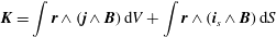 $$\begin{eqnarray}\displaystyle \boldsymbol{K}=\int \boldsymbol{r}\wedge (\boldsymbol{j}\wedge \boldsymbol{B})\,\text{d}V+\int \boldsymbol{r}\wedge (\boldsymbol{i}_{s}\wedge \boldsymbol{B})\,\text{d}S & & \displaystyle\end{eqnarray}$$
can be computed. Beskin et al. (Reference Beskin, Gurevich and Istomin1993) asserted that for an orthogonal rotator with
 $\unicode[STIX]{x1D712}=90^{\circ }$
, the toroidal magnetic field component is much less than the poloidal one in such a way that
$\unicode[STIX]{x1D712}=90^{\circ }$
, the toroidal magnetic field component is much less than the poloidal one in such a way that
 $$\begin{eqnarray}\displaystyle \left.B_{\unicode[STIX]{x1D711}}\right|_{r_{L}}\approx \sqrt{\frac{R}{r_{L}}}\left.B_{p}\right|_{r_{L}} & & \displaystyle\end{eqnarray}$$
with thus a spin-down rate much smaller for the orthogonal case compared to the aligned case. However, simulations show that the spin-down is the same in both geometries within a factor two, therefore the current in the magnetosphere must be much higher in the orthogonal rotator to compensate for the decrease in Poynting flux. Beskin & Zheltoukhov (Reference Beskin and Zheltoukhov2014) also claimed that in such a magnetosphere
 $\unicode[STIX]{x1D6FA}(t)\sin \unicode[STIX]{x1D712}(t)=\text{cst}$
. The obliquity has a tendency to increase with time on a time scale
$\unicode[STIX]{x1D6FA}(t)\sin \unicode[STIX]{x1D712}(t)=\text{cst}$
. The obliquity has a tendency to increase with time on a time scale
 $\unicode[STIX]{x1D70F}_{\unicode[STIX]{x1D712}}\approx P/2{\dot{P}}$
, conflicting with the vacuum expectations.
$\unicode[STIX]{x1D70F}_{\unicode[STIX]{x1D712}}\approx P/2{\dot{P}}$
, conflicting with the vacuum expectations.
3.6 Quantitative magnetospheric structure
In some special cases, exact analytical solutions have been found with and without longitudinal currents. They are summarized in chapter two of Beskin (Reference Beskin2010). They represent interesting models to understand and quantify the back reaction of the current onto the magnetosphere. Let us briefly note some general comments. In the force-free case, solutions only exist in regions where
 $E<cB$
otherwise the force-free condition would be violated. Moreover, if
$E<cB$
otherwise the force-free condition would be violated. Moreover, if
 $j_{\Vert }=0$
, it can be shown that the magnetic field must be perpendicular to the light cylinder and therefore no Poynting flux crosses this surface. So we get the important result that no spin-down is allowed in the force-free regime if there is no longitudinal current. In addition, the poloidal current tends to concentrate magnetic field lines towards the equator. If
$j_{\Vert }=0$
, it can be shown that the magnetic field must be perpendicular to the light cylinder and therefore no Poynting flux crosses this surface. So we get the important result that no spin-down is allowed in the force-free regime if there is no longitudinal current. In addition, the poloidal current tends to concentrate magnetic field lines towards the equator. If
 $j_{\Vert }\gg j_{cor}$
then the light surface is rejected to infinity, otherwise, with
$j_{\Vert }\gg j_{cor}$
then the light surface is rejected to infinity, otherwise, with
 $j_{\Vert }\ll j_{cor}$
there exists a natural boundary on the force-free region given by
$j_{\Vert }\ll j_{cor}$
there exists a natural boundary on the force-free region given by
 $E=cB$
and close to the light cylinder. Petrova (Reference Petrova2013) gave recently also a new exact analytical solution for the axisymmetric magnetosphere. Special focus along the magnetic axis was also performed by Petrova (Reference Petrova2012).
$E=cB$
and close to the light cylinder. Petrova (Reference Petrova2013) gave recently also a new exact analytical solution for the axisymmetric magnetosphere. Special focus along the magnetic axis was also performed by Petrova (Reference Petrova2012).
Let us stress that the space charge available in a pulsar can drastically deviate from the charge necessary to screen the electric field, several processes are list below
-
(i) Particle inertia (Michel Reference Michel1974a ).
-
(ii) Curvature of field lines (Arons Reference Arons1981).
-
(iii) General-relativistic effect (Beskin Reference Beskin1990; Muslimov & Tsygan Reference Muslimov and Tsygan1992).
-
(iv) Inefficient particle extraction (Ruderman & Sutherland Reference Ruderman and Sutherland1975).
4 Other effects on the magnetosphere
So far, most pulsar magnetosphere investigations have tried to solve the Maxwell equations in a flat space–time assuming the lowest-order magnetic field structure: a rotating dipole. There are several caveats to these assumptions. First, it is clear that close to the neutron star, especially at the polar caps, strong gravitational effects would distort the electromagnetic fields due to space–time curvature and frame dragging. Second, it is not excluded that higher multipolar components exist in the magnetosphere, producing polar cap shapes very different from the dipole. These could in principle be observed in the pulsed radio emission through the pulse profile and phase-resolved polarization signature and maybe also in high-energy light curves. Third, with young pulsars, and even more so for magnetars, the magnetic field strength approaches or exceeds the critical value
 $B_{qed}$
. Quantum electrodynamic corrections should then be applied to the magnetosphere according to, for instance, the effective Euler–Heisenberg Lagrangian (Heisenberg & Euler Reference Heisenberg and Euler1936). A direct indisputable consequence of quantum electrodynamics (QED) is pair creation in the vicinity of the surface, a crucial effect to fill the magnetosphere with charged particles. We briefly comment on these issues in this section.
$B_{qed}$
. Quantum electrodynamic corrections should then be applied to the magnetosphere according to, for instance, the effective Euler–Heisenberg Lagrangian (Heisenberg & Euler Reference Heisenberg and Euler1936). A direct indisputable consequence of quantum electrodynamics (QED) is pair creation in the vicinity of the surface, a crucial effect to fill the magnetosphere with charged particles. We briefly comment on these issues in this section.
4.1 General relativity
Soon after the discovery of the first pulsar, there was no doubt that it harboured a strongly magnetised and rotating neutron star. The electromagnetic field generated in vacuum for such a rotator was known since the work by Deutsch (Reference Deutsch1955), although applied to non-compact stars. But we know that neutron stars are very compact because of a compactness parameter given by (2.5), i.e. they almost resemble black holes.
Few, but exact, analytical solutions exist for the structure of the magnetic field in strong gravitational fields. For instance, expressions for a static magnetic dipole field were given by Ginzburg & Ozernoy (Reference Ginzburg and Ozernoy1964) and by Petterson (Reference Petterson1974). Multipoles have been given by Anderson & Cohen (Reference Anderson and Cohen1970). As for flat space–time (Michel Reference Michel1973b ), useful expressions exist for the force-free monopole in the Schwarzschild metric, see Lyutikov (Reference Lyutikov2011), although frame dragging was discarded.
Cohen & Toton (Reference Cohen and Toton1974) showed in the case of an aligned rotator that the electric field induced by the dragging of inertial frames can be as important as the field induced by the rotation itself. These results were generalized for an oblique rotator a few years later by Cohen & Kearney (Reference Cohen and Kearney1980) thanks to a formalism developed previously by Cohen & Kegeles (Reference Cohen and Kegeles1974a
,Reference Cohen and Kegeles
b
, Reference Cohen and Kegeles1975). This demonstrated clearly that a quantitative analysis of the acceleration processes and radiation in the vicinity of the neutron star can only be done by a treatment of the Maxwell equations in the presence of a strong gravitational field. In this way Pfarr (Reference Pfarr1976) looked for an approximate solution to the Maxwell equations in curved space–time, Schwarzschild or Kerr, through a linearized approach using the Newman–Penrose formalism (Newman & Penrose Reference Newman and Penrose1962). He computed the emission of electromagnetic waves in vacuum for a rotating dipole in general relativity with an expression for the Poynting flux
 ${\dot{E}}$
depending on
${\dot{E}}$
depending on
 $R/r_{L}$
. He found the following expression for a Schwarzschild metric
$R/r_{L}$
. He found the following expression for a Schwarzschild metric
 $$\begin{eqnarray}\displaystyle {\dot{E}}_{gr}\approx \frac{{\dot{E}}_{\bot }}{1+(R/r_{L})^{2}}\left(1-\frac{3}{2}\frac{R_{s}}{R}+\frac{R_{s}}{R}\times \text{correction in}\left(\frac{R}{r_{L}}\right)\right) & & \displaystyle\end{eqnarray}$$
thus close to the Deutsch,
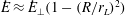 ${\dot{E}}\approx {\dot{E}}_{\bot }(1-(R/r_{L})^{2})$
expectation for
${\dot{E}}\approx {\dot{E}}_{\bot }(1-(R/r_{L})^{2})$
expectation for
 $R_{s}=0$
.
$R_{s}=0$
.
 ${\dot{E}}_{gr}$
is the general-relativistic spin-down luminosity and
${\dot{E}}_{gr}$
is the general-relativistic spin-down luminosity and
 ${\dot{E}}_{\bot }$
the flat space–time spin-down luminosity. Muslimov & Tsygan (Reference Muslimov and Tsygan1992) investigated the influence of space–time curvature and frame dragging of inertial frames on the electric field at the polar caps of a pulsar. Sengupta (Reference Sengupta1995) studied in detail the electric field in the Schwarzschild metric for an aligned rotator in vacuum and plunged in a plasma. The result is an important increase in the electric field at the surface of the star, implying a larger charge density and therefore an acceleration of charges which is more efficient, with possible consequences for the high-energy emission of pulsars (Gonthier & Harding Reference Gonthier and Harding1994). The aligned rotator was revived by Konno & Kojima (Reference Konno and Kojima2000) for investigations of particle acceleration in vacuum. Rezzolla, Ahmedov & Miller (Reference Rezzolla, Ahmedov and Miller2001), Zanotti & Rezzolla (Reference Zanotti and Rezzolla2002), Rezzolla & Ahmedov (Reference Rezzolla and Ahmedov2004) and Pétri (Reference Pétri2013a
) computed the effects of general relativity on the electromagnetic field around a slowly rotating neutron star. Rezzolla & Ahmedov (Reference Rezzolla and Ahmedov2016) built on their previous results and computed the damping of oscillations via Joule heating and Ohmic dissipation. Muslimov & Harding (Reference Muslimov and Harding1997) and Sakai & Shibata (Reference Sakai and Shibata2003) were concerned about particle acceleration around polar caps in curved space–time. Kojima, Matsunaga & Okita (Reference Kojima, Matsunaga and Okita2004) looked for approximate analytical solutions to the oblique rotator problem in vacuum in general relativity. They furnished an approximate numerical solution, expanded to first order. A treatment of the magnetosphere with help of the Grad–Shafranov equation has been exploited by Kim et al. (Reference Kim, Lee, Lee and Lee2005). Morozova, Ahmedov & Zanotti (Reference Morozova, Ahmedov and Zanotti2010) studied the influence of neutron star oscillations in general relativity on the corotation density in the magnetosphere for a aligned rotator. Pétri (Reference Pétri2016a
) made an extensive study of force-free pulsar magnetospheres in general relativity. General relativity seems to play a decisive role for efficient pair creation at the surface (Philippov et al.
Reference Philippov, Cerutti, Tchekhovskoy and Spitkovsky2015a
; Belyaev & Parfrey Reference Belyaev and Parfrey2016).
${\dot{E}}_{\bot }$
the flat space–time spin-down luminosity. Muslimov & Tsygan (Reference Muslimov and Tsygan1992) investigated the influence of space–time curvature and frame dragging of inertial frames on the electric field at the polar caps of a pulsar. Sengupta (Reference Sengupta1995) studied in detail the electric field in the Schwarzschild metric for an aligned rotator in vacuum and plunged in a plasma. The result is an important increase in the electric field at the surface of the star, implying a larger charge density and therefore an acceleration of charges which is more efficient, with possible consequences for the high-energy emission of pulsars (Gonthier & Harding Reference Gonthier and Harding1994). The aligned rotator was revived by Konno & Kojima (Reference Konno and Kojima2000) for investigations of particle acceleration in vacuum. Rezzolla, Ahmedov & Miller (Reference Rezzolla, Ahmedov and Miller2001), Zanotti & Rezzolla (Reference Zanotti and Rezzolla2002), Rezzolla & Ahmedov (Reference Rezzolla and Ahmedov2004) and Pétri (Reference Pétri2013a
) computed the effects of general relativity on the electromagnetic field around a slowly rotating neutron star. Rezzolla & Ahmedov (Reference Rezzolla and Ahmedov2016) built on their previous results and computed the damping of oscillations via Joule heating and Ohmic dissipation. Muslimov & Harding (Reference Muslimov and Harding1997) and Sakai & Shibata (Reference Sakai and Shibata2003) were concerned about particle acceleration around polar caps in curved space–time. Kojima, Matsunaga & Okita (Reference Kojima, Matsunaga and Okita2004) looked for approximate analytical solutions to the oblique rotator problem in vacuum in general relativity. They furnished an approximate numerical solution, expanded to first order. A treatment of the magnetosphere with help of the Grad–Shafranov equation has been exploited by Kim et al. (Reference Kim, Lee, Lee and Lee2005). Morozova, Ahmedov & Zanotti (Reference Morozova, Ahmedov and Zanotti2010) studied the influence of neutron star oscillations in general relativity on the corotation density in the magnetosphere for a aligned rotator. Pétri (Reference Pétri2016a
) made an extensive study of force-free pulsar magnetospheres in general relativity. General relativity seems to play a decisive role for efficient pair creation at the surface (Philippov et al.
Reference Philippov, Cerutti, Tchekhovskoy and Spitkovsky2015a
; Belyaev & Parfrey Reference Belyaev and Parfrey2016).
Note that black hole magnetospheres can be treated similarly to neutron stars, except for the presence of an event horizon for the former. The problem of this horizon is solved by a change of spatio-temporal coordinates to the Kerr–Schild metric for instance. This coordinate transform permitted the numerical study of the monopolar solution of the black hole magnetosphere presented by Komissarov (Reference Komissarov2004). He used a 3+1 formulation of electrodynamics in general relativity. It is useful for pulsars and black holes, and nicely summarized by Komissarov (Reference Komissarov2011). Space–time is decomposed into an ‘absolute’ time and a three-dimensional ‘curved space’ to come back to more traditional hyperbolic systems for the Maxwell equations in flat space–time. Yu (Reference Yu2007) used the same formalism for the force-free regime for the magnetosphere of an axisymmetric black hole. Morozova, Ahmedov & Kagramanova (Reference Morozova, Ahmedov and Kagramanova2008) extended the general-relativistic field to a special space–time geometry called NUT space (Newman–Unti–Tamburino).
4.2 Multipoles
Most pulsar emission models assume a dipolar magnetic field anchored right at the centre of the star. This hypothesis is certainly correct far from the star, around the light cylinder and beyond, since the high-order multipoles
 $\ell$
decrease with radius faster than low-order ones, like
$\ell$
decrease with radius faster than low-order ones, like
 $r^{-(\ell +1)}$
. But nothing forbids the existence of significant multipolar components in the vicinity of the star. Multipoles are easily induced by a rotating decentred dipole. The consequences of an off-centred dipole on neutron star proper motion and torque was the main topic in Roberts (Reference Roberts1979). Following the same line, Cohen & Rosenblum (Reference Cohen and Rosenblum1972) showed how to compute force-free multipole components close to the surface with an extension to include general-relativistic effects (Cohen & Rosenblum Reference Cohen and Rosenblum1973). Roberts (Reference Roberts1979) developed a general formalism for computing the multipolar electromagnetic moments of a neutron star, therewith explaining the high velocity of pulsars through asymmetric radiation when the progenitor exploded, an early idea by Harrison & Tademaru (Reference Harrison and Tademaru1975). Krolik (Reference Krolik1991) studied the influence of multipoles on the estimate of millisecond pulsars magnetic fields and rotational braking via their braking indices. Asseo & Khechinashvili (Reference Asseo and Khechinashvili2002) discussed the role of multipoles on the radiation processes and pair creation in the magnetosphere and Kantor & Tsygan (Reference Kantor and Tsygan2003) evoked the influence on the current emanating from the polar caps. Barsukov & Tsygan (Reference Barsukov and Tsygan2010) showed an alteration of radiative dipolar magnetic losses because of the presence of multipolar components. Obviously, the polar caps geometry is strongly tributary to multipolar components (Zhang & Qiao Reference Zhang and Qiao1996) with important consequences on radio emission but also on pair creation in such fields (Jones Reference Jones1980; Harding & Muslimov Reference Harding and Muslimov2011). Magnetic multipoles also have an impact on accretion processes to spin-up neutron stars to millisecond periods. The derived spin-up line in the
$r^{-(\ell +1)}$
. But nothing forbids the existence of significant multipolar components in the vicinity of the star. Multipoles are easily induced by a rotating decentred dipole. The consequences of an off-centred dipole on neutron star proper motion and torque was the main topic in Roberts (Reference Roberts1979). Following the same line, Cohen & Rosenblum (Reference Cohen and Rosenblum1972) showed how to compute force-free multipole components close to the surface with an extension to include general-relativistic effects (Cohen & Rosenblum Reference Cohen and Rosenblum1973). Roberts (Reference Roberts1979) developed a general formalism for computing the multipolar electromagnetic moments of a neutron star, therewith explaining the high velocity of pulsars through asymmetric radiation when the progenitor exploded, an early idea by Harrison & Tademaru (Reference Harrison and Tademaru1975). Krolik (Reference Krolik1991) studied the influence of multipoles on the estimate of millisecond pulsars magnetic fields and rotational braking via their braking indices. Asseo & Khechinashvili (Reference Asseo and Khechinashvili2002) discussed the role of multipoles on the radiation processes and pair creation in the magnetosphere and Kantor & Tsygan (Reference Kantor and Tsygan2003) evoked the influence on the current emanating from the polar caps. Barsukov & Tsygan (Reference Barsukov and Tsygan2010) showed an alteration of radiative dipolar magnetic losses because of the presence of multipolar components. Obviously, the polar caps geometry is strongly tributary to multipolar components (Zhang & Qiao Reference Zhang and Qiao1996) with important consequences on radio emission but also on pair creation in such fields (Jones Reference Jones1980; Harding & Muslimov Reference Harding and Muslimov2011). Magnetic multipoles also have an impact on accretion processes to spin-up neutron stars to millisecond periods. The derived spin-up line in the
 $P{-}{\dot{P}}$
diagram could constrain multipole moments (Arons Reference Arons1993).
$P{-}{\dot{P}}$
diagram could constrain multipole moments (Arons Reference Arons1993).
Very recently, Bonazzola, Mottez & Heyvaerts (Reference Bonazzola, Mottez and Heyvaerts2015) and Pétri (Reference Pétri2015d ) gave exact analytical expressions for any multipolar electromagnetic field in vacuum. It represents a generalisation of the Deutsch field solutions in terms of spherical Hankel functions. Arzamasskiy, Philippov & Tchekhovskoy (Reference Arzamasskiy, Philippov and Tchekhovskoy2015) investigated the influence of an aspherical shape of the neutron star on its rotational motion and showed that even a very small ellipticity leads to a precession of period compatible with timing residuals. They took into account the presence of a plasma in the magnetosphere. Aspherical shapes can also give rise to multipolar fields.
Observational support for the presence of multipoles are given already for main sequence stars. Stift (Reference Stift1974) looked at decentred dipole in stars with a displacement along the magnetic axis. Off-centred dipole is already present in AP stars to solve the asymmetry problem between the north and south hemisphere (Landstreet Reference Landstreet1970). An off-centred dipole is also the preferred way to explain the Zeeman line profile, as explained in Borra (Reference Borra1974). In the context of high-energy processes around compact objects, the radio emission of PSR J2144-3933 is explained with a novel model of pair creation in the magnetosphere (Zhang, Harding & Muslimov Reference Zhang, Harding and Muslimov2000) or simply by the presence of intense multipolar components of the surface magnetic field in all radio pulsars (Gil & Mitra Reference Gil and Mitra2001; Gil, Melikidze & Mitra Reference Gil, Melikidze and Mitra2002).
Magnetospheric topologies that deviate slightly or significantly from a pure dipole represent attractive explanations for many electromagnetic phenomena occurring in the neighbourhood of neutron stars. Twisted magnetospheres are especially investigated to understand flares in magnetars (Beloborodov Reference Beloborodov2009; Viganò, Pons & Miralles Reference Viganò, Pons and Miralles2011; Pili, Bucciantini & Del Zanna Reference Pili, Bucciantini and Del Zanna2015; Akgün et al. Reference Akgün, Miralles, Pons and Cerdá-Durán2016) and also to account for the mode switching and related spin-down changes in intermittent pulsars (Huang, Yu & Tong Reference Huang, Yu and Tong2016).
4.3 Quantum electrodynamics
The ultra-strong magnetic field inferred from the global energetics of pulsars approaches, or even exceeds, the quantum critical value of
 $B_{qed}$
. Quantum electrodynamics is therefore required to correctly describe the physics in such fields. Pair creation is the most important effect, feeding the neutron star surroundings with fresh and ultra-relativistic electron/positron pairs. But this process works on a local scale useful to understand microphysics phenomena. The question arises of the impact of quantum electrodynamics on the global energetic evolution of pulsar spin-down luminosity. This topic was touched on by several authors and it seems that, even for magnetar field strengths, the corrections from QED remain weak (Heyl & Hernquist Reference Heyl and Hernquist1997). QED effects can be combined with general relativity in the 3+1 formalism, as shown by Pétri (Reference Pétri2015a
). Applications for a static oblique dipole are given by Pétri (Reference Pétri2016b
). Recent numerical simulations of a general-relativistic quantum electrodynamics (GRQED) and general-relativistic force-free quantum electrodynamics (GRFFQED) rotating dipole confirm the absence of significant corrections to the spin-down (Petri Reference Petri2016).
$B_{qed}$
. Quantum electrodynamics is therefore required to correctly describe the physics in such fields. Pair creation is the most important effect, feeding the neutron star surroundings with fresh and ultra-relativistic electron/positron pairs. But this process works on a local scale useful to understand microphysics phenomena. The question arises of the impact of quantum electrodynamics on the global energetic evolution of pulsar spin-down luminosity. This topic was touched on by several authors and it seems that, even for magnetar field strengths, the corrections from QED remain weak (Heyl & Hernquist Reference Heyl and Hernquist1997). QED effects can be combined with general relativity in the 3+1 formalism, as shown by Pétri (Reference Pétri2015a
). Applications for a static oblique dipole are given by Pétri (Reference Pétri2016b
). Recent numerical simulations of a general-relativistic quantum electrodynamics (GRQED) and general-relativistic force-free quantum electrodynamics (GRFFQED) rotating dipole confirm the absence of significant corrections to the spin-down (Petri Reference Petri2016).
On a smaller scale, the strong magnetic field anchored into the neutron star induces vacuum birefringence and modifies the way electromagnetic waves propagate in vacuum (Ho & Lai Reference Ho and Lai2001, Reference Ho and Lai2003; Lai & Ho Reference Lai and Ho2003; Gapochka et al.
Reference Gapochka, Denisov, Denisova, Kalenova and Korolev2015). Especially, two normal modes that have mutual orthogonal polarisation travel at different speed in the magnetosphere (Harding & Lai Reference Harding and Lai2006; Denisov, Sokolov & Vasili’ev Reference Denisov, Sokolov and Vasili’ev2014). Abishev et al. (Reference Abishev, Aimuratov, Aldabergenov, Beissen, Bakytzhan and Takibayeva2016) estimated that the delay observed by a detector at Earth would be of the order
 $\unicode[STIX]{x0394}t\approx 10^{-8}$
s, but unfortunately too weak for current instrumentation. Denisov & Svertilov (Reference Denisov and Svertilov2005) showed that gravity can be combined with QED to study light propagation in a realistic neutron star environment. See also Freytsis & Gralla (Reference Freytsis and Gralla2016) for a broader discussion about force-free theories including a general Lagrangian not necessarily issued from quantum electrodynamics. Bending of a light ray due to QED effects was also mentioned by several groups including Shabad & Usov (Reference Shabad and Usov1982, Reference Shabad and Usov1984) and Denisov & Svertilov (Reference Denisov and Svertilov2003). Nonlinear electrodynamics induces a supplementary redshift compared to gravitation, rendering the compactness
$\unicode[STIX]{x0394}t\approx 10^{-8}$
s, but unfortunately too weak for current instrumentation. Denisov & Svertilov (Reference Denisov and Svertilov2005) showed that gravity can be combined with QED to study light propagation in a realistic neutron star environment. See also Freytsis & Gralla (Reference Freytsis and Gralla2016) for a broader discussion about force-free theories including a general Lagrangian not necessarily issued from quantum electrodynamics. Bending of a light ray due to QED effects was also mentioned by several groups including Shabad & Usov (Reference Shabad and Usov1982, Reference Shabad and Usov1984) and Denisov & Svertilov (Reference Denisov and Svertilov2003). Nonlinear electrodynamics induces a supplementary redshift compared to gravitation, rendering the compactness
 $M/R$
difficult to estimate (Mosquera Cuesta & Salim Reference Mosquera Cuesta and Salim2004).
$M/R$
difficult to estimate (Mosquera Cuesta & Salim Reference Mosquera Cuesta and Salim2004).
4.4 Pair creation
Along field lines with strong intensity, electrons and positrons copiously radiate synchrotron photons on a very short cooling time scale of approximately
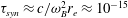 $\unicode[STIX]{x1D70F}_{syn}\approx c/\unicode[STIX]{x1D714}_{B}^{2}r_{e}\approx 10^{-15}$
s, thus much smaller than the pulsar period. To a good approximation, we can say that in vacuum, leptons reach quasi-instantaneously ultra-relativistic speed as soon as they are created around the poles. Besides synchrotron emission, curvature radiation furnishes also numerous photons disintegrating in this magnetic field via the channel
$\unicode[STIX]{x1D70F}_{syn}\approx c/\unicode[STIX]{x1D714}_{B}^{2}r_{e}\approx 10^{-15}$
s, thus much smaller than the pulsar period. To a good approximation, we can say that in vacuum, leptons reach quasi-instantaneously ultra-relativistic speed as soon as they are created around the poles. Besides synchrotron emission, curvature radiation furnishes also numerous photons disintegrating in this magnetic field via the channel
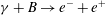 $$\begin{eqnarray}\displaystyle \unicode[STIX]{x1D6FE}+B\rightarrow e^{-}+e^{+} & & \displaystyle\end{eqnarray}$$
according to a probability per unit length given by Erber (Reference Erber1966) from which we deduce a mean free path of
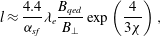 $$\begin{eqnarray}\displaystyle l\approx \frac{4.4}{\unicode[STIX]{x1D6FC}_{sf}}\unicode[STIX]{x1D706}_{e}\frac{B_{qed}}{B_{\bot }}\exp \left(\frac{4}{3\unicode[STIX]{x1D712}}\right), & & \displaystyle\end{eqnarray}$$
with
 $$\begin{eqnarray}\displaystyle \unicode[STIX]{x1D712}=\frac{\unicode[STIX]{x1D716}_{\unicode[STIX]{x1D6FE}}}{2m_{e}c^{2}}\frac{B_{\bot }}{B_{qed}} & & \displaystyle\end{eqnarray}$$
valid in the limit
 $\unicode[STIX]{x1D712}\ll 1$
. Curvature emission is not the only source of electron–positron pairs in the polar caps. Indeed, it was realized in the middle of the 1990s (Kundt & Schaaf Reference Kundt and Schaaf1993; Sturner, Dermer & Michel Reference Sturner, Dermer and Michel1995; Luo Reference Luo1996; Zhang & Qiao Reference Zhang and Qiao1996) that inverse Compton scattering of the thermal radiation from the star surface provides gamma rays decaying in pairs at energies of the primary electrons much smaller than a few TeV required by the classical models. The process has been extensively studied in the literature.
$\unicode[STIX]{x1D712}\ll 1$
. Curvature emission is not the only source of electron–positron pairs in the polar caps. Indeed, it was realized in the middle of the 1990s (Kundt & Schaaf Reference Kundt and Schaaf1993; Sturner, Dermer & Michel Reference Sturner, Dermer and Michel1995; Luo Reference Luo1996; Zhang & Qiao Reference Zhang and Qiao1996) that inverse Compton scattering of the thermal radiation from the star surface provides gamma rays decaying in pairs at energies of the primary electrons much smaller than a few TeV required by the classical models. The process has been extensively studied in the literature.
Secondary plasma generations are created following two different models
-
(i) For Ruderman & Sutherland (Reference Ruderman and Sutherland1975), particles cannot freely escape from the surface, thus producing a charge density different from the corotation
$\unicode[STIX]{x1D70C}\neq \unicode[STIX]{x1D70C}_{cor}$
. The longitudinal electric field builds up approximatively like (4.5)in the corotating frame where
$$\begin{eqnarray}\displaystyle \frac{\text{d}E_{\Vert }}{\text{d}h}=\frac{\unicode[STIX]{x1D70C}-\unicode[STIX]{x1D70C}_{cor}}{\unicode[STIX]{x1D700}_{0}} & & \displaystyle\end{eqnarray}$$
$E_{\Vert }$
is the parallel electric field and
$h$
the altitude measured from the surface. Particles do not circulate freely and the longitudinal electric field becomes, with the Ruderman–Sutherland field
$E_{RS}$
and
$H$
the size of the gap, (4.6)
$$\begin{eqnarray}\displaystyle E_{\Vert }=E_{RS}\frac{H-h}{H}. & & \displaystyle\end{eqnarray}$$
-
(ii) On the contrary, for Fawley, Arons & Scharlemann (Reference Fawley, Arons and Scharlemann1977), Scharlemann, Arons & Fawley (Reference Scharlemann, Arons and Fawley1978), Arons & Scharlemann (Reference Arons and Scharlemann1979), particles circulate freely leading to the boundary conditions on the gaps as
$E_{\Vert }(h=0)=E_{\Vert }(H=0)=0$
and corotation charge density
$\unicode[STIX]{x1D70C}=\unicode[STIX]{x1D70C}_{cor}$
.


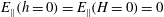

Primary particles are believed to reach
 $E\approx 10^{7}$
MeV whereas secondary pairs only reach
$E\approx 10^{7}$
MeV whereas secondary pairs only reach
 $E\approx 10^{2}{-}10^{4}$
MeV with a particle distribution function close to
$E\approx 10^{2}{-}10^{4}$
MeV with a particle distribution function close to
 $N(E)\propto E^{-2}$
and a multiplicity
$N(E)\propto E^{-2}$
and a multiplicity
 $\unicode[STIX]{x1D705}\approx 10^{3}{-}10^{4}$
(Beskin Reference Beskin2010). The global picture of the polar outflow is a primary beam of charged particles with high Lorentz factor
$\unicode[STIX]{x1D705}\approx 10^{3}{-}10^{4}$
(Beskin Reference Beskin2010). The global picture of the polar outflow is a primary beam of charged particles with high Lorentz factor
 $\unicode[STIX]{x1D6FE}_{b}\approx 10^{7}$
producing cascades of
$\unicode[STIX]{x1D6FE}_{b}\approx 10^{7}$
producing cascades of
 $e^{\pm }$
pairs at a multiplicity
$e^{\pm }$
pairs at a multiplicity
 $\unicode[STIX]{x1D705}\approx 10^{2}{-}10^{4}$
with lower Lorentz factor
$\unicode[STIX]{x1D705}\approx 10^{2}{-}10^{4}$
with lower Lorentz factor
 $\unicode[STIX]{x1D6FE}_{s}\approx 10^{2}{-}10^{3}$
(Arendt & Eilek Reference Arendt and Eilek2002). These pairs are produced by resonant or non-resonant inverse Compton scattering, depending on the neutron star surface temperature and curvature radiation (Hibschman & Arons Reference Hibschman and Arons2001a
,Reference Hibschman and Arons
b
). Radiation emanating from this pair creation process was investigated by Luo & Ji (Reference Luo and Ji2015) using the Vlasov–Maxwell equations.
$\unicode[STIX]{x1D6FE}_{s}\approx 10^{2}{-}10^{3}$
(Arendt & Eilek Reference Arendt and Eilek2002). These pairs are produced by resonant or non-resonant inverse Compton scattering, depending on the neutron star surface temperature and curvature radiation (Hibschman & Arons Reference Hibschman and Arons2001a
,Reference Hibschman and Arons
b
). Radiation emanating from this pair creation process was investigated by Luo & Ji (Reference Luo and Ji2015) using the Vlasov–Maxwell equations.
4.5 Magnetic reconnection
Removing the ideal MHD or force-free regime by adding resistivity or other dissipative effects leads to violation of the flux freezing condition. In addition, a rearrangement of the magnetic topology is expected via magnetic reconnection. This process can drastically perturb the initial magnetic configuration and induces non-stationary states in the magnetosphere. Already in the early 1970s Scargle & Pacini (Reference Scargle and Pacini1971) claimed that an explosive inflation of the magnetospheric plasma could explain the observed glitch phenomena in the Crab pulsar. Tearing instabilities were very popular in the 1980s and applied for an electron–positron plasma in pulsar magnetospheres by Shukla, Yu & Pavlenko (Reference Shukla, Yu and Pavlenko1987) as an onset for magnetic reconnection events. Contopoulos (Reference Contopoulos2005, Reference Contopoulos2007b
) invoked reconnection in the vicinity of the light cylinder with possible implications for the braking index (Contopoulos Reference Contopoulos2007a
). The slowing down of the neutron star inflates the size of the light cylinder. Open field lines in the vicinity of the separatrix must reconnect and close, switching to the closed and corotating part of the plasma. This can be seen as a shift in the Y-point. According to Ardavan (Reference Ardavan1976b
) the force-free condition, or more generally the ideal MHD regime, is violated whenever the criterion
 $(Lc/\unicode[STIX]{x1D714}_{p})^{2}\ll 1$
is no more satisfied where
$(Lc/\unicode[STIX]{x1D714}_{p})^{2}\ll 1$
is no more satisfied where
 $L$
is a typical gradient scale of macroscopic quantities and
$L$
is a typical gradient scale of macroscopic quantities and
 $\unicode[STIX]{x1D714}_{p}$
the plasma proper frame frequency. Therefore, corotation cannot be maintained outside a critical radius
$\unicode[STIX]{x1D714}_{p}$
the plasma proper frame frequency. Therefore, corotation cannot be maintained outside a critical radius
 $r_{c}<r_{L}$
inside the light cylinder and depending on local plasma conditions. The exact expression for the particle Lorentz factor near the light cylinder found by Ardavan (Reference Ardavan1976b
) has been criticized by Burman (Reference Burman1977b
). The former forgot to include inertial drift in his integral of motion (Burman Reference Burman1980a
,Reference Burman
b
). Recently, Bogovalov (Reference Bogovalov2014) showed that bulk flow acceleration to a very high Lorentz factor such as
$r_{c}<r_{L}$
inside the light cylinder and depending on local plasma conditions. The exact expression for the particle Lorentz factor near the light cylinder found by Ardavan (Reference Ardavan1976b
) has been criticized by Burman (Reference Burman1977b
). The former forgot to include inertial drift in his integral of motion (Burman Reference Burman1980a
,Reference Burman
b
). Recently, Bogovalov (Reference Bogovalov2014) showed that bulk flow acceleration to a very high Lorentz factor such as
 $\unicode[STIX]{x1D6E4}\approx (1-r^{2}/r_{L}^{2})^{-1}$
can occur close to the light cylinder provided magnetic field lines are swept forward in the hope of explaining the very high-energy pulsed emission of the Crab. An alternative production of these very high energy (VHE) would be by parallel electric field acceleration in the outer gap close to the light cylinder (Bednarek Reference Bednarek2012) but this mechanism has been criticized by Hirotani (Reference Hirotani2014).
$\unicode[STIX]{x1D6E4}\approx (1-r^{2}/r_{L}^{2})^{-1}$
can occur close to the light cylinder provided magnetic field lines are swept forward in the hope of explaining the very high-energy pulsed emission of the Crab. An alternative production of these very high energy (VHE) would be by parallel electric field acceleration in the outer gap close to the light cylinder (Bednarek Reference Bednarek2012) but this mechanism has been criticized by Hirotani (Reference Hirotani2014).
4.6 Magnetospheric oscillations
Already in 1965, Cameron (Reference Cameron1965) suggested that neutron star oscillations could generate electromagnetic activity in a neutron star magnetosphere and account for the X-ray observations in the Crab nebula known at that time. Investigations of oscillations above the polar caps have been conducted by many authors to generate, for instance, radio wave (Rylov Reference Rylov1978), two-stream instabilities maintaining oscillations and converted into radiation (Lyubarskij Reference Lyubarskij1993) or to explain the drifting subpulses (Clemens & Rosen Reference Clemens and Rosen2004). Morozova, Ahmedov & Zanotti (Reference Morozova, Ahmedov and Zanotti2014) adopted a space-charge limited flow point of view in general relativity to interpret the same phenomenon. Oscillations could trigger magnetospheric activity and relate to the radio emission of normal pulsars and magnetars (Lin, Xu & Zhang Reference Lin, Xu and Zhang2015). Stellar oscillations impact on the maximum Lorentz factor of particles accelerated in the polar cap (Zanotti, Morozova & Ahmedov Reference Zanotti, Morozova and Ahmedov2012). Oscillations in magnetars are able to shift the radio emission generation threshold to less restrictive regions in the
 $P{-}{\dot{P}}$
diagram (Morozova, Ahmedov & Zanotti Reference Morozova, Ahmedov and Zanotti2012). Oscillations are relevant for magnetar quasi-periodic oscillations (Abdikamalov, Ahmedov & Miller Reference Abdikamalov, Ahmedov and Miller2009). Kojima & Kato (Reference Kojima and Kato2014) included some resistivity prescription and perturbed the magnetosphere through torsional shear oscillations hoping to explain X-ray and gamma-ray flares in magnetars. The presence of a plasma oscillating in the magnetosphere modifies the energy loss depending on the oscillation frequency compared to vacuum (Timokhin, Bisnovatyi-Kogan & Spruit Reference Timokhin, Bisnovatyi-Kogan and Spruit2000).
$P{-}{\dot{P}}$
diagram (Morozova, Ahmedov & Zanotti Reference Morozova, Ahmedov and Zanotti2012). Oscillations are relevant for magnetar quasi-periodic oscillations (Abdikamalov, Ahmedov & Miller Reference Abdikamalov, Ahmedov and Miller2009). Kojima & Kato (Reference Kojima and Kato2014) included some resistivity prescription and perturbed the magnetosphere through torsional shear oscillations hoping to explain X-ray and gamma-ray flares in magnetars. The presence of a plasma oscillating in the magnetosphere modifies the energy loss depending on the oscillation frequency compared to vacuum (Timokhin, Bisnovatyi-Kogan & Spruit Reference Timokhin, Bisnovatyi-Kogan and Spruit2000).
Usually the matter content of pulsar magnetospheres is assumed to be made of light particles, leptons that do not contribute significantly to the total mass of the pulsar. Nevertheless, several authors considered the effect of a mass loaded magnetosphere, in particular to shift the Y-point inside the light cylinder towards the star (Pustilnik Reference Pustilnik1977). This author also predicted possible episodes of mass ejection related to the glitches. Tsui (Reference Tsui2015) argued that, depending on the plasma and magnetic energy content within the magnetosphere, the pulsar may expel matter sporadically outside the light cylinder.
An important question raised recently by several authors concerns the connection between the neutron star interior to its exterior, i.e. its magnetosphere. Usually, the former community assumes vacuum outside whereas the latter community assumes specific boundary conditions on the surface. Obviously, this approach is neither satisfactory for the first nor for the second community. Thus any realistic solution to the pulsar magnetosphere should join smoothly the interior field to the exterior field. Such rather new investigations including both domains are possible as demonstrated by Ruiz, Paschalidis & Shapiro (Reference Ruiz, Paschalidis and Shapiro2014) who computed the Poynting flux depending on equations of state and compactness. Matching ideal MHD simulations with the force-free schemes was used by Paschalidis & Shapiro (Reference Paschalidis and Shapiro2013) to compute neutron star magnetospheres. Glampedakis, Lander & Andersson (Reference Glampedakis, Lander and Andersson2014) and Pili et al. (Reference Pili, Bucciantini and Del Zanna2015) undertook similar studies. Belvedere, Rueda & Ruffini (Reference Belvedere, Rueda and Ruffini2015) even attempted to compute the full solution inside and outside with realistic equations of state and accounting for all fundamental interactions including general relativity and results from quantum mechanics.
4.7 Non-corotating and highly rotating magnetosphere
In the simplest description of the plasma motion, the electromagnetic field achieves a configuration imposing perfect corotation of the particles at most up to the light cylinder. We stress that this fact is an assumption and not a result of the model. Therefore the question ‘Does pulsar magnetosphere really corotate with the underlying neutron star?’ is meaningful. Such questioning was the subject of several papers, among them Melrose & Yuen (Reference Melrose and Yuen2012, Reference Melrose and Yuen2014, Reference Melrose and Yuen2016) who were preoccupied with the neglect of the inductive electric field in MHD or force-free magnetospheres. Differential rotation of, for instance, the open field lines due to a potential drop above the polar cap changes the value of the electric current density and impacts on the braking index (Timokhin Reference Timokhin2007a ,Reference Timokhin b ).
Dissipation regions where charges are able to cross field lines are compulsory to close the current and transfer angular momentum outside the light cylinder. Fitzpatrick & Mestel (Reference Fitzpatrick and Mestel1988a ,Reference Fitzpatrick and Mestel b ) looked for such solutions.
The Deutsch (Reference Deutsch1955) electromagnetic field expressions, although being an exact analytical solution to the Maxwell equations, fails to give an accurate picture of relativistically rotating neutron stars when
 $R/r_{L}\rightarrow 1$
because it assumes non-relativistic rotation. Belinsky & Ruffini (Reference Belinsky and Ruffini1992), Belinsky et al. (Reference Belinsky, de Paolis, Lee and Ruffini1994) gave an answer to this problem and showed an analogy with synchrotron radiation. de Paolis, Ingrosso & Qadir (Reference de Paolis, Ingrosso and Qadir1995) proposed an alternative derivation of this relativistic rotating dipole. The increase in spin-down power is counterbalanced by gravitational effects when the mass of the dipole is added (Herbst, Qadir & Momoniat Reference Herbst, Qadir and Momoniat2013).
$R/r_{L}\rightarrow 1$
because it assumes non-relativistic rotation. Belinsky & Ruffini (Reference Belinsky and Ruffini1992), Belinsky et al. (Reference Belinsky, de Paolis, Lee and Ruffini1994) gave an answer to this problem and showed an analogy with synchrotron radiation. de Paolis, Ingrosso & Qadir (Reference de Paolis, Ingrosso and Qadir1995) proposed an alternative derivation of this relativistic rotating dipole. The increase in spin-down power is counterbalanced by gravitational effects when the mass of the dipole is added (Herbst, Qadir & Momoniat Reference Herbst, Qadir and Momoniat2013).
5 Numerical simulations
Searching for an analytical solution to the problem of the magnetospheric structure is very cumbersome or even impossible in a realistic situation. Another complementary approach allowing deeper and more quantitative insight consists of performing numerical simulations of the temporal evolution of the magnetosphere. We then hope to observe relaxation to a stationary equilibrium state. The level of complexity of these simulations relies on the approximation used to described the behaviour of plasmas interacting with the stellar electromagnetic field, radiative corrections and self-consistent treatment of particle injection through pair formation. Starting with the crudest physical description, known as the force-free approximation, it is useful to investigate neutron star and also black hole magnetospheres on the largest scales, several other plasma regimes have been or should be explored in the future. The so far most extensively studied are
-
(i) Force-free (magnetodynamics): charge and current carriers have no or negligible mass. They respond instantaneously to the external electromagnetic field to furnish the required charge and current densities imposed by the evolution of the fields. The matter stress–energy tensor vanishes. No energy dissipation occurs.
-
(ii) Resistive magnetodynamics: in order to allow for dissipation and transfer of energy from the field to the particles, some resistive terms are added to the force-free current. The resistivity prescription is not unique and loosely constrained. Motion of the plasma is not solved.
-
(iii) MHD: particle inertia is taken into account and the full stress–energy tensor, matter and field, are solved. Simulations are performed in the ideal limit or in the resistive regime.
-
(iv) Multi-fluids: the electron–positron plasma does not strictly follow the MHD system because both particle species have the same mass. The usual MHD ordering according to the masses is therefore impossible. Multi-fluid schemes evolve each species independently, the coupling going through electromagnetic interactions via Lorentz forces. Binary collisions between particles irrespective of their species are treated following Monte Carlo techniques.
-
(v) Fully kinetic treatment: convenient to account for individual particle acceleration towards distribution functions that are out of thermal equilibrium. Needs to solve the full Vlasov–Maxwell equations and thus very expensive computationally.
-
(vi) Radiation reaction limit: particles in pulsar magnetospheres radiate copiously up to the point where any acceleration is compensated by radiation reaction. In this special case, particle motion can be solved analytically to give an expression for the velocity (equal to the speed of light) only in terms of the external electromagnetic field. It represents an interesting alternative to the full Vlasov–Maxwell approach in the strong radiation reaction limit.
Let us pinpoint the merits of all these approximations.
5.1 Force-free electrodynamics (FFE)
Force-free electrodynamics leads to some degeneracy in its physical interpretation. Indeed, under such a hypothesis, two interpretations are plausible
-
(i) The plasma is non-neutral and therefore completely charge separated. This corresponds to a weak density of particles in the magnetosphere with
$(n_{+},n_{-})\approx n_{cor}$
. Complete charge separation has been criticized by Salvati (Reference Salvati1973). -
(ii) Ideal MHD applies. This implies a quasi-neutral plasma therefore a large particle density number in this same magnetosphere with
$n=n_{+}+n_{-}\gg n_{cor}$
with
$n_{+}\approx n_{-}$
but a small difference to allow room for a possible small electric charge density such that
$|n_{+}-n_{-}|\ll n$
.


Which of these views prevail in a realistic magnetosphere? It depends on the injection rate of charged particles, a direct consequence of efficient pair formation in the vacuum gaps, a still unsolved problem. Nevertheless nebulas seem to prefer the second option of a dense plasma, we will explain why in the section about pulsar winds. However, major problems arise from unconstrained global features, namely
-
(i) The total charge of the star and its surrounding magnetosphere remains unconstrained and worse, not necessarily null. However, Jackson (Reference Jackson1976a ,Reference Jackson b ) gave an argument to constrain the electric charge of the star to such a value as to stop leakage towards the nebula, assuming that only electrons leave the star.
-
(ii) In the same vein the total electric current does not necessarily vanish.
-
(iii) As a corollary the total charge of the system ‘star
$+$
magnetosphere’ is neither necessarily conserved nor constrained (so back to first point).

This did not prohibit Spitkovsky (Reference Spitkovsky2006) from realising the first three-dimensional simulation of an oblique rotator. The electric current is only a function of the electromagnetic field, charges must adjust themselves, their positions and velocities to be able to furnish the required charge and current density fulfilling the force-free condition (3.5) such that (Gruzinov Reference Gruzinov1999)
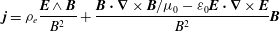 $$\begin{eqnarray}\displaystyle & \displaystyle \boldsymbol{j}=\unicode[STIX]{x1D70C}_{e}\frac{\boldsymbol{E}\wedge \boldsymbol{B}}{B^{2}}+\frac{\boldsymbol{B}\boldsymbol{\cdot }\unicode[STIX]{x1D735}\times \boldsymbol{B}/\unicode[STIX]{x1D707}_{0}-\unicode[STIX]{x1D700}_{0}\boldsymbol{E}\boldsymbol{\cdot }\unicode[STIX]{x1D735}\times \boldsymbol{E}}{B^{2}}\boldsymbol{B} & \displaystyle\end{eqnarray}$$
 $$\begin{eqnarray}\displaystyle & \displaystyle \unicode[STIX]{x1D70C}_{e}=\unicode[STIX]{x1D700}_{0}\unicode[STIX]{x1D735}\boldsymbol{\cdot }\boldsymbol{E}. & \displaystyle\end{eqnarray}$$
 $r_{L}$
. Note that in all these simulations, no account of the current parallel to the magnetic field is taken, only the electric drift current, the term proportional to
$r_{L}$
. Note that in all these simulations, no account of the current parallel to the magnetic field is taken, only the electric drift current, the term proportional to
 $\boldsymbol{E}\wedge \boldsymbol{B}$
in expression (5.1a
) is in fact computed, a limitation due to the finite difference scheme they used. The force-free aligned rotator has been reinvestigated by several authors such as Gruzinov (Reference Gruzinov2005), McKinney (Reference McKinney2006) and Timokhin (Reference Timokhin2006). An analytical study of the influence of relativistic space charge limited outflow was undertaken by Muslimov & Harding (Reference Muslimov and Harding2005). Lastly, the computation of light curves associated with these simulations performed by Kalapotharakos et al. (Reference Kalapotharakos, Harding, Kazanas and Contopoulos2012b
) offers an efficient test to check the conjectured hypothesis. Goodwin et al. (Reference Goodwin, Mestel, Mestel and Wright2004) attempted to look analytically at non-dissipative force-free magnetospheres using Fourier transform techniques in two dimensions.
$\boldsymbol{E}\wedge \boldsymbol{B}$
in expression (5.1a
) is in fact computed, a limitation due to the finite difference scheme they used. The force-free aligned rotator has been reinvestigated by several authors such as Gruzinov (Reference Gruzinov2005), McKinney (Reference McKinney2006) and Timokhin (Reference Timokhin2006). An analytical study of the influence of relativistic space charge limited outflow was undertaken by Muslimov & Harding (Reference Muslimov and Harding2005). Lastly, the computation of light curves associated with these simulations performed by Kalapotharakos et al. (Reference Kalapotharakos, Harding, Kazanas and Contopoulos2012b
) offers an efficient test to check the conjectured hypothesis. Goodwin et al. (Reference Goodwin, Mestel, Mestel and Wright2004) attempted to look analytically at non-dissipative force-free magnetospheres using Fourier transform techniques in two dimensions.
Let us emphasize some drawbacks of the first ever 3-D simulations.
-
(i) The ratio
$R/r_{L}=0.2$
is too large, it corresponds to an unrealistic pulsar of period as low as 1 ms. -
(ii) The Cartesian geometry does not permit a satisfactory treatment of boundary conditions at the stellar surface.
-
(iii) The outer bound of the numerical box leads to inconvenient reflections polluting the interior of the domain for long time runs.
-
(iv) These simulations use
$\boldsymbol{E}\boldsymbol{\cdot }\boldsymbol{B}$
cleaning techniques which in effect introduces a parallel electric current that shorts out this
$\boldsymbol{E}\boldsymbol{\cdot }\boldsymbol{B}$
. This method serves the same purpose as the parallel electric current term in (5.1a
). -
(v) A current sheet forms, separating field lines attached to the north pole from those attached to the south pole. It represents a singular surface difficult to catch numerically and physically not realistic. The ideal MHD or force-free approximation fails, dissipation should play an important role in this current sheet.


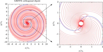
Figure 7. Magnetospheric structure of the perpendicular rotator for a general-relativistic dipole magnetic field with
 $R/r_{L}=0.2$
and
$R/r_{L}=0.2$
and
 $R/R_{s}=2$
. The distances are normalized to the light-cylinder radius. A spiral arm forms where field lines change polarity. This special geometry is at the heart of the striped wind model, § 7.
$R/R_{s}=2$
. The distances are normalized to the light-cylinder radius. A spiral arm forms where field lines change polarity. This special geometry is at the heart of the striped wind model, § 7.
Pétri (Reference Pétri2012) has partially eliminated some of these drawbacks by formulating a new algorithm to solve the Maxwell equations with the help of pseudo-spectral methods. The main idea is to expand the unknown fields into vector spherical harmonics. Application examples of this technique in electromagnetism are available in Lambert (Reference Lambert1978) and Barrera, Estevez & Giraldo (Reference Barrera, Estevez and Giraldo1985). At the same time, Parfrey, Beloborodov & Hui (Reference Parfrey, Beloborodov and Hui2012) developed a similar technique but only in an axisymmetric geometry that was recently reinvestigated by Cao, Zhang & Sun (Reference Cao, Zhang and Sun2016b ). The superiority of this novel method is indisputable, from the point of view of numerical precision, boundary condition treatment and computational resources. The perpendicular rotator is shown in figure 7, the structure of the magnetic field lines in the equatorial plane are visible as the red solid lines. To ease the comparison with the vacuum rotator, we overlap the two-armed spiral in the blue solid line in order to localize the discontinuity. Adjustment is done by eye and it is necessary to add a small phase shift with respect to the vacuum to correctly reproduce the sheet. From the force-free simulations, the power radiated by Poynting flux for an oblique rotator can be deduced and fitted with a simple relation
 $$\begin{eqnarray}\displaystyle L_{sp}\approx {\textstyle \frac{3}{2}}L_{\bot }^{vac}(1+\sin ^{2}\unicode[STIX]{x1D712}) & & \displaystyle\end{eqnarray}$$
in agreement with Spitkovsky (Reference Spitkovsky2006). The presence of a magnetospheric plasma multiplies by three these losses compared to vacuum. The aligned rotator also radiates at a rate of
 $L_{sp}\approx \frac{3}{2}L_{\bot }^{vac}$
. This contrasts radically with the solution for an aligned rotator in vacuum which does not radiate. Moreover Pétri (Reference Pétri2012) demonstrated that the total charge of the star
$L_{sp}\approx \frac{3}{2}L_{\bot }^{vac}$
. This contrasts radically with the solution for an aligned rotator in vacuum which does not radiate. Moreover Pétri (Reference Pétri2012) demonstrated that the total charge of the star
 $+$
magnetosphere system does not vanish except in the particular case of a perpendicular rotator. This is reminiscent of the point charge located at the stellar centre (2.12). It is questionable how such a charge could subsist without cancellation by attraction of particles of the opposite sign from the surroundings. To conclude regarding simulations, the luminosity of a plasma filled magnetosphere is of the same order of magnitude as the dipole in vacuum. It is therefore delicate to make a definite distinction observationally between these two models simply by inspection of the power radiated.
$+$
magnetosphere system does not vanish except in the particular case of a perpendicular rotator. This is reminiscent of the point charge located at the stellar centre (2.12). It is questionable how such a charge could subsist without cancellation by attraction of particles of the opposite sign from the surroundings. To conclude regarding simulations, the luminosity of a plasma filled magnetosphere is of the same order of magnitude as the dipole in vacuum. It is therefore delicate to make a definite distinction observationally between these two models simply by inspection of the power radiated.
5.2 Resistive force-free electrodynamics
The current sheet appearing in the above mentioned simulations is an artefact of the force-free approximation. It would also appear in ideal MHD simulations. In this region, a non-negligible resistivity should soften the discontinuity. The force-free electrodynamics in its simplest form does not allow for dissipation in the flow because it corresponds to an infinite conductivity. Although this should not be such a drawback for the global magnetospheric structure, it is really difficult to elucidate locally the location of emission regions where particle acceleration occurs and radiation is produced. The force-free approximation cannot account for particle acceleration nor for pulsed emission in the magnetosphere. This impossibility goes back to the condition
 $\boldsymbol{E}\boldsymbol{\cdot }\boldsymbol{B}=0$
which is too restrictive. We should allow for a
$\boldsymbol{E}\boldsymbol{\cdot }\boldsymbol{B}=0$
which is too restrictive. We should allow for a
 $E_{\Vert }$
and/or for regions where
$E_{\Vert }$
and/or for regions where
 $E>cB$
. Such prescriptions have been proposed for the current in the magnetosphere, alleviating the prescription in (5.1a
). This requires a parallel electric field that by the force-free assumption does not exist. To circumvent this disadvantage, some less restrictive magnetodynamics regimes have been developed, a kind of resistive magnetodynamics. Whereas the prescription in the force-free limit leads to a definite and precise expression for the current density, it is less clear how to impose this current when the flow becomes dissipative or resistive. There is no unique prescription to generalize Ohm’s law in this regime. Some degree of freedom is available for the exact expression of the current
$E>cB$
. Such prescriptions have been proposed for the current in the magnetosphere, alleviating the prescription in (5.1a
). This requires a parallel electric field that by the force-free assumption does not exist. To circumvent this disadvantage, some less restrictive magnetodynamics regimes have been developed, a kind of resistive magnetodynamics. Whereas the prescription in the force-free limit leads to a definite and precise expression for the current density, it is less clear how to impose this current when the flow becomes dissipative or resistive. There is no unique prescription to generalize Ohm’s law in this regime. Some degree of freedom is available for the exact expression of the current
 $\boldsymbol{j}$
. Several examples of a kind of generalized resistive Ohm’s law for a relativistic pair plasma have been suggested by Lyutikov (Reference Lyutikov2003), Li, Spitkovsky & Tchekhovskoy (Reference Li, Spitkovsky and Tchekhovskoy2012b
) and Kalapotharakos et al. (Reference Kalapotharakos, Kazanas, Harding and Contopoulos2012c
). Gruzinov (Reference Gruzinov2008) proposed an approximation called strong field electrodynamics giving the current as
$\boldsymbol{j}$
. Several examples of a kind of generalized resistive Ohm’s law for a relativistic pair plasma have been suggested by Lyutikov (Reference Lyutikov2003), Li, Spitkovsky & Tchekhovskoy (Reference Li, Spitkovsky and Tchekhovskoy2012b
) and Kalapotharakos et al. (Reference Kalapotharakos, Kazanas, Harding and Contopoulos2012c
). Gruzinov (Reference Gruzinov2008) proposed an approximation called strong field electrodynamics giving the current as
 $$\begin{eqnarray}\displaystyle \boldsymbol{j}=\frac{\unicode[STIX]{x1D70C}_{e}\boldsymbol{E}\wedge \boldsymbol{B}+\sqrt{\unicode[STIX]{x1D70C}_{e}^{2}+\unicode[STIX]{x1D6FE}^{2}\unicode[STIX]{x1D70E}^{2}E_{0}^{2}/c^{2}}(E_{0}\boldsymbol{E}/c+cB_{0}\boldsymbol{B})}{B^{2}+E_{0}^{2}/c^{2}}. & & \displaystyle\end{eqnarray}$$
The
 $\unicode[STIX]{x1D70E}$
parameter cannot be interpreted as a conductivity because for
$\unicode[STIX]{x1D70E}$
parameter cannot be interpreted as a conductivity because for
 $\unicode[STIX]{x1D70E}=0$
the vacuum case is not retrieved. Actually this expression is valid for a plasma entirely charge separated and subject to radiation reaction in the ultra-relativistic regime, see below. Indeed, for
$\unicode[STIX]{x1D70E}=0$
the vacuum case is not retrieved. Actually this expression is valid for a plasma entirely charge separated and subject to radiation reaction in the ultra-relativistic regime, see below. Indeed, for
 $\unicode[STIX]{x1D70E}=0$
we found
$\unicode[STIX]{x1D70E}=0$
we found
 $$\begin{eqnarray}\displaystyle \boldsymbol{j}=\frac{\unicode[STIX]{x1D70C}_{e}\boldsymbol{E}\wedge \boldsymbol{B}+|\unicode[STIX]{x1D70C}_{e}|(E_{0}\boldsymbol{E}/c+cB_{0}\boldsymbol{B})}{B^{2}+E_{0}^{2}/c^{2}}. & & \displaystyle\end{eqnarray}$$
Another approximation consists of writing Ohm’s law in the fluid rest frame where the electric and magnetic fields are aligned and then Lorentz transformed to the laboratory frame. In such a way Li et al. (Reference Li, Spitkovsky and Tchekhovskoy2012b
) found an expression function of the fluid velocity along the field lines,
 $\unicode[STIX]{x1D6FD}_{\Vert }c$
which remains undetermined, such that
$\unicode[STIX]{x1D6FD}_{\Vert }c$
which remains undetermined, such that
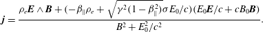 $$\begin{eqnarray}\displaystyle \boldsymbol{j}=\frac{\unicode[STIX]{x1D70C}_{e}\boldsymbol{E}\wedge \boldsymbol{B}+(-\unicode[STIX]{x1D6FD}_{\Vert }\unicode[STIX]{x1D70C}_{e}+\sqrt{\unicode[STIX]{x1D6FE}^{2}(1-\unicode[STIX]{x1D6FD}_{\Vert }^{2})}\unicode[STIX]{x1D70E}E_{0}/c)(E_{0}\boldsymbol{E}/c+cB_{0}\boldsymbol{B})}{B^{2}+E_{0}^{2}/c^{2}}. & & \displaystyle\end{eqnarray}$$
The minimal hypothesis they chose was to set
 $\unicode[STIX]{x1D6FD}_{\Vert }=0$
for lack of better knowledge about the longitudinal speed. The current then simplifies to
$\unicode[STIX]{x1D6FD}_{\Vert }=0$
for lack of better knowledge about the longitudinal speed. The current then simplifies to
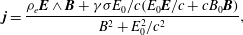 $$\begin{eqnarray}\displaystyle \boldsymbol{j}=\frac{\unicode[STIX]{x1D70C}_{e}\boldsymbol{E}\wedge \boldsymbol{B}+\unicode[STIX]{x1D6FE}\unicode[STIX]{x1D70E}E_{0}/c(E_{0}\boldsymbol{E}/c+cB_{0}\boldsymbol{B})}{B^{2}+E_{0}^{2}/c^{2}}, & & \displaystyle\end{eqnarray}$$
which is Ohm’s law for a relativistic quasi-neutral plasma
 $$\begin{eqnarray}\displaystyle \boldsymbol{j}=\unicode[STIX]{x1D6FE}\unicode[STIX]{x1D70E}(\boldsymbol{E}+\boldsymbol{v}\wedge \boldsymbol{B}-(\boldsymbol{E}\boldsymbol{\cdot }\boldsymbol{v})\boldsymbol{v})+\unicode[STIX]{x1D70C}_{e}\boldsymbol{v}, & & \displaystyle\end{eqnarray}$$
with a drift speed given by
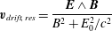 $$\begin{eqnarray}\displaystyle \boldsymbol{v}_{drift,\,res}=\frac{\boldsymbol{E}\wedge \boldsymbol{B}}{B^{2}+E_{0}^{2}/c^{2}} & & \displaystyle\end{eqnarray}$$
and an associated Lorentz factor
 $$\begin{eqnarray}\displaystyle \unicode[STIX]{x1D6FE}^{2}=\frac{E_{0}^{2}+c^{2}B^{2}}{E_{0}^{2}+c^{2}B_{0}^{2}}. & & \displaystyle\end{eqnarray}$$
The current is then exactly the one obtained from the minimal hypothesis with
 $\unicode[STIX]{x1D6FD}_{\Vert }=0$
. The origin of the conductivity was not explicitly stated in these works but turbulence in a relativistic plasma could account for sharp variation of the effective conductivity within the magnetosphere. According to Kaplan, Tsytovich & Éidman (Reference Kaplan, Tsytovich and Éidman1974) the conductivity increases with distance to the star, which is opposite to the force-free inside dissipative outside (FIDO) model used by Kalapotharakos, Harding & Kazanas (Reference Kalapotharakos, Harding and Kazanas2014). The latter work used an Ohm law given by
$\unicode[STIX]{x1D6FD}_{\Vert }=0$
. The origin of the conductivity was not explicitly stated in these works but turbulence in a relativistic plasma could account for sharp variation of the effective conductivity within the magnetosphere. According to Kaplan, Tsytovich & Éidman (Reference Kaplan, Tsytovich and Éidman1974) the conductivity increases with distance to the star, which is opposite to the force-free inside dissipative outside (FIDO) model used by Kalapotharakos, Harding & Kazanas (Reference Kalapotharakos, Harding and Kazanas2014). The latter work used an Ohm law given by
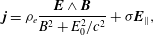 $$\begin{eqnarray}\displaystyle \boldsymbol{j}=\unicode[STIX]{x1D70C}_{e}\frac{\boldsymbol{E}\wedge \boldsymbol{B}}{B^{2}+E_{0}^{2}/c^{2}}+\unicode[STIX]{x1D70E}\boldsymbol{E}_{\Vert }, & & \displaystyle\end{eqnarray}$$
which has been re-explored using spectral methods by Cao, Zhang & Sun (Reference Cao, Zhang and Sun2016a ). Earlier attempts to design a generalized Ohm law are given by Burman (Reference Burman1977a ,Reference Burman c ). Switching between a vacuum and high conducting magnetosphere furnishes an explanation for the braking index variation during on and off states (Li, Spitkovsky & Tchekhovskoy Reference Li, Spitkovsky and Tchekhovskoy2012a ).
5.3 Ideal and resistive MHD
Since the determination of this resistivity is debated, it seems more judicious to relax the resistive magnetodynamics condition and explore the MHD realm, including particle inertia and even pressure, as for the aligned rotator which is also a more realistic approach. We can also take advantage of the remarks made by Komissarov (Reference Komissarov2006). The most satisfactory method would certainly require a multi-fluid, or better, a kinetic approach. The MHD approach to the pulsar magnetosphere was performed by Tchekhovskoy, Spitkovsky & Li (Reference Tchekhovskoy, Spitkovsky and Li2013). Kojima & Oogi (Reference Kojima and Oogi2009) adopted this multi-fluid track performing two-fluid cold plasma simulations but so far only for the aligned rotator. An analytical description of a two-fluid axisymmetric pulsar magnetosphere is given by Petrova (Reference Petrova2015). Resistive methods are usually constrained by stiff source terms depending on the conductivity parameter. Such difficulties are overcome by introducing implicit–explicit Runge–Kutta (IMEX) schemes, as implemented by Palenzuela (Reference Palenzuela2013). MHD types of wave exist in pulsar magnetospheres but need to take the charge density into account (Urpin Reference Urpin2011). Simulations of monopoles and axisymmetric dipoles performed by Bucciantini et al. (Reference Bucciantini, Thompson, Arons, Quataert and Del Zanna2006) revealed that, depending on the resistivity, the location of the Y-point can shift well inside the light cylinder, modifying the spin-down rate from the standard acceptance that
 $R_{Y}=r_{L}$
.
$R_{Y}=r_{L}$
.
5.4 Kinetic methods
The full description of the plasma would require solution of the Vlasov–Maxwell equations which offer the most detailed view of the magnetospheric plasma configuration and allow deep diagnostics of particle acceleration regions. Unfortunately these equations are numerically very difficult to solve because the distribution functions are defined in six dimensions, three space coordinates and three momenta coordinates. A less stringent technique employs particle in cell (PIC) methods. They were successfully applied by Wada & Shibata (Reference Wada and Shibata2007) to elucidate the link between the active magnetosphere and the pulsar wind by including a possible pair creation mechanism with radiation reaction forces. These works were taken up later with a better resolution and a higher number of particles by Wada & Shibata (Reference Wada and Shibata2011). They set-up an electrostatic approximation, neglecting the feedback of the current onto the magnetic field, supposed dipolar and immutable. However, this is justified only when the magnetospheric current density is weak. Yuki & Shibata (Reference Yuki and Shibata2012) described very similar studies. Umizaki & Shibata (Reference Umizaki and Shibata2010) focused on a detailed study of the Y-point in the aligned rotator, i.e. the cusp point of the last field line just grazing the light cylinder. These PIC methods are indisputably much more promising to model the pulsar magnetosphere.
Starting with a full 3-D PIC code, Philippov & Spitkovsky (Reference Philippov and Spitkovsky2014) studied axisymmetric configurations. Then Philippov, Spitkovsky & Cerutti (Reference Philippov, Spitkovsky and Cerutti2015b ) presented 3-D PIC simulations of the pulsar magnetosphere with conclusions very similar to the MHD magnetosphere simulations performed by Tchekhovskoy et al. (Reference Tchekhovskoy, Spitkovsky and Li2013). Chen & Beloborodov (Reference Chen and Beloborodov2014) used PIC simulations and included pair creation from the polar cap up to the light cylinder to look at the filling properties of the magnetosphere. They found solutions very similar to the force-free limit for large pair injection but relaxation to an electrosphere for too low injection rates. Belyaev (Reference Belyaev2015) looked at the transfer of energy between the Poynting flux and the particle. He found that approximately 20 % goes into particle acceleration and up to 50 % if the electric field is not sufficiently screened by the presence of a plasma. Similarly, Cerutti et al. (Reference Cerutti, Philippov, Parfrey and Spitkovsky2015) performed 2-D axisymmetric PIC simulations of the aligned rotator to look at particle acceleration in the equatorial plane containing the current sheet (that otherwise in 3-D would be called the striped wind part). Depending on the particle injection rate, they found that up to 30 % of the magnetic energy is dissipated within several light-cylinder radii.
Very recently, first attempts have been made by Cerutti, Philippov & Spitkovsky (Reference Cerutti, Philippov and Spitkovsky2016) to include radiation reaction self-consistently into a fully 3-D PIC code in order to observe particle acceleration and jointly to extract light curves. PIC simulations do not put particles arbitrary into the magnetosphere as does the force-free approximation but instead rely on a more microphysical explanation of pair creation. The crucial point is to adjust the efficiency to realistic values that are unfortunately largely unconstrained.
5.5 GRFFE
The trend to move to more quantitatively accurate magnetospheres via numerical simulations requires more physical inputs to catch the full complexity of pulsar electrodynamics. General-relativistic effects should be accounted for to obtain a precision better than 20 %. As the quality and quantity of multi-wavelength observations increased drastically over the last decades, those refinements have become compulsory. The 3+1 formalism has been extensively used to compute general relativistic force-free solutions for neutron star magnetosphere. Vacuum solution are of the Deutsch kind but in general relativity are discussed in Pétri (Reference Pétri2013a ). The numerical simulations based on a pseudo-spectral code are described in Pétri (Reference Pétri2014) and extended to a discontinuous Galerkin approach in Pétri (Reference Pétri2015c , Reference Pétri2016a ). The conclusions drawn from special-relativistic force-free (SRFFE) simulations remain valid and the physics is not changed. However, frame dragging seems to be required to enhance the pair production in the polar caps (Philippov et al. Reference Philippov, Cerutti, Tchekhovskoy and Spitkovsky2015a ) to obtain sufficiently high plasma densities. Rayimbaev et al. (Reference Rayimbaev, Ahmedov, Juraeva and Rakhmatov2015) proposed general-relativistic corrections to the charge density along open field lines in the slow rotation approximation and including a possible deformation of the star.
5.6 GRFFQED
QED effects are compulsory on a microscopic scale to trigger pair cascades in the strong magnetic field of a neutron star. Single or multiple photon interactions and disintegration into leptons are the main channels to feed the magnetosphere with a plasma. The question arises as to the effect of these strong fields on the macroscopic scale, of the order the light-cylinder radius. Currently, investigations have been performed to account for lowest-order corrections induced by QED to the total spin-down luminosity and electromagnetic field structure around neutron stars. Because the corrections remain weak, less than the fine structure constant for field strengths
 $B\leqslant 10^{10}$
T, preliminary results for vacuum rotators show that QED effects are irrelevant as far as the global dynamics is concerned (Petri Reference Petri2016). Plasma effects in the force-free regime are also investigated but no drastic changes are found compared to vacuum.
$B\leqslant 10^{10}$
T, preliminary results for vacuum rotators show that QED effects are irrelevant as far as the global dynamics is concerned (Petri Reference Petri2016). Plasma effects in the force-free regime are also investigated but no drastic changes are found compared to vacuum.
5.7 Radiation reaction limit
To date, fluid simulations have treated radiation in a post-processing fashion, after computing the magnetosphere structure in a force-free, MHD or resistive approximation. There is no back reaction of emission onto particle dynamics. Because pulsar magnetospheres contain ultra-relativistic particles radiating copiously at all wavelengths, radiative corrections to particle trajectories can be easily treated in the radiation reaction limit assuming a stationary balance between acceleration and emission. Indeed, in the electromagnetic field prevailing in the pulsar magnetosphere, the plasma suffers strong radiation reaction, invalidating the condition
 $\boldsymbol{E}\boldsymbol{\cdot }\boldsymbol{B}=0$
. Particles are braked and feel a kind of frictional force directed opposite to their velocity such that
$\boldsymbol{E}\boldsymbol{\cdot }\boldsymbol{B}=0$
. Particles are braked and feel a kind of frictional force directed opposite to their velocity such that
 $\boldsymbol{f}_{rad}=-K\boldsymbol{v}$
. By definition, the constant
$\boldsymbol{f}_{rad}=-K\boldsymbol{v}$
. By definition, the constant
 $K$
is positive and can be derived explicitly as follows. In a stationary regime, a particle of charge
$K$
is positive and can be derived explicitly as follows. In a stationary regime, a particle of charge
 $q$
is pulled by Lorentz and radiation reaction forces such that
$q$
is pulled by Lorentz and radiation reaction forces such that
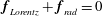 $\boldsymbol{f}_{Lorentz}+\boldsymbol{f}_{rad}=0$
or
$\boldsymbol{f}_{Lorentz}+\boldsymbol{f}_{rad}=0$
or
 $$\begin{eqnarray}\displaystyle q(\boldsymbol{E}+\boldsymbol{v}\wedge \boldsymbol{B})=K\boldsymbol{v}. & & \displaystyle\end{eqnarray}$$
Following the reasoning of Mestel (Reference Mestel1999) it is possible to derive the speed of any particle in a prescribed electromagnetic field in the limit where its speed is equal to c, which is a good approximation in pulsar magnetospheres. We notice that
 $$\begin{eqnarray}\displaystyle q\boldsymbol{E}\boldsymbol{\cdot }\boldsymbol{B}=K\boldsymbol{v}\boldsymbol{\cdot }\boldsymbol{B}\neq 0. & & \displaystyle\end{eqnarray}$$
The constant
 $K$
is solution of
$K$
is solution of
 $$\begin{eqnarray}\displaystyle K^{4}v^{2}-q^{2}(E^{2}-v^{2}B^{2})K^{2}-q^{4}(\boldsymbol{E}\boldsymbol{\cdot }\boldsymbol{B})^{2}=0 & & \displaystyle\end{eqnarray}$$
assuming that the speed of the particles are near to speed of light, we solve for
 $K$
to obtain
$K$
to obtain
 $$\begin{eqnarray}\displaystyle K^{2}\approx \frac{q^{2}}{2c^{2}}\left[E^{2}-c^{2}B^{2}\pm \sqrt{(E^{2}-c^{2}B^{2})^{2}+4c^{2}(\boldsymbol{E}\boldsymbol{\cdot }\boldsymbol{ B})^{2}}\right]. & & \displaystyle\end{eqnarray}$$
The solution with negative sign has to be rejected because
 $K^{2}<0$
.
$K^{2}<0$
.
 $K$
is the solution of the following Lorentz invariant system
$K$
is the solution of the following Lorentz invariant system
 $$\begin{eqnarray}\displaystyle & \displaystyle E^{2}-c^{2}B^{2}=c^{2}K^{2}/q^{2}-c^{2}B_{0}^{2} & \displaystyle\end{eqnarray}$$
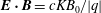 $$\begin{eqnarray}\displaystyle & \displaystyle \boldsymbol{E}\boldsymbol{\cdot }\boldsymbol{B}=cKB_{0}/|q| & \displaystyle\end{eqnarray}$$
 $cK/|q|$
represents the intensity of the electric field in the frame where the electric and magnetic fields are aligned. The constant
$cK/|q|$
represents the intensity of the electric field in the frame where the electric and magnetic fields are aligned. The constant
 $cK/|q|>0$
can be linked to the previous discussion about resistive force-free electrodynamics. In that section it was depicted by the letter
$cK/|q|>0$
can be linked to the previous discussion about resistive force-free electrodynamics. In that section it was depicted by the letter
 $E_{0}$
.
$E_{0}$
.
In the special case where
 $\boldsymbol{E}\boldsymbol{\cdot }\boldsymbol{B}=0$
we get for
$\boldsymbol{E}\boldsymbol{\cdot }\boldsymbol{B}=0$
we get for
 $E<cB$
the condition
$E<cB$
the condition
 $K^{2}=0$
and for
$K^{2}=0$
and for
 $E>cB$
the condition
$E>cB$
the condition
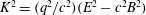 $K^{2}=(q^{2}/c^{2})(E^{2}-c^{2}B^{2})$
. In the case of a general weak electric field,
$K^{2}=(q^{2}/c^{2})(E^{2}-c^{2}B^{2})$
. In the case of a general weak electric field,
 $E\ll cB$
then
$E\ll cB$
then
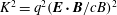 $K^{2}=q^{2}(\boldsymbol{E}\boldsymbol{\cdot }\boldsymbol{B}/cB)^{2}$
. Solving for the speed starting from (5.11) and using (5.12) we obtain
$K^{2}=q^{2}(\boldsymbol{E}\boldsymbol{\cdot }\boldsymbol{B}/cB)^{2}$
. Solving for the speed starting from (5.11) and using (5.12) we obtain
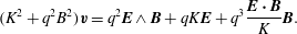 $$\begin{eqnarray}\displaystyle (K^{2}+q^{2}B^{2})\boldsymbol{v}=q^{2}\boldsymbol{E}\wedge \boldsymbol{B}+qK\boldsymbol{E}+q^{3}\frac{\boldsymbol{E}\boldsymbol{\cdot }\boldsymbol{B}}{K}\boldsymbol{B}. & & \displaystyle\end{eqnarray}$$
The velocity can be decomposed into a drift motion superposed to a motion along
 $\boldsymbol{E}$
and
$\boldsymbol{E}$
and
 $\boldsymbol{B}$
such that
$\boldsymbol{B}$
such that
 $$\begin{eqnarray}\displaystyle & \displaystyle \boldsymbol{v}_{drift,\,rr}=\frac{\boldsymbol{E}\wedge \boldsymbol{B}}{E_{0}^{2}/c^{2}+B^{2}} & \displaystyle\end{eqnarray}$$
 $$\begin{eqnarray}\displaystyle & \displaystyle \boldsymbol{v}_{EB,\,rr}=\text{sign}(q)\frac{E_{0}\boldsymbol{E}/c^{2}+B_{0}\boldsymbol{B}}{E_{0}^{2}/c^{2}+B^{2}}. & \displaystyle\end{eqnarray}$$
 $\boldsymbol{v}=\text{sign}(q)c\boldsymbol{E}/E$
as expected from an almost instantaneous acceleration on a time scale much shorter than any other dynamical time (zero inertia limit). These results regarding the speed of particles in the radiation reaction limit have already been given by Herold, Ertl & Ruder (Reference Herold, Ertl and Ruder1985) and Finkbeiner et al. (Reference Finkbeiner, Herold, Ertl and Ruder1989) who also solve numerically the equation of motion including radiation reaction. Finkbeiner, Herold & Ruder (Reference Finkbeiner, Herold and Ruder1990) discussed the validity of the Lorentz–Dirac equation in pulsar magnetospheres. A detailed study by Laue & Thielheim (Reference Laue and Thielheim1986) integrating numerically the Lorentz–Dirac equation for electrons and protons showed the particle orbits and maximum attainable energy for a perpendicular rotator. The radiation reaction limit, much is simpler to implement as the full equation of motion, has been applied to solve the pulsar magnetosphere topology by Gruzinov (Reference Gruzinov2012), Gruzinov (Reference Gruzinov2013) and Contopoulos (Reference Contopoulos2016a
). They claim that two types of pulsars should exist: those that are very dissipative and those that are not. Ferrari & Trussoni (Reference Ferrari and Trussoni1974) studied radiation reaction in pulsar magnetospheres and also in the context of cosmic ray acceleration.
$\boldsymbol{v}=\text{sign}(q)c\boldsymbol{E}/E$
as expected from an almost instantaneous acceleration on a time scale much shorter than any other dynamical time (zero inertia limit). These results regarding the speed of particles in the radiation reaction limit have already been given by Herold, Ertl & Ruder (Reference Herold, Ertl and Ruder1985) and Finkbeiner et al. (Reference Finkbeiner, Herold, Ertl and Ruder1989) who also solve numerically the equation of motion including radiation reaction. Finkbeiner, Herold & Ruder (Reference Finkbeiner, Herold and Ruder1990) discussed the validity of the Lorentz–Dirac equation in pulsar magnetospheres. A detailed study by Laue & Thielheim (Reference Laue and Thielheim1986) integrating numerically the Lorentz–Dirac equation for electrons and protons showed the particle orbits and maximum attainable energy for a perpendicular rotator. The radiation reaction limit, much is simpler to implement as the full equation of motion, has been applied to solve the pulsar magnetosphere topology by Gruzinov (Reference Gruzinov2012), Gruzinov (Reference Gruzinov2013) and Contopoulos (Reference Contopoulos2016a
). They claim that two types of pulsars should exist: those that are very dissipative and those that are not. Ferrari & Trussoni (Reference Ferrari and Trussoni1974) studied radiation reaction in pulsar magnetospheres and also in the context of cosmic ray acceleration.
From this general expression of the particle velocity in an electromagnetic field, we can prescribe an electric current density including the motion of electrons and positrons. Considering a reference particle density number
 $n_{0}$
and introducing the pair multiplicity parameter by
$n_{0}$
and introducing the pair multiplicity parameter by
 $\unicode[STIX]{x1D705}$
, the charge density
$\unicode[STIX]{x1D705}$
, the charge density
 $\unicode[STIX]{x1D70C}_{e}$
is deduced from Maxwell–Gauss equation and furnishes the reference particle number density. Let us use
$\unicode[STIX]{x1D70C}_{e}$
is deduced from Maxwell–Gauss equation and furnishes the reference particle number density. Let us use
 $n_{0}$
as a free parameter such that
$n_{0}$
as a free parameter such that
 $$\begin{eqnarray}\displaystyle & \displaystyle \unicode[STIX]{x1D70C}_{e}=\unicode[STIX]{x1D700}_{0}\unicode[STIX]{x1D735}\boldsymbol{\cdot }\boldsymbol{E} & \displaystyle\end{eqnarray}$$
 $$\begin{eqnarray}\displaystyle & \displaystyle en=|\unicode[STIX]{x1D70C}_{e}| & \displaystyle\end{eqnarray}$$
 $$\begin{eqnarray}\displaystyle & \displaystyle \unicode[STIX]{x1D70C}_{e}=e(n_{+}-n_{-}) & \displaystyle\end{eqnarray}$$
 $$\begin{eqnarray}\displaystyle & \displaystyle \boldsymbol{j}=e(n_{+}\boldsymbol{v}_{+}-n_{-}\boldsymbol{v}_{-}) & \displaystyle\end{eqnarray}$$
 $n$
corresponds to the particle density required for the minimal hypothesis of a totally charge separated plasma. In order to estimate the particle density number, we start from a fully charge separated plasma and add neutral pairs
$n$
corresponds to the particle density required for the minimal hypothesis of a totally charge separated plasma. In order to estimate the particle density number, we start from a fully charge separated plasma and add neutral pairs
 $e^{\pm }$
with a multiplicity
$e^{\pm }$
with a multiplicity
 $\unicode[STIX]{x1D705}$
. We must distinguish between two kinds of regions. If the space charge is positive we choose a background electron density null and add pairs. Primary positrons are at a number of
$\unicode[STIX]{x1D705}$
. We must distinguish between two kinds of regions. If the space charge is positive we choose a background electron density null and add pairs. Primary positrons are at a number of
 $en=\unicode[STIX]{x1D70C}_{e}$
such that
$en=\unicode[STIX]{x1D70C}_{e}$
such that  $$\begin{eqnarray}\displaystyle & \displaystyle n_{-}=\unicode[STIX]{x1D705}n_{0} & \displaystyle\end{eqnarray}$$
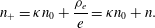 $$\begin{eqnarray}\displaystyle & \displaystyle n_{+}=\unicode[STIX]{x1D705}n_{0}+\frac{\unicode[STIX]{x1D70C}_{e}}{e}=\unicode[STIX]{x1D705}n_{0}+n. & \displaystyle\end{eqnarray}$$
 $en=|\unicode[STIX]{x1D70C}_{e}|$
such that
$en=|\unicode[STIX]{x1D70C}_{e}|$
such that 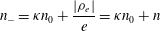 $$\begin{eqnarray}\displaystyle & \displaystyle n_{-}=\unicode[STIX]{x1D705}n_{0}+\frac{|\unicode[STIX]{x1D70C}_{e}|}{e}=\unicode[STIX]{x1D705}n_{0}+n & \displaystyle\end{eqnarray}$$
 $$\begin{eqnarray}\displaystyle & \displaystyle n_{+}=\unicode[STIX]{x1D705}n_{0}. & \displaystyle\end{eqnarray}$$
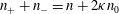 $n_{+}+n_{-}=n+2\unicode[STIX]{x1D705}n_{0}$
. Noting that the speed
$n_{+}+n_{-}=n+2\unicode[STIX]{x1D705}n_{0}$
. Noting that the speed
 $\boldsymbol{v}_{EB}$
of electrons is opposite to that of positrons, because
$\boldsymbol{v}_{EB}$
of electrons is opposite to that of positrons, because
 $K>0$
by assumption and
$K>0$
by assumption and
 $V_{EB}\propto \text{sign}(q)$
, the current becomes
$V_{EB}\propto \text{sign}(q)$
, the current becomes  $$\begin{eqnarray}\displaystyle \boldsymbol{j}=\unicode[STIX]{x1D70C}_{e}\boldsymbol{v}_{drift,\,rr}+(|\unicode[STIX]{x1D70C}_{e}|+2\unicode[STIX]{x1D705}n_{0}e)\boldsymbol{v}_{EB}. & & \displaystyle\end{eqnarray}$$
For a mono-fluid description, we introduce the fluid velocity by
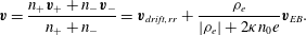 $$\begin{eqnarray}\displaystyle \boldsymbol{v}=\frac{n_{+}\boldsymbol{v}_{+}+n_{-}\boldsymbol{v}_{-}}{n_{+}+n_{-}}=\boldsymbol{v}_{drift,\,rr}+\frac{\unicode[STIX]{x1D70C}_{e}}{|\unicode[STIX]{x1D70C}_{e}|+2\unicode[STIX]{x1D705}n_{0}e}\boldsymbol{v}_{EB}. & & \displaystyle\end{eqnarray}$$
For a quasi-neutral plasma, the pair multiplicity is very high
 $\unicode[STIX]{x1D705}\gg 1$
which means that
$\unicode[STIX]{x1D705}\gg 1$
which means that
 $|n_{+}-n_{-}|\ll n_{+}+n_{-}$
. Therefore
$|n_{+}-n_{-}|\ll n_{+}+n_{-}$
. Therefore
 $|\unicode[STIX]{x1D70C}_{e}|\ll |\unicode[STIX]{x1D70C}_{e}|+2\unicode[STIX]{x1D705}n_{0}e$
and to first approximation the fluid velocity is simply equal to the electric drift motion
$|\unicode[STIX]{x1D70C}_{e}|\ll |\unicode[STIX]{x1D70C}_{e}|+2\unicode[STIX]{x1D705}n_{0}e$
and to first approximation the fluid velocity is simply equal to the electric drift motion
 $\boldsymbol{v}=\boldsymbol{v}_{D}$
. Injecting this expression in Ohm’s relativistic law, we get the current from the minimal hypothesis of (5.6).
$\boldsymbol{v}=\boldsymbol{v}_{D}$
. Injecting this expression in Ohm’s relativistic law, we get the current from the minimal hypothesis of (5.6).
5.8 Observational signature of magnetospheric structure
Remotely diagnosing magnetospheric activity in pulsar physics requires predictions, or better, a posteriori adjustments of dynamical and geometric parameters such as particle injection rate, obliquity of the pulsar and the inclination of the line of sight. Several works in the last decade have tried to match recent gamma-ray light curves obtained from Fermi/LAT (Abdo et al. Reference Abdo, Ajello, Allafort, Baldini, Ballet, Barbiellini, Baring, Bastieri, Belfiore and Bellazzini2013) assuming different plasma regimes. For instance Bai & Spitkovsky (Reference Bai and Spitkovsky2010b ) tested the simple vacuum dipole and compared predicted light curves with observations. In a second trial Bai & Spitkovsky (Reference Bai and Spitkovsky2010a ) used the force-free magnetosphere obtained from previously mentioned simulations with seemingly better fits. Actually, the latter model should not radiate because the force-free model is dissipationless. The location of emission sites is left to the discretion of the physicists. The same and other authors used results from resistive or more generally speaking dissipative prescriptions to compute characteristic pulse profiles (Kalapotharakos et al. Reference Kalapotharakos, Harding, Kazanas and Contopoulos2012b , Reference Kalapotharakos, Harding and Kazanas2014; Brambilla et al. Reference Brambilla, Kalapotharakos, Harding and Kazanas2015). Brambilla et al. (Reference Brambilla, Kalapotharakos, Harding and Kazanas2015) tried to get observational signatures of a dissipative magnetosphere through the computation of gamma-ray light curves. They used the force-free inside dissipative outside (FIDO) model described by Kalapotharakos et al. (Reference Kalapotharakos, Harding and Kazanas2014) to best fit the data. Why no dissipation should apply inside the light cylinder remains mysterious on physical grounds. Full PIC simulations are also starting to predict light curves although results are still preliminary (Cerutti et al. Reference Cerutti, Philippov and Spitkovsky2016). They do not make assumptions about emission sites which are self-consistently determined by the simulations themselves. Sometimes, breakdown of the force-free regime is stated in the vicinity of the light cylinder, allowing efficient particle acceleration and associated intense X-ray and gamma-ray emission (Mestel & Shibata Reference Mestel and Shibata1994). Angular momentum is carried away by the relativistic wind and current closure must occur outside the light cylinder (Shibata Reference Shibata1994). Moreover, possible synchro-Compton emission in the vicinity of the light cylinder was already reported by Ferrari & Trussoni (Reference Ferrari and Trussoni1975).
To summarize in a very condensed way the results obtained so far from numerical simulations of relativistic plasmas in force-free, MHD or kinetic regimes we show the fitted spin-down luminosities in table 3. Note that for all the above mentioned simulation results the Y-point is located at the light cylinder and therefore the spin-down rate implicitly assumes that
 $R_{Y}=r_{L}$
. However according to the axisymmetric FFE magnetosphere constructed by Timokhin (Reference Timokhin2006), this slow down is drastically enhanced when the Y-point is shifted well inside the light cylinder. As claimed by Timokhin (Reference Timokhin2010), the mode changing and nulling of some pulsars could be interpreted by a movable Y-point.
$R_{Y}=r_{L}$
. However according to the axisymmetric FFE magnetosphere constructed by Timokhin (Reference Timokhin2006), this slow down is drastically enhanced when the Y-point is shifted well inside the light cylinder. As claimed by Timokhin (Reference Timokhin2010), the mode changing and nulling of some pulsars could be interpreted by a movable Y-point.
Table 3. Spin-down luminosity expectations from simulations assuming different plasma regimes. The results are
 $f(\unicode[STIX]{x1D712})=f_{0}+f_{1}\sin ^{2}\unicode[STIX]{x1D712}$
with
$f(\unicode[STIX]{x1D712})=f_{0}+f_{1}\sin ^{2}\unicode[STIX]{x1D712}$
with
 $a=R/r_{L}$
and for
$a=R/r_{L}$
and for
 $R=2R_{s}$
in GR. For force-free simulations, the coefficients
$R=2R_{s}$
in GR. For force-free simulations, the coefficients
 $f_{0},f_{1}$
depend slightly on
$f_{0},f_{1}$
depend slightly on
 $a$
, they are not included here but given for
$a$
, they are not included here but given for
 $a=0.1$
.
$a=0.1$
.
6 Electrosphere models
All previous models assumed a magnetosphere entirely filled with a relativistic plasma made essentially of electron–positron pairs at a high multiplicity factor
 $\unicode[STIX]{x1D705}\gg 1$
(but still not enough to fully explain observations). This implies a quasi-neutral state of the plasma. However this configuration is plausibly unstable depending on the rate of particle injection from the polar caps as observed in recent numerical simulations. The simplest idea consists therefore in constructing a nearly corotative electrosphere, that is a magnetosphere partially filled with a non-neutral plasma in which charged particles, from one species or another (electrons, positrons, protons or ions), are present and rotate at a speed close but not equal to that of the star. If this non-neutral plasma enters in solid body rotation with the star, then from a purely electrical point of view, nothing will distinguish this charge separated space region from the star. The neutron star can then equivalently be seen as a larger sphere of radius
$\unicode[STIX]{x1D705}\gg 1$
(but still not enough to fully explain observations). This implies a quasi-neutral state of the plasma. However this configuration is plausibly unstable depending on the rate of particle injection from the polar caps as observed in recent numerical simulations. The simplest idea consists therefore in constructing a nearly corotative electrosphere, that is a magnetosphere partially filled with a non-neutral plasma in which charged particles, from one species or another (electrons, positrons, protons or ions), are present and rotate at a speed close but not equal to that of the star. If this non-neutral plasma enters in solid body rotation with the star, then from a purely electrical point of view, nothing will distinguish this charge separated space region from the star. The neutron star can then equivalently be seen as a larger sphere of radius
 $R_{el}$
introduced in the braking index (2.24). The impossibility of exceeding the speed of light and the hypothesis of synchronous solid body rotation show that this electrosphere cannot extend farther than the radius of the light cylinder. Its extension could be even less if the plasma is in over-rotation, as found in simulations from the mid 1980s and in early 2000. Curiously, electrospheres are neither well known nor seriously studied by authors interested in pulsar physics. We note useful characteristics of this atypical model hoping to boost its attractiveness. The properties of the neutron star electrosphere have been extensively studied in Pétri (Reference Pétri2002).
$R_{el}$
introduced in the braking index (2.24). The impossibility of exceeding the speed of light and the hypothesis of synchronous solid body rotation show that this electrosphere cannot extend farther than the radius of the light cylinder. Its extension could be even less if the plasma is in over-rotation, as found in simulations from the mid 1980s and in early 2000. Curiously, electrospheres are neither well known nor seriously studied by authors interested in pulsar physics. We note useful characteristics of this atypical model hoping to boost its attractiveness. The properties of the neutron star electrosphere have been extensively studied in Pétri (Reference Pétri2002).
6.1 Non-neutral plasma behaviour
The electrosphere model possesses a very different behaviour from that of a quasi-neutral plasma filled magnetosphere used in force-free or MHD theory. In an electrosphere, the plasma is non-neutral and shows properties often opposed to those of a neutral plasma. Table 4 summarizes the divergent features of the two kind of plasmas. Among them, we are particularly interested in particle confinement in electromagnetic traps with variable geometry. Depending on the topology of the magnetic and electric fields, let them be absent, constant, monopolar, dipolar or quadrupolar, the volume of the charge separated regions will show various shapes. Table 5 furnishes a list of traps often used by plasma physicists. A pulsar possibly resembles a rotating Terrella. Non-neutral plasmas are well studied in laboratory experiments because they are easy to confine for a long time (Dubin & O’neil Reference Dubin and O’neil1999). There are some analogies between charge separated plasmas and hydrodynamics, as pointed out by Wright (Reference Wright1978) who discussed it in the context of non-neutral pulsar magnetospheres.
Table 4. The differences in behaviour between neutral and non-neutral plasmas.
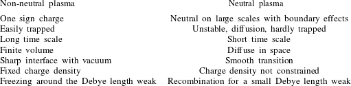
Table 5. Different trapping systems for a non-neutral plasma. Each configuration of the electromagnetic field generates a specific shape of the space-charge distribution.
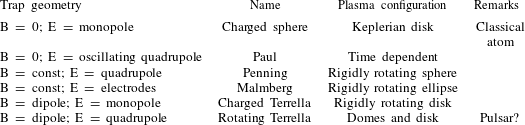
The process of formation of this electrosphere is the followingFootnote 3 . The strongly magnetized and rotating neutron star generates surface and volume charge distributions dictated by the law of electrostatic equilibrium of a perfect conductor in its rest frame. The electric field drags particles out of the surface towards stable equilibrium positions, the so called force-free surfaces (FFS). Particles spread in the immediate stellar surrounding, filling a space charge region forming an extended atmosphere called the electrosphere. The extension of this atmosphere is not dictated by thermal pressure as it would be for the traditional concept of an atmosphere but rather by the electromagnetic forces acting on the charge separated gas. As for the filled magnetosphere, the electrospheric current disturbs the magnetosphere when it approaches the light cylinder. However, if over-rotation is important, as we show below, this feedback could lead to perceptible magnetic perturbations already well within the light cylinder. Moreover, owing to the strong magnetic field, all these particles quickly de-energize to their fundamental Landau level through synchro-photon emission, forbidding any motion perpendicular to magnetic field lines. They are therefore constrained to move along these field lines progressively filling the electrosphere. But then how to fill it? Will charges of opposite sign occupy the same region of space to reach a quasi-neutral state or will they form what we call a charge separated electrosphere where positive and negative zones are exclusively populated by particles of one sign? Let us have a look at different models which attempt to give an answer to this question in a sometimes arbitrary manner.
Given the predominance of electromagnetic forces compared to gravitational forces and any other phenomenon related to particle inertia, it is justified to neglect their mass. Only the Lorentz force exerts a significant action. In electrostatic equilibrium this force vanishes at all places where matter subsists. In this way, in populated regions the law
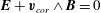 $\boldsymbol{E}+\boldsymbol{v}_{cor}\wedge \boldsymbol{B}=0$
is valid and electric and magnetic field are again perpendicular
$\boldsymbol{E}+\boldsymbol{v}_{cor}\wedge \boldsymbol{B}=0$
is valid and electric and magnetic field are again perpendicular
 $\boldsymbol{E}\boldsymbol{\cdot }\boldsymbol{B}=0$
as inside the star or in the force-free limit. For the sake of simplicity, we ignore relativistic effects, an approximation that is justified for an electrosphere remaining at a reasonable distance from the light cylinder,
$\boldsymbol{E}\boldsymbol{\cdot }\boldsymbol{B}=0$
as inside the star or in the force-free limit. For the sake of simplicity, we ignore relativistic effects, an approximation that is justified for an electrosphere remaining at a reasonable distance from the light cylinder,
 $r\ll r_{L}$
. Some generalisations are conceivable. Building on the method invented by Krause-Polstorff & Michel (Reference Krause-Polstorff and Michel1985b
), Pétri, Heyvaerts & Bonazzola (Reference Pétri, Heyvaerts and Bonazzola2002b
) have shown the existence of such solutions for an aligned rotator, with an extension confined well inside the light cylinder. The solution possesses an equatorial disk in differential rotation and two domes of charge opposite to that of the disk, figure 8. This differential rotation imposes a velocity larger than the stellar rotation, a new but also very important aspect with deep consequences for the stability and long term evolution of such plasmas. A pulsar maybe represents an astrophysical application of particle trapping in a rotating Terrella.
$r\ll r_{L}$
. Some generalisations are conceivable. Building on the method invented by Krause-Polstorff & Michel (Reference Krause-Polstorff and Michel1985b
), Pétri, Heyvaerts & Bonazzola (Reference Pétri, Heyvaerts and Bonazzola2002b
) have shown the existence of such solutions for an aligned rotator, with an extension confined well inside the light cylinder. The solution possesses an equatorial disk in differential rotation and two domes of charge opposite to that of the disk, figure 8. This differential rotation imposes a velocity larger than the stellar rotation, a new but also very important aspect with deep consequences for the stability and long term evolution of such plasmas. A pulsar maybe represents an astrophysical application of particle trapping in a rotating Terrella.
Figure 8. Electrosphere model of an aligned rotator obtained from semi-analytical solutions (Pétri et al. Reference Pétri, Heyvaerts and Bonazzola2002b ).
6.2 Expectations from the model
The corotation of the electrosphere with the star stops at the light cylinder, for
 $r>r_{L}$
or even at shorter distances if over-rotation happens. Several developments have been proposed to replace the notion of corotation and some of them are presented here. An important theorem due to Pilipp (Reference Pilipp1974) derived from not too restrictive assumptions shows that a magnetosphere finite in extent with large vacuum gaps and in force-free equilibrium cannot be in corotation with the star everywhere. As a consequence, differential rotation is an intrinsic property of electrospheres or, more generally speaking, magnetospheres with vacuum gaps (Michel Reference Michel1979). Differential rotation of plasmas around neutron stars was expected since the early days of pulsar theory, as accounted for by the relativistic hydrodynamical study of Hinata & Jackson (Reference Hinata and Jackson1974) who showed the finite extension of the corotation part up to a critical magnetic surface. The trapping regions are defined by the force-free condition
$r>r_{L}$
or even at shorter distances if over-rotation happens. Several developments have been proposed to replace the notion of corotation and some of them are presented here. An important theorem due to Pilipp (Reference Pilipp1974) derived from not too restrictive assumptions shows that a magnetosphere finite in extent with large vacuum gaps and in force-free equilibrium cannot be in corotation with the star everywhere. As a consequence, differential rotation is an intrinsic property of electrospheres or, more generally speaking, magnetospheres with vacuum gaps (Michel Reference Michel1979). Differential rotation of plasmas around neutron stars was expected since the early days of pulsar theory, as accounted for by the relativistic hydrodynamical study of Hinata & Jackson (Reference Hinata and Jackson1974) who showed the finite extension of the corotation part up to a critical magnetic surface. The trapping regions are defined by the force-free condition
 $\boldsymbol{E}\boldsymbol{\cdot }\boldsymbol{B}=0$
corresponding to an extremum in the electrostatic potential (maximum for positive charges and minimum for negative charges). Such sites represent therefore equilibrium places for one species, positive if the potential is minimal or negative if the potential is maximal. These regions are called force-free surfaces (FFS) and have been extensively studied by many authors as a base for the geometry of this electrosphere (Thielheim & Wolfsteller Reference Thielheim and Wolfsteller1989, Reference Thielheim and Wolfsteller1994). Jackson (Reference Jackson1978) emphasized also the notion of the corotational drift surface (CDS) in the arbitrary inclination angle case. Jackson (Reference Jackson1976a
) extensively studied the electrostatic problem of neutron star atmospheres in a series of papers (Jackson Reference Jackson1978, Reference Jackson1979, Reference Jackson1980a
,Reference Jackson
b
, Reference Jackson1981a
,Reference Jackson
b
). Rylov (Reference Rylov1976) computed analytical models of the region around neutron stars filled with electrons and protons/positrons. For the aligned case, he found a proton belt and an electron cap. For a small misalignment he obtained an electron filament current along the poles. He already noted the importance of the total electric charge of the star. He refined his model in several subsequent papers about the electron polar cap shape (Rylov Reference Rylov1977, Reference Rylov1985), electron and particle acceleration (Rylov Reference Rylov1979, Reference Rylov1987,Reference Rylov?) and the influence on pair creation in the magnetosphere (Rylov Reference Rylov1981, Reference Rylov1982, Reference Rylov1984) and the global structure of the magnetosphere (Rylov Reference Rylov1988, Reference Rylov1989). According to this literature, the 1970s and 1980s were the favourable periods to work on the topic discussed in this section.
$\boldsymbol{E}\boldsymbol{\cdot }\boldsymbol{B}=0$
corresponding to an extremum in the electrostatic potential (maximum for positive charges and minimum for negative charges). Such sites represent therefore equilibrium places for one species, positive if the potential is minimal or negative if the potential is maximal. These regions are called force-free surfaces (FFS) and have been extensively studied by many authors as a base for the geometry of this electrosphere (Thielheim & Wolfsteller Reference Thielheim and Wolfsteller1989, Reference Thielheim and Wolfsteller1994). Jackson (Reference Jackson1978) emphasized also the notion of the corotational drift surface (CDS) in the arbitrary inclination angle case. Jackson (Reference Jackson1976a
) extensively studied the electrostatic problem of neutron star atmospheres in a series of papers (Jackson Reference Jackson1978, Reference Jackson1979, Reference Jackson1980a
,Reference Jackson
b
, Reference Jackson1981a
,Reference Jackson
b
). Rylov (Reference Rylov1976) computed analytical models of the region around neutron stars filled with electrons and protons/positrons. For the aligned case, he found a proton belt and an electron cap. For a small misalignment he obtained an electron filament current along the poles. He already noted the importance of the total electric charge of the star. He refined his model in several subsequent papers about the electron polar cap shape (Rylov Reference Rylov1977, Reference Rylov1985), electron and particle acceleration (Rylov Reference Rylov1979, Reference Rylov1987,Reference Rylov?) and the influence on pair creation in the magnetosphere (Rylov Reference Rylov1981, Reference Rylov1982, Reference Rylov1984) and the global structure of the magnetosphere (Rylov Reference Rylov1988, Reference Rylov1989). According to this literature, the 1970s and 1980s were the favourable periods to work on the topic discussed in this section.
6.2.1 Charged wind
The improperly called open field linesFootnote 4 , that is those which do not close inside the light cylinder, let particles escape from the poles. A charged wind made either of positrons/protons/ions or electrons, following the sign of the charge, leaves the magnetosphere from the magnetic poles. The electromagnetic field in the zone of the charged wind finds its source in the current and the distribution of charges induced by these escaping particles. This current, responsible for the loss of charge around both polar caps, should discharge the neutron star. This discharge cannot last for ever, so we must think either of a complete electrostatic equilibrium state or that the current loop closes somewhere in the system. In order to circumvent this difficulty, this current loop should close inside the light cylinder, which is difficult because of the constraint imposed on the particles to stay on drifting orbits along field lines. This difficulty is known as the problem of current closure. This is why Beskin et al. (Reference Beskin, Gurevich and Istomin1983, Reference Beskin, Gurevich and Istomin1993) suggest the notion of an active magnetosphere. A similar argument leading to transfield flows was suggested by Shibata (Reference Shibata1986, Reference Shibata1988).
6.2.2 Active magnetosphere
Given that the current above the poles streams away from the pulsar, a return current must necessarily exist and be pointed towards the pulsar. The current closure is insured thanks to the violation of the electric drift approximation close to the light surface because
 $E>cB$
. Indeed, when approaching this light surface, the drift velocity becomes equal to the speed of light, particle energy increases quickly forcing acceleration and consequently violating the ideal MHD approximation. Electrons and positrons are allowed to cross field lines along this light surface, electrons going in one direction and positrons in the opposite direction. The current closes through the magnetic surface lying on the frontier of the dead zone, the boundary surface separating open from closed field lines.
$E>cB$
. Indeed, when approaching this light surface, the drift velocity becomes equal to the speed of light, particle energy increases quickly forcing acceleration and consequently violating the ideal MHD approximation. Electrons and positrons are allowed to cross field lines along this light surface, electrons going in one direction and positrons in the opposite direction. The current closes through the magnetic surface lying on the frontier of the dead zone, the boundary surface separating open from closed field lines.
6.2.3 Electrostatic equilibrium
The current closure can be avoided if the system evolves towards an electrosphere in equilibrium with an extension less than the light-cylinder radius
 $r_{L}$
. The distribution of atmospheric charges would be in an equilibrium state under the action of the electromagnetic field; an equilibrium that can be qualified as electrostatic. In a second approximation, we can envisage the breakdown of the frozen-in theorem through the development of instabilities allowing the passage of a resistive and turbulent current. The turbulence is an effect felt by each particle in addition to the macroscopic electric field responsible for the drift motion such as microscopic electric fluctuations similar to the microfields responsible for Coulomb collisions, but much more intense. In these conditions particles can exceptionally deviate from the trajectories indicated by field lines. This aspect is related to non-neutral plasma instabilities developing in the electrosphere. This suggestion is also an alternative for the current closure problem. Deviation from a pure equilibrium is required to ignite an electromagnetic activity in the pulsar and to hope to observe emission. Depending on the charge load in this electrosphere, if it almost entirely fills the light cylinder, we could speak about a partially filled magnetosphere but with huge gaps.
$r_{L}$
. The distribution of atmospheric charges would be in an equilibrium state under the action of the electromagnetic field; an equilibrium that can be qualified as electrostatic. In a second approximation, we can envisage the breakdown of the frozen-in theorem through the development of instabilities allowing the passage of a resistive and turbulent current. The turbulence is an effect felt by each particle in addition to the macroscopic electric field responsible for the drift motion such as microscopic electric fluctuations similar to the microfields responsible for Coulomb collisions, but much more intense. In these conditions particles can exceptionally deviate from the trajectories indicated by field lines. This aspect is related to non-neutral plasma instabilities developing in the electrosphere. This suggestion is also an alternative for the current closure problem. Deviation from a pure equilibrium is required to ignite an electromagnetic activity in the pulsar and to hope to observe emission. Depending on the charge load in this electrosphere, if it almost entirely fills the light cylinder, we could speak about a partially filled magnetosphere but with huge gaps.
6.3 Magnetosphere partially filled
Empty regions in the magnetosphere were introduced by Holloway (Reference Holloway1973, Reference Holloway1975) to solve some contradictions appearing in the model of Goldreich & Julian (Reference Goldreich and Julian1969). Indeed, in the latter, the suppression of equatorial charges cannot be compensated for by ions emanating from the star because there exists no means to accelerate them from the poles without conveying negative charges at the surface. From this, Holloway (Reference Holloway1973) conclude that the electrosphere should split at the interface between positive and negative space charges in order to allow room for empty regions denoted traditionally by gaps. Moreover, if an electron–ion or an electron–positron pair migrates to a negatively charged zone, the positive particle would immediately be attracted by the positive charge regionFootnote 5 by crossing the gap. This motion seems at first sight paradoxical, but is the result of the electromotive field. The system settles down to a new stable equilibrium state after the perturbation has decayed. The same thing would happen if an electron–ion or electron–positron pair were located in the positively charged zone. Several theoreticians have contributed to the study of the properties of this charge separated magnetosphere, including vacuum gaps. But none of these authors have presented a self-consistent electrostatic model of the charge repartition in the electrosphere, apart those resorting to numerical techniques.
6.4 PIC and fluid simulations
In the middle of the 1980s, Krause-Polstorff & Michel (Reference Krause-Polstorff and Michel1985b ) presented a stationary solution for the self-consistent electrosphere, stable and finite in extent, avoiding all the complications caused by the limit of the light-cylinder radius and the current closure problem. More refined calculations were then presented by Krause-Polstorff & Michel (Reference Krause-Polstorff and Michel1985a ). The purely numerical approach employed revealed a structure physically more realistic than those from Goldreich & Julian (Reference Goldreich and Julian1969) with huge gaps between charge separated regions of opposite sign. A boundary element method described in Shibata (Reference Shibata1989a ,Reference Shibata b ) confirming the electrospheric structure followed several years later by Zachariades (Reference Zachariades1993).
The basic idea to construct this model was to pull charges out from the surface of the pulsar to spread them in the vacuum following magnetic field lines until reaching an equilibrium state in which electric field and magnetic field are perpendicular, the force-free surfaces. To achieve their goal, they used an N-body code method in which charges were symbolised by rings to account for the symmetry of the configuration, an aligned rotator. These rings were obliged to follow field lines from which they were emitted until they immobilized in the potential wells. In estimating the electric field, care had to be taken with respect to the contribution of the star itself, its central point charge (for a dipolar magnetization) as well as from the rings. As soon as charges were at the right places, in an equilibrium position, they generated a potential at the surface of the pulsar and a novel distribution of charges by electrostatic influence. These new charges must also be sent into the electrosphere until complete exhaustion of charges located at the stellar crust. Simulations performed for different values of the total charge of the system showed that stable solutions in electrostatic equilibrium in fact exist. Unfortunately, these simulations did not gave any clues as to the exact structure of the electrosphere. Indeed, the nature of these simulations did not permit computation of the plasma density or the precise shape of the frontier separating electrosphere and vacuum, the discretization of charges leading to only a crude representation. McDonald & Shearer (Reference McDonald and Shearer2009) took over this technique. They developed a 3-D electromagnetic PIC code in order to construct electrospheres in the general case of an oblique rotator with better resolution of the plasma configuration and a larger number of particles (or ring in axisymmetry). Following the same line, starting from a magnetosphere solution à la force-free of Goldreich–Julian type, Smith et al. (Reference Smith, Michel and Thacker2001) showed that it is unstable and collapse to an electrosphere. On a more fundamental side, Zachariades & Jackson (Reference Zachariades and Jackson1989), Zachariades (Reference Zachariades1991) analysed trapped particle trajectories inside the magnetosphere and wave field. They found bounded orbits outside the light cylinder and speculated about radiation from those particles.
Particle techniques are useful but fluid approaches are less noisy and offer a complementary view. Let us briefly mention some early attempts. Kuo-Petravic, Petravic & Roberts (Reference Kuo-Petravic, Petravic and Roberts1974) performed self-consistent relativistic two-fluid simulations of the aligned pulsar magnetosphere and found closed field lines even beyond the light cylinder, which seems to contradict theoretical expectations. It is not clear if this is due to their dissipative scheme or massive particle effects (Wang Reference Wang1978) but the distinction between neutral and charge separated plasma is essential. The only source of charge being the star, the two-fluid simulations of Kuo-Petravic, Petravic & Roberts (Reference Kuo-Petravic, Petravic and Roberts1975) showed closed field lines everywhere and particles crossing magnetic surfaces due to strong electric fields induced by charge separation. The volume and surface charge distribution within the star has been given by Petravic & Petravic (Reference Petravic and Petravic1976), who also pointed out the importance of the central point charge. Early numerical techniques are described by Petravić (Reference Petravić1976).
6.5 Stability
The electrosphere found in simulations clearly shows a differential rotation of the equatorial disk. This feature was not observed in force-free simulations. This new degree of freedom stores kinetic energy that is released via instabilities arising due to the plasma differential rotation. This rotation can strongly impact on the structure and dynamics of the magnetosphere. A linear analysis performed by Urpin (Reference Urpin2012) revealed growth rates of the order of the rotation period, leading to a plasma diffusion within the magnetosphere on very short time scales. Non-neutral plasma instabilities also contribute strongly to modification of the traditional view of the magnetosphere. The diocotron and magnetron instabilities allow efficient diffusion of charges through field lines and break the frozen-in approximation of the magnetic field. According to the work of Pétri, Heyvaerts & Bonazzola (Reference Pétri, Heyvaerts and Bonazzola2002a ) and Pétri, Heyvaerts & Bonazzola (Reference Pétri, Heyvaerts and Bonazzola2003), Pétri (Reference Pétri2007b ) the diocotron instability seems to efficiently diffuse charges. Its growth rate is comparable to the rotation velocity of the star, thus acting on a very short time scale. Inclusion of relativistic effects as reported by Pétri (Reference Pétri2007a ) or for the magnetron instability detailed in Pétri (Reference Pétri2008) leave these conclusions unchanged. Two-dimensional electrostatic PIC simulations of Pétri (Reference Pétri2009b ) have definitively shown the importance of these effects on pulsar electrodynamics. MHD type instabilities of non-neutral plasmas can lead to short time variability in the magnetosphere possibly related to radio emission fluctuations (Urpin Reference Urpin2014). Moreover, the evolution of the non-neutral plasma, especially in the disk, has to satisfy some conservation laws (Aly Reference Aly2005) stipulating that an isolated disk, i.e. without particle injection, will remain confined in the vicinity of the neutron star.
To conclude, the pulsar magnetosphere/electrosphere story, table 6 summarizes the basic models of a pulsar and table 7 estimates the essential parameters for the characteristics quantities of a pulsar magnetosphere. Figure 9 summarizes schematically the revival of an electrosphere as an active pulsar with leptonic outflows along the rotation axis and equatorial plane. Early particle simulations of Wada & Shibata (Reference Wada and Shibata2007) tend to prove the possibility of the formation of such charged winds.
The plasma inside the light cylinder is at the base of the wind we know describe.
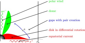
Figure 9. An electrospheric model for pulsars. Adapted from Pétri (Reference Pétri2002). The activity of this dead electrosphere could be revived by an equatorial current transporting charges across field lines due to non-neutral plasma instabilities and a polar wind made of charges of opposite sign to compensate for the equator loss of charges.
Table 6. The essential models describing the magnetosphere activity of a pulsar.
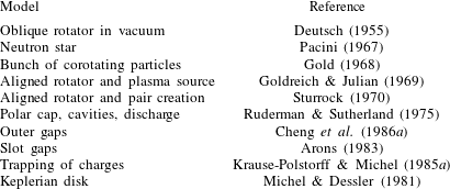
Table 7. The fundamental parameters of a normal and a millisecond pulsar.
7 Pulsar winds
It is often assumed that pulsars lose their rotational kinetic energy through the formation of an ultra-relativistic and magnetized wind, made essentially of leptonic
 $e^{\pm }$
pairs, and not just magnetodipole losses in vacuum which would contradict broadband pulsed emission. This energy, drawn from the rotational kinetic energy of the central star, is extracted via the Lorentz force exerted at the stellar crust
$e^{\pm }$
pairs, and not just magnetodipole losses in vacuum which would contradict broadband pulsed emission. This energy, drawn from the rotational kinetic energy of the central star, is extracted via the Lorentz force exerted at the stellar crust
 $\iint \boldsymbol{i}_{s}\wedge \boldsymbol{B}\,\text{d}S$
and carried away in an electromagnetic wave: the Poynting flux where
$\iint \boldsymbol{i}_{s}\wedge \boldsymbol{B}\,\text{d}S$
and carried away in an electromagnetic wave: the Poynting flux where
 $\boldsymbol{i}_{s}$
is the surface charge current and
$\boldsymbol{i}_{s}$
is the surface charge current and
 $\text{d}S$
the surface element. If surface charges are present, the electric force also contributes to the spin-down in the form
$\text{d}S$
the surface element. If surface charges are present, the electric force also contributes to the spin-down in the form
 $\iint \unicode[STIX]{x1D70E}_{e}[\boldsymbol{E}]\,\text{d}S$
where
$\iint \unicode[STIX]{x1D70E}_{e}[\boldsymbol{E}]\,\text{d}S$
where
 $\unicode[STIX]{x1D70E}_{e}$
is the surface electric charge and
$\unicode[STIX]{x1D70E}_{e}$
is the surface electric charge and
 $[\boldsymbol{E}]$
the jump in electric field across the same surface. Schematically, from an electrical point of view, the system generates a potential drop, the magnetized star delivering a potential difference equal to that between the centre and the rim of a polar cap, electric wires are replaced by open magnetic field lines and the resistive charge by the nebula acting as a calorimeter. The wind expands from the external parts of the pulsar magnetosphere, through the vicinity of the light cylinder, up to the neighbouring nebula and feed it with freshly made ultra-relativistic particles. Evolving in a magnetic field, these particles emit synchrotron and inverse Compton radiation, detectable as for instance in the famous Crab nebulaFootnote
6
. As a general picture, magnetized ultra-relativistic winds are thought to find their source in a compact object, neutron star or black hole. The flow, dominated by the Poynting flux, helps in the modelling of some quasars and gamma-ray bursts also (Blandford Reference Blandford, Gilfanov, Sunyaev and Churazov2002).
$[\boldsymbol{E}]$
the jump in electric field across the same surface. Schematically, from an electrical point of view, the system generates a potential drop, the magnetized star delivering a potential difference equal to that between the centre and the rim of a polar cap, electric wires are replaced by open magnetic field lines and the resistive charge by the nebula acting as a calorimeter. The wind expands from the external parts of the pulsar magnetosphere, through the vicinity of the light cylinder, up to the neighbouring nebula and feed it with freshly made ultra-relativistic particles. Evolving in a magnetic field, these particles emit synchrotron and inverse Compton radiation, detectable as for instance in the famous Crab nebulaFootnote
6
. As a general picture, magnetized ultra-relativistic winds are thought to find their source in a compact object, neutron star or black hole. The flow, dominated by the Poynting flux, helps in the modelling of some quasars and gamma-ray bursts also (Blandford Reference Blandford, Gilfanov, Sunyaev and Churazov2002).
7.1 Introduction
A pulsars radio luminosity only represents a tiny portion of its total energy losses, of the order of
 $10^{-5}L_{rot}$
. It is therefore believed that the major part of its rotational kinetic energy is expelled through a relativistic charged particle outflow: the pulsar wind. This fact is confirmed by observations showing the interaction between this wind and its surrounding nebula. In such picture, the luminosity of the Crab nebula is explained by synchrotron radiation of ultra-relativistic electrons emanating from the central neutron star.
$10^{-5}L_{rot}$
. It is therefore believed that the major part of its rotational kinetic energy is expelled through a relativistic charged particle outflow: the pulsar wind. This fact is confirmed by observations showing the interaction between this wind and its surrounding nebula. In such picture, the luminosity of the Crab nebula is explained by synchrotron radiation of ultra-relativistic electrons emanating from the central neutron star.
The problem of pulsar wind theory consists in elaborating a mechanism susceptible to converting the Poynting flux of the large-amplitude low-frequency strong electromagnetic wave into particle kinetic energy, as well as an acceleration process for these latter. By large amplitude we mean an electron gyro-frequency
 $\unicode[STIX]{x1D708}_{B}$
much greater than the wave frequency
$\unicode[STIX]{x1D708}_{B}$
much greater than the wave frequency
 $\unicode[STIX]{x1D708}$
, in other words
$\unicode[STIX]{x1D708}$
, in other words
 $\unicode[STIX]{x1D708}_{B}\gg \unicode[STIX]{x1D708}$
. For a pulsar, typical parameters are
$\unicode[STIX]{x1D708}_{B}\gg \unicode[STIX]{x1D708}$
. For a pulsar, typical parameters are
 $\unicode[STIX]{x1D708}\approx 0.1{-}720$
Hz and
$\unicode[STIX]{x1D708}\approx 0.1{-}720$
Hz and
 $\unicode[STIX]{x1D708}_{B}\gtrsim 10^{7}$
Hz.
$\unicode[STIX]{x1D708}_{B}\gtrsim 10^{7}$
Hz.
The links between the central pulsar, the supernova remnant and the nebula are well established. Let us recall the bottom line of this model, figure 10. At the source, in the centre of the nebula, the pulsar and its magnetosphere generates ultra-relativistic pairs
 $e^{\pm }$
. From faraway regions of the magnetosphere a cold ultra-relativistic wind forms and flows out towards the nebula, in a ballistic motion, that is a free expansion up to the termination shock (this latter being usually modelled in the ideal MHD regime) where particles are heated after crossing the shock to produce the shocked wind, in blue. This shocked wind is the main source of radiation observed in radio, optical, X-rays and gamma rays. The nebula is surrounded by the supernova remnant, in grey, itself imprisoned by the interstellar medium, in yellow. The transition between the unshocked and the shocked wind goes through the termination shock. The pre- and post-shock flow properties are radically different from a thermodynamic, but also from a radiative, point of view (particle distribution function, power-law index).
$e^{\pm }$
. From faraway regions of the magnetosphere a cold ultra-relativistic wind forms and flows out towards the nebula, in a ballistic motion, that is a free expansion up to the termination shock (this latter being usually modelled in the ideal MHD regime) where particles are heated after crossing the shock to produce the shocked wind, in blue. This shocked wind is the main source of radiation observed in radio, optical, X-rays and gamma rays. The nebula is surrounded by the supernova remnant, in grey, itself imprisoned by the interstellar medium, in yellow. The transition between the unshocked and the shocked wind goes through the termination shock. The pre- and post-shock flow properties are radically different from a thermodynamic, but also from a radiative, point of view (particle distribution function, power-law index).
Figure 10. Link between the pulsar and its surrounding nebula. In red, the pulsar and its magnetosphere, the source of
 $e^{\pm }$
pairs, in green, the wind in free, almost ballistic, expansion with a Lorentz factor
$e^{\pm }$
pairs, in green, the wind in free, almost ballistic, expansion with a Lorentz factor
 $\unicode[STIX]{x1D6E4}_{v}$
, in blue the shocked wind, in grey the supernova remnant and in yellow the interstellar medium. The termination shock is the boundary between the shocked (green) and unshocked (blue) wind.
$\unicode[STIX]{x1D6E4}_{v}$
, in blue the shocked wind, in grey the supernova remnant and in yellow the interstellar medium. The termination shock is the boundary between the shocked (green) and unshocked (blue) wind.
7.2 Basic theory
It is good to note that the exact nature of the pulsar wind remains mysterious, even basic properties such as its composition (leptonic plus a fraction of baryonic matter?) are unknown. We quickly come up against conceptual difficulties. However, pulsar winds fall essentially into three kinds of description ordered in a decreasing plasma particle density manner as follows
-
(i) A quasi-neutral wind of relativistic particles, usually described by the relativistic MHD formalism. This is the usual sense given to the notion of a wind. The electric current is arbitrary because it is generated by the relative velocity between different species of opposite charge. It requires a large particle density number.
-
(ii) A relativistic charged wind. Here intervenes an additional complication on account of the charge separation between particles of opposite sign. The electric current is no more arbitrary but explicitly linked to the velocity of the flow and to the charge density, it is only a convective current. It implies a low particle density number.
-
(iii) A large-amplitude low-frequency electromagnetic wave propagating into a low density plasma, particles surf on this wave with negligible back reaction of the plasma onto this wave. The electric current does not induce perceptible perturbations on this wave.
It is impossible to state which of these outflows prevail in a pulsar wind but it is believed that the wind cannot switch from one regime to another during its propagation towards the termination shock. The formation process of this wind in the vicinity of the neutron star, its propagation as well as its interaction with the nebula are still controversial. Theoretical investigations on pulsar winds mainly focus on propagation effects, little being known about their generation and repercussions on the nebula. The formation of the wind is the worse understood part of the pulsar.
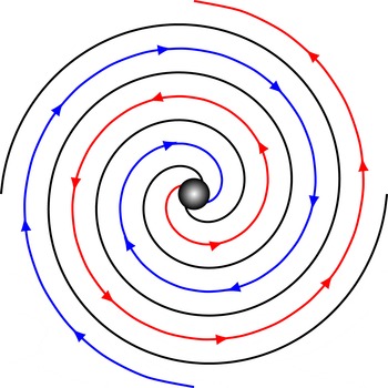
Figure 11. The Parker spiral structure of the solar wind. Outgoing field lines are shown in red, ingoing field lines in blue. The two black spirals correspond to places where magnetic polarity reverses. The same applies for the pulsar striped wind, see below.
7.3 Magnetohydrodynamic models
The modelling of pulsar winds goes back to the late 1960s. Indeed, the first model of a relativistic wind from a compact object was proposed by Michel (Reference Michel1969) as an extension of the solar wind theory exposed by Dicke (Reference Dicke1964), Modisette (Reference Modisette1967) and Weber & Davis (Reference Weber and Davis1967). The solar wind is a non-relativistic flow described by a fluid dominated by the pressure and not by the magnetic field. In the relativistic wind model, the magnetic field is monopolar, field lines are radial and symmetric with respect to the stellar rotation axis. Contrary to the solar wind, pressure as well as gravity were ignored. Because of the pulsar rotation, field lines roll up forming a spiral very similar to the Parker spiral (Parker Reference Parker1958). This structure will be met later again when explaining the pulsar striped wind model, figure 11. Particles, required to move along these lines, are then accelerated by catapult effect. In all these computations, the dimensionless quantity, sometimes called magnetization
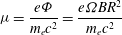 $$\begin{eqnarray}\displaystyle \unicode[STIX]{x1D707}=\frac{e\unicode[STIX]{x1D6F7}}{m_{e}c^{2}}=\frac{e\unicode[STIX]{x1D6FA}BR^{2}}{m_{e}c^{2}} & & \displaystyle\end{eqnarray}$$
introduced by Michel (Reference Michel1969) plays a significant role where
 $\unicode[STIX]{x1D6F7}$
is the electric potential drop. Physically, this parameter can be interpreted as the maximal Lorentz factor reached by particles when considering that all the Poynting flux goes into the kinetic energy of the particles. From an electrostatic point of view,
$\unicode[STIX]{x1D6F7}$
is the electric potential drop. Physically, this parameter can be interpreted as the maximal Lorentz factor reached by particles when considering that all the Poynting flux goes into the kinetic energy of the particles. From an electrostatic point of view,
 $\unicode[STIX]{x1D6F7}$
is the maximum potential drop between the magnetic poles and the equator for an aligned rotator
$\unicode[STIX]{x1D6F7}$
is the maximum potential drop between the magnetic poles and the equator for an aligned rotator
 $\unicode[STIX]{x1D6F7}=\unicode[STIX]{x1D6FA}BR^{2}$
. A probably less optimistic but better estimate of this electric potential drop is to take it along the polar cap from the centre to the rim such that
$\unicode[STIX]{x1D6F7}=\unicode[STIX]{x1D6FA}BR^{2}$
. A probably less optimistic but better estimate of this electric potential drop is to take it along the polar cap from the centre to the rim such that
 $\unicode[STIX]{x1D6F7}=\unicode[STIX]{x1D6FA}^{2}BR^{3}/c$
. However, previous studies have shown that the Lorentz factor related to this flow velocity of the wind is relatively low, the asymptotic Lorentz factor being only approximately
$\unicode[STIX]{x1D6F7}=\unicode[STIX]{x1D6FA}^{2}BR^{3}/c$
. However, previous studies have shown that the Lorentz factor related to this flow velocity of the wind is relatively low, the asymptotic Lorentz factor being only approximately
 $\unicode[STIX]{x1D707}^{1/3}$
. In a space-charge limited flow, acceleration can reach Lorentz factor of the order
$\unicode[STIX]{x1D707}^{1/3}$
. In a space-charge limited flow, acceleration can reach Lorentz factor of the order
 $\unicode[STIX]{x1D707}^{1/2}$
(Michel Reference Michel1974a
). This upper limit reaches
$\unicode[STIX]{x1D707}^{1/2}$
(Michel Reference Michel1974a
). This upper limit reaches
 $\unicode[STIX]{x1D707}^{2/3}$
for a charge separated wind (Michel Reference Michel1984). A summary is presented in table 8. Test particle acceleration has also been postulated or computed by several authors. For instance Goldreich & Julian (Reference Goldreich and Julian1969) claimed that the maximal Lorentz factor looks like
$\unicode[STIX]{x1D707}^{2/3}$
for a charge separated wind (Michel Reference Michel1984). A summary is presented in table 8. Test particle acceleration has also been postulated or computed by several authors. For instance Goldreich & Julian (Reference Goldreich and Julian1969) claimed that the maximal Lorentz factor looks like
 $\unicode[STIX]{x1D6FE}_{max}\approx \unicode[STIX]{x1D707}^{1/3}$
. On the other hand, Ostriker & Gunn (Reference Ostriker and Gunn1969) gave
$\unicode[STIX]{x1D6FE}_{max}\approx \unicode[STIX]{x1D707}^{1/3}$
. On the other hand, Ostriker & Gunn (Reference Ostriker and Gunn1969) gave
 $\unicode[STIX]{x1D6FE}_{max}\approx (\unicode[STIX]{x1D707}(1-r_{0}/r))^{2/3}$
. Buckley (Reference Buckley1977) claimed a linear acceleration with distance such that
$\unicode[STIX]{x1D6FE}_{max}\approx (\unicode[STIX]{x1D707}(1-r_{0}/r))^{2/3}$
. Buckley (Reference Buckley1977) claimed a linear acceleration with distance such that
 $\unicode[STIX]{x1D6FE}_{max}\approx r$
. Kennel, Schmidt & Wilcox (Reference Kennel, Schmidt and Wilcox1973) found
$\unicode[STIX]{x1D6FE}_{max}\approx r$
. Kennel, Schmidt & Wilcox (Reference Kennel, Schmidt and Wilcox1973) found
 $\unicode[STIX]{x1D6FE}_{max}\approx \unicode[STIX]{x1D707}$
.
$\unicode[STIX]{x1D6FE}_{max}\approx \unicode[STIX]{x1D707}$
.
Table 8. Asymptotic Lorentz factor reached according to three plasma regimes in the wind.
Starting from the hypothesis formulated by Michel (Reference Michel1969), Goldreich & Julian (Reference Goldreich and Julian1970) have added a pressure term as well as the gravitational field of the star. Solving the mass, energy and momentum conservation equations, they obtained an algebraic system. They showed that the flow passes through three critical points that are the sonic point where the velocity of the flow reaches the sound speed, the Alfvénic point and the magnetosonic point. In addition Henriksen & Rayburn (Reference Henriksen and Rayburn1971) computed the relativistic breeze solution complementary to Michel (Reference Michel1969). The magnetosonic point must however lie at a finite distance according to Ardavan (Reference Ardavan1979).
Rees & Gunn (Reference Rees and Gunn1974) were the first to look for a model of the spatial plasma distribution in the Crab nebula adopting a purely hydrodynamic point of view and assuming spherical symmetry. All the energy coming from the pulsar accumulates in the volume of the nebula which expands at a speed
 $v_{neb}\ll c$
. At a distance
$v_{neb}\ll c$
. At a distance
 $R_{s}$
, the total pressure in the nebula compensates the wind dynamical pressure. In a stationary regime
$R_{s}$
, the total pressure in the nebula compensates the wind dynamical pressure. In a stationary regime
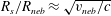 $R_{s}/R_{neb}\approx \sqrt{v_{neb}/c}$
, where
$R_{s}/R_{neb}\approx \sqrt{v_{neb}/c}$
, where
 $R_{neb}$
is the radius of the spherically symmetric nebula. Applied to the Crab nebula, the ratio is of the order 7 %. In this region a shock forms to make the transition from an ultra-relativistic wind down to a velocity of the order of
$R_{neb}$
is the radius of the spherically symmetric nebula. Applied to the Crab nebula, the ratio is of the order 7 %. In this region a shock forms to make the transition from an ultra-relativistic wind down to a velocity of the order of
 $c/\sqrt{3}$
Footnote
7
. Farther away from
$c/\sqrt{3}$
Footnote
7
. Farther away from
 $R_{s}$
, the flow becomes subsonic. The pressure will approximatively be uniform in the volume between the shock zone and the envelope of the nebula,
$R_{s}$
, the flow becomes subsonic. The pressure will approximatively be uniform in the volume between the shock zone and the envelope of the nebula,
 $R_{s}<r<R_{neb}$
. The wind passes therefore from a velocity
$R_{s}<r<R_{neb}$
. The wind passes therefore from a velocity
 $c/\sqrt{3}$
at
$c/\sqrt{3}$
at
 $R_{s}$
to a velocity
$R_{s}$
to a velocity
 $v_{neb}$
at
$v_{neb}$
at
 $R_{neb}$
. The absence of optical radiation in the centre of the Crab nebula for
$R_{neb}$
. The absence of optical radiation in the centre of the Crab nebula for
 $r<R_{s}$
was identified with a wind zone which is rather cold, underluminous and close to the pulsar.
$r<R_{s}$
was identified with a wind zone which is rather cold, underluminous and close to the pulsar.
Starting from the model of Rees & Gunn (Reference Rees and Gunn1974), Kennel & Coroniti (Reference Kennel and Coroniti1984a
) studied the details of the MHD shock of the nebula including the magnetic field dynamics with application to the Crab (Kennel & Coroniti Reference Kennel and Coroniti1984b
). Emmering & Chevalier (Reference Emmering and Chevalier1987) extended the previous solution to a time-dependent moving shock solution. To satisfy the boundary conditions at the supernova remnant (velocity and pressure), the wind must terminate by a MHD shock which is essentially hydrodynamic in nature, that is a flow dominated by particle pressure. They adopted a different definition of the magnetization compared to Michel (Reference Michel1969) and denoted by
 $\unicode[STIX]{x1D70E}$
, ratio between the electromagnetic energy flux and the particle energy flux. Its dynamics is still dominated by the Poynting flux symbolised by the magnetization parameter
$\unicode[STIX]{x1D70E}$
, ratio between the electromagnetic energy flux and the particle energy flux. Its dynamics is still dominated by the Poynting flux symbolised by the magnetization parameter
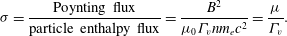 $$\begin{eqnarray}\displaystyle \unicode[STIX]{x1D70E}=\frac{\text{Poynting flux}}{\text{particle enthalpy flux}}=\frac{B^{2}}{\unicode[STIX]{x1D707}_{0}\unicode[STIX]{x1D6E4}_{v}nm_{e}c^{2}}=\frac{\unicode[STIX]{x1D707}}{\unicode[STIX]{x1D6E4}_{v}}. & & \displaystyle\end{eqnarray}$$
This definition is commonly used today, contrary to that of Michel with the parameter
 $\unicode[STIX]{x1D707}$
, which appears to be obsolete. Kennel & Coroniti (Reference Kennel and Coroniti1984b
) reproduced the optical and X-ray emission of the nebula assuming a cold wind hitting the termination shock with a Lorentz factor of
$\unicode[STIX]{x1D707}$
, which appears to be obsolete. Kennel & Coroniti (Reference Kennel and Coroniti1984b
) reproduced the optical and X-ray emission of the nebula assuming a cold wind hitting the termination shock with a Lorentz factor of
 $\unicode[STIX]{x1D6E4}_{v}\approx 10^{6}$
. Moreover, they showed that the magnetization should be of the order
$\unicode[STIX]{x1D6E4}_{v}\approx 10^{6}$
. Moreover, they showed that the magnetization should be of the order
 $\unicode[STIX]{x1D70E}\approx 10^{-3}$
, in other words, the relativistic wind emanating from the pulsar should be very dense and weakly magnetised. A copious production of
$\unicode[STIX]{x1D70E}\approx 10^{-3}$
, in other words, the relativistic wind emanating from the pulsar should be very dense and weakly magnetised. A copious production of
 $e^{+}e^{-}$
pairs in the magnetosphere could explain this high plasma density, solving simultaneously the shock problem that would then only be a Poynting dominated flow. In this model, the wind magnetic field is assumed to be essentially azimuthal, only the toroidal component
$e^{+}e^{-}$
pairs in the magnetosphere could explain this high plasma density, solving simultaneously the shock problem that would then only be a Poynting dominated flow. In this model, the wind magnetic field is assumed to be essentially azimuthal, only the toroidal component
 $B_{\unicode[STIX]{x1D711}}$
remaining non-negligible. Moreover, for the aligned rotator, the field keeps a unidirectional structure, that is, field lines cross the equatorial plane always in the same sense. See also Kundt & Krotscheck (Reference Kundt and Krotscheck1980) for a refinement of the Rees & Gunn (Reference Rees and Gunn1974) early model and details about geometrical, spectral and temporal features of the Crab nebula.
$B_{\unicode[STIX]{x1D711}}$
remaining non-negligible. Moreover, for the aligned rotator, the field keeps a unidirectional structure, that is, field lines cross the equatorial plane always in the same sense. See also Kundt & Krotscheck (Reference Kundt and Krotscheck1980) for a refinement of the Rees & Gunn (Reference Rees and Gunn1974) early model and details about geometrical, spectral and temporal features of the Crab nebula.
Begelman & Li (Reference Begelman and Li1994) studied the conversion of Poynting flux into particle kinetic energy for radial and axisymmetric flow. Under such hypotheses, they showed that plasma acceleration was extremely inefficient because of magnetic pressure cancellation by magnetic tension. But if the flow could deviate from this radial motion even slightly, it would become magnetosonic and induce a significant acceleration. Unfortunately, the magnetization parameter
 $\unicode[STIX]{x1D70E}$
decreases only logarithmically with the radius, which is not sufficient to explain observations of the Crab nebula. Inefficient acceleration is counterbalanced by the finite temperature of the wind, as shown by Kennel, Fujimura & Okamoto (Reference Kennel, Fujimura and Okamoto1983) but synchrotron emission quickly cools particles. Therefore, there is no simple and satisfactory explanation to the wind acceleration up to the termination shock. Chiueh, Li & Begelman (Reference Chiueh, Li and Begelman1998) showed that it is impossible to transfer electromagnetic energy flux to particles in a relativistic stationary MHD flow. Only a gradual acceleration can occur and therefore
$\unicode[STIX]{x1D70E}$
decreases only logarithmically with the radius, which is not sufficient to explain observations of the Crab nebula. Inefficient acceleration is counterbalanced by the finite temperature of the wind, as shown by Kennel, Fujimura & Okamoto (Reference Kennel, Fujimura and Okamoto1983) but synchrotron emission quickly cools particles. Therefore, there is no simple and satisfactory explanation to the wind acceleration up to the termination shock. Chiueh, Li & Begelman (Reference Chiueh, Li and Begelman1998) showed that it is impossible to transfer electromagnetic energy flux to particles in a relativistic stationary MHD flow. Only a gradual acceleration can occur and therefore
 $\unicode[STIX]{x1D70E}$
remains high before the termination shock, which agrees with the conclusions of Begelman & Li (Reference Begelman and Li1994). An abrupt acceleration, not far from the light cylinder, should happen.
$\unicode[STIX]{x1D70E}$
remains high before the termination shock, which agrees with the conclusions of Begelman & Li (Reference Begelman and Li1994). An abrupt acceleration, not far from the light cylinder, should happen.
To summarize so far pulsar wind theory, a cold MHD flow in a stationary regime evolving in a monopole magnetic field is always dominated by the Poynting flux if particles are injected with
 $\unicode[STIX]{x1D70E}\gg 1$
, the flow reaching the magneto-sonic point asymptotically. However independent estimates from the Crab nebula furnish a value of the flow parameter less than 1,
$\unicode[STIX]{x1D70E}\gg 1$
, the flow reaching the magneto-sonic point asymptotically. However independent estimates from the Crab nebula furnish a value of the flow parameter less than 1,
 $\unicode[STIX]{x1D70E}\ll 1$
, a required condition for sufficient confinement pressure for keeping particles inside the supernova remnant. Numerous questions remain unsettled, as for instance to the precise description of the shock, the formation of a dense wind close to the pulsar surface, the nature of the large-amplitude electromagnetic wave, a wave in vacuum or a plasma wave, the current circulation and related MHD/kinetic instabilities.
$\unicode[STIX]{x1D70E}\ll 1$
, a required condition for sufficient confinement pressure for keeping particles inside the supernova remnant. Numerous questions remain unsettled, as for instance to the precise description of the shock, the formation of a dense wind close to the pulsar surface, the nature of the large-amplitude electromagnetic wave, a wave in vacuum or a plasma wave, the current circulation and related MHD/kinetic instabilities.
The above models are drastic simplifications of a real system because they assumed stationarity, no explicit time dependence is included. Indeed, the firsts models were presented by Rees & Gunn (Reference Rees and Gunn1974) for the Crab nebula and interpreted as synchrotron emission from the relativistic shocked wind in a spherical geometry with a more detailed study by Kennel & Coroniti (Reference Kennel and Coroniti1984a ,Reference Kennel and Coroniti b ) where they introduced an in-depth study of the relativistic MHD shock. The formulation relies on three hypotheses that are
-
(i) A Larmor radius smaller than the size of the nebula.
-
(ii) Negligible radiative losses, i.e. a cooling time much longer than the age of the nebula.
-
(iii) A plasma made almost exclusively of
$e^{\pm }$
pairs with little ions and/or heavy elements. There are therefore no time and length scales characteristics that differ because of the mass ratio.

But a pulsar and its wind are far from being stationary. The magnetic moment inclined with respect to the rotation axis generates a variable electromagnetic field that at the light cylinder gives rise to a large-amplitude low-frequency electromagnetic wave damped by its interaction with the surrounding plasma causing its dissipation.
Coroniti (Reference Coroniti1990) was the first to recognize the importance of the time dependence of the wind structure on the energy transport mechanism. He noted that for an oblique rotator, the azimuthal component of the magnetic field in the wind change polarity alternatively in the vicinity of the rotational equatorial planeFootnote
8
, the flux being equal in the two alternations. The wind, qualified as a striped wind, develops into a structure made of stripes that are alternating polarity from positive to negative and vice versa, separated by a neutral surface onto which the field vanishes: the current sheet. He demonstrated that magnetic field line annihilation of opposite polarity can result from an initial highly magnetized configuration, a flow dominated by the propagation of electromagnetic waves at
 $\unicode[STIX]{x1D70E}\gg 1$
, to a weakly magnetized wind, dominated by particle kinetic energy at
$\unicode[STIX]{x1D70E}\gg 1$
, to a weakly magnetized wind, dominated by particle kinetic energy at
 $\unicode[STIX]{x1D70E}\ll 1$
. This annihilation is also refereed to magnetic reconnection in the striped wind.
$\unicode[STIX]{x1D70E}\ll 1$
. This annihilation is also refereed to magnetic reconnection in the striped wind.
Michel (Reference Michel1994) interpreted this magnetic reconnection merely in terms of inductive heating because of the plasma short circuit necessary to maintain the current. The density of particles responsible for this electric current maintaining the striped structure decreases radially faster, like
 $n\propto 1/r^{2}$
, than the amplitude of the magnetic field, like
$n\propto 1/r^{2}$
, than the amplitude of the magnetic field, like
 $B\propto 1/r$
. However the Maxwell–Ampère equation imposes a radial decrease identical for both the density
$B\propto 1/r$
. However the Maxwell–Ampère equation imposes a radial decrease identical for both the density
 $n$
and magnetic field
$n$
and magnetic field
 $B$
leading to a contradiction. The difficulty is circumvented by draining the reservoir of cold and magnetized particles, making them join those that are hot and weakly magnetized. This source shrinks until exhaustion and dissipation of the field itself. More clearly, particles can no longer maintain the current and to insure the existence of the stripes that have no other choice than to dissipate. This problem between the charge density and the current density was already noted by Usov (Reference Usov1975).
$B$
leading to a contradiction. The difficulty is circumvented by draining the reservoir of cold and magnetized particles, making them join those that are hot and weakly magnetized. This source shrinks until exhaustion and dissipation of the field itself. More clearly, particles can no longer maintain the current and to insure the existence of the stripes that have no other choice than to dissipate. This problem between the charge density and the current density was already noted by Usov (Reference Usov1975).
The striped wind shows the peculiarity of alternating polarity in the magnetic field in the equatorial plane. An oscillating current sheet emerges out of this system and separates equatorial stripes (Bogovalov Reference Bogovalov1999). The striped wind is considered as an entropic wave, that is a wave moving with the bulk flow without entropy exchange between different parts of the fluid. Note that energy is mainly evacuated in the equatorial region. The dynamics of the striped wind is much more rich than that of a simple spherically symmetric radial wind. Indeed, Lyubarsky & Kirk (Reference Lyubarsky and Kirk2001) have shown that the thin current sheet represents a favourable site for magnetic field annihilation in the stripes. Magnetic energy is therefore transferred to particles via reconnection. But acceleration induced by this reconnection slows down the dissipation rate estimated by a distant observer because of time dilation, rendering this mechanism inefficient to completely dissipate the magnetic field before entering the termination shock. The Lorentz factor increases faster than logarithmically but not sufficiently, only as
 $\unicode[STIX]{x1D6E4}_{v}\propto \sqrt{r}$
. The conversion could however be possible in favourable conditions with a higher than expected density of pairs through cascading (Kirk & Skjæraasen Reference Kirk and Skjæraasen2003). This result contradicts the general belief stipulating a domination of particles over the electromagnetic field before passage through the termination shock. Indeed, a too high magnetization at the shock would drastically increase the post-shock pressure with as a consequence an important deformation of the nebula, which is not observed. The other hypothesis meets some difficulties in explaining the radio spectrum. An alternative solution consists in dissipating the magnetic field within the termination shock (Lyubarsky Reference Lyubarsky2005; Pétri & Lyubarsky Reference Pétri and Lyubarsky2007; Sironi & Spitkovsky Reference Sironi and Spitkovsky2011), which would solve the problem of a flow dominated by the Poynting flux and avoid that of the radio spectrum (Lyubarsky Reference Lyubarsky2003b
). Alternatively, wave dissipation in the striped wind has been studied by Lyubarsky (Reference Lyubarsky2003a
) who showed the decay of fast magnetosonic waves in such winds through nonlinear steepening and multiple shock formation. Superluminal waves offer another interesting point of view to dissipate efficiently electromagnetic energy at the termination shock (Arka & Kirk Reference Arka and Kirk2012).
$\unicode[STIX]{x1D6E4}_{v}\propto \sqrt{r}$
. The conversion could however be possible in favourable conditions with a higher than expected density of pairs through cascading (Kirk & Skjæraasen Reference Kirk and Skjæraasen2003). This result contradicts the general belief stipulating a domination of particles over the electromagnetic field before passage through the termination shock. Indeed, a too high magnetization at the shock would drastically increase the post-shock pressure with as a consequence an important deformation of the nebula, which is not observed. The other hypothesis meets some difficulties in explaining the radio spectrum. An alternative solution consists in dissipating the magnetic field within the termination shock (Lyubarsky Reference Lyubarsky2005; Pétri & Lyubarsky Reference Pétri and Lyubarsky2007; Sironi & Spitkovsky Reference Sironi and Spitkovsky2011), which would solve the problem of a flow dominated by the Poynting flux and avoid that of the radio spectrum (Lyubarsky Reference Lyubarsky2003b
). Alternatively, wave dissipation in the striped wind has been studied by Lyubarsky (Reference Lyubarsky2003a
) who showed the decay of fast magnetosonic waves in such winds through nonlinear steepening and multiple shock formation. Superluminal waves offer another interesting point of view to dissipate efficiently electromagnetic energy at the termination shock (Arka & Kirk Reference Arka and Kirk2012).
In all these scenarios, whatever the situation considered, after dissipation, the alternating component of the magnetic field disappears and only the DC component subsists, obtained by averaging of the magnetic field on a wavelength of the wind. In the equatorial plane, this mean value is strictly null. However, in polar regions, the same magnetic field does not change polarity, there are no stripes to annihilate. Energy is transported via magneto-sonic waves or Alfvén waves. In the asymptotic region, field lines tend to the split monopole (Ingraham Reference Ingraham1973; Michel Reference Michel1974b ). Buckley (Reference Buckley1977) showed that any solution possesses a neutral current sheet, that the asymptotic solution resembles a wave in vacuum and that the particle Lorentz factor increases approximatively linearly with the distance. The flow remains essentially radial after crossing the magneto-sonic point because collimation becomes inefficient (Beskin, Kuznetsova & Rafikov Reference Beskin, Kuznetsova and Rafikov1998; Chiueh et al. Reference Chiueh, Li and Begelman1998; Tomimatsu Reference Tomimatsu1994). We know since the works of Asseo, Kennel & Pellat (Reference Asseo, Kennel and Pellat1978) that low-frequency waves generated by the pulsar rotation are heavily damped due to the presence of a dense plasma.
The MHD model alone, as we see, cannot explain individual acceleration of particles as power-law distributions but rather as simple Maxwellians in a hypothetical thermal equilibrium state. Although the wind properties are not directly accessible to observation, an indirect deduction of the magnetization, of the angular distribution of energy and of the dissipation in the equatorial plane can be gained from numerical simulations.
7.4 Axisymmetric magnetohydrodynamical simulations
With the advent of relativistic numerical codes noteworthy progress has been made in the comprehension of the geometry of pulsar wind nebulae. For instance, relativistic magnetohydrodynamic simulations (RMHD) performed by Komissarov & Lyubarsky (Reference Komissarov and Lyubarsky2004) have shown that the jet+torus structure, well resolved in the Crab nebula, can be explained by a relativistic wind possessing a weak magnetization at the equator
 $\unicode[STIX]{x1D70E}\ll 1$
but an important Poynting flux. The transition to the nebula goes through an anisotropic termination shock braking the wind to a velocity of approximately
$\unicode[STIX]{x1D70E}\ll 1$
but an important Poynting flux. The transition to the nebula goes through an anisotropic termination shock braking the wind to a velocity of approximately
 $c/2$
. Jets are formed after this shock by magnetic confinement. Moreover, synchrotron emission resulting from such a configuration reproduces faithfully X-ray observations of the Crab nebula. The rings are easily identifiable with the symmetrical jets seeming to escape from the pulsar. Since their work, numerous other simulations have reproduced similar results, see for instance Del Zanna, Amato & Bucciantini (Reference Del Zanna, Amato and Bucciantini2004), Bucciantini et al. (Reference Bucciantini, Thompson, Arons, Quataert and Del Zanna2006), Del Zanna et al. (Reference Del Zanna, Volpi, Amato and Bucciantini2006) and Volpi et al. (Reference Volpi, Del Zanna, Amato and Bucciantini2008).
$c/2$
. Jets are formed after this shock by magnetic confinement. Moreover, synchrotron emission resulting from such a configuration reproduces faithfully X-ray observations of the Crab nebula. The rings are easily identifiable with the symmetrical jets seeming to escape from the pulsar. Since their work, numerous other simulations have reproduced similar results, see for instance Del Zanna, Amato & Bucciantini (Reference Del Zanna, Amato and Bucciantini2004), Bucciantini et al. (Reference Bucciantini, Thompson, Arons, Quataert and Del Zanna2006), Del Zanna et al. (Reference Del Zanna, Volpi, Amato and Bucciantini2006) and Volpi et al. (Reference Volpi, Del Zanna, Amato and Bucciantini2008).
The crucial point in these relativistic MHD simulations is the presence of an anisotropy in the Poynting flux given by a prescription in luminosity according to the formal latitude dependence (Lyubarsky Reference Lyubarsky2002)
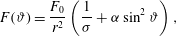 $$\begin{eqnarray}\displaystyle F(\unicode[STIX]{x1D717})=\frac{F_{0}}{r^{2}}\left(\frac{1}{\unicode[STIX]{x1D70E}}+\unicode[STIX]{x1D6FC}\sin ^{2}\unicode[STIX]{x1D717}\right), & & \displaystyle\end{eqnarray}$$
where
 $F_{0}$
and
$F_{0}$
and
 $1/\unicode[STIX]{x1D70E}$
are two constant parameters. The first term accounts for particle energy and the second for the Poynting flux reminiscent of the striped wind. The weak magnetization in the equator is accounted for by magnetic dissipation in the stripes. It seems to be the most accomplished model to explain the jet+torus structure of nebulas. The plasma flow is facilitated in the equatorial plane with a magnetic compression along the axis, thus forming the jet. The formation of this jet depends on the magnetization upstream the wind. For a weak value of
$1/\unicode[STIX]{x1D70E}$
are two constant parameters. The first term accounts for particle energy and the second for the Poynting flux reminiscent of the striped wind. The weak magnetization in the equator is accounted for by magnetic dissipation in the stripes. It seems to be the most accomplished model to explain the jet+torus structure of nebulas. The plasma flow is facilitated in the equatorial plane with a magnetic compression along the axis, thus forming the jet. The formation of this jet depends on the magnetization upstream the wind. For a weak value of
 $\unicode[STIX]{x1D70E}$
, let us say
$\unicode[STIX]{x1D70E}$
, let us say
 $\unicode[STIX]{x1D70E}<10^{-3}$
, there is no jet but for
$\unicode[STIX]{x1D70E}<10^{-3}$
, there is no jet but for
 $\unicode[STIX]{x1D70E}\approx 0.1$
a jet appears with an ejection velocity of approximately 0.7
$\unicode[STIX]{x1D70E}\approx 0.1$
a jet appears with an ejection velocity of approximately 0.7
 $c$
. Stripes add to the complexity of the flow in the nebula because they can dissipate and lower the equatorial magnetization. This is necessary to explain the inner ring and the external torus. Should the opposite occur, a constant magnetization would be impossible. The intensity of the magnetic field increases by MHD compression of the wind in the shock (Piddington Reference Piddington1969; Pacini & Salvati Reference Pacini and Salvati1973; Rees & Gunn Reference Rees and Gunn1974). Two-dimensional axisymmetric RMHD of Komissarov & Lyubarsky (Reference Komissarov and Lyubarsky2004) have confirmed the veracity of these hypotheses. Their conclusions are the following
$c$
. Stripes add to the complexity of the flow in the nebula because they can dissipate and lower the equatorial magnetization. This is necessary to explain the inner ring and the external torus. Should the opposite occur, a constant magnetization would be impossible. The intensity of the magnetic field increases by MHD compression of the wind in the shock (Piddington Reference Piddington1969; Pacini & Salvati Reference Pacini and Salvati1973; Rees & Gunn Reference Rees and Gunn1974). Two-dimensional axisymmetric RMHD of Komissarov & Lyubarsky (Reference Komissarov and Lyubarsky2004) have confirmed the veracity of these hypotheses. Their conclusions are the following
-
(i) At high latitude, the magnetic field is still significant, inducing a jet collimation.
-
(ii) The termination shock is closer to the neutron star at the poles than at the equator.
The a posteriori treatment of simulation data to extract synchrotron intensity maps should convince the most sceptical.
To conclude regarding simulations, Porth, Komissarov & Keppens (Reference Porth, Komissarov and Keppens2014) reported on the first full 3-D relativistic MHD simulations of a pulsar wind nebula. They showed that observations can be reconciled with theory even with magnetization as high as
 $\unicode[STIX]{x1D70E}=3$
thanks to a kink instability occurring in the polar regions, as already mentioned by Begelman (Reference Begelman1998).
$\unicode[STIX]{x1D70E}=3$
thanks to a kink instability occurring in the polar regions, as already mentioned by Begelman (Reference Begelman1998).
7.5 Wind observability
The striped wind being a cold flow, at first sight it seems difficult to observe it even indirectly. However, some regions in the wind are detectable whereas other should remain invisible for observers on Earth. On one hand, the unshocked part of the wind, essentially cold but made of a thin hot stripe (usually also assimilated to the current sheet), generates high- and very-high-energy photons through essentially two main channels, namely
-
(i) Inverse Compton emission on target photons emanating from
-
(a) The cosmic microwave background.
-
(b) Synchrotron photons (then called synchrotron self-Compton emission).
-
(c) Thermal photons from the stellar surface (heated to X-rays and thus energies of approximately 100 eV) (Bogovalov & Aharonian Reference Bogovalov and Aharonian2000).
-
(d) Optical/UV photons (typical energies of approximately several eV) from the companion in a binary system (Ball & Kirk Reference Ball and Kirk2000).
-
(e) Infrared dust.
-
(f) The surrounding nebula.
-
-
(ii) Synchrotron emission in the dense and hot stripes and incidentally in the cold and magnetized part with prediction of the associated polarisation.
Pulses are observable from optical up to MeV/GeV outside the magnetosphere but close to the light cylinder where emissivity is the highest. The pulsation observability condition is constrained by relativistic beaming, retardation and geometrical effects. If emission occurs at a radius
 $r$
and within a range
$r$
and within a range
 $\unicode[STIX]{x0394}r$
then according to Kirk, Skjæraasen & Gallant (Reference Kirk, Skjæraasen and Gallant2002) and Pétri (Reference Pétri2009a
, Reference Pétri2011) pulses are restricted to regions where
$\unicode[STIX]{x0394}r$
then according to Kirk, Skjæraasen & Gallant (Reference Kirk, Skjæraasen and Gallant2002) and Pétri (Reference Pétri2009a
, Reference Pétri2011) pulses are restricted to regions where
 $$\begin{eqnarray}\displaystyle \{r,\unicode[STIX]{x0394}r\}\lesssim \unicode[STIX]{x1D6E4}_{v}^{2}r_{L}. & & \displaystyle\end{eqnarray}$$
On the other hand, the shocked part of the wind does not contain any stripes, they have been destroyed during the passage through the termination shock. In some special regimes of the plasma flow, stripes could survive as explained by Pétri & Lyubarsky (Reference Pétri and Lyubarsky2007). The magnetic field leaves room for very hot particles scattering photons up to TeV energies. There are nor pulses at these extreme energies but orbital phase modulation is expected, see for instance the case of PSR B1259-63 studied by Kirk, Ball & Skjaeraasen (Reference Kirk, Ball and Skjaeraasen1999) and Pétri & Dubus (Reference Pétri and Dubus2011).
Because radio emission must propagate through the wind to reach the observer at Earth, the wind needs to be transparent vis-à-vis inverse Compton scattering of radio photons. From this condition Wilson & Rees (Reference Wilson and Rees1978) deduced a minimum Lorentz factor of
 $\unicode[STIX]{x1D6E4}_{v}>10^{4}$
for the Crab at a distance of
$\unicode[STIX]{x1D6E4}_{v}>10^{4}$
for the Crab at a distance of
 $100r_{L}$
of the pulsar. Sincell & Krolik (Reference Sincell and Krolik1992) included ambient magnetic field effects altering the spectra and radio polarisation.
$100r_{L}$
of the pulsar. Sincell & Krolik (Reference Sincell and Krolik1992) included ambient magnetic field effects altering the spectra and radio polarisation.
We therefore conclude that the essentially cold wind is observable at least partly thanks to synchrotron and inverse Compton emission from the shocked and/or unshocked wind. The luminosity is indeed sufficient to be detectable on Earth. Moreover spectral and pulsation features differ from those of the nebula, the two components are therefore distinguishable.
8 The striped wind
In this paragraph, we discuss the possible observational signatures of the striped wind on the properties of high-energy emission induced by synchrotron and/or inverse Compton radiation of the current sheet containing ultra-relativistic electron–positron pairs. We focus more specifically on the pulsed component of this emission, beyond the optical domain, that is
 $E_{\unicode[STIX]{x1D6FE}}\gtrsim 1$
eVFootnote
9
. The striped wind being too rarely described in detail in the literature, an effort is made to give a precise and coherent description. Many of the striped wind emission features are based on the 3-D geometry of the underlying magnetic field. It imprints on the light-curve intensity as well as on polarisation. A more detailed model about kinetic aspects of the sheet interior would allow a survey of physical conditions within it, but the large span in time and spatial scales of many decades forbids a self-consistent treatment of global scales including microphysics.
$E_{\unicode[STIX]{x1D6FE}}\gtrsim 1$
eVFootnote
9
. The striped wind being too rarely described in detail in the literature, an effort is made to give a precise and coherent description. Many of the striped wind emission features are based on the 3-D geometry of the underlying magnetic field. It imprints on the light-curve intensity as well as on polarisation. A more detailed model about kinetic aspects of the sheet interior would allow a survey of physical conditions within it, but the large span in time and spatial scales of many decades forbids a self-consistent treatment of global scales including microphysics.
Pulsar nebulas are the natural results of the shocked plasma injected by the pulsar wind. This wind, although highly magnetized, is assumed to be cold, relatively homogeneous and does not radiate synchrotron photons, at most high-energy inverse Compton photons from scattering an exterior target field. This explains the lack of observation between the position of the neutron star and the inner parts of the nebula. Can we however hope to observe this wind even indirectly? We tempt to answer this question in the following lines.
8.1 Structure of the striped wind
A quantitatively accurate description of the striped wind is still not accessible. The main problems arise because of the very different time and length scales coming into play. On one hand, the global structure at large scales is dominated by the MHD regime and on the other hand the kinetic structure of the current sheet dominates at very small scales, both being difficult to reconcile from the point of view of numerical simulations. The Larmor radius is many orders of magnitude smaller than the wind wavelength. Radiation should also strongly influence the equilibrium configuration. Strong disparities in the time scale characteristics appears for instance in the three important frequencies namely the cyclotron frequency, the plasma frequency and the rotation frequency. See table 7 for a summary of important pulsar parameters.
Nevertheless, the magnetic field geometry at large distances in the MHD approximation is satisfactorily described by a split monopole. The use of such a structure avoids a detailed description of the closed pulsar magnetosphere. Indeed, the plasma configuration in the immediate surrounding of the neutron star, that is for distances less than the light-cylinder radius, remains largely unknown and ill understood. We only guess that a transition of the magnetic topology must occur approximatively at the light cylinder, switching from a confined corotating (or maybe differentially rotating) plasma to an open topology sustained by a wind of charged particles, the pulsar wind. Despite this large uncertainty, it is possible to get a simple analytical solution for the wind, independent of the precise knowledge of this magnetosphere. It is called the split monopole of which we recall some essential features.
8.2 The split monopole
Exact analytical solutions of the electromagnetic field around pulsars are sufficiently rare to be of interest from a purely physical point of view, even if assuming a monopolar magnetic structure is unrealistic. The split monopole model belongs to such rare solutions and has been introduced by Michel (Reference Michel1973b ). He started from the assumption that all the magnetic field lines at the surface of the star are radial and given by a monopole structure such that
 $$\begin{eqnarray}\displaystyle \boldsymbol{B}=B_{L}\frac{r_{L}^{2}}{r^{2}}\boldsymbol{e}_{r}, & & \displaystyle\end{eqnarray}$$
where
 $B_{L}$
is the magnetic field intensity at the light cylinder. He found an exact analytical solution of the pulsar (3.11), whose solution can be summarized in the formula below for the magnetic field
$B_{L}$
is the magnetic field intensity at the light cylinder. He found an exact analytical solution of the pulsar (3.11), whose solution can be summarized in the formula below for the magnetic field
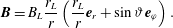 $$\begin{eqnarray}\displaystyle \boldsymbol{B}=B_{L}\frac{r_{L}}{r}\left(\frac{r_{L}}{r}\boldsymbol{e}_{r}+\sin \unicode[STIX]{x1D717}\boldsymbol{e}_{\unicode[STIX]{x1D711}}\right). & & \displaystyle\end{eqnarray}$$
The radial
 $B_{r}$
and toroidal
$B_{r}$
and toroidal
 $B_{\unicode[STIX]{x1D711}}$
components have same intensity at the light cylinder radius in the equatorial plane. The electric field possesses only a latitudinal component and is fully given by the expression
$B_{\unicode[STIX]{x1D711}}$
components have same intensity at the light cylinder radius in the equatorial plane. The electric field possesses only a latitudinal component and is fully given by the expression
 $E_{\unicode[STIX]{x1D717}}=cB_{\unicode[STIX]{x1D711}}$
. Particles undergo an electric drift motion combined with a movement along field lines such that the resulting velocity causes an ultra-relativistic outgoing flow (actually equal to the speed of light) with a purely radial component of the fluid such that
$E_{\unicode[STIX]{x1D717}}=cB_{\unicode[STIX]{x1D711}}$
. Particles undergo an electric drift motion combined with a movement along field lines such that the resulting velocity causes an ultra-relativistic outgoing flow (actually equal to the speed of light) with a purely radial component of the fluid such that
 $$\begin{eqnarray}\displaystyle \boldsymbol{V}=c\boldsymbol{e}_{r}. & & \displaystyle\end{eqnarray}$$
The radial component of the Poynting vector is easily derived to be
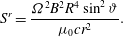 $$\begin{eqnarray}\displaystyle S^{r}=\frac{\unicode[STIX]{x1D6FA}^{2}B^{2}R^{4}\sin ^{2}\unicode[STIX]{x1D717}}{\unicode[STIX]{x1D707}_{0}cr^{2}}. & & \displaystyle\end{eqnarray}$$
We recognize the
 $\sin ^{2}\unicode[STIX]{x1D717}$
dependence used in the RMHD simulations of § 5. The Poynting vector in (8.4) leads to a total spin-down luminosity of
$\sin ^{2}\unicode[STIX]{x1D717}$
dependence used in the RMHD simulations of § 5. The Poynting vector in (8.4) leads to a total spin-down luminosity of
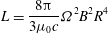 $$\begin{eqnarray}\displaystyle L=\frac{8\unicode[STIX]{x03C0}}{3\unicode[STIX]{x1D707}_{0}c}\unicode[STIX]{x1D6FA}^{2}B^{2}R^{4} & & \displaystyle\end{eqnarray}$$
and therefore a braking index equal to one,
 $n=1$
. Thus to summarize, for a monopole we get
$n=1$
. Thus to summarize, for a monopole we get
 $n=1$
and for a dipole
$n=1$
and for a dipole
 $n=3$
. In the most general case of a multipole of order
$n=3$
. In the most general case of a multipole of order
 $\ell$
we can estimate the Poynting flux by very general arguments in the following way. Approximately speaking, energy is taken away by the electromagnetic wave starting at the light cylinder
$\ell$
we can estimate the Poynting flux by very general arguments in the following way. Approximately speaking, energy is taken away by the electromagnetic wave starting at the light cylinder
 $r_{L}$
that is in the wave zone. The total energy flux across the sphere of radius
$r_{L}$
that is in the wave zone. The total energy flux across the sphere of radius
 $r_{L}$
is
$r_{L}$
is
 $4\unicode[STIX]{x03C0}B_{L}^{2}r_{L}^{2}c/\unicode[STIX]{x1D707}_{0}$
. For the multipole
$4\unicode[STIX]{x03C0}B_{L}^{2}r_{L}^{2}c/\unicode[STIX]{x1D707}_{0}$
. For the multipole
 $\ell$
the strength at the light cylinder
$\ell$
the strength at the light cylinder
 $B_{L}$
is connected to the strength at the surface
$B_{L}$
is connected to the strength at the surface
 $B$
by
$B$
by
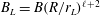 $B_{L}=B(R/r_{L})^{\ell +2}$
. Plugging into the energy flux we get
$B_{L}=B(R/r_{L})^{\ell +2}$
. Plugging into the energy flux we get
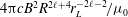 $4\unicode[STIX]{x03C0}cB^{2}R^{2\ell +4}r_{L}^{-2\ell -2}/\unicode[STIX]{x1D707}_{0}$
. Thus the Poynting flux is approximately
$4\unicode[STIX]{x03C0}cB^{2}R^{2\ell +4}r_{L}^{-2\ell -2}/\unicode[STIX]{x1D707}_{0}$
. Thus the Poynting flux is approximately
 $L\approx 4\unicode[STIX]{x03C0}B^{2}R^{2\ell +4}\unicode[STIX]{x1D6FA}^{2\ell +2}/\unicode[STIX]{x1D707}_{0}c^{2\ell +1}$
. We deduce the braking index to be
$L\approx 4\unicode[STIX]{x03C0}B^{2}R^{2\ell +4}\unicode[STIX]{x1D6FA}^{2\ell +2}/\unicode[STIX]{x1D707}_{0}c^{2\ell +1}$
. We deduce the braking index to be
 $n=2\ell +1$
as noted by Krolik (Reference Krolik1991). This estimate is valid irrespective of a vacuum or plasma assumption around the neutron star. A wind in the dipolar magnetosphere implies a braking index of
$n=2\ell +1$
as noted by Krolik (Reference Krolik1991). This estimate is valid irrespective of a vacuum or plasma assumption around the neutron star. A wind in the dipolar magnetosphere implies a braking index of
 $n=3$
in vacuum, in FFE and in general relatively (Pétri Reference Pétri2016a
). Most of the Poynting flux goes away along the equatorial plane with
$n=3$
in vacuum, in FFE and in general relatively (Pétri Reference Pétri2016a
). Most of the Poynting flux goes away along the equatorial plane with
 $S^{r}(\unicode[STIX]{x1D717})\propto \sin ^{2}\unicode[STIX]{x1D717}$
explaining the set-up for the RMHD simulations. The total magnetic flux through a sphere centred on the neutron star is not zero. To find a situation that meets the overall constraint of lack of magnetic monopole, the requirement is to reverse the direction of the magnetic field lines when changing hemisphere. Suppose that in the northern hemisphere field lines come out of the star. Conversely, in the southern hemisphere, field lines return to the star. By the symmetry of the problem, the total magnetic flux through a sphere centred on the star now vanishes. Moreover, this magnetic topology is an exact solution of the pulsar equation with a significant peculiarity. Indeed, the junction between both magnetic monopoles of opposite magnetic charge induces a discontinuity in the equatorial plane because its polarity changes sign. In order to satisfy the Maxwell–Ampère equation, this discontinuity must be maintained by a surface current density (the current sheet). For an aligned rotator, this surface coincides with the rotational equatorial plane of the neutron star, figure 12. A split monopole is constituted of two magnetic monopoles with equal but opposite magnetic charge between the northern and southern hemisphere. What about an oblique rotator?
$S^{r}(\unicode[STIX]{x1D717})\propto \sin ^{2}\unicode[STIX]{x1D717}$
explaining the set-up for the RMHD simulations. The total magnetic flux through a sphere centred on the neutron star is not zero. To find a situation that meets the overall constraint of lack of magnetic monopole, the requirement is to reverse the direction of the magnetic field lines when changing hemisphere. Suppose that in the northern hemisphere field lines come out of the star. Conversely, in the southern hemisphere, field lines return to the star. By the symmetry of the problem, the total magnetic flux through a sphere centred on the star now vanishes. Moreover, this magnetic topology is an exact solution of the pulsar equation with a significant peculiarity. Indeed, the junction between both magnetic monopoles of opposite magnetic charge induces a discontinuity in the equatorial plane because its polarity changes sign. In order to satisfy the Maxwell–Ampère equation, this discontinuity must be maintained by a surface current density (the current sheet). For an aligned rotator, this surface coincides with the rotational equatorial plane of the neutron star, figure 12. A split monopole is constituted of two magnetic monopoles with equal but opposite magnetic charge between the northern and southern hemisphere. What about an oblique rotator?
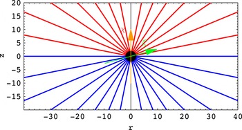
Figure 12. Topology of the infinitely thin current sheet located in the equatorial plane. In the north hemisphere, field lines are going out from the surface, red solid lines, whereas in the south hemisphere, they go into the star, blue solid lines. The observer line of sight is shown by a green arrow.
8.3 Asymptotic MHD solution
Near the neutron star, the split monopole approximation is certainly not verified or even justified. However, outside the light cylinder, the geometry of the pulsar wind can be assimilated to a split monopole. Indeed, to lowest order in
 $1/r$
, only the dipole field survives as the dominant component, and combined with a radial ideal MHD flow, field lines are stretched to eventually open and resemble to a split monopole.
$1/r$
, only the dipole field survives as the dominant component, and combined with a radial ideal MHD flow, field lines are stretched to eventually open and resemble to a split monopole.
Remember the configuration of the system. The strongly magnetized neutron star rotates along the
 $(Oz)$
axis and possesses a magnetic field assumed perfectly dipolar at its surface. The expulsion of the plasma beyond the light cylinder deforms the field lines to the point that they will open, giving rise to a situation approaching the split monopole at large distances. For an oblique rotator, making an angle
$(Oz)$
axis and possesses a magnetic field assumed perfectly dipolar at its surface. The expulsion of the plasma beyond the light cylinder deforms the field lines to the point that they will open, giving rise to a situation approaching the split monopole at large distances. For an oblique rotator, making an angle
 $\unicode[STIX]{x1D712}$
between the magnetic moment
$\unicode[STIX]{x1D712}$
between the magnetic moment
 $\unicode[STIX]{x1D741}$
and the rotation axis
$\unicode[STIX]{x1D741}$
and the rotation axis
 $\unicode[STIX]{x1D734}=\unicode[STIX]{x1D6FA}\boldsymbol{e}_{z}$
, we have
$\unicode[STIX]{x1D734}=\unicode[STIX]{x1D6FA}\boldsymbol{e}_{z}$
, we have
 $\unicode[STIX]{x1D6FA}\cos \unicode[STIX]{x1D712}=\unicode[STIX]{x1D734}\boldsymbol{\cdot }\unicode[STIX]{x1D741}$
, the surface discontinuity oscillates and propagates at the wind velocity
$\unicode[STIX]{x1D6FA}\cos \unicode[STIX]{x1D712}=\unicode[STIX]{x1D734}\boldsymbol{\cdot }\unicode[STIX]{x1D741}$
, the surface discontinuity oscillates and propagates at the wind velocity
 $V$
in the ideal MHD approximation. The flow is only in the radial direction. This surface discontinuity is determined by finding the geometric place where the magnetic field changes sign on the stellar crust. Recall that the magnetic moment in spherical coordinates is
$V$
in the ideal MHD approximation. The flow is only in the radial direction. This surface discontinuity is determined by finding the geometric place where the magnetic field changes sign on the stellar crust. Recall that the magnetic moment in spherical coordinates is
 $$\begin{eqnarray}\displaystyle \unicode[STIX]{x1D741}=\unicode[STIX]{x1D707}[\sin \unicode[STIX]{x1D712}(\cos (\unicode[STIX]{x1D6FA}t)\boldsymbol{e}_{x}+\sin (\unicode[STIX]{x1D6FA}t)\boldsymbol{e}_{y})+\cos \unicode[STIX]{x1D712}\boldsymbol{e}_{z}]. & & \displaystyle\end{eqnarray}$$
Let
 $\boldsymbol{n}$
be a unit vector pointing to the magnetic equator having components
$\boldsymbol{n}$
be a unit vector pointing to the magnetic equator having components
 $$\begin{eqnarray}\displaystyle \boldsymbol{n}=\sin \unicode[STIX]{x1D717}(\cos \unicode[STIX]{x1D711}\boldsymbol{e}_{x}+\sin \unicode[STIX]{x1D711}\boldsymbol{e}_{y})+\cos \unicode[STIX]{x1D717}\boldsymbol{e}_{z}. & & \displaystyle\end{eqnarray}$$
The magnetic equator is defined by
 $\unicode[STIX]{x1D741}\boldsymbol{\cdot }\boldsymbol{n}=0$
. The surface where the magnetic field changes polarity is therefore defined by
$\unicode[STIX]{x1D741}\boldsymbol{\cdot }\boldsymbol{n}=0$
. The surface where the magnetic field changes polarity is therefore defined by
 $$\begin{eqnarray}\displaystyle \unicode[STIX]{x1D6F9}_{s}(t,r,\unicode[STIX]{x1D717},\unicode[STIX]{x1D711})\equiv \cos \unicode[STIX]{x1D717}\cos \unicode[STIX]{x1D712}+\sin \unicode[STIX]{x1D717}\sin \unicode[STIX]{x1D712}\cos \left(\unicode[STIX]{x1D711}-\unicode[STIX]{x1D6FA}t\right)=0. & & \displaystyle\end{eqnarray}$$
This curve traced on the stellar surface is at the origin of the current sheet. Given that the plasma flow is radial and expands at a constant velocity
 $V$
, we replace the time dependence
$V$
, we replace the time dependence
 $t$
by a radial propagation term of the form
$t$
by a radial propagation term of the form
 $t-r/V$
to take into account this propagation effect. The current sheet will therefore be the geometric surface defined in 3-D space by
$t-r/V$
to take into account this propagation effect. The current sheet will therefore be the geometric surface defined in 3-D space by
 $$\begin{eqnarray}\displaystyle \unicode[STIX]{x1D6F9}_{s}(t,r,\unicode[STIX]{x1D717},\unicode[STIX]{x1D711})\equiv \cos \unicode[STIX]{x1D717}\cos \unicode[STIX]{x1D712}+\sin \unicode[STIX]{x1D717}\sin \unicode[STIX]{x1D712}\cos \left[\unicode[STIX]{x1D711}-\unicode[STIX]{x1D6FA}\left(t-\frac{r}{V}\right)\right]=0. & & \displaystyle\end{eqnarray}$$
The equation of the surface, solved for the radial variable
 $r$
, is
$r$
, is
 $$\begin{eqnarray}\displaystyle r_{s}(t,\unicode[STIX]{x1D717},\unicode[STIX]{x1D711})=\unicode[STIX]{x1D6FD}_{v}r_{L}\left[\pm \arccos (-\cot \unicode[STIX]{x1D717}\cot \unicode[STIX]{x1D712})+\frac{ct}{r_{L}}-\unicode[STIX]{x1D711}+2\ell \unicode[STIX]{x03C0}\right], & & \displaystyle\end{eqnarray}$$
where
 $\unicode[STIX]{x1D6FD}_{v}=V/c$
and
$\unicode[STIX]{x1D6FD}_{v}=V/c$
and
 $\ell$
is an integer. It is the solution found by Bogovalov (Reference Bogovalov1999). The 3-D geometry and a cross-section of the current sheet are shown in figure 13. The striped wind is therefore a spiral structure rotating at the velocity of the star and moving radially at a speed close to that of light. The current sheet is infinitely thin. In the equatorial plane (
$\ell$
is an integer. It is the solution found by Bogovalov (Reference Bogovalov1999). The 3-D geometry and a cross-section of the current sheet are shown in figure 13. The striped wind is therefore a spiral structure rotating at the velocity of the star and moving radially at a speed close to that of light. The current sheet is infinitely thin. In the equatorial plane (
 $\unicode[STIX]{x1D717}=\unicode[STIX]{x03C0}/2$
) the polar equation of the two-armed spiral is
$\unicode[STIX]{x1D717}=\unicode[STIX]{x03C0}/2$
) the polar equation of the two-armed spiral is
 $$\begin{eqnarray}\displaystyle r=\unicode[STIX]{x1D6FD}r_{L}\left(\unicode[STIX]{x1D6FA}t-\unicode[STIX]{x1D711}+\frac{\unicode[STIX]{x03C0}}{2}+\ell \unicode[STIX]{x03C0}\right). & & \displaystyle\end{eqnarray}$$
In reality, the striped wind possesses a certain thickness and an internal intrinsic dynamics not described by this simple MHD approach. For the more realistic models that we will consider, the wind is made of two plasma components, a strongly magnetised cold component outside the current layer and a weakly magnetized hot component inside the layer. The relativistic motion associated with the spiral structure is at the origin of the pulsed emission we now detail. Tchekhovskoy, Philippov & Spitkovsky (Reference Tchekhovskoy, Philippov and Spitkovsky2016) found useful approximate analytical expressions for the current in the general oblique case by fitting full 3-D force-free and MHD simulations.
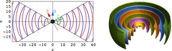
Figure 13. Topology of the infinitely thin current sheet induced by the striped wind from the split monopole. In the north hemisphere, field lines are going out from the surface, red solid lines, whereas in the south hemisphere, they go into the star, blue solid lines. The discontinuity, or magnetic polarity reversal, is depicted by this current sheet wobbling around the equatorial plane, right picture.
8.4 Origin of pulsed emission
In the striped wind scenario, the dissipation of magnetic energy happens mainly in the current sheet. Charged particles are heated to relativistic temperatures and radiate synchrotron and inverse Compton emission. If, moreover, these particles travel at a distance
 $r$
from the centre of the star such that
$r$
from the centre of the star such that
 $r\lesssim \unicode[STIX]{x1D6E4}_{v}^{2}r_{L}$
, the radiation is modulated at the rotation frequency of the neutron star. Explaining pulsation by such a mechanism was already suggested at the beginning era of pulsar theory as proposed by Michel (Reference Michel1971) and Arons (Reference Arons1979). These ideas have been reinvestigated more recently by Kirk et al. (Reference Kirk, Skjæraasen and Gallant2002). These studies showed that the striped wind is a possible site for generation of incoherent high-energy radiation, going from optical up to gamma rays. A priori, there is no reason to favour one emission site more than another, let it be outer gap, slot gap, polar cap or wind. However, compared to other models, the striped wind does not require knowledge about the inner magnetosphere and furnishes an analytical description of the magnetic field structure only based on fundamental geometrical hypotheses. This permits to circumvent the problems linked to arbitrariness of the magnetosphere.
$r\lesssim \unicode[STIX]{x1D6E4}_{v}^{2}r_{L}$
, the radiation is modulated at the rotation frequency of the neutron star. Explaining pulsation by such a mechanism was already suggested at the beginning era of pulsar theory as proposed by Michel (Reference Michel1971) and Arons (Reference Arons1979). These ideas have been reinvestigated more recently by Kirk et al. (Reference Kirk, Skjæraasen and Gallant2002). These studies showed that the striped wind is a possible site for generation of incoherent high-energy radiation, going from optical up to gamma rays. A priori, there is no reason to favour one emission site more than another, let it be outer gap, slot gap, polar cap or wind. However, compared to other models, the striped wind does not require knowledge about the inner magnetosphere and furnishes an analytical description of the magnetic field structure only based on fundamental geometrical hypotheses. This permits to circumvent the problems linked to arbitrariness of the magnetosphere.
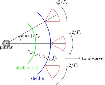
Figure 14. Principle of pulsed emission. The spherical shells propagate radially outwards with a Lorentz factor
 $\unicode[STIX]{x1D6E4}_{v}$
and emit in a cone of half-opening angle
$\unicode[STIX]{x1D6E4}_{v}$
and emit in a cone of half-opening angle
 $1/\unicode[STIX]{x1D6E4}_{v}$
when crossing the sphere of radius
$1/\unicode[STIX]{x1D6E4}_{v}$
when crossing the sphere of radius
 $R_{sph}$
, blue arc.
$R_{sph}$
, blue arc.
As stated earlier, pulsed emission is a direct consequence of the beaming induced by the relativistic flow. To better understand this phenomenon, let us assume for the sake of simplicity that the wind consists of thin, concentric spherical layers of hot radiating plasma. In the equatorial plane, successive sheets, marked by
 $n$
and
$n$
and
 $n+1$
, are separated by half a wind wavelength,
$n+1$
, are separated by half a wind wavelength,
 $\unicode[STIX]{x0394}l=\unicode[STIX]{x1D706}_{L}/2$
where
$\unicode[STIX]{x0394}l=\unicode[STIX]{x1D706}_{L}/2$
where
 $\unicode[STIX]{x1D706}_{L}=2\unicode[STIX]{x03C0}\unicode[STIX]{x1D6FD}r_{L}$
is the wind wavelength, figure 14. Moreover, assume that these sheets only radiate when crossing an imaginary sphere of radius
$\unicode[STIX]{x1D706}_{L}=2\unicode[STIX]{x03C0}\unicode[STIX]{x1D6FD}r_{L}$
is the wind wavelength, figure 14. Moreover, assume that these sheets only radiate when crossing an imaginary sphere of radius
 $R_{sph}$
, blue arc. The maximal time of arrival delay for photons emitted by the sheet, labelled
$R_{sph}$
, blue arc. The maximal time of arrival delay for photons emitted by the sheet, labelled
 $n$
, for a distant observer is
$n$
, for a distant observer is
 $\unicode[STIX]{x0394}t=\unicode[STIX]{x0394}R/c=(1-\cos \unicode[STIX]{x1D717})R_{sph}/c$
. For an ultra-relativistic flow we simplify noting that
$\unicode[STIX]{x0394}t=\unicode[STIX]{x0394}R/c=(1-\cos \unicode[STIX]{x1D717})R_{sph}/c$
. For an ultra-relativistic flow we simplify noting that
 $\unicode[STIX]{x1D717}\approx 1/\unicode[STIX]{x1D6E4}_{v}\ll 1$
. Consequently the arrival time delay is
$\unicode[STIX]{x1D717}\approx 1/\unicode[STIX]{x1D6E4}_{v}\ll 1$
. Consequently the arrival time delay is
 $$\begin{eqnarray}\displaystyle \unicode[STIX]{x0394}t\approx \frac{R_{sph}}{2\unicode[STIX]{x1D6E4}_{v}^{2}c} & & \displaystyle\end{eqnarray}$$
a well-known result from gamma-ray burst theory. To observe pulses, the delay must be inferior to the time interval elapsed between the issuance of two consecutive layers
 $n$
and
$n$
and
 $n+1$
crossing
$n+1$
crossing
 $R_{sph}$
and given by
$R_{sph}$
and given by
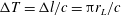 $\unicode[STIX]{x0394}T=\unicode[STIX]{x0394}l/c=\unicode[STIX]{x03C0}r_{L}/c$
. This results in a pulsed emission if (Arons Reference Arons1979)
$\unicode[STIX]{x0394}T=\unicode[STIX]{x0394}l/c=\unicode[STIX]{x03C0}r_{L}/c$
. This results in a pulsed emission if (Arons Reference Arons1979)
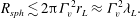 $$\begin{eqnarray}\displaystyle R_{sph}\lesssim 2\unicode[STIX]{x03C0}\unicode[STIX]{x1D6E4}_{v}^{2}r_{L}\approx \unicode[STIX]{x1D6E4}_{v}^{2}\unicode[STIX]{x1D706}_{L}. & & \displaystyle\end{eqnarray}$$
Actually this estimate is based on perfectly concentric spherical shells. In a more realistic model, care should be taken with the truly spiral structure of the wind. Thus to refine our argument, let us look at figure 15. As before the current sheet emits photons when the spiral structure crosses the sphere of radius
 $R_{sph}$
depicted as a solid black arc. The whole structure rotates rigidly in the direction indicated by the red arrow. The two magenta lines correspond to the region of the wind seen by the distant observer. One spiral arm crosses this sphere in the following order: beginning in red then middle in green and finally ending in blue as marked in figure 15. The related position in polar coordinates in the plane of the figure are noted
$R_{sph}$
depicted as a solid black arc. The whole structure rotates rigidly in the direction indicated by the red arrow. The two magenta lines correspond to the region of the wind seen by the distant observer. One spiral arm crosses this sphere in the following order: beginning in red then middle in green and finally ending in blue as marked in figure 15. The related position in polar coordinates in the plane of the figure are noted
 $(R_{sph},-\unicode[STIX]{x1D711}_{rim})$
,
$(R_{sph},-\unicode[STIX]{x1D711}_{rim})$
,
 $(R_{sph},0)$
and
$(R_{sph},0)$
and
 $(R_{sph},\unicode[STIX]{x1D711}_{rim})$
and are measured at times respectively
$(R_{sph},\unicode[STIX]{x1D711}_{rim})$
and are measured at times respectively
 $t_{-},t_{0}$
and
$t_{-},t_{0}$
and
 $t_{+}$
meanwhile emitting photons
$t_{+}$
meanwhile emitting photons
 $\unicode[STIX]{x1D6FE}_{-},\unicode[STIX]{x1D6FE}_{0}$
and
$\unicode[STIX]{x1D6FE}_{-},\unicode[STIX]{x1D6FE}_{0}$
and
 $\unicode[STIX]{x1D6FE}_{+}$
. From the spiral structure equation (8.11) these times are related by
$\unicode[STIX]{x1D6FE}_{+}$
. From the spiral structure equation (8.11) these times are related by
 $$\begin{eqnarray}\displaystyle \unicode[STIX]{x1D6FA}t_{-}+\unicode[STIX]{x1D711}_{rim}=\unicode[STIX]{x1D6FA}t_{0}=\unicode[STIX]{x1D6FA}t_{+}-\unicode[STIX]{x1D711}_{rim}, & & \displaystyle\end{eqnarray}$$
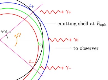
Figure 15. Real shape of the current sheet not approximated by concentric spherical shells but using the true expression in the equatorial plane. Rotation is counter-clockwise. It shows the three important phases of a pulse: begin in red, middle in green and end in blue. Photons are emitted during the whole interval
 $t\in [t_{-},t_{+}]$
, not to be confused with the reception times
$t\in [t_{-},t_{+}]$
, not to be confused with the reception times
 $t^{rec}\in [t_{-}^{rec},t_{+}^{rec}]$
, see text.
$t^{rec}\in [t_{-}^{rec},t_{+}^{rec}]$
, see text.
which leads to the ordering
 $t_{-}<t_{0}<t_{+}$
. For our purpose, in the case of a relativistic radial flow we set
$t_{-}<t_{0}<t_{+}$
. For our purpose, in the case of a relativistic radial flow we set
 $\unicode[STIX]{x1D711}_{rim}\approx 1/\unicode[STIX]{x1D6E4}_{v}$
. Taking into account time of flight of photons from the emission site to the observer we find the reception times as
$\unicode[STIX]{x1D711}_{rim}\approx 1/\unicode[STIX]{x1D6E4}_{v}$
. Taking into account time of flight of photons from the emission site to the observer we find the reception times as
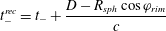 $$\begin{eqnarray}\displaystyle & \displaystyle t_{-}^{rec}=t_{-}+\frac{D-R_{sph}\cos \unicode[STIX]{x1D711}_{rim}}{c} & \displaystyle\end{eqnarray}$$
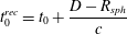 $$\begin{eqnarray}\displaystyle & \displaystyle t_{0}^{rec}=t_{0}+\frac{D-R_{sph}}{c} & \displaystyle\end{eqnarray}$$
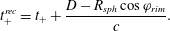 $$\begin{eqnarray}\displaystyle & \displaystyle t_{+}^{rec}=t_{+}+\frac{D-R_{sph}\cos \unicode[STIX]{x1D711}_{rim}}{c}. & \displaystyle\end{eqnarray}$$
 $t_{-}^{rec}<t_{0}^{rec}<t_{+}^{rec}$
, which must be checked a posteriori, the time observed for a pulse is of the order
$t_{-}^{rec}<t_{0}^{rec}<t_{+}^{rec}$
, which must be checked a posteriori, the time observed for a pulse is of the order 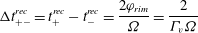 $$\begin{eqnarray}\displaystyle \unicode[STIX]{x0394}t_{+-}^{rec}=t_{+}^{rec}-t_{-}^{rec}=\frac{2\unicode[STIX]{x1D711}_{rim}}{\unicode[STIX]{x1D6FA}}=\frac{2}{\unicode[STIX]{x1D6E4}_{v}\unicode[STIX]{x1D6FA}} & & \displaystyle\end{eqnarray}$$
from which we deduce the duty cycle for one pulse as
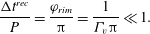 $$\begin{eqnarray}\displaystyle \frac{\unicode[STIX]{x0394}t^{rec}}{P}=\frac{\unicode[STIX]{x1D711}_{rim}}{\unicode[STIX]{x03C0}}=\frac{1}{\unicode[STIX]{x1D6E4}_{v}\unicode[STIX]{x03C0}}\ll 1. & & \displaystyle\end{eqnarray}$$
From this inequality (which holds only for
 $\unicode[STIX]{x1D6E4}_{v}\gg 1$
) we conclude that pulsation should happen at any place in the striped wind. There should be no restriction such as (8.13) where a concentric geometry was assumed. This conclusion is however incorrect. The photon
$\unicode[STIX]{x1D6E4}_{v}\gg 1$
) we conclude that pulsation should happen at any place in the striped wind. There should be no restriction such as (8.13) where a concentric geometry was assumed. This conclusion is however incorrect. The photon
 $\unicode[STIX]{x1D6FE}_{0}$
does not always succeed the photon
$\unicode[STIX]{x1D6FE}_{0}$
does not always succeed the photon
 $\unicode[STIX]{x1D6FE}_{-}$
because
$\unicode[STIX]{x1D6FE}_{-}$
because
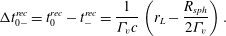 $$\begin{eqnarray}\displaystyle \unicode[STIX]{x0394}t_{0-}^{rec}=t_{0}^{rec}-t_{-}^{rec}=\frac{1}{\unicode[STIX]{x1D6E4}_{v}c}\left(r_{L}-\frac{R_{sph}}{2\unicode[STIX]{x1D6E4}_{v}}\right). & & \displaystyle\end{eqnarray}$$
It will be the case only if
 $t_{-}^{rec}<t_{0}^{rec}$
which implies
$t_{-}^{rec}<t_{0}^{rec}$
which implies
 $R_{sph}<2\unicode[STIX]{x1D6E4}_{v}r_{L}$
. In that case, the order is preserved, otherwise the photon
$R_{sph}<2\unicode[STIX]{x1D6E4}_{v}r_{L}$
. In that case, the order is preserved, otherwise the photon
 $\unicode[STIX]{x1D6FE}_{0}$
will be received before
$\unicode[STIX]{x1D6FE}_{0}$
will be received before
 $\unicode[STIX]{x1D6FE}_{-}$
even if it has been produced after the latter. The explanation lies in the additional time required by
$\unicode[STIX]{x1D6FE}_{-}$
even if it has been produced after the latter. The explanation lies in the additional time required by
 $\unicode[STIX]{x1D6FE}_{-}$
to reach the observer. According to geometrical considerations, the second condition
$\unicode[STIX]{x1D6FE}_{-}$
to reach the observer. According to geometrical considerations, the second condition
 $t_{0}^{rec}<t_{+}^{rec}$
is always satisfied independently of the distance
$t_{0}^{rec}<t_{+}^{rec}$
is always satisfied independently of the distance
 $R_{sph}$
. To observe pulsation, we require also
$R_{sph}$
. To observe pulsation, we require also
 $|\unicode[STIX]{x0394}t_{0-}^{rec}|<P$
and this gives for
$|\unicode[STIX]{x0394}t_{0-}^{rec}|<P$
and this gives for
 $\unicode[STIX]{x1D6E4}_{v}\gg 1$
a condition similar to (8.13) in the form
$\unicode[STIX]{x1D6E4}_{v}\gg 1$
a condition similar to (8.13) in the form
 $R_{sph}\lesssim 4\unicode[STIX]{x03C0}\unicode[STIX]{x1D6E4}_{v}^{2}r_{L}$
.
$R_{sph}\lesssim 4\unicode[STIX]{x03C0}\unicode[STIX]{x1D6E4}_{v}^{2}r_{L}$
.
In general, the striped wind model predicts two pulses per period, as observed in most light curves of gamma-ray pulsars, see for instance the first and second gamma-ray pulsar catalogues described in depth in Abdo et al. (Reference Abdo, Ackermann, Ajello, Anderson, Atwood, Axelsson, Baldini, Ballet, Barbiellini and Baring2009a
, Reference Abdo, Ajello, Allafort, Baldini, Ballet, Barbiellini, Baring, Bastieri, Belfiore and Bellazzini2013). The separation between these pulses is only function of the obliquity
 $\unicode[STIX]{x1D712}$
and the inclination of the line referred to as
$\unicode[STIX]{x1D712}$
and the inclination of the line referred to as
 $\unicode[STIX]{x1D701}$
. Indeed from geometric considerations about the current sheet, we derive a simple analytical relation between inclination of the line of sight
$\unicode[STIX]{x1D701}$
. Indeed from geometric considerations about the current sheet, we derive a simple analytical relation between inclination of the line of sight
 $\unicode[STIX]{x1D701}$
, obliquity of the pulsar
$\unicode[STIX]{x1D701}$
, obliquity of the pulsar
 $\unicode[STIX]{x1D712}$
and the separation between the two pulses
$\unicode[STIX]{x1D712}$
and the separation between the two pulses
 $\unicode[STIX]{x1D6E5}$
given by (Kirk Reference Kirk2005; Pétri Reference Pétri2011)
$\unicode[STIX]{x1D6E5}$
given by (Kirk Reference Kirk2005; Pétri Reference Pétri2011)
 $$\begin{eqnarray}\displaystyle |\cot \unicode[STIX]{x1D701}\cot \unicode[STIX]{x1D712}|=\cos (\unicode[STIX]{x1D6E5}\unicode[STIX]{x03C0}). & & \displaystyle\end{eqnarray}$$
For pulsars observed by Fermi/LAT, the value of
 $\unicode[STIX]{x1D6E5}$
is easily accessible. We deduce a simple relation between the two widths defining the fundamental geometry of the pulsar. Moreover with a model for radio emission, we can estimate the delay between arrival time of radio and gamma-ray photons. This has been analysed in detail in Pétri (Reference Pétri2011).
$\unicode[STIX]{x1D6E5}$
is easily accessible. We deduce a simple relation between the two widths defining the fundamental geometry of the pulsar. Moreover with a model for radio emission, we can estimate the delay between arrival time of radio and gamma-ray photons. This has been analysed in detail in Pétri (Reference Pétri2011).
Moreover for an infinitely thin sheet, the width of the pulses is inversely proportional to the Lorentz factor
 $\unicode[STIX]{x1D6E4}_{v}$
of the flow. Related to one period
$\unicode[STIX]{x1D6E4}_{v}$
of the flow. Related to one period
 $2\unicode[STIX]{x03C0}$
, this width is approximatively
$2\unicode[STIX]{x03C0}$
, this width is approximatively
 $\unicode[STIX]{x1D6E5}\approx 1/\unicode[STIX]{x03C0}\unicode[STIX]{x1D6E4}_{v}$
from (8.17). We check this with some examples of pulsed emission. More generally, when the wind is not purely in radial expansion, the criterion for existence of pulsation changes. Consider again two spherical layers separated by half a wavelength. Suppose that the plasma expansion velocity makes an angle
$\unicode[STIX]{x1D6E5}\approx 1/\unicode[STIX]{x03C0}\unicode[STIX]{x1D6E4}_{v}$
from (8.17). We check this with some examples of pulsed emission. More generally, when the wind is not purely in radial expansion, the criterion for existence of pulsation changes. Consider again two spherical layers separated by half a wavelength. Suppose that the plasma expansion velocity makes an angle
 $\unicode[STIX]{x1D6FC}$
with respect to the radial direction. The path difference between the pulse emitted in the middle and that emitted at the edge of the sheet is
$\unicode[STIX]{x1D6FC}$
with respect to the radial direction. The path difference between the pulse emitted in the middle and that emitted at the edge of the sheet is
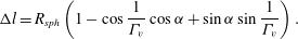 $$\begin{eqnarray}\displaystyle \unicode[STIX]{x0394}l=R_{sph}\left(1-\cos \frac{1}{\unicode[STIX]{x1D6E4}_{v}}\cos \unicode[STIX]{x1D6FC}+\sin \unicode[STIX]{x1D6FC}\sin \frac{1}{\unicode[STIX]{x1D6E4}_{v}}\right). & & \displaystyle\end{eqnarray}$$
For high Lorentz factors it simplifies into
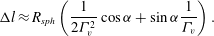 $$\begin{eqnarray}\displaystyle \unicode[STIX]{x0394}l\approx R_{sph}\left(\frac{1}{2\unicode[STIX]{x1D6E4}_{v}^{2}}\cos \unicode[STIX]{x1D6FC}+\sin \unicode[STIX]{x1D6FC}\frac{1}{\unicode[STIX]{x1D6E4}_{v}}\right). & & \displaystyle\end{eqnarray}$$
Emission will be pulsed if the difference of arrival time between the two pulses
 $\unicode[STIX]{x0394}l/c$
is less than half a period of the pulsar thus
$\unicode[STIX]{x0394}l/c$
is less than half a period of the pulsar thus
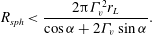 $$\begin{eqnarray}\displaystyle R_{sph}<\frac{2\unicode[STIX]{x03C0}\unicode[STIX]{x1D6E4}_{v}^{2}r_{L}}{\cos \unicode[STIX]{x1D6FC}+2\unicode[STIX]{x1D6E4}_{v}\sin \unicode[STIX]{x1D6FC}}. & & \displaystyle\end{eqnarray}$$
Two limiting cases are worthwhile
-
(i) For a strictly radial velocity with
$\unicode[STIX]{x1D6FC}=0$
we find again
$R_{sph}<2\unicode[STIX]{x03C0}\unicode[STIX]{x1D6E4}_{v}^{2}r_{L}$
. -
(ii) For a strictly azimuthal velocity with
$\unicode[STIX]{x1D6FC}=\unicode[STIX]{x03C0}/2$
we have
$R_{sph}<\unicode[STIX]{x03C0}\unicode[STIX]{x1D6E4}_{v}r_{L}$
.


Criterion (ii) is much more constraining than (i) because it is proportional to the first power of
 $\unicode[STIX]{x1D6E4}_{v}$
only and not to its second power
$\unicode[STIX]{x1D6E4}_{v}$
only and not to its second power
 $\unicode[STIX]{x1D6E4}_{v}^{2}$
. The angles
$\unicode[STIX]{x1D6E4}_{v}^{2}$
. The angles
 $\unicode[STIX]{x1D6FC}$
and
$\unicode[STIX]{x1D6FC}$
and
 $1/\unicode[STIX]{x1D6E4}_{v}$
have to be compared to check which pulse arrives first, the middle one or the edge one: the middle pulse wins if
$1/\unicode[STIX]{x1D6E4}_{v}$
have to be compared to check which pulse arrives first, the middle one or the edge one: the middle pulse wins if
 $\unicode[STIX]{x1D6FC}<1/\unicode[STIX]{x1D6E4}_{v}$
.
$\unicode[STIX]{x1D6FC}<1/\unicode[STIX]{x1D6E4}_{v}$
.
Where do we expect to produce emission? In a realistic model the current sheet possesses a finite thickness and therefore a balance between thermal and magnetic pressure in the stripes should happen. To simplify, in the two distinct regions we have
-
(i) In the current sheet: zero magnetic field
$B=0$
, constant pressure
$p$
and high particle density number
$n$
thus a hot unmagnetized plasma. -
(ii) Between the current sheet: constant magnetic field, zero pressure, low particle density number thus a cold magnetized plasma.


This entropy wave must be in MHD equilibrium in the wind rest frame such that
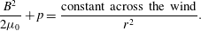 $$\begin{eqnarray}\displaystyle \frac{B^{2}}{2\unicode[STIX]{x1D707}_{0}}+p=\frac{\text{constant across the wind}}{r^{2}}. & & \displaystyle\end{eqnarray}$$
The constant has to be determined on other physical grounds.
8.5 Emission from an infinitely thin sheet
In the precedent paragraph, we explained the origin of pulses, provided that the emitting layer lies sufficiently close to the light cylinder. We now study more quantitatively this pulsed emission. The mechanisms giving rise to high-energy emission are diverse. We distinguish mainly between
-
(i) Synchrotron emission of ultra-relativistic hot electron–positron pairs in the strong magnetic field of the wind.
-
(ii) Inverse Compton emission of internal or external photons, for instance those coming from a companion, the surrounding nebula, thermal photons of the surface or synchrotron photons themselves.
The intensity of emission for the synchrotron and inverse Compton radiation is proportional to the following space–time integral
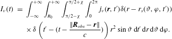 $$\begin{eqnarray}\displaystyle I_{\unicode[STIX]{x1D708}}(t) & = & \displaystyle \int _{-\infty }^{+\infty }\int _{R_{0}}^{+\infty }\int _{\unicode[STIX]{x03C0}/2-\unicode[STIX]{x1D712}}^{\unicode[STIX]{x03C0}/2+\unicode[STIX]{x1D712}}\int _{0}^{2\unicode[STIX]{x03C0}}j_{\unicode[STIX]{x1D708}}(\boldsymbol{r},t^{\prime })\unicode[STIX]{x1D6FF}(r-r_{s}(\unicode[STIX]{x1D717},\unicode[STIX]{x1D711},t^{\prime }))\nonumber\\ \displaystyle & & \displaystyle \times \,\unicode[STIX]{x1D6FF}\left(t^{\prime }-(t-\frac{\Vert \boldsymbol{R}_{obs}-\boldsymbol{r}\Vert }{c})\right)r^{2}\sin \unicode[STIX]{x1D717}\,\text{d}t^{\prime }\,\text{d}r\,\text{d}\unicode[STIX]{x1D717}\,\text{d}\unicode[STIX]{x1D711}.\end{eqnarray}$$
Integration must be performed on the current sheet making sure to include the retardation effects due to propagation at finite speed of the photons. The observer is located at the point
 $\boldsymbol{R}_{obs}$
where the unit vector is
$\boldsymbol{R}_{obs}$
where the unit vector is
 $\boldsymbol{n}_{obs}=\boldsymbol{R}_{obs}/R_{obs}$
. Emission starts at an arbitrary radius
$\boldsymbol{n}_{obs}=\boldsymbol{R}_{obs}/R_{obs}$
. Emission starts at an arbitrary radius
 $R_{0}\lesssim \unicode[STIX]{x1D6E4}_{v}^{2}r_{L}$
and
$R_{0}\lesssim \unicode[STIX]{x1D6E4}_{v}^{2}r_{L}$
and
 $t^{\prime }=t-\boldsymbol{r}\boldsymbol{\cdot }\boldsymbol{n}_{obs}/c$
corresponds to retarded time associated with emission at point
$t^{\prime }=t-\boldsymbol{r}\boldsymbol{\cdot }\boldsymbol{n}_{obs}/c$
corresponds to retarded time associated with emission at point
 $\boldsymbol{r}$
in the sheet. The Dirac distributions insure emission only when on the current sheet, thus the
$\boldsymbol{r}$
in the sheet. The Dirac distributions insure emission only when on the current sheet, thus the
 $\unicode[STIX]{x1D6FF}(r-r_{s}(\unicode[STIX]{x1D717},\unicode[STIX]{x1D711},t^{\prime }))$
term, and when the observation time is related to the retarded time of emission
$\unicode[STIX]{x1D6FF}(r-r_{s}(\unicode[STIX]{x1D717},\unicode[STIX]{x1D711},t^{\prime }))$
term, and when the observation time is related to the retarded time of emission
 $t^{\prime }$
of a photon emanating from the point
$t^{\prime }$
of a photon emanating from the point
 $\boldsymbol{r}$
on the sheet, thus the
$\boldsymbol{r}$
on the sheet, thus the
 $\unicode[STIX]{x1D6FF}(t^{\prime }-(t-\Vert \boldsymbol{R}_{obs}-\boldsymbol{r}\Vert /c))$
term.
$\unicode[STIX]{x1D6FF}(t^{\prime }-(t-\Vert \boldsymbol{R}_{obs}-\boldsymbol{r}\Vert /c))$
term.
Synchrotron and inverse Compton emissivities, far from the low- and high-frequency cutoff, are given respectively by
 $$\begin{eqnarray}\displaystyle & \displaystyle j_{\unicode[STIX]{x1D708}}^{sync}(\boldsymbol{r},t)=K_{e}(\boldsymbol{r},t)\unicode[STIX]{x1D708}^{-(p-1)/2}{\mathcal{D}}^{(p+3)/2}B^{(p+1)/2} & \displaystyle\end{eqnarray}$$
 $$\begin{eqnarray}\displaystyle & \displaystyle j_{\unicode[STIX]{x1D708}}^{IC}(\boldsymbol{r},t)=K_{e}(\boldsymbol{r},t)\unicode[STIX]{x1D708}^{-(p-1)/2}{\mathcal{D}}^{p+2}n_{\unicode[STIX]{x1D6FE}}(\unicode[STIX]{x1D700}). & \displaystyle\end{eqnarray}$$
 $$\begin{eqnarray}\displaystyle {\mathcal{D}}=\frac{1}{\unicode[STIX]{x1D6E4}_{v}(1-\boldsymbol{\unicode[STIX]{x1D6FD}}_{v}\boldsymbol{\cdot }\boldsymbol{n}_{obs})}. & & \displaystyle\end{eqnarray}$$
The power-law dependence on
 ${\mathcal{D}}$
is different for
${\mathcal{D}}$
is different for
 $j_{\unicode[STIX]{x1D708}}^{sync}$
and
$j_{\unicode[STIX]{x1D708}}^{sync}$
and
 $j_{\unicode[STIX]{x1D708}}^{IC}$
, thus affects the pulse shape depending on the distribution of particles but also following the emission process considered. The light curves exhibit peaks that are more or less pronounced. For pedagogical purposes, we show a sample of light curves for a prescribed volume emissivity. The impact of different Lorentz factors and spectral indices are shown in figure 16 for synchrotron emission and in figure 17 for inverse Compton emission. Synchrotron profiles differ from inverse Compton profiles but the general trend is the same: a decrease in the full width half maximum when the power-law index increase and/or when the Lorentz factor is augmented.
$j_{\unicode[STIX]{x1D708}}^{IC}$
, thus affects the pulse shape depending on the distribution of particles but also following the emission process considered. The light curves exhibit peaks that are more or less pronounced. For pedagogical purposes, we show a sample of light curves for a prescribed volume emissivity. The impact of different Lorentz factors and spectral indices are shown in figure 16 for synchrotron emission and in figure 17 for inverse Compton emission. Synchrotron profiles differ from inverse Compton profiles but the general trend is the same: a decrease in the full width half maximum when the power-law index increase and/or when the Lorentz factor is augmented.
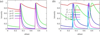
Figure 16. Sample of synchrotron emission light curves for different power-law indices
 $p=\{1,2,3,4\}$
with
$p=\{1,2,3,4\}$
with
 $\unicode[STIX]{x1D6E4}_{v}=10$
on (a) and for different Lorentz factors
$\unicode[STIX]{x1D6E4}_{v}=10$
on (a) and for different Lorentz factors
 $\unicode[STIX]{x1D6E4}_{v}=\{2,5,10,20,50\}$
with
$\unicode[STIX]{x1D6E4}_{v}=\{2,5,10,20,50\}$
with
 $p=2$
on (b). Intensities are normalized to
$p=2$
on (b). Intensities are normalized to
 $I_{max}=1$
.
$I_{max}=1$
.
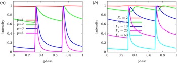
Figure 17. Sample of inverse Compton emission light curves for different power-law indices
 $p=\{1,2,3,4\}$
with
$p=\{1,2,3,4\}$
with
 $\unicode[STIX]{x1D6E4}_{v}=10$
on (a) and for different Lorentz factors
$\unicode[STIX]{x1D6E4}_{v}=10$
on (a) and for different Lorentz factors
 $\unicode[STIX]{x1D6E4}_{v}=\{2,5,10,20,50\}$
with
$\unicode[STIX]{x1D6E4}_{v}=\{2,5,10,20,50\}$
with
 $p=2$
on (b). Intensities are normalized to
$p=2$
on (b). Intensities are normalized to
 $I_{max}=1$
.
$I_{max}=1$
.
Knowing the shape of pulses for a given frequency, now we are interested in the spectral power density from this radiation. We have seen that pulsed emission comes from relativistic Doppler beaming. The exact function of this dependence in the Doppler factor is determined by the same power-law spectral density. It is therefore essential to know this spectral power density for estimating the shape of the pulses at a given frequency. We study the synchrotron and inverse Compton emission. Emissivity is chosen so as to include the power-law dependence of the frequency of observation considered. The shape of the pulses depend not only on the Lorentz factor of the wind and the emission process itself, inverse compton (IC) or synchrotron, but also on the observation frequency before the low cutoff, between the two cutoff frequencies and after the high-frequency cutoff. Light curves are shown in the case of inverse Compton emission of the gamma-ray binary PSR B1259-63 in Pétri & Dubus (Reference Pétri and Dubus2011). In the striped wind model for high-energy emission, we observe a natural narrowing of the pulse width at highest energies due to the increased sensitivity on relativistic beaming.
8.6 Emission of a more realistic model
In reality, the current sheet in the striped wind is not infinitely thin but possesses a finite thickness defined by its internal dynamics and therefore a spatial extension induced by pressure in the gas heated to relativistic temperatures. To account for this finite thickness of the current sheet, it is necessary to integrate emissivity in the whole 3-D volume of the wind and not only on the 2-D current sheet. To extract meaningful light-curves we need to set the parameters of a realistic wind model. These can be divided into three groups
-
(i) Geometrical properties:
-
(a) The obliquity
$\unicode[STIX]{x1D712}$
of the pulsar. -
(b) The inclination
$\unicode[STIX]{x1D701}$
of the line of sight with respect to rotation axis.
-
-
(ii) Magnetic field configuration:
-
(a) No radial component
$B_{r}=0$
but toroidal components given by
$B_{\unicode[STIX]{x1D703}},B_{\unicode[STIX]{x1D711}}\propto 1/r$
. -
(b) The current sheet represented as a discontinuous
$B_{\unicode[STIX]{x1D711}}$
, replaced by a transition layer of thickness
$(\unicode[STIX]{x1D6E5}_{\unicode[STIX]{x1D711}})$
inducing a smooth
$B_{\unicode[STIX]{x1D711}}$
polarity reversal. -
(c) Accompanied by a significant
$B_{\unicode[STIX]{x1D703}}$
component in the current sheet.
-
-
(iii) Dynamical properties (emitting particles):
-
(a) The Lorentz factor
$\unicode[STIX]{x1D6E4}_{v}$
of the wind. -
(b) The power-law index
$p$
of the particle distribution. -
(c) The electron/positron number density
$K(\boldsymbol{r},t)$
such that the distribution function, isotropic in momentum space
$\boldsymbol{{\mathcal{P}}}$
, is (8.27)Pressure balance implies that a strong magnetic field is associated with low density plasma and conversely.
$$\begin{eqnarray}\displaystyle N(E,\boldsymbol{{\mathcal{P}}},\boldsymbol{r},t)=K(\boldsymbol{r},t)E^{-p}. & & \displaystyle\end{eqnarray}$$
-


We keep the structure of the split monopole but consider only the toroidal component
 $B_{\unicode[STIX]{x1D711}}$
, the two other components being negligible. So the wind velocity is perpendicular to the magnetic field which simplifies Lorentz transformation of the electromagnetic field between wind frame and observer frame. Pulsed emission arises in the striped wind via inverse Compton radiation from synchrotron photons from the nebula or cosmic microwave background. Particle distribution is monoenergetic. This method is applied to Geminga, see the phase resolved spectra in Pétri (Reference Pétri2009a
). Moreover Petri (Reference Petri2012) showed that the gamma-ray luminosity of Fermi/LAT pulsars can be interpreted as synchrotron emission from the striped wind current sheet as already mentioned by Lyubarskii (Reference Lyubarskii1996). In a stationary state, the radiative losses are compensated by magnetically reheated particles through magnetic reconnection. The Lorentz factor of the wind is then estimated as well as the reconnection rate in the relativistic plasma. Arka & Dubus (Reference Arka and Dubus2013) investigated the properties of synchrotron radiation in the current sheet assuming a thermal population of particles and found spectra that peak around the GeV with gamma-ray efficiency in agreement with Fermi/LAT observations. However, due to magnetic reconnection in the stripes, Mochol & Pétri (Reference Mochol and Pétri2015) identified two regimes of particle acceleration, the first limited by radiation reaction and the second by the size of the accelerating region that strongly impacts on the pulsed inverse Compton spectra in the sub-TeV band. Reconnection in the current sheet has also been investigated by Uzdensky & Spitkovsky (Reference Uzdensky and Spitkovsky2014).
$B_{\unicode[STIX]{x1D711}}$
, the two other components being negligible. So the wind velocity is perpendicular to the magnetic field which simplifies Lorentz transformation of the electromagnetic field between wind frame and observer frame. Pulsed emission arises in the striped wind via inverse Compton radiation from synchrotron photons from the nebula or cosmic microwave background. Particle distribution is monoenergetic. This method is applied to Geminga, see the phase resolved spectra in Pétri (Reference Pétri2009a
). Moreover Petri (Reference Petri2012) showed that the gamma-ray luminosity of Fermi/LAT pulsars can be interpreted as synchrotron emission from the striped wind current sheet as already mentioned by Lyubarskii (Reference Lyubarskii1996). In a stationary state, the radiative losses are compensated by magnetically reheated particles through magnetic reconnection. The Lorentz factor of the wind is then estimated as well as the reconnection rate in the relativistic plasma. Arka & Dubus (Reference Arka and Dubus2013) investigated the properties of synchrotron radiation in the current sheet assuming a thermal population of particles and found spectra that peak around the GeV with gamma-ray efficiency in agreement with Fermi/LAT observations. However, due to magnetic reconnection in the stripes, Mochol & Pétri (Reference Mochol and Pétri2015) identified two regimes of particle acceleration, the first limited by radiation reaction and the second by the size of the accelerating region that strongly impacts on the pulsed inverse Compton spectra in the sub-TeV band. Reconnection in the current sheet has also been investigated by Uzdensky & Spitkovsky (Reference Uzdensky and Spitkovsky2014).
For binary systems with two neutron stars of which at least one is a pulsar, geodetic precession causes a secular variation in the inclination of the line of sight. We deduce a variation in the light curve not only in radio but also at higher energies, including X-rays and gamma rays. We therefore used the striped wind model to compute these phase-resolved light curves. Some systems will possibly permit a detection of this precession in the decades ahead, as was shown in Pétri (Reference Pétri2015b ).
But the striped wind could also be responsible for a non-pulsed emission causing giant gamma-ray flares around 400 MeV lasting for hours to days as noted by Striani et al. (Reference Striani, Tavani, Piano, Donnarumma, Pucella, Vittorini, Bulgarelli, Trois, Pittori and Verrecchia2011), Buehler et al. (Reference Buehler, Scargle, Blandford, Baldini, Baring, Belfiore, Charles, Chiang, D’Ammando and Dermer2012) and Striani et al. (Reference Striani, Tavani, Vittorini, Donnarumma, Giuliani, Pucella, Argan, Bulgarelli, Colafrancesco and Cardillo2013). Baty, Petri & Zenitani (Reference Baty, Petri and Zenitani2013) have interpreted this phenomenon as a signature of relativistic magnetic reconnection operating explosively in the striped wind due to instability caused by the presence of several neighbouring current sheets. Already two alternations of the field are sufficient to get violent reconnection. This is known as the double tearing mode. The Baty et al. (Reference Baty, Petri and Zenitani2013) work was followed by some numerical improvements (Pétri et al. Reference Pétri, Takamoto, Baty and Zenitani2015) and extraction of the synchrotron radiation signature in a post-processing procedure (Takamoto, Pétri & Baty Reference Takamoto, Pétri and Baty2015).
Force-free simulations have shown that the wind outside the light cylinder resembles the split monopole solution with a dominant toroidal magnetic field component. The split monopole is a simple and good analytical solution at large distances but inadequate to represent the closed magnetosphere. It is therefore illuminating to compare the phase shift in the two-armed spirals found in the striped wind, vacuum and force-free solutions for the orthogonal rotator. The results of this comparison is shown in figure 18. The shift is evident and the ordering is, vacuum first, force-free second and split monopole third. So we conclude that using the split monopole to compute simultaneously polar cap radio emission and current sheet high-energy emission leads to a time lag between both pulses which is not the same as for the more realistic force-free solution. If the dipole geometry inside the light cylinder is taken into account, we expect the delay between radio and gamma-ray emission to be less than the lags reported in Pétri (Reference Pétri2011). This can explain the 0.1 phase excess noted in this earlier work.
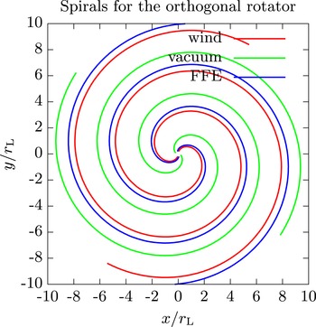
Figure 18. Comparison of the location of the spiral structure for the striped wind (red), the vacuum (green) and the force-free (blue) solution for the orthogonal rotator. In current sheet models, dissipation and radiation outside the light cylinder essentially occurs within a small thickness around this spiral region.
8.7 Kinetic aspects related to the current sheet
The physical conditions inside the current sheet are badly constraints. A detailed description would require the modelling of the overall electromagnetic circuitry in the magnetosphere and even beyond the light cylinder. Unfortunately, such studies are still not available to a sufficient level of refinement. Also, we have to restrict ourselves by a formulating hypothesis that one can judge more or less reasonable only based on the observational consequences that will be drawn. It seems that several pulsars emitting mainly in gamma rays show light curves possessing not two but three or four distinct peaks. It is already clear that Vela exhibits a third pulse. Moreover, this third pulse drifts with frequency (Abdo et al.
Reference Abdo, Ackermann, Atwood, Bagagli, Baldini, Ballet, Band, Barbiellini, Baring and Bartelt2009b
). This observation tends therefore to eliminate the striped wind model because it only predicts two pulses per rotation, one for each polarity of the current sheet, sometimes linked to the north pole sometimes to the south pole. The nature of the stripes combined to a drift motion of the
 $e^{\pm }$
pairs in different directions leads to an important modification of the light curve shape. We could expect up to four pulses, more or less well separated, depending on the internal dynamics in the current sheet.
$e^{\pm }$
pairs in different directions leads to an important modification of the light curve shape. We could expect up to four pulses, more or less well separated, depending on the internal dynamics in the current sheet.
From a more fundamental point of view, Pétri & Kirk (Reference Pétri and Kirk2007a ,Reference Pétri and Kirk b ) have studied in detail the kinetic aspects related to the tearing instability for a relativistic current sheet and for the Weibel instability via a linear analysis of the Vlasov–Maxwell equations. In the longer term simulations of reconnection will benefit from a relativistic approach including kinetic works previously cited. It could also be supplemented with radiation effects that are dominant in the stripes.
8.8 Polarization of the synchrotron pulsed emission
To probe the structure of any magnetic field, measurement of synchrotron emission polarization is often invoked. Synchrotron emission indeed shows a high degree of linear polarization when the magnetic field in which bathes the leptons is ordered. The striped wind magnetic field possesses such ordered topology. We therefore expect to observe a specific pulsed polarisation signature in the emission of the wind. Fortunately such observations exist for at least one pulsar. Indeed Słowikowska et al. (Reference Słowikowska, Kanbach, Kramer and Stefanescu2009) have reported with high precision the optical phase-resolved polarization properties of the Crab pulsar. A study of the polarization of the synchrotron emission is strongly discriminating for later comparison between models and observations.
The polarisation of total emission of the wind is performed by summation on the distribution function of emitting particles, here the electrons, that are integrated in 3-D space and for all time. Electrons are assumed to possess a stationary distribution independent of time, be isotropic in momentum and follow a power law in energy. The asymptotic structure of the field such that given by the ideal MHD cannot give information about the field interior to the current sheet. It is seen as a singularity. Actually, it has a finite thickness and an inner structure, but the distribution of particles and magnetic field are still inaccessible to simulations. We have no choice but to prescribe a priori its characteristics. Comparisons between our model and observations of pulsed emission at optical wavelengths by Słowikowska et al. (Reference Słowikowska, Kanbach, Kramer and Stefanescu2009) are shown in Pétri & Kirk (Reference Pétri and Kirk2005). Agreement between our model and these data are satisfactory. However, a
 $B_{\unicode[STIX]{x1D717}}$
component was necessary to fit properly the data. A complete catalogue of polarization properties from pulsed synchrotron emission has been compiled for all possible geometries. The results have been synthesized in Pétri (Reference Pétri2013b
) using a slightly different prescription for radiation in the cold and hot part of the wind. Comparing the expectations about phase-resolved polarisation in the optical region from several models, as presented by Dyks, Harding & Rudak (Reference Dyks, Harding and Rudak2004), and our wind model in Pétri & Kirk (Reference Pétri and Kirk2005), it is obvious that firm conclusions could be drawn from such observations. Unfortunately, we still await an instrument able to detect the linear polarisation of photons above several tenths of an eV with also a sufficient temporal resolution. Attempts to use current technology such as INTEGRAL to search for linearly polarized emission above 200 keV have been conducted by Forot et al. (Reference Forot, Laurent, Grenier, Gouiffès and Lebrun2008) who found in a survey of the Crab Nebula a strong signal polarized along the pulsar rotation axis with some improvements from Chauvin et al. (Reference Chauvin, Roques, Clark and Jourdain2013). INTEGRAL was also used by Dean et al. (Reference Dean, Clark, Stephen, McBride, Bassani, Bazzano, Bird, Hill, Shaw and Ubertini2008) to detected gamma-ray polarized emission from the Crab. Recently Chauvin et al. (Reference Chauvin, Florén, Jackson, Kamae, Kawano, Kiss, Kole, Mikhalev, Moretti and Olofsson2016) reported hard X-ray polarization measurements of the Crab pulsar with a balloon-borne polarimeter called PoGOLite (Kamae et al.
Reference Kamae, Andersson, Arimoto, Axelsson, Marini Bettolo, Björnsson, Bogaert, Carlson, Craig and Ekeberg2008).
$B_{\unicode[STIX]{x1D717}}$
component was necessary to fit properly the data. A complete catalogue of polarization properties from pulsed synchrotron emission has been compiled for all possible geometries. The results have been synthesized in Pétri (Reference Pétri2013b
) using a slightly different prescription for radiation in the cold and hot part of the wind. Comparing the expectations about phase-resolved polarisation in the optical region from several models, as presented by Dyks, Harding & Rudak (Reference Dyks, Harding and Rudak2004), and our wind model in Pétri & Kirk (Reference Pétri and Kirk2005), it is obvious that firm conclusions could be drawn from such observations. Unfortunately, we still await an instrument able to detect the linear polarisation of photons above several tenths of an eV with also a sufficient temporal resolution. Attempts to use current technology such as INTEGRAL to search for linearly polarized emission above 200 keV have been conducted by Forot et al. (Reference Forot, Laurent, Grenier, Gouiffès and Lebrun2008) who found in a survey of the Crab Nebula a strong signal polarized along the pulsar rotation axis with some improvements from Chauvin et al. (Reference Chauvin, Roques, Clark and Jourdain2013). INTEGRAL was also used by Dean et al. (Reference Dean, Clark, Stephen, McBride, Bassani, Bazzano, Bird, Hill, Shaw and Ubertini2008) to detected gamma-ray polarized emission from the Crab. Recently Chauvin et al. (Reference Chauvin, Florén, Jackson, Kamae, Kawano, Kiss, Kole, Mikhalev, Moretti and Olofsson2016) reported hard X-ray polarization measurements of the Crab pulsar with a balloon-borne polarimeter called PoGOLite (Kamae et al.
Reference Kamae, Andersson, Arimoto, Axelsson, Marini Bettolo, Björnsson, Bogaert, Carlson, Craig and Ekeberg2008).
There is still a strong debate about the precise location of pulsed high-energy emission from pulsars. However, the general consensus now is that it must come from regions close to or outside the light cylinder.
9 Summary
Neutron stars and their most frequent observational manifestations as pulsars are exquisite space laboratories to explore physics under extreme gravitational and electromagnetic fields. However, in order to correctly interpret the multi-wavelength signal detected on Earth, we need a better understanding of the interrelations between the electromagnetic field, the gravitational field, the plasma and the radiation field. We are still far from a complete and exhaustive answer to the physics taking place in pulsar magnetosphere. Our sparse ideas need more thorough and systematic investigations. The wealth of observational data at all wavelengths acquired from systems containing a neutron star (isolated pulsars, isolated neutron stars, magnetars, binary pulsars) complicates our tentative attempts to synthesize the subject in a clear manner. Most importantly, it renders our task difficult in terms of extracting useful information.
However, efforts have been made towards a more self-consistent treatment of the electromagnetic, gravitational, plasma and radiation interactions leading to more quantitative results. Numerical simulations promise to unveil some aspects of pulsar physics but the huge gaps between the microphysics and the global structure of this system requires even more clever ideas to perform realistic meaningful simulations. Improvement in numerical algorithms are certainly welcome but it is hopeless to expect to gain the final answer simply by running such codes, claimed to contain all the physics starting from first principles. Simulations must be taken with caution and we should never forget that numerical simulations are useful to encourage critical thinking rather than being a substitute to brainwork.
10 For further information
For a thorough discussion on several important aspects of pulsar dynamics to more than an introductory level, the reader is referred to some excellent books. For instance Michel (Reference Michel1991) although outmoded from an observational point of view, contains a still topical and interesting theoretical description of neutron stars magnetosphere. Beskin et al. (Reference Beskin, Gurevich and Istomin1993) discuss in details the kinetic aspects of magnetospheric plasma with pair creation and radiation mechanisms. Accretion powered pulsars offer some other insight into neutron star magnetospheric physics (Ghosh Reference Ghosh2007). The two last chapters of Mestel (Reference Mestel1999) are devoted to pulsar electrodynamics. Michel & Li (Reference Michel and Li1999) proposed a pedagogical and convincing discussion of the usefulness of non-neutral plasmas in the context of pulsars. The general theory of these non-neutral plasmas is presented in depth by Davidson (Reference Davidson1990).


