


1. Introduction
Interaction between the wall boundary layer and blunt body wake is widely encountered in engineering applications, such as pipelines near the ground, multi-airfoil configuration, and turbo-machinery (Squire Reference Squire1989; Ovchinnikov, Piomelli & Choudhari Reference Ovchinnikov, Piomelli and Choudhari2006; Durbin & Wu Reference Durbin and Wu2007). Such wake/boundary layer interactions substantially change the flow pattern and the dynamic forces acting on the bodies. There are also complex coherent vortical structures generated during the interactions. It is essential to understand the wake/boundary layer interactions for engineering design. The simplified model of flow past a circular cylinder with diameter  $D$ transversely placed above a plane wall with wall-normal gap $G$ is usually adopted to study the complicated fluid dynamics.
It is well known that there is vortex shedding for flow around an isolated circular cylinder at a supercritical Reynolds number. With the vortex shedding from the cylinder, the local pressure near the cylinder is altered which causes the fluctuating drag and lift of the cylinder. When the cylinder is placed near the plane wall, the aerodynamic forces acting on the cylinder are changed. The vortex shedding frequency is influenced by both the gap ratio  $G/D$ and the thickness of the boundary layer $\delta _D$ (Zdravkovich Reference Zdravkovich1985; Lei, Cheng & Kavanagh Reference Lei, Cheng and Kavanagh1999). Generally, $\delta _D$ is the laminar or turbulent boundary layer thickness at the cylinder position in the absence of the cylinder. The lift, drag and vortex shedding frequency can be expressed as the lift coefficient $C_{L}$, the drag coefficient $C_{D}$ and the Strouhal number $St$ in non-dimensional forms, respectively. The Reynolds number based on the cylinder diameter is denoted as $Re_D$.
Bearman & Zdravkovich (Reference Bearman and Zdravkovich1978) investigated the flow over a circular cylinder positioned at various heights above a plate in a wind tunnel. The turbulent boundary layer thickness  $\delta _D$ at the cylinder position was fixed to 0.8 $D$. They conducted hot-wire measurements at $Re_D=2.5 \times 10^{4}$ as well as mean pressure measurements at $Re_D=4.5 \times 10^{4}$. Hot-wire signals revealed that the vortex shedding can not only be suppressed but completely ceased at small gap ratios. The wake flow was found to be intermittent at $G/D=0.4$ and the vortex shedding frequency $St$ became constant at $G/D=0.3$. The distribution of mean pressure showed that the presence of the wall significantly changed the symmetry of the pressure field. Zdravkovich (Reference Zdravkovich1985) measured the drag and lift force acting on the cylinder in a range of $Re_D$ from $4.8 \times 10^{4}$ to $3.0 \times 10^{5}$. The gap ratio and the thickness of the boundary layer were varied in $0< G/D<2$ and $0.12<\delta _D /D <0.97$, respectively. It was found that the drag coefficient $C_D$ was constant when the cylinder was placed out of the boundary layer. When the cylinder was moved into the turbulent boundary layer, $C_D$ decreased with decreasing $G/\delta _D$. It was claimed that the drag coefficient was dominated by $G/\delta _D$, but the lift coefficient $C_L$ was governed by $G/D$. Buresti & Lanciotti (Reference Buresti and Lanciotti1992) experimentally measured the lift in a similar boundary layer with that of Zdravkovich (Reference Zdravkovich1985). They found that $C_L$ rapidly decreased with increasing $G/D$, whereas $C_D$ depended on $Re_D$ and was affected by $\delta _D$. Lei et al. (Reference Lei, Cheng and Kavanagh1999) also experimentally investigated the hydrodynamic forces and vortex shedding in a range of $Re_D$ from $1.3 \times 10^{4}$ to $1.45 \times 10^{4}$. The measured lift coefficient decreased more rapidly in the thicker boundary layers than in the thinner boundary layers, even negative $C_L$ was obtained for $0.4< G/D<1.2$.
Price et al. (Reference Price, Sumner, Smith, Leong and Paidoussis2002) employed particle image velocimetry (PIV) and hot-film anemometry to study the flow around a circular cylinder near to a plane wall for  $1200 \leqslant Re_D \leqslant 4960$ and $0 \leqslant G/D \leqslant 2$. The flow was classified into four distinct regimes. For $G/D \leqslant 0.125$, it was found that the gap flow was suppressed with the wall boundary layer separated from both upstream and downstream of the cylinder. Although no regular vortex shedding occurred, there was a periodicity detected in the upper shear layer of the cylinder. When $0.125 < G/D < 0.5$, the characteristics of the flow were very similar to that for $G/D \leqslant 0.125$, except that a pronounced pairing between the wall boundary layer and the shear layer shed from the lower side of the cylinder was observed. For $0.5 < G/D < 0.75$, the flow was characterized by the onset of vortex shedding from the cylinder. For the fourth region, $G/D >1.0$ considered as the largest gap ratio, there is no separation of the wall boundary layer, either upstream or downstream of the cylinder. Furthermore, the flow was the same as the flow around an isolated circular cylinder. For the vortex shedding frequency $St$, Price et al. (Reference Price, Sumner, Smith, Leong and Paidoussis2002) revealed that $St$ is almost independent of both $G/D$ and $\delta _D$ for $Re_D \geqslant 1.3\times 10^{4}$ and $0.1\leqslant \delta _D/D \leqslant 1.64$. However, they found that $St$ is much more sensitive to $G/D$ at a low Reynolds number, and a similar result has been reported by Lin et al. (Reference Lin, Lin, Hsieh and Dey2009) and He et al. (Reference He, Wang, Pan, Feng, Gao and Rinoshika2017).
Wang & Tan (Reference Wang and Tan2008) experimentally studied the near wake of a cylinder placed close to a fully developed turbulent boundary. The  $Re_D$ was $1.2 \times 10^{4}$ and $G/D$ ranged from 0.1 to 1.0. Periodic vortex shedding from the upper and lower sides of the cylinder was observed for $G/D \geqslant 0.3$. When $G/D\leqslant 0.6$, the wake flow was asymmetric about the cylinder centreline. Sarkar & Sarkar (Reference Sarkar and Sarkar2009, Reference Sarkar and Sarkar2010) performed large eddy simulations (LES) for $Re_D=1440$ and $G/D=0.25$, 0.5, 1.0, and revealed that the shear layer instability, small-scale motion and modification of wake dynamics apart from its coherent structure are strongly influenced by $G/D$. For $G<\delta _D$, the coupling of the inner shear layer with the wall boundary layer delayed the shear instability and the appearance of a spanwise structure. The interactions between the secondary vortices and the wake vortices lead to an inversion of the upper wake vortex and the lower wake vortex.
He et al. (Reference He, Wang, Pan, Feng, Gao and Rinoshika2017) investigated the dynamics of vortical structures for  $Re_D=1072$ and $G/D$ from 0 to 3.0. A boundary layer separation was induced on the flat plate downstream of the cylinder when $G/D \leqslant 2.0$. The wake of the cylinder became asymmetric as the cylinder approached the wall. Based on the phase-averaged flow and virtual dye visualization in the instantaneous PIV velocity field, the vortex dynamics were investigated for $G/D=0.5$, $1.0$ and 2.0. When $G/D=2.0$, the secondary spanwise vortices were periodically induced near the wall by the cylinder wake vortices. When $G/D=1.0$, the secondary vortex directly interacted with the lower wake vortex. For $G/D=0.5$, the approaching of the wall led to the more complex interactions among the upper wake vortex, the lower wake vortex and the secondary vortex. Furthermore, the coloured virtual dye visualizations revealed the breakdown of the vortices into filamentary debris during the interactions. A similar vortex evolution has been reported by Zhou et al. (Reference Zhou, Qiu, Li and Liu2021) recently with the proper orthogonal decomposition and the vortex identification method. While He, Pan & Wang (Reference He, Pan and Wang2013a) found that the secondary vortices can be either entrained into the rollers or pushed down towards the wall at $G/D=1.0$.
Ouro, Muhawenimana & Wilson (Reference Ouro, Muhawenimana and Wilson2019) elucidated the near-wake dynamics developed behind a cylinder with wall proximity effects from the experiments and LES. Here  $G/D$ was fixed as 0.5 and 1.0 for $Re_D=6666$, 10 000 and 13 333. While the height in the wall-normal direction was only $3D$ with free-surface effects considered, which is completely different from the conditions in previous studies. The dynamics of the vortex generation and shedding were significantly influenced by the wall, which led to an increasingly asymmetric wake distribution with increasing $Re_D$. However, the wake at $G/D=1.0$ was relatively symmetric. Because of the high Reynolds numbers, Kelvin–Helmholtz (KH) instabilities developed both in the upper and lower layers of the cylinder. The shear layers, following the KH instabilities, were broken down into small vortices that were convected downstream, eventually merging with the fully turbulent wake. Note that spanwise rollers in the near wake were formed with an undulating shape instead of being parallel to the cylinder. And the rollers exhibited a wavelength $\lambda$ of approximately ${\rm \pi} D/2$. Furthermore, the second vortices induced by the lower vortex lifted off the wall and merged with the Kármán vortex to form a single vortical structure.
Apart from the above research focusing on the aerodynamic forces acting on the cylinder and gap ratio effects on the wake pattern, there are also some studies paying more attention to the transition of the wall boundary layer influenced by the perturbations of the wake. Kyriakides et al. (Reference Kyriakides, Kastrinakis, Nychas and Goulas1999) experimentally investigated the flat-plate boundary layer transition induced by the wake of a cylinder from the point of view of the occurring coherent structures when  $Re_D=3500$ and $G/D=2.5$. Through the analysis of the signals, during the transition, a secondary spanwise vortical structure with concentrated spanwise vorticity appeared near the wall. Ovchinnikov et al. (Reference Ovchinnikov, Piomelli and Choudhari2006) carried out the interaction between a laminar boundary layer and a Kármán vortex street behind a circular cylinder using direct numerical simulation (DNS) and LES for $Re_D=385$, 1155, $3900$ and $G/D=3.5$. They observed bypass-like transition (Morkovin Reference Morkovin1969) to turbulence in two higher Reynolds number cases. The results showed that the transition process had similarities in turbulent statistics and streaky structures induced by free-stream turbulence (FST) (Kendall Reference Kendall1998; Jacobs & Durbin Reference Jacobs and Durbin2001; Matsubara & Alfredsson Reference Matsubara and Alfredsson2001). Although streaky structures appearing inside the boundary layer led to a transition to turbulence, Ovchinnikov et al. (Reference Ovchinnikov, Piomelli and Choudhari2006) claimed that it is distinctly different for these two transition scenarios in terms of the external perturbation and transition mechanism. Note that Ovchinnikov et al. (Reference Ovchinnikov, Piomelli and Choudhari2006) did not find any secondary spanwise vortical structures inside the boundary layer; however, streaky structures have not been reported by Kyriakides et al. (Reference Kyriakides, Kastrinakis, Nychas and Goulas1999).
Pan et al. (Reference Pan, Wang, Zhang and Feng2008) investigated flat-plate boundary layer transition induced by the wake of a circular cylinder for  $Re_D=2000$ and $G/D=3.15$ and 4. A different transition route from the Klebanoff mode (Klebanoff, Tidstrom & Sargent Reference Klebanoff, Tidstrom and Sargent1962; Klebanoff Reference Klebanoff1971; Kendall Reference Kendall1985) in FST induced transition was reported. The visualization study revealed that the secondary spanwise vortical structures were induced by the wake vortex street of the cylinder near the flat-plate surface, periodically. Then these secondary vortices evolved into $\varLambda$/hairpin vortices, which were the feature of the boundary layer transition. Furthermore, the primary hairpins from secondary vortices could generate new hairpins through the parent-offspring scenario (Schoppa & Hussain Reference Schoppa and Hussain2002), which led to the formation of the streamwise elongated hairpin packets in the final turbulent boundary layer. The spanwise vortices appearing in the early stage and evolving into $\varLambda /{\rm hairpin}$ vortices were confirmed by Mandal & Dey (Reference Mandal and Dey2011). He, Wang & Pan (Reference He, Wang and Pan2013b) experimentally investigated the initial growth of a disturbance induced by the wake of the cylinder in the flat-plate boundary layer when $Re_D=1118$ and $G/D=1.8$. The streamwise variation of the disturbance energy within the boundary layer showed a two stage growth, which were both associated with the evolution of secondary vortices. He et al. (Reference He, Pan, Feng, Gao and Wang2016) investigated the evolution of Lagrangian coherent structures (LCS) in a flat-plate boundary layer transition induced by the wake of a circular cylinder when $Re_D=1072$ and $G/D=2.0$ using quantitative finite-time Lyapunov exponents (FTLE). It was the first time that the mean convection velocity and average inclination angle of the LCS were extracted from the FTLE fields.
As shown above, there have been many studies focusing on the flow around a cylinder placed near the wall, however, most of the previous studies are based on experiments with hot wires and two-dimensional PIV. The details in three-dimensional vortex dynamics are yet to be explored, especially at small gap ratios with complex wake/wall boundary layer interactions. Therefore, in this study we uniquely explore the detailed three-dimensional vortex dynamics, including the vortex interactions and hairpin vortices generation, at small gap ratios by performing DNS. Furthermore, the wake-induced transition scenarios at small gap ratios have been less discussed in the above-mentioned research. We are thus motivated to depict the important receptivity process at small gap ratios. It is hoped that this study can cast some light on the research of the vortex dynamics and wake-induced boundary layer transition. The rest of the paper is arranged as follows. The physical model and numerical method are given in § 2. Section 3 reports the main results. Finally, § 4 gives the conclusion.
2. Numerical set-up
2.1. Flow configuration and numerical method
Figure 1 shows the sketch of flow past a cylinder in proximity to a plane wall. The cylinder with diameter  $D$ is placed $10D$ from the inlet and the outlet is $50D$ downstream from the cylinder. The gap from the lower surface of the cylinder to the plane wall is denoted as $G$. The domain is extended up to $L_y=10D$ and $L_z=2{\rm \pi} D$ in the wall-normal and spanwise directions, respectively. The domain is set following the literature (Ovchinnikov et al. Reference Ovchinnikov, Piomelli and Choudhari2006; Sarkar & Sarkar Reference Sarkar and Sarkar2009, Reference Sarkar and Sarkar2010; Ouro et al. Reference Ouro, Muhawenimana and Wilson2019). The governing equations are the dimensionless Navier–Stokes equations for incompressible, viscous flow that are solved in the Cartesian coordinate system, and are as follows:
 $$\begin{gather} \boldsymbol{\nabla}\boldsymbol{\cdot} \boldsymbol{u}=0, \end{gather}$$
 $$\begin{gather}\frac{\partial \boldsymbol{u}}{\partial t}+\boldsymbol{u}\boldsymbol{\cdot}\boldsymbol{\nabla}\boldsymbol{u}={-}\boldsymbol{\nabla} p+\frac{1}{Re_D}\nabla^{2}\boldsymbol{u}. \end{gather}$$
Here,  $\boldsymbol {u}\equiv (u,v,w)$ is the velocity vector, $t$ is the time, $p$ is the pressure. The Reynolds number $Re_D=U_0 D/\nu$ is defined based on the circular cylinder diameter $D$ and the inflow velocity $U_0$, where $\nu$ is the kinematic viscosity. Here $Re_D$ is fixed at 1000 in this study. The gap ratio $G/D$ ranges from 0.1 to 0.9.
The sketch of flow past a circular cylinder placed near a plane wall.

Following the literature (He et al. Reference He, Pan and Wang2013a; Zhou et al. Reference Zhou, Qiu, Li and Liu2021), the Blasius profile with boundary layer thickness  $\delta _0=0.492D$ is imposed at the inlet, which makes $\delta _D=0.7D$. No-slip boundary condition ( $u=v=w=0$) is applied on the plane wall and on the cylinder surface. The far field condition ( $\partial u/\partial y=0, v=0, \partial w/\partial y=0$) is imposed along the upper surface of the domain. The high-order outflow boundary condition is imposed at the outlet (Dong, Karniadakis & Chryssostomidis Reference Dong, Karniadakis and Chryssostomidis2014).
The numerical simulations are performed using the Fourier spectral/hp element method (Bolis Reference Bolis2013) embedded in the open source code Nektar++ (Cantwell et al. Reference Cantwell2015; Moxey et al. Reference Moxey2020). The problem is discretized spatially in the  $(x, y)$ plane and a Fourier expansion in the $z$ direction to reveal the three-dimensional features of the flow (Bolis Reference Bolis2013). In the two-dimensional domain the spatial resolution is controlled by the distribution of h-type elements with $P$-order interpolation polynomials for the p-type expansion. Under the assumption of being homogeneous in the spanwise direction, the three-dimensional flow is resolved by introducing Fourier expansion in the spanwise direction. If $N$ Fourier planes are used, the spanwise resolution is $2N$.
$2N$.
2.2. Validation and mesh independence study
The element distribution in part of the domain is illustrated in figure 2 for  $G/D=0.1$. Typically, the number of h-type elements ranges from 11 927 to 17 876. The polynomial order and the number of Fourier planes are respectively fixed at $P=5$ and $N=96$ for all simulations.
The partial domain with a macro mesh for  $G/D=0.1$ in the $x$–
$x$– $y$ plane. The inset is a close-up view of the mesh near the cylinder.

The present numerical model is validated by the Strouhal number  $St=fD/U_0$, where $f$ is the frequency of vortex shedding. Figure 3 shows the comparison of $St$ with the experiment results reported by Price et al. (Reference Price, Sumner, Smith, Leong and Paidoussis2002) for $Re_D=1900$, $\delta _D /D=0.45$; Lin et al. (Reference Lin, Lin, Hsieh and Dey2009) for $Re_D=780$, $\delta _D /D=0.5$ and $1.0$; He et al. (Reference He, Wang, Pan, Feng, Gao and Rinoshika2017) for $Re_D=1072$, $\delta _D /D=0.53$. The $St$ in the above-mentioned research is calculated from the measured streamwise velocity signal. In this paper $St$ is obtained from the oscillating drag and lift coefficients except for the $G/D=0.1$ case. The streamwise velocity signal is monitored to calculate $St$ for $G/D=0.1$ as the force coefficients vary a little over time. It can be seen from figure 3 that, although the parameters are not the same, the current $St$ matches the experimental results well on the overall trend. Here $St$ first increases with increasing $G/D$, then decreases with further increasing $G/D$. The deviations of $St$ from the numerical result in this paper and previous experiments (Price et al. Reference Price, Sumner, Smith, Leong and Paidoussis2002; Lin et al. Reference Lin, Lin, Hsieh and Dey2009; He et al. Reference He, Wang, Pan, Feng, Gao and Rinoshika2017) are attributed to the difference in $Re_D$ and $\delta _D /D$. The $St$ for $G/D\leq 0.3$ from Price et al. (Reference Price, Sumner, Smith, Leong and Paidoussis2002) is much higher than the other results, which may be associated with periodicities in the upper shear layer instead of classical vortex shedding. Moreover, figure 4 shows the comparison of mean streamwise velocity between the present DNS and LES by Sarkar & Sarkar (Reference Sarkar and Sarkar2009) at different streamwise locations. General agreements are obtained between the close gap ratios ( $G/D=0.3$ for DNS, $G/D=0.25$ for LES).
Strouhal number at different gap ratios compared with the results from various literature.

Comparison of mean streamwise velocity between the present DNS for  $G/D=0.3$ and LES by Sarkar & Sarkar (Reference Sarkar and Sarkar2009) for $G/D=0.25$. The streamwise locations of measurement stations are $x/D = 2$, 3, 5, 7, 10 and 15.

The mesh independence check is carried out by evaluating the convergence of the lift coefficient  $C_{L}$ and the drag coefficient $C_{D}$. The drag and lift coefficients are defined as
 \begin{equation} C_D=\frac{F_x}{0.5\rho D U^{2}_0},\quad C_L=\frac{F_y}{0.5\rho D U^{2}_0}, \end{equation}
where  $F_x$ and $F_y$ are the spanwise-averaged total forces acting on the cylinder in the streamwise and wall-normal directions, respectively. The lift and drag coefficients are calculated using different orders of polynomial interpolation $P$. As shown in table 1, four meshes are generated for each case, with $P$ varying from $4$ to $7$. The size of the first layer grid next to the cylinder surface varies from $0.0018D$ to $0.0048D$, while that of the first grid next to the plane wall varies from $0.0020D$ to $0.0035D$. The time step is fixed at $0.001$. The time-averaged lift and drag coefficients, i.e. $\overline {C_D}$ and $\overline {C_L}$, listed in table 1 show good convergence with increasing $P$, indicating $P=5$ and $N=96$ are sufficient for all the simulations. As a result, each case with $P=5$ took about 50 days of continuous running with 32 (Intel Xeon Gold 6248) cores, and cost about 38 400 kernel hours (on the local workstation).
Time-averaged drag coefficient  $\overline {C_D}$ and lift coefficient $\overline {C_L}$ with different orders of polynomial interpolation $P$ at $Re_D=1000$. Here $N_v$ is the number of elements, $N_d$ is the approximate degree of freedom and $N$ is the number of Fourier planes.

3. Results and discussion
3.1. Vortex dynamics
In this section the dynamics of vortical structures are examined in detail for three typical gap ratios ( $G/D=0.1$, $G/D=0.3$ and $G/D=0.9$). The visualization of instantaneous vortical structures are presented first. Then the near-wake dynamics featured with wake/boundary layer interactions are presented. Furthermore, the typical processes for hairpin vortices generation are investigated.
3.1.1. Visualization of instantaneous three-dimensional vortical structures
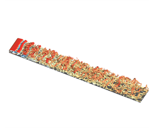
The instantaneous three-dimensional vortical structures are presented in figure 5 for  $G/D=0.1$, $G/D=0.3$ and $G/D=0.9$. In figure 5 $(a)$ for $G/D=0.1$, hardly any vortex structure is observed behind the cylinder until $x/D$ is larger than 10 using $Q$ criterion (Hunt, Wray & Moin Reference Hunt, Wray and Moin1988; Chakraborty, Balachandar & Adrian Reference Chakraborty, Balachandar and Adrian2005) with $Q=0.1$. Vortex shedding is suppressed on both sides of the cylinder due to the thick wall boundary layer and small gap ratio, and there is a large-scale shear layer separating from the cylinder. After $x/D=10$, two-dimensional spanwise vortices resulting from the KH instability of the shear layer are observed. The hairpin-like vortices are initiated behind the KH vortex, which suggests that the KH vortex survives only in a short range. At approximately $x/D=20$, hairpin vortices begin to take shape in the boundary layer. There are a large number of hairpin vortices with different scales downstream, where the wall boundary layer reaches a turbulent state.
Instantaneous three-dimensional vortical structures visualized by isosurfaces of  $Q=0.1$ for three cases, coloured with the instantaneous streamwise velocity $u/U_0$. Results are shown for $(a)$
$(a)$  $G/D=0.1$, $(b)$
$(b)$  $G/D=0.3$, $(c)$
$(c)$  $G/D=0.9$. (The following acronyms are applied: RU – upper roller, SV – secondary vortex.)

The instantaneous vortical structures behind the cylinder for  $G/D=0.3$ shown in figure 5 $(b)$ are substantially different from those for $G/D=0.1$. The shear layer behind the cylinder rolls up and forms vortices shedding from the cylinder. The spanwise roller exhibits good two dimensionality from the upper shear layer marked RU, while the roller (marked RL) from the lower shear layer is covered by the upper roller and braid vortices. There are braid vortices formed behind the upper roller, which has been reported in the numerical study of Ovchinnikov et al. (Reference Ovchinnikov, Piomelli and Choudhari2006) for large gap ratios but has not been reported in experimental studies. It is due to the hot wires and two-dimensional PIV-based experiments are unable to capture these streamwise vortices. These braid vortices are typical structures in flow around an isolated circular cylinder (Williamson Reference Williamson1996a,Reference Williamsonb; Jiang & Cheng Reference Jiang and Cheng2020) and every two adjacent braid vortices with opposite signs usually form a streamwise vortex pair. It should be noted that the braid vortices originate from rollers that are different from the streamwise vortices in the turbulent boundary layer. Hairpin-like vortices are gradually formed at approximately $x/D=10$ and then numerous hairpin vortices are developed behind. Similar to the case of $G/D=0.1$, the flow becomes fully turbulent downstream.
Figure 5 $(c)$ presents the instantaneous three-dimensional vortical structures at $G/D=0.9$. It can be seen that the upper roller (marked RU) is shedding from the upper shear layer, meanwhile, the secondary vortex (marked SV) is found near the wall. Note that the rollers develop to three-dimensional structures through mode B instability (Williamson Reference Williamson1996a), and the braid vortices are generated subsequently, which are similar to that in flow past an isolated cylinder. Different from those in the case of $G/D=0.3$, braid vortices bend upwards or downwards due to the weakening of the wall effect. Meanwhile, braid vortices maintain coherence until approximately $x/D=15$. This is similar to the flow around an isolated cylinder. The hairpin-like vortices are not observed in the current perspective as they are hidden under braid vortices. Rich vortical structures located downstream also imply that the wall boundary layer is in a turbulent state.
3.1.2. Interaction between cylinder wake and secondary vortices
When the gap ratio is large, the wake of the cylinder will have induced effects on the secondary vortices rather than interacting with them directly (Pan et al. Reference Pan, Wang, Zhang and Feng2008; Mandal & Dey Reference Mandal and Dey2011; He et al. Reference He, Wang and Pan2013b, Reference He, Wang, Pan, Feng, Gao and Rinoshika2017). On the contrary, there are direct interactions between the wake vortices and secondary vortices at small gap ratios (Sarkar & Sarkar Reference Sarkar and Sarkar2009, Reference Sarkar and Sarkar2010). The complex vortex interactions can be revealed from the instantaneous flow fields. Figures 6 and 7 illustrate the interaction process for  $G/D=0.3$ and $G/D=0.9$, respectively. The secondary vortices in the case of $G/D=0.1$ are much weaker due to the weak gap flow, so they are not shown here. The secondary vortices are generated in the near-wall region and covered by rollers and braid vortices, therefore, the interactions are shown with tailored three-dimensional vortical isosurfaces with two vertical slices. The instantaneous vortex structures are extracted by $Q$ criterion ( $Q=0.1$) and coloured with streamwise velocity. At the two slices, the isosurface of $Q$ is coloured by spanwise vorticity.
Interactions between secondary vortices and vortex street visualized by three-dimensional vortical isosurfaces of  $Q=0.1$ coloured with the instantaneous streamwise velocity $u/U_0$, and contours of vortical structures ( $Q>0$) for slices coloured with the instantaneous spanwise vorticity $\omega _z$, when $G/D=0.3$. The slices shown are for $(a)$
$(a)$  $z/D={\rm \pi}$, $x/D=2.9$, $t=t_0$; $(b)$
$(b)$  $z/D={\rm \pi}$, $x/D=3.85$, $t=t_0+\Delta t$; $(c)$
$(c)$  $z/D={\rm \pi}$, $x/D=5.65$, $t=t_0+2\Delta t$; where $\Delta t = 1.5D/U_0$. (The following acronyms are applied: RU – upper roller, RL – lower roller, TV – tertiary vortex, SV – secondary vortex.)

Interactions between secondary vortices and vortex street visualized by three-dimensional vortical isosurfaces of  $Q=0.1$ coloured with the instantaneous streamwise velocity $u/U_0$, and contours of vortical structures ( $Q>0$) for slices coloured with the instantaneous spanwise vorticity $\omega _z$, when $G/D=0.9$. The slices shown are for $(a)$
$(a)$  $z/D={\rm \pi}$, $x/D=2.85$, $t=t_0$; $(b)$
$(b)$  $z/D={\rm \pi}$, $x/D=3.60$, $t=t_0+\Delta t$; $(c)$
$(c)$  $z/D={\rm \pi}$, $x/D=4.40$, $t=t_0+2\Delta t$; where $\Delta t = 1.5D/U_0$. (The following acronyms are applied: RU – upper roller, RL – lower roller, TV – tertiary vortex, SV – secondary vortex.)

In figure 6 $(a)$ for $G/D=0.3$, the upper roller (marked RU) has already shed off while the lower roller (marked RL) has raised and is shedding off when $t=t_0$, which lead to obvious asymmetry of the wake and induce the secondary vortex (marked $SV_1$) below the lower roller to lift away from the wall. It should be noted that the secondary vortex rolls up from the separated boundary layer pairing with the lower shear layer. Furthermore, another vortex can be observed aside $SV_1$, which is denoted as the tertiary vortex (marked TV). At $t=t_0$, the upper roller, lower roller and $SV_1$ exhibit good two dimensionality, especially $SV_1$. When $t=t_0+\Delta t$, shown in figure 6 $(b)$, the lower roller and $SV_1$ have moved up together towards the upper roller and are interacting with each other. During the interaction process, the lower roller is stretched severely into a thin structure while the upper roller maintains its vortical shape. Meanwhile, the secondary vortex ( $SV_1$) has been split into two parts, one of which is $ASV_1$ and the other is $BSV_1$. Here $BSV_1$ is left over with a lower streamwise velocity than $ASV_1$, just as $BSV_0$, shown in figure 6 $(a)$, is left over from a previous secondary vortex. The $ASV_1$ rotates with $BSV_0$ and the upper roller then merges with each vortex. Meanwhile, a new secondary vortex (marked $SV_2$) has been formed near the wall. At $t=t_0+2\Delta t$, as shown in figure 6 $(c)$, the lower roller disappears, indicating that the lower roller has broken down and lost its coherence. This is consistent with the results observed by Sarkar & Sarkar (Reference Sarkar and Sarkar2009) for $G/D=0.25$, $0.5$ and Zhou et al. (Reference Zhou, Qiu, Li and Liu2021) for $G/D=0.5$. He et al. (Reference He, Wang, Pan, Feng, Gao and Rinoshika2017) claim that the breakdown of the lower roller is similar to the ’vortex tearing’ (Moore & Saffman Reference Moore and Saffman1975) for $G/D=0.5$. Here the upper roller, $ASV_1$ and $BSV_0$ with the same rotational direction show vortex merging. It is worth noting that this vortex split and merging process were barely observed in previous studies. Although the flow with a similar gap ratio ( $G/D=0.25$) has been researched by Sarkar & Sarkar (Reference Sarkar and Sarkar2009), their vorticity plot of an instantaneous flow field can hardly distinguish the vorticity of two same-signed vortices and the wall boundary shear.
Figure 7 shows the vortex interactions for  $G/D=0.9$. The upper rollers, lower rollers and secondary vortices still exist at this gap ratio. Both the upper roller (marked $RU_1$) and lower roller (marked $RL_1$) have shed off as illustrated in figure 7 $(a)$ at $t=t_0$. The vortex pair is symmetric about the centreline of the cylinder, which is different from that in the $G/D=0.3$ case and similar to the flow around an isolated cylinder. The secondary vortex $SV_1$ also exhibits good two dimensionality. Meanwhile, it can be observed that the distance between $RL_1$ and $SV_1$ is much larger than that in $G/D=0.3$, as $SV_1$ sheds off earlier than $RL_1$ in this case. When the flow evolves to $t=t_0+\Delta t$, as shown in figure 7 $(b)$, the lower roller $RL_1$ is convected along the streamwise direction and gets less stretched, and the secondary vortex $SV_1$ descends to a lower height, compared with those for $G/D=0.3$. The upper roller $RU_1$ does not interact with the secondary vortex $SV_1$ but moves away from it, which agrees with the results of He et al. (Reference He, Wang, Pan, Feng, Gao and Rinoshika2017) and Zhou et al. (Reference Zhou, Qiu, Li and Liu2021). At the same time, a new secondary vortex $SV_2$, as well as a small tertiary vortex (marked TV), are generated near the wall. When $t= t_0+2\Delta t$, the direct interaction between $SV_2$ and $RL_1$ can be observed in figure 7 $(c)$. As the lower roller $RL_1$ is stronger, a large portion of the secondary vortex is induced to lift away from the wall while another portion is stretched in the streamwise direction near the wall. At this moment, $SV_1$ is broken into several segments in the spanwise direction. Actually, the secondary vortex is induced to evolve into several hairpin-like vortices as depicted in § 3.1.3. The above vortex dynamic verifies the experimental observations from He et al. (Reference He, Pan and Wang2013a) that the secondary vortices can be either entrained into the wake or pushed down towards the wall at $G/D=1.0$. It is speculated that portions of the secondary vortex entrained into the wake develop to the heads of the hairpin-like vortices and those pushed down towards the wall form the legs of the hairpin-like vortices.
The appearance of the tertiary vortex along with the secondary vortex is interesting, which has not been noticed in previous studies in cylinder wake-induced transition processes above a flat plate. Figure 8 shows the close-up view of the instantaneous tertiary vortex. It can be found that the tertiary vortex generation is similar for  $G/D=0.3$ and $G/D=0.9$. The tertiary vortex is induced by the lifting-up $SV_1$ and rotates in the opposite direction to $SV_1$. However, the tertiary vortex is much weaker than the secondary vortex in strength due to the squeezing of two secondary vortices ( $SV_1$ and $SV_2$). Thus, the two dimensionality of the tertiary vortex in the spanwise direction is not maintained, especially at $G/D=0.3$ shown in figure 8 $(a)$. Note that although the tertiary vortex is periodically generated with the secondary vortex, it is unable to survive for a long time. When $SV_2$ develops downstream, the tertiary vortex disappears rapidly because of its weak strength.
Close-up view of instantaneous secondary vortex and tertiary vortex coloured with spanwise vorticity. The slices show the contours of instantaneous spanwise vorticity with the superimposition of streamlines at  $z/D=0$. Results are shown for $(a)$
$(a)$  $G/D=0.3$, $Q=0.1$ and $0.01$; $(b)$
$(b)$  $G/D=0.9$, $Q=0.1$. (The following acronyms are applied: RU – upper roller, RL – lower roller, TV – tertiary vortex, SV – secondary vortex.)

3.1.3. Hairpin vortices generation
The hairpin vortices are the important structures in the turbulent boundary layer. However, the generation of hairpin vortices in the present configuration is rarely reported. The relevant study has been conducted at large gap ratios (Pan et al. Reference Pan, Wang, Zhang and Feng2008; He et al. Reference He, Wang and Pan2013b, Reference He, Pan, Feng, Gao and Wang2016). In the present study it is found that hairpin vortices are generated via different mechanisms for different small gap ratios.
Figure 9 illustrates the generation process of hairpin vortices for  $G/D=0.1$, which is divided into several stages. The first stage is shown in figure 9 $(a)$, the KH vortex as the two-dimensional spanwise roller has been formed due to the KH instability of the shear layer. The non-uniformity appearance of this KH vortex implies the three-dimensional instability of the roller. In the second stage, shown in figure 9 $(b)$, the KH vortex is reattaching. The uneven distribution of the streamwise velocity along the KH roller is enhanced by the strong shear due to the large velocity difference between the upper and lower sides of the vortex. As shown in figure 9 $(c)$, the KH vortex is broken in the third stage. Due to the strong shear effect, the high momentum parts form into the heads of the hairpin-like vortices and the low momentum parts develop into the legs of these hairpin-like vortices. The background mean shear makes the flow acceleration coupled with lift-up motion. In the fourth stage, shown in figure 9 $(d)$, the downstream high momentum heads lift to be accelerated, while the upstream low momentum legs are still retarded near the wall. Therefore, these hairpin-like vortices keep stretching in this stage. The stretching of hairpin-like vortices helps to form hairpin vortices presented in figure 9 $(e)$. Note that there are two different interactions between the vortices. One is the interaction between hairpin-like vortices and the other is the interaction caused by the high-speed part of the upstream vortices catching up with the low-speed part of the downstream vortices. Both of these interactions result in hairpin-like vortices breaking down into several small-scale structures, which can be observed in figure 9 $(e)$. A similar generation process of hairpin vortices from the KH vortices was also identified by Dubief & Delcayre (Reference Dubief and Delcayre2000) in a backward-facing step flow.
The generation process of hairpin vortices visualized by isosurfaces of  $Q=0.1$ for $G/D=0.1$, coloured with the instantaneous streamwise velocity $u/U_0$. Results are shown for $(a)$
$(a)$  $t=t_0$; $(b)$
$(b)$  $t=t_0+3\Delta t$; $(c)$
$(c)$  $t=t_0+5\Delta t$; $(d)$
$(d)$  $t=t_0+7\Delta t$; $(e)$
$(e)$  $t=t_0+11\Delta t$, where $\Delta t = D/U_0$.

In figure 10 the generation process of hairpin vortices for  $G/D=0.3$ is presented. Following the vortex dynamics shown in figure 6, when the the upper roller, $ASV_1$ and $BSV_O$ with the same rotational direction have completed vortex merging, $BSV_1$ can still be observed, as shown in figure 10 $(a)$. Some braid vortices bend downwards while the others bend upwards, which suggests the three-dimensional instability of the merged vortex. Owing to the mean shear, braid vortices keep stretching as shown in figure 10 $(b)$. Furthermore, the downstream neck originating from the merged vortex, which connects two braid vortices bending upwards, lifts up to be accelerated and develops into the head of the hairpin-like vortex. Meanwhile, the upstream braid vortices have evolved into the legs of the hairpin-like vortex. The neck that connects the two braid vortices bending downwards lifts. Moreover, the hairpin vortices form from hairpin-like vortices through the vortex-stretching mechanism. In figure 10 $(c)$ there are a large number of hairpin vortices formed as the streamwise vortices (the legs of the hairpin vortices) continue to be stretched. Note that under the braid vortices, there are several new hairpin-like vortices, which may develop from the other parts of the merged vortical structures.
The generation process of hairpin vortices visualized by isosurfaces of  $Q=0.1$ for $G/D=0.3$, coloured with the instantaneous streamwise velocity $u/U_0$. The structures marked by the dotted line are the hairpin-like vortices or hairpin vortices. Results are shown for $(a)$
$(a)$  $t=t_0$; $(b)$
$(b)$  $t=t_0+2\Delta t$; $(c)$
$(c)$  $t=t_0+4\Delta t$, where $\Delta t = D/U_0$.

For the case of  $G/D=0.9$, there are enough spaces for the rollers and braid vortices to develop normally as with those in the flow around a cylinder for large gap ratios or an isolated cylinder. Considering the hairpin vortex is generated from the secondary vortex when $G/D$ is equal to 1.0 (He et al. Reference He, Pan and Wang2013a), the secondary vortex dynamics should be taken into account for the present $G/D=0.9$ case. However, the secondary vortices are covered by the braid vortices as shown in figure 5 $(c)$, the evolution of the secondary vortex is hard to be displayed directly. Alternatively, the clustering method (Jiménez, Del Álamo & Flores Reference Jiménez, Del Álamo and Flores2004; Dong et al. Reference Dong, Huang, Yuan and Lozano-Durán2020) is adopted to extract the secondary vortex, as illustrated in figure 11. As it has been depicted in figure 7, the newly generated secondary vortex exhibits good two dimensionality. As it evolves downstream, the secondary vortex shown in figure 11 $(a)$ is disturbed, and the streamwise velocity distribution is uneven. Due to the interaction between the secondary vortex and the lower roller, the secondary vortex is stretched in the streamwise direction, as shown in 11 $(b)$. Notably, the low momentum parts near the wall are retarded and evolve into the legs of the hairpin-like vortices, while the high momentum parts at the top develop into the heads of the hairpin-like vortices as shown in figure 11 $(c)$. On account of the background mean shear, shown in figure 11 $(d)$, the upstream legs are still retarded, whereas the downstream high momentum heads are lifted to be accelerated. The hairpin-like vortices continue stretching with their heads lifting until the wake is encountered, then the heads are entrained by the lower roller and braid vortices from the lower roller. Therefore, hairpin vortices, in this case, do not have complete heads as shown in 11 $(d)$, which confirms the speculation based on the experimental plan view visualization for $G/D=1.0$ from He et al. (Reference He, Pan and Wang2013a). Moreover, it should be noted that the hairpin vortices without complete heads are different than the matured hairpin vortices in the studies of Pan et al. (Reference Pan, Wang, Zhang and Feng2008) for large gap ratios. Since the direct interaction between cylinder wake and wall boundary layer is quite weak for large gap ratios (Pan et al. Reference Pan, Wang, Zhang and Feng2008; Mandal & Dey Reference Mandal and Dey2011; He et al. Reference He, Wang and Pan2013b, Reference He, Pan, Feng, Gao and Wang2016), the hairpin vortices developed from the secondary vortex are less affected by the wake.
The generation process of hairpin vortices visualized by isosurfaces of  $Q=0.1$ for $G/D=0.9$, coloured with the instantaneous streamwise velocity $u/U_0$. The structures marked by the dotted line are the hairpin-like vortices or hairpin vortices. Results are shown for $(a)$
$(a)$  $t=t_0$; $(b)$
$(b)$  $t=t_0+0.5\Delta t$; $(c)$
$(c)$  $t=t_0+1.0\Delta t$; $(d)$
$(d)$  $t=t_0+1.5\Delta t$, where $\Delta t = D/U_0$.

3.2. Transition to turbulence
The wall boundary layer transition can be induced by the wake of the cylinder at large gap ratios (Ovchinnikov et al. Reference Ovchinnikov, Piomelli and Choudhari2006; Pan et al. Reference Pan, Wang, Zhang and Feng2008; Mandal & Dey Reference Mandal and Dey2011; He et al. Reference He, Wang and Pan2013b, Reference He, Pan, Feng, Gao and Wang2016). In the present small gap ratio situations, the development of a turbulent boundary layer downstream behind reattachment is explored as well. The streamwise evolution of the averaged streamwise velocity profile and the disturbance growth inside the boundary layer are analysed to interpret the wall boundary layer transition.
3.2.1. Boundary layer profiles and shape factor
The time- and spanwise-averaged streamwise velocity profiles  $U/U_0$ at several typical streamwise locations are illustrated in figure 12 for $G/D=0.1$, $G/D=0.3$ and $G/D=0.9$. The velocity profiles are compared with the Blasius boundary layer profile. A prominent velocity profile deficit can be observed behind the cylinder (at $x/D=1$) for all the gap ratios. With the increase of the gap ratio, the velocity overshoot is more obvious on both sides of the deficit region because of the intensifying gap flow. The velocity overshoot diminishes along the streamwise direction, and the diminished speed is quicker at a larger gap ratio. The wake-like profile gradually evolves to a boundary-layer-like profile. The velocity profiles increase from the wall monotonically. Meanwhile, the deviation of the boundary layer profiles from the Blasius profile is obvious. The near-wall velocity profiles become blunter, suggesting that the wall boundary layers evolve to turbulence.
Time- and spanwise-averaged velocity profiles at different streamwise locations:  $(a)$
$(a)$  $G/D=0.1$, $(b)$
$(b)$  $G/D=0.3$, $(c)$
$(c)$  $G/D=0.9$. The red full lines represent the Blasius profiles. The black line represents $U/U_0=0$.

To further characterize the wall boundary layer transition, the shape factor  $H$, as a useful indicator for the laminar-to-turbulent transition, is calculated as
 \begin{equation} H= \frac{\delta^{*}}{\theta}, \end{equation}
where  $\delta ^{*}$ and $\theta$ are displacement thickness and momentum thickness, respectively, with the following definitions:
 \begin{equation} \delta^{*}=\int_0^{\delta} \left(1-\frac{U}{U_{\delta}}\right){{\rm d} y}, \quad \theta=\int_{0}^{\delta} \frac{U}{U_{\delta}}\left(1-\frac{U}{U_{\delta}}\right){{\rm d} y}. \end{equation}
Here  $\delta$ is the boundary layer thickness. Similar to Sarkar & Sarkar (Reference Sarkar and Sarkar2009) and He et al. (Reference He, Wang and Pan2013b), the boundary layer edge is indicated using the height of the local maximum of $U/U_0$ between the wall and the wake deficit region. If the local maximum is absent, the boundary layer edge will be determined by the standard boundary layer assumption (the velocity at the boundary layer edge equals $0.99U_0$). For the laminar Blasius boundary layer, the shape factor $H=2.59$, whereas the value is $H=1.4$ for a zero pressure gradients turbulent boundary layer. The evolution of the shape factor $H$ is plotted in figure 13. It is observed that $H$ is larger than 2.59 at the near-wake region due to the complex interactions and the accelerated gap flow (Wang & Wang Reference Wang and Wang2021), while $H$ is close to 1.4 at the far downstream indicating a fully turbulent boundary layer is developed.
Shape factor of the wall boundary layer for different gap ratios. The shape factor of the turbulent boundary layer with zero pressure gradients ( $H=1.4$) and laminar Blasius boundary layer ( $H=2.59$) are provided in back dashed lines for reference.

3.2.2. Disturbance growth inside the boundary layer
To further understand the mechanism of wall boundary layer transition in the present small gap ratio situation, the disturbance growth inside the boundary layer is studied in this section. Firstly, the profiles of streamwise velocity fluctuation at several typical streamwise locations are shown in figure 14. These streamwise locations are chosen from the pre-transitional zone, transitional zone and turbulent zone, and are plotted in figures 14 $(a)$, 14 $(b)$ and 14 $(c)$, respectively. These three zones are identified by the streamwise velocity profiles (figure 12), the shape factor (figure 13) and the spanwise-averaged streamwise velocity fluctuation intensity (figure 14). In the pre-transitional zone the direct wake/boundary layer interaction results in only one peak, as illustrated in figure 14 $(a)$. There is only one apparent peak appearing inside the boundary layer due to the strong interactions between the wake and wall boundary layer. It is easy to distinguish the fluctuation from the wake or the instability of the boundary layer for large $G/D$ (Ovchinnikov et al. Reference Ovchinnikov, Piomelli and Choudhari2006; Mandal & Dey Reference Mandal and Dey2011; He et al. Reference He, Wang and Pan2013b). The black full curve is obtained by optimal disturbance theory from Luchini (Reference Luchini2000), with which the disturbance distributions of FST induced bypass transition from the experiment of (Matsubara & Alfredsson Reference Matsubara and Alfredsson2001) are in accordance. Ovchinnikov et al. (Reference Ovchinnikov, Piomelli and Choudhari2006), Mandal & Dey (Reference Mandal and Dey2011) and He et al. (Reference He, Wang and Pan2013b) found that the $u'_{rms}$ profiles in the pre-transitional boundary layer show self-similarity for large gap ratios, and the $u'_{rms}$ profiles are in agreement with the theory. The self-similarity in $u'_{rms}$ profiles is observed in the pre-transitional zone in the present cases, however, they are deviated from the optimal disturbance theory due to the direct interaction between the boundary layer and the emerged wake at small gap ratios.
Profiles of the spanwise-averaged streamwise velocity fluctuation intensity normalized by the maximum value of  $u'_{rms}$ at different streamwise locations. In the $(a)$ pre-transitional zone, $(b)$ transitional zone, $(c)$ turbulent zone. The height in the wall-normal direction is normalized by $\delta ^{*}$. The location of the boundary layer is located by hexagon makers. The black full curve in $(a)$ is the optimal disturbance growth theory from Luchini (Reference Luchini2000). From left to right, data are from the case $G/D=0.1$, $G/D=0.3$ and $G/D=0.9$, respectively.

Further downstream, a second  $u'_{rms}$ peak gradually appears inside the boundary layer, as shown in figure 14 $(b)$, implying the occurrence of a boundary layer transition. When the second $u'_{rms}$ peak dominates, the flow is regarded as a turbulent boundary layer. This is consistent with the observation in figure 12, where the streamwise velocity profile develops towards the turbulent type. Furthermore, due to the existence of the inner fluctuation peak, there is an inflexion point located between this peak and the disturbance region, which is attributed to the sheltering effect in the near-wall region by strong mean shear (Hunt & Durbin Reference Hunt and Durbin1999; Jacobs & Durbin Reference Jacobs and Durbin2001). The envelope of the inner fluctuation peaks forms a sheltering edge. Low-frequency disturbances are selected to penetrate the sheltering edge to generate streaks (Wang, Mao & Zaki Reference Wang, Mao and Zaki2019). The visualizations in figure 15 show that the streaks are generated where the transition of the boundary layer occurs. Recalling that the generation of hairpin vortices is accompanied by the emergence of many streamwise vortices, such vortical disturbances can effectively perturb the boundary to generate streaks through the lift-up mechanism (Zaki & Saha Reference Zaki and Saha2009; Monokrousos et al. Reference Monokrousos, Åkervik, Brandt and Henningson2010). Thus, although the near-wake dynamics is diverse for the studied small gap ratios, the transitions to turbulence downstream follow the route of bypass transition (Jacobs & Durbin Reference Jacobs and Durbin2001; Zaki Reference Zaki2013). In the small gap ratios the wake/boundary layer interaction alters the perturbation quantitatively and deviates from the theoretical profiles, which is different from the large gap ratios.
Instantaneous streamwise velocity fluctuations in  $x$–
$x$– $z$ plane. Results are shown for $(a)$
$(a)$  $G/D=0.1$, $y/D=0.1$; $(b)$
$(b)$  $G/D=0.3$, $y/D=0.15$; $(c)$
$(c)$  $G/D=0.9$, $y/D=0.15$.

As the boundary layers develop into turbulence, as shown in figure 14 $(c)$, there is only one peak located inside the boundary layer, and the peak resulting from the wake has decayed. The $u'_{rms}$ profiles show that a great self-similarity is achieved in the turbulent zone. Figure 15 shows that the streaks exist in both the transitional zone and turbulent zone, which may be related to self-sustaining mechanisms. Figure 16 presents the streamwise velocity profiles of the turbulent boundary layer. Close to the wall, the profiles agree very well with $U^+=y^+$. In the outer region the turbulent log region has been developed. It should be noted that the streamwise location, where the logarithmic layer has been found, is $x/D=45$ for present small gap ratios. However, for large gap ratios, He et al. (Reference He, Pan, Feng, Gao and Wang2016) did not observe the logarithmic layer at $x/D=50$ for $G/D=2.0$ and Ovchinnikov et al. (Reference Ovchinnikov, Piomelli and Choudhari2006) did not find this region until $x/D=70$ for $G/D=3.5$. Therefore, it can be corroborated that a turbulent equilibrium is established more quickly for small gap ratios than for large gap ratios.
Mean boundary layer profile at  $x/D=45$. The log-law expression used here is $U^+=1/0.41\ln (y^+)+4.6$ (the inclined straight line). The dashed curve is $U^+=y^+$.

In order to characterize the growth of the whole disturbance level inside the boundary layer along the streamwise direction, the averaged boundary layer disturbance energy  $E_{rms}$ ( $E_{rms}=\int _0^{\delta _s} [(u'_{rms})^2+(v'_{rms})^2+(w'_{rms})^2]\,{{\rm d} y}/(U^2_0 \delta _s)$) is employed as a measure, where $\delta _s$ is the sheltering edge. The integral upper limit is set to $\delta _s$ instead of $\delta$ to exclude the contribution of wake disturbance. Note that the sheltering edge does not exist in the pre-transitional zone in this study, the $\delta ^*$ is used as the integral upper limit. Actually, $\delta ^*$ is very close to $\delta _s$. The variation of $E_{rms}$ as a function of streamwise location $x$ is plotted in figure 17. There are two exponential growth zones in the pre-transitional stage for all the cases. The spatial growth rate of $E_{rms}$ in the first zones are all larger than the spatial growth rate in the second zones. After $E_{rms}$ reaches a maximum and saturates, its level gradually declines. It is attributed to the decaying characteristics of the outside wake, which leads to a significant weakening of the interaction between the wake and the boundary layer. Recalling the evolutions of the KH vortex (figure 9 for $G/D=0.1$) and secondary vortex (figures 6 and 10 for $G/D=0.3$, figures 7 and 11 for $G/D=0.9$), it is inferred that the forceful formation of the KH vortex (for $G/D=0.1$) or secondary vortex (for $G/D=0.3$ and $G/D=0.9$) leads to the first growth, while the three-dimensional destabilization of the KH vortex or secondary vortex is the reason for the second growth. The three-dimensional instabilities result in redistribution and nonlinear saturation of the disturbance energy $E_{rms}$. He et al. (Reference He, Wang and Pan2013b) also found a two stage growth of $E_{rms}$ in experimental results for $G/D=1.8$, but they did not observe streak structure. Ovchinnikov et al. (Reference Ovchinnikov, Piomelli and Choudhari2006) and Mandal & Dey (Reference Mandal and Dey2011) evaluated the disturbance energy for large gap ratios ( $G/D=3.5$ and $G/D=3$, 3.5, 4) and found that the transition is similar to FST induced bypass transition. Note that the growth in $E_{rms}$ in the present small gap ratios is different from that for the FST induced bypass transition in the boundary layer. In the bypass transition the disturbance level is low in the pre-algebraic-growth stage due to the receptivity process while it grows algebraically after this stage (Fransson, Matsubara & Alfredsson Reference Fransson, Matsubara and Alfredsson2005). It is the algebraic growth of disturbances that give rise to streaks (Matsubara & Alfredsson Reference Matsubara and Alfredsson2001). However, the formation of the streaks in the present studies is located downstream of the saturation state, where the disturbance level has declined.
The streamwise growths of the disturbance energies inside the boundary layer. The purple, black and red lines denote the exponential fittings.

3.2.3. Power spectral density of streamwise velocity fluctuations
In order to investigate the frequency of disturbance, the power spectral density map is applied here for  $G/D=0.3$ as the typical case shown in figure 18. The signals are extracted from three lines with different wall-normal heights in the $z/D={\rm \pi}$ plane. From figure 18 $(a)$ it can be seen that the high-frequency disturbance ( $St_H$) is dominant at $y/D=1.3$, while the low-frequency ( $St_L$) disturbance is stronger at $y/D=0.1$. The enlarged high-frequency regions are shown in 18 $(b)$. It can be observed that there are strong high-frequency peaks for $2.8\leqslant x/D \leqslant 4$ at $y/D=1.3$, which is due to the shedding of the upper rollers. However, the peaks after $x/D=4$ are significantly weakened and disappear after about $x/D=7$ because the upper rollers lose their two dimensionality and decay. For $y/D=0.8$, the strong peaks appear more upstream than those at $y/D=1.3$ and only exist in a very small streamwise region, which is attributed to the lifted lower rollers being under severe stretching during the interaction process (see figure 6). For $y/D=0.1$, the high-frequency peaks in the range of $2\leqslant x/D \leqslant 4$, where the secondary vortices are formed and lifted. The result suggests that the shedding of the secondary vortices is weaker than that of the upper and lower rollers. The enlarged low-frequency regions are shown in figure 18 $(c)$. The peaks of $St_L$ can be found from $x/D=5$ to $x/D=10$ at $y/D=1.3$. Considering the visualization of the spanwise vortex in figure 10, it is speculated that the three-dimensionality destabilization of the spanwise vortices results in the low-frequency signals. Due to reattachment of the streamwise vortices, the low-frequency signals disappear at $y/D=1.3$ and $x/D=10$ while they appear at $y/D=0.1$. At $y/D=0.8$, the low-frequency signal can always be captured along the streamwise direction, which suggests that the spectrum shifts towards low frequencies due to the growth of the streaks. This observation is consistent with that in the studies of Ovchinnikov et al. (Reference Ovchinnikov, Piomelli and Choudhari2006) for large gap ratios. The low-frequency signal reappears at about $x/D=12$ for $y/D=1.3$. It could be the further lifted hairpin vortices along with the instability of low-speed streaks that generate new hairpin vortices. Then, the hairpin packets may be formed in the boundary layer occupied by the streaks, which are the keys of a self-sustained turbulent boundary layer. $(a)$ Power spectral density map of streamwise velocity fluctuations along different lines from $z/D={\rm \pi}$ slice when $G/D=0.3$, which is normalized by the maximum value of all points. $(b)$ Enlarged high-frequency parts in the blue box of panel $(a)$, which are not normalized. $(c)$ Enlarged low-frequency parts in the black box of panel $(a)$, which are normalized by the maximum value of the local point. From left to right, data are from the line $y/D=1.3$, $y/D=0.8$ and $y/D=0.1$, respectively.

3.3. Dynamic mode decomposition analysis
Dynamic mode decomposition (DMD) is a widely used tool to identify the important dynamics embedded in time-sequential data from an unsteady flow field Schmid (Reference Schmid2010). Dynamic mode decomposition extracts a set of modes from the original unsteady dynamic system. Each of these modes is associated with a single frequency as well as the corresponding spatial structures. Dynamic mode decomposition is employed to extract the dominant modes and corresponding topology structures to help understand the flow dynamics.
The snapshots of the flow fields can be decomposed as
 \begin{equation} \varPhi(\boldsymbol{x},t)=\boldsymbol{U}(\boldsymbol{x})+\sum_{k=1}^{r}b_k\phi_k(\boldsymbol{x}) {\rm e}^{\omega_k t}, \end{equation}
where  $\boldsymbol {U}$, $\varPhi$, $\phi _k$ and $b_k$ are the mean field, reconstructed field, $k$th DMD mode and the magnitude of the $k$th DMD mode, respectively. Here $\omega _k$ is obtained by $\omega _k=\log (\mu _k)/\Delta t$, where $\mu _k$ is the eigenvalue of the $k$th mode. In the present study the DMD analysis is based on 500 snapshots of the three-dimensional flow fields. Each sample consists of the three velocity components $u, v, w$. The three-dimensional snapshots are sampled over a time span of 37, 72 and 66 vortex shedding periods for $G/D=0.1$, $G/D=0.3$ and $G/D=0.9$, respectively. The time interval between the snapshots is set to be $\Delta U_0/D=0.5$, which corresponds to a sampling frequency that is 13.5, 6.9 and 7.6 times the frequency of vortex shedding for $G/D=0.1$, $G/D=0.3$ and $G/D=0.9$, respectively. In order to capture the key regions of the wake/boundary layer interaction, the spatial region over which the data is extracted covers $9\leqslant x/D\leqslant 30$ for $G/D=0.1$, $-1\leqslant x/D\leqslant 20$ for $G/D=0.3$ and $G/D=0.9$. The convergence of the field samples was verified by repeating DMD using 400 snapshots.
The spectrum of the DMD modes for  $G/D=0.3$ as the typical case is shown in figure 19 $(a)$. The dimensionless frequency (Strouhal number, $St$) is normalized by the dimensionless characteristic frequency of vortex shedding ( $St_0=0.289$) for $G/D=0.3$, while the magnitude $|b|$ is normalized by the maximum value $|b|_{max}$. In the DMD spectrum the predominant frequency is identified as $St/St_0=1$, which indicates that the vortex shedding frequency is the characteristic frequency within the chosen flow field region. The corresponding mode, marked $\phi _1$, is also termed the high-frequency mode. The mode with the second largest amplitude has very low frequency, marked $\phi _2$, which is termed the low-frequency mode. These two modes are the main dynamic modes. The power spectrum densities of the corresponding mode coefficients are shown in figure 19 $(b)$, which present distinct peaks at $St_L=0.0274St_0$ and $St_H=St_0$ demonstrating the ability of orthogonalizing the temporal dynamics from DMD. $(a)$ Spectrum of the DMD modes with positive frequency when $G/D=0.3$. Here $St_0=0.289$ is the Strouhal number of the case $G/D=0.3$; $\phi _1$ and $\phi _2$ are the selected high- and low-frequency modes, respectively. $(b)$ Power spectrum density of DMD mode coefficient.

Figure 20 $(a)$ shows the topology of the high-frequency DMD mode $\phi _1$ for $G/D=0.3$. It is clear that this mode is dominated by the alternating structures separated in the streamwise direction with the highly regular arrangement, which shows that this mode with predominant frequency $St_H$ captures the coherent structures of the rollers (Kármán vortices) in the wake. In the upstream these structures exhibit great coherence in the spanwise direction, while presenting three-dimensional features in the form of spanwise wrinkles and disappearing gradually downstream. This process implies the three-dimensional destabilization of the rollers in the downstream evolution, which is consistent with the observation above. The structures associated with the secondary vortex and the tertiary vortex are extracted from the near-wall region shown in the box at the top right corner in figure 20 $(a)$. The red structure corresponds to the secondary vortex split into two parts as shown in figure 6. While the blue structure corresponds to the tertiary vortex lying on the wall.
Isosurfaces of the real part of DMD modes. The red parts are positive and the blue parts are negative.  $(a)$ The high-frequency DMD mode $\phi _1$, the arrow points to the structures extracted near the wall. $(b)$ The low-frequency DMD mode $\phi _2$. (The following acronyms are applied: TV – tertiary vortex, SV – secondary vortex.)

The topology of the low-frequency DMD mode  $\phi _2$ is shown in figure 20 $(b)$, of which the significant characteristic is the highly elongated streamwise structures. In contrast to the high-frequency mode $\phi _1$, the low-frequency mode initiates and persists inside the boundary layer. The positive/negative structures for this mode alternate in the spanwise direction. The low-frequency mode $\phi _2$ is associated with the generation of streaks inside the boundary layer.
The DMD modes for  $G/D=0.1$ and $(G/D=0.9)$ are not shown as they are similar to those in the case of $G/D=0.3$. The flow reconstruction with the dominant modes can help us to understand flow dynamics. The instantaneous three-dimensional vortical structures reconstructed by the corresponding high-frequency mode are given in figure 21. The isosurface of $Q=0.1$ in figure 21( $a$–
$a$– $c$) is coloured with the instantaneous spanwise vorticity. It can be observed for all three cases that the spanwise vortices with good two dimensionality present three-dimensional features as they evolve downstream. As shown in figure 21 $(a)$ for $G/D=0.1$, the KH vortex loses stability after $x/D=12$. For $G/D=0.3$, an upper roller (marked RU) has shed off while the lower roller (marked RL) is shedding, as shown in figure 21 $(b)$. The second vortex (marked SV) is lifting up with the same rotational direction as the upper roller. There is only one roller downstream of the secondary vortex and the upper roller, which suggests the merging of the secondary vortex and the upper roller. It should be noted that the raised lower roller pairs with the secondary vortex, as shown in figure 6, and induces the secondary vortex to lift away from the wall. Therefore, the role of the lower roller should not be neglected in the merging of vortices. Although the lower roller has the opposite rotating sense with the upper roller and the secondary vortex, it also takes part in the merging process even if this interaction process results in its annihilation in the end. The merged roller will present three-dimensional features after $x/D=8$. A similar phenomenon is observed in figure 21 $(c)$ for $G/D=0.9$, but the difference is that the secondary vortex is less lifted and the lower roller is convected to a longer streamwise distance. Moreover, the appearance of the secondary vortex and tertiary vortex in mode $\phi _1$, shown in figures 21 $(d)$ and 21 $(e)$, implies that both these vortical structures have the same shedding frequency as the Kármán vortices.
The instantaneous three-dimensional vortical structures reconstructed by corresponding the high-frequency DMD mode, coloured with the instantaneous spanwise vorticity. Results are shown for  $(a)$
$(a)$  $G/D=0.1$, $Q=0.1$; $(b)$
$(b)$  $G/D=0.3$, $Q=0.1$; $(c)$
$(c)$  $G/D=0.9$, $Q=0.1$. Close-up views with $Q=0.01$ for $G/D=0.3$ in $(d)$ and $Q=0.05$ for $G/D=0.9$ in $(e)$. (The following acronyms are applied: RU – upper roller, RL – lower roller, TV – tertiary vortex, SV – secondary vortex.)

4. Conclusion
Direct numerical simulations of the flow around a circular cylinder near a plane wall are performed within the range of  $0.1\leqslant G/D\leqslant 0.9$ ( $Re_D=1000$). The effects of $G/D$ on the three-dimensional vortical structures and wake dynamics are presented. The interactions between the rollers and secondary vortices are investigated from the instantaneous flow fields. Specifically, the mechanisms of the hairpin vortex generations and the transitions induced by the wake are revealed in the current work.
For the vortex dynamics, detailed vortex evolution processes are presented for three typical small gap ratio cases. The KH instability occurs far from the cylinder at  $x/D=10$ for $G/D=0.1$ and results in spanwise KH vortices. The KH vortices evolve into hairpin vortices gradually due to the three-dimensional instability and background mean shear. The vortex dynamics for such small gap ratios have received little attention before. At $G/D=0.3$, the positive lower roller and the secondary vortex raise together toward the negative upper roller and interact with each other, which agrees with previous observations (Sarkar & Sarkar Reference Sarkar and Sarkar2009; He et al. Reference He, Wang, Pan, Feng, Gao and Rinoshika2017; Zhou et al. Reference Zhou, Qiu, Li and Liu2021) at close gap ratios ( $G/D=0.25$ and $G/D=0.5$). However, it is found here that during the interaction, the secondary vortex is split into two parts, which is confirmed by three-dimensional DMD analysis. The upper roller and the secondary vortex rotating in the same direction merge with the assistance of the lower roller inducing the secondary vortex to lift away from the wall, resulting in a clockwise rotating vortex downstream. Although the lower roller has the opposite rotation its participation in vortex merging can not be neglected. This merged vortex develops into hairpin vortices eventually. Meanwhile, a pair of braid vortices from the upper roller with their head connected evolves into a hairpin vortex. When $G/D=0.9$, the process similar to the experimental observation (He et al. Reference He, Wang, Pan, Feng, Gao and Rinoshika2017) at $G/D=1.0$ is that the interaction occurs between the secondary vortex and the lower roller without the upper roller. The evolution of a hairpin vortex from the spanwise secondary vortex under the braid vortices is clearly presented, which is similar to that in the large gap ratio cases (Pan et al. Reference Pan, Wang, Zhang and Feng2008; He et al. Reference He, Wang and Pan2013b, Reference He, Pan, Feng, Gao and Wang2016). However, different from the large gap ratio cases, most of the hairpin vortices are observed without a complete head due to the entrainment of the lower roller and braid vortices from the lower roller. Moreover, it is found that portions of the secondary vortex entrained into the wake are the heads of the hairpin vortices and those pushed down towards the wall form the legs of the hairpin-like vortices, which explains the phenomenon observed in the experiments of He et al. (Reference He, Pan and Wang2013a) at $G/D=1.0$.
During the vortex evolution, the novel tertiary vortex is found. The tertiary vortex is induced by the lifting-up secondary vortex, rotating in the opposite direction to the secondary vortex. The squeezing of two adjacent secondary vortices causes the tertiary vortex to survive for little time. The strength and continuity of the tertiary vortex are both worse than those of the secondary vortex, especially at  $G/D=0.3$. Furthermore, the DMD analysis corroborates that the tertiary vortex has the same characteristic frequency along with the secondary vortex as the Kármán vortices.
The wake-induced transition at small gap ratios has been barely noticed. It is revealed in the current work that the transition route is similar for all the small gap cases studied. In the pre-transitional region the streamwise velocity fluctuations deviate from the optimal growth theory, which is different from that in the large gap ratio flows. In the transitional region the sheltering effect of the boundary layer to external disturbance plays a significant role. The low-frequency disturbances are selected to penetrate the sheltering edge to generate streaks, which is also corroborated by DMD analysis. Meanwhile, two stages of exponential growth of the disturbance energy inside the boundary layer are obtained, the first stage growth is associated with the formation of the KH vortex or the secondary vortex, while the secondary stage, with lower growth rate, results from the instability of spanwise vortices. These two stages are in agreement with those reported at large gap ratios (He et al. Reference He, Wang and Pan2013b). The streak structures are generated after the saturation of the disturbance energy, which is different from that in FST induced bypass transition and wake-induced transition at large gap ratios. Meanwhile, in the turbulent region the logarithmic layer appears at a smaller streamwise location than that in the large gap ratio flows. It means that the turbulent equilibrium is established more quickly for small gap ratios than for large gap ratios. Moreover, streaks resulting from the self-sustaining mechanisms are also observed in this region.
Funding
The authors acknowledge the financial support of the National Natural Science Foundation of China (91952102, 12032016, 11972220, 11825024, 92052201) and Science and Technology Innovation Plan of Shanghai Science and Technology Commission (STCSM) under project nos. 19JC1412801 and 19JC1412802.
Declaration of interests
The authors report no conflict of interest.


 Open access