1. Introduction

Reliable, up-to-date information on rapidly changing sea-ice conditions is essential for winter shipping and offshore operations in the Kara Sea, Arctic Russia. The most important sea-ice parameters are the location of the sea-ice edge, sea-ice thickness and degree of ice deformation. For the Kara Sea, information on sea-ice thickness is currently only available in mesoscale (∼30–50 km) spatial resolution, mainly in the form of manual ice charts. In this paper, we propose a new method to create a sea-ice thickness chart using three satellite sensors and a thermodynamic snow/sea-ice model. In the chart the ice cover is divided into several ice thickness categories for level ice and deformed ice fields. The constructed ice charts can also be applied in monitoring the ice season evolution in the Kara Sea in the context of climate studies. The work continues and extends that reported in Reference Mäkynen, Similä, Cheng, Laine and Lacoste-FrancisMäkynen and others (2010a,Reference Mäkynen, Similä, Cheng, Laine, Karvonen and Lacoste-Francisb). Reference Mäkynen, Cheng and SimiläMäkynen and others (2013) and Reference Cheng, Mäkynen, Similä, Rontu and VihmaCheng and others (2013) are companion papers to this one.

The basic idea in the method proposed here is to retrieve the thin (0–40cm) and thick (>40cm) ice thickness categories separately using different satellite sensors. The thin-ice thickness is retrieved from the Moderate Resolution Imaging Spectroradiometer (MODIS), ice surface temperature data and numerical weather prediction (NWP) model HIgh-Resolution Limited Area Model (HIRLAM) data (Reference KallénKallen, 1996; Reference UndénUnden and others, 2002). The MODIS-based thickness retrieval has been assessed to be accurate up to 40 cm in typical winter weather conditions in our test area (Reference Mäkynen, Cheng and SimiläMäkynen and others, 2013). Thus we use 40 cm as our threshold value for the MODIS-based thickness. When the MODIS-based thickness chart, h _i ^M, indicates that ice is thicker than 40 cm, the sea-ice thickness, h _i, is retrieved from a combination of Envisat Advanced Synthetic Aperture Radar (ASAR) Wide Swath Mode (WSM) imagery and background level ice thickness chart, Hb, obtained through modification from H_i ice thickness field provided by the one-dimensional HIGH-resolution Thermodynamic snow and Sea Ice (HIGHTSI) process model (Reference Launiainen and ChengLauniainen and Cheng, 1998; Reference Cheng, Launiainen and VihmaCheng and others, 2003, Reference Cheng2008). The HIGHTSI model is forced by HIRLAM data. The applied modification to H_i utilizes sea-ice concentrations retrieved from Advanced Microwave Scanning Radiometer-Earth Observing System (AMSR-E) radiometer data. Using a novel approach we extract information on mesoscale ice dynamics from daily AMSR-E sea-ice concentration charts. Our method is demonstrated by producing a set of ice thickness charts for the Kara Sea in winter 2008/09.

When one examines the C-band backscattering coefficient (σ⁰) statistics as a function of ice thickness in the cold conditions of the Kara Sea, the distribution of σ ⁰ values for thin ice (<30 cm) covers most of the dynamic range of σ ⁰ (Fig. 1). However, we are now able to exclude thin-ice regions with the MODIS charts hi^M. This significantly reduces the ambivalence in the interpretation of σ ⁰. In closed drift-ice fields, σ ⁰ correlates on average with the ice thickness up to a saturation point.

Fig. 1. Probability density functions (PDFs) of the backscattering coefficients σ0 from Envisat ASAR WSM images for four different ice types. The σ ⁰ value is the average over a 3.1 × 3.1 km² area. Nilas (thickness <10cm) and young ice (YI; 10–30cm) were identified on the basis of MODIS-based ice thickness charts. FYI is first-year ice.

We have validated our thickness chart using almost simultaneous Russian Arctic and Antarctic Research Institute (AARI) ice charts (Reference Bushuev, Loshchilov and JohannessenBushuev and Loshchilov, 2007) as our reference data. Our primary objective is to locate the areas of thinnest ice among the drift ice. The resulting ice charts do not attempt to estimate the total ice mass but the spatial distribution of thin and thick ice.

In the next section we briefly discuss earlier spaceborne remote-sensing approaches to retrieval of sea-ice thickness h ⁱ. We present the datasets at our disposal in Section 3. The proposed ice thickness retrieval method is introduced in Section 4. This is followed by some demonstration cases to illustrate the method. We then estimate the accuracy of our ice charts. Finally, we discuss the applicability of the method.

2. Earlier Studies of Satellite-Based Sea-Ice Thickness Mapping

Sea-ice thickness can be retrieved based on Archimedes’ principle and satellite altimeter measurements of freeboard (Reference Laxon, Peacock and SmithLaxon and others, 2003; Reference Kwok and RothrockKwok and Rothrock, 2009). However, this method results in large relative errors for ice thinner than 1 m (Reference Laxon, Peacock and SmithLaxon and others, 2003). Passive microwave radiometer data at frequencies of 37 and 85 or 89 GHz have been used to estimate thickness of thin ice up to 10–20 cm based on correlation between ice surface salinity (i.e. dielectric properties) and h_i (Reference Martin, Drucker, Kwok and HoltMartin and others, 2004; Reference Nihashi, Ohshima, Tamura and Fukamachi Yand SaitohNihashi and others, 2009; Reference Tamura and OhshimaTamura and Ohshima, 2011). Recently, Reference Kaleschke, Tian-Kunze, Maaß, Mäkynen and DruschKaleschke and others (2012) demonstrated that lower-frequency L-band radiometer data from the Soil Moisture and Ocean Salinity (SMOS) satellite can be used to retrieve hi up to 0.5 m. The major drawbacks are the coarse resolution of the radiometer data, grid size from 12.5 to 35 km, which prevents detection of leads and smaller polynyas, and the currently poorly known effect of snow cover on the thin-ice thickness estimation. Estimation of thin-ice thickness can also be conducted using satellite thermal imagery (e.g. MODIS)-based ice surface temperature, T _s, together with atmospheric forcing data through the ice surface heat-balance equation (Reference Yu and RothrockYu and Rothrock, 1996; Reference Drucker, Martin and MoritzDrucker and others, 2003). The spatial resolution of MODIS-based charts h _i ^M, ∼1 km, is much finer than that of the radiometer h_i charts. The major drawback with the T _s-based hi retrieval is the requirement for cloud-free conditions, which may introduce long temporal gaps in the hi^M chart. In addition, it is difficult to discriminate clear sky from clouds in winter night-time conditions (Reference FreyFrey and others, 2008).

Correlation between hi and synthetic aperture radar (SAR) data has also been studied. For the Baltic Sea, Reference Similä, Mäkynen and HeilerSimila and others (2010) demonstrated that hi estimation of deformed ice under dry snow conditions is possible through a statistical relationship between ice freeboard and radar backscatter. The variance of the mean freeboard (i.e. large-scale surface roughness) increases with increasing mean freeboard, and, as the surface roughness increases, the backscatter also increases. Reference Nakamura, Wakabayashi, Uto and NaokiNakamura and others (2006) found good correlation between the L- (R=0.87) and C-band (R=0.80) co-polarization ratio and h_i of undeformed ice in the Sea of Okhotsk. Good correlation has also been found between Antarctic first-year pack-ice and fast-ice thickness and the C-band co-polarization ratio (Reference Nakamura, Wakabayashi, Uto, Ushio and NishioNakamura and others, 2009). The co-polarization ratio has little sensitivity to ice surface roughness and is related to variations in salinity (i.e. ice surface dielectric constant) that can be caused by changes in h_i (Reference Wakabayashi, Matsuoka, Nakamura and NishioWakabayashi and others, 2004). Airborne C-band polarimetric SAR data together with a theoretical backscattering model have been used to estimate hi in the 0–10cm range (Reference Kwok, Nghiem, Yueh and HuynhKwok and others, 1995). The SAR-based methods for hi retrieval are still experimental, and no operational products are available.

For the Baltic Sea, SAR images are used to produce a spatially more accurate level ice thickness chart (pixel size 500 m × 500 m) than the ice chart of the Finnish Ice Service (FIS) (resolution 10 km; Reference Karvonen, Similä and IstvanKarvonen and others, 2003, Reference Karvonen, Haapala, Lehtiranta and Seina ä2007). The ice area boundaries in the FIS ice chart are relocated to correspond to the area boundaries of the segmented, i.e. classified, SAR image. Inside the generated segments, thickness values are mapped to be between the minimum and maximum thickness values based on the SAR image segment backscattering mean values. The SAR-based level ice thickness chart shows the local mean ice thickness better than the FIS ice chart (Reference Karvonen, Similä, Haapala, Haas and MäkynenKarvonen and others, 2004). In contrast to other SAR methods, an hi chart is needed here as input, and SAR data are used to enhance its spatial resolution.

3. Datasets

We tested our ice thickness method in winter 2008/09 over the Kara Sea. We acquired 32 coincident MODIS/Envisat ASAR WSM image pairs. AMSR-E radiometer data based sea-ice concentration (Reference Spreen, Kaleschke and HeygsterSpreen and others, 2008) at 6.25 km resolution (Polar View product) is used together with the HIGHTSI model to derive the background ice thickness field H _b. The HIGHTSI model and its HIRLAM forcing data are described in detail in Reference Cheng, Mäkynen, Similä, Rontu and VihmaCheng and others (2013).

The swath width of the WSM images is 406 km, the image length is variable (∼400 km) and the pixel size is 75 m. The polarization of the images is HH. The incidence angle, 60, ranges from 16.38 to 42.78. The WSM images were rectified to a polar stereographic coordinate system with mid-longitude of 63° E and true-scale latitude of 70° N using the European Space Agency (ESA)’s BEAM software. The pixel size of the rectified images is 100 m, although the true resolution of a WSM image is 150 m. The pixel values were converted to absolute σ ⁰ values. The equivalent number of looks (ENL) and noise equivalent σ ⁰ (σ ⁰ _N) in the rectified WSM images were studied using WSM images over calm ocean. ENL is ∼18 for the whole WSM Ө ₀ range. Thus, the radiometric resolution is ∼0.9 dB. σ _0N depends on Ө ₀: it is –24.5 to –23 dB when 16.3 ≤ Ө₀≤25.9; –24.5 to –23 dB when 25.9≤Ө₀≤39.2; and –26 to –24.5 dB when Ө₀≥39.2. The absolute accuracy of σ ⁰ is ±0.63 dB (ESA, 2009).

Due to the large variation of Ө ₀ in a single WSM scene, we performed a linear Ө ₀ correction proposed by Reference Mäkynen, Manninen, Similä, Karvonen and HallikainenMäkynen and others (2002) with 328 angle of incidence as the reference angle. Using their approach we determined an empirical correction factor of –0.24 dB 8⁻¹ for the Kara Sea. This is very close to the factor of –0.23 dB 8⁻¹ for the Baltic Sea determined by Reference Mäkynen, Manninen, Similä, Karvonen and HallikainenMäkynen and others (2002).

The ice thickness hi for thin-ice areas was retrieved from the MODIS-based T _s and modeled HIRLAM forcing data through the ice surface heat-balance equation (Reference Yu and RothrockYu and Rothrock, 1996). This method and its uncertainty are described in detail in Reference Mäkynen, Cheng and SimiläMäkynen and others (2013). The maximum reliable MODIS-based ice thickness is 35–50cm under typical polar winter weather conditions (air temperature below –20°C, wind speed <5 m s⁻¹). The uncertainty is lowest (∼40%) for the 15–30 cm thickness range. We employed only night-time MODIS data. Thus, the uncertainties related to the effects of solar shortwave radiation and surface albedo were excluded. Despite several cloud tests and manual cloud masking, it was impossible to exclude all cloud-covered areas. For example, thin high clouds and ice fog are difficult to recognize even visually. Undetected high thin clouds result in a cold bias in T _s, making the ice appear thicker than it actually is (Reference Martin, Drucker, Kwok and HoltMartin and others, 2004; Reference TamuraTamura and others, 2006). Ice fog generated by intense vapor from leads and polynyas under cold conditions is warmer than surrounding fast- or pack-ice T_s and colder than T _s for thin ice. This leads to underestimation of thickness for pack ice and overestimation for thin ice.

We use weekly AARI ice charts (Reference Bushuev, Loshchilov and JohannessenBushuev and Loshchilov, 2007) for the Kara Sea to validate our thickness charts. The AARI ice chart (available from http://wdc.aari.ru/datasets/d0004/Kar/) shows the total ice concentration (in tenths) as well as concentration (in tenths), stage of ice development, ice thickness class and the form of ice (ice floe size) for the three thickest ice types for polygonal areas. The ice thickness is shown with World Meteorological Organization ice type nomenclature (WMO, 1989) (e.g. nilas (<10cm), young ice (20–30 cm), first-year (FY) thin ice (30–70cm), FY medium ice (70–120 cm) and FY thick ice (>120cm)). The ice charts are based on available visible and infrared satellite data, Envisat WSM images and reports from coastal stations and ships. The segmentation of images and subsequent interpretation and mapping of ice conditions are carried out by ice experts. The AARI ice charts are in digital SIGRID format. The main purpose of the weekly ice chart is to show the spatial distribution and characteristics of sea ice. It is not intended for operational support of ice navigation. We have not found any publication that discusses the accuracy of the AARI weekly ice chart and how the degree of ice deformation (i.e. ice mass of the deformed ice fields) has been taken into account in the ice thickness typing.

4. Method

A flow chart presenting our ice thickness algorithm is shown in Figure 2. In this section we explain the different components of the method in detail.

Fig. 2. Overview of the multisensor and HIGHTSI sea-ice model based sea-ice thickness chart construction. On the left are the modeled data and their stepwise use. On the right are the used satellite datasets. The diagram indicates when and how the satellite data are used in deriving the thickness chart. IC is ice concentration.

4.3. Background ice thickness field

In order to introduce large-scale ice dynamics into H _i, we used changes in the daily AMSR-E ice concentration charts. We recorded the ice concentration history in the test area during the 14 days prior to the ice chart construction day to modify the thermodynamic ice thickness field. A set of rules was created to extract information on mesoscale ice dynamics and occurrences of large polynyas from the ice concentration history. The goal of these rules is to locate significant divergent events. We reduced Hi in the areas where these events had occurred.

Based on the ice concentration statistics, we constructed a matrix W which was applied to the Hi field to obtain a modified background ice thickness field Hb:

(1)

H _b is then used in the SAR classification. The value of an element w in W depends on the recent local ice concentration history, the emphasis being on the 0–5 days prior to the analysis day. The W matrix tells us the locations of those areas where a large-scale divergent event (minimum diameter of area: 10–20 km) has recently taken place. Derivation of the w coefficients is discussed in detail in the Appendix.

The matrix W describes the progress of the freeze-up period well because, due to the thin ice cover in early winter, ice edge and ice concentration undergo rapid changes. In the Kara Sea the freeze-up period lasted until early February in winter 2008/09. Even after the freeze-up the occurrence frequency of new polynyas was high. The spatial distribution of small w values corresponded well with the thin-ice locations. This was verified by comparing Wto the MODIS charts hi_M and SAR imagery. Leads, however, are too narrow to be detected by the AMSR-E data.

The accuracy and the information value of W also depends on ice drift. Are the thin-ice areas where W predicts them to be if the ice concentration chart of the analysis day shows 100% ice concentration for the areas in question? The spatial distribution of w consists mostly of features with diameter of 30–60 km (5–10 AMSR-E pixels). Most of the w values are determined on the basis of the 0–5 days prior to the analysis. For a substantial overlap between the thin-ice areas indicated by Hb and the ice conditions on the analysis day, the ice displacement should not exceed 30 km in order that the large-scale Hb features (30–60km) cover approximately the areas determined by W. Similarly, the ice displacement should not exceed 20 km if we want the location of the smaller-scale Hb features to have reasonable accuracy. Our own SAR-based ice-drift estimates for a typical ice displacement in the Kara Sea in the closed ice pack were 3–10kmd⁻¹ (cf. Lepparanta, 2005). Considering the zigzag character of ice drift and typical ice displacement values in the test area, the thin-ice areas at the analysis day mostly overlap with areas indicated by W. Comparison with the MODIS charts hi_M supports this conclusion.

The W matrix is a rough approximation for the ice dynamics on the mesoscale. A fundamental limitation in the use of the W matrix is that it is not able to indicate convergence. All information related to the ice deformation must be derived from SAR σ ⁰.

4.4. SAR-based sea-ice classification

Here we address the problem of C-band σ⁰-based sea-ice classification. When the incidence angle is <45°, the backscattering at C-band HH-polarization is dominated by the ice surface scattering, for the Arctic sea ice (Reference Onstott and CarseyOnstott, 1992) and Baltic sea ice (Reference Carlström and UlanderCarlstrom and Ulander, 1995; Reference Dierking, Pettersson and AskneDierking and others, 1999). This implies that the magnitude of σ ⁰ is modulated mainly by the small-scale (mm to cm) and large-scale (cm to m) surface roughness. The σ ⁰ of level ice can increase to that of deformed ice (Reference ManninenManninen, 1996) but this rarely happens. In most cases, σ ⁰ of level ice is smaller than that of deformed ice.

In an extensive recent study, Reference Wakabayashi, Matsuoka, Nakamura and NishioZakhvatkina and others (in press) determined σ ⁰ ranges for different ice types in the central Arctic (four first-year ice (FYI) types and multi-year ice (MYI) category). They used Envisat WSM images and mean σ ⁰ over an area of 1.1 × 1.1. km². The ice type determination was based on visual interpretation of the SAR data. Their results concerning ice types are close to those obtained by Reference Similä, Mäkynen and HeilerSimila and others (2010) in the Baltic Sea, and also for Envisat SAR images where the three-dimensional (3-D) ice freeboard topography constructed from the laser scanner measurements acted as the validation data. It was also noted in these studies that good accuracy detection of ice categories based only on the σ ⁰ value is not feasible. The encouraging result of both studies was that the major FYI categories (nilas, young ice, level ice and deformed ice) can be roughly extracted from SAR data relying on the σ ⁰ values. The classification results must then be refined with textural features and careful statistical modeling and/or using sea-ice models.

It is well known that the average σ ⁰ increases when the FYI deformation increases, due to the dominance of surface scattering at the C-band (Reference Onstott and CarseyOnstott, 1992; Reference Kwok and CunninghamKwok and Cunningham, 1994; Reference LundhaugLundhaug, 2002). However, the relationship between hi and σ ⁰ is complicated because the ice deformation seen in SAR imagery is not always directly related to hi. Large-scale surface roughness appears in many shapes and forms (e.g. brash ice, pancake ice, rafted ice, hummocked and ridged ice). These FYI types have widely differing h_i categories, from 5–15 cm (pancake ice) to several meters (heavily ridged areas). All these ice types typically have large σ ⁰ values. The interpretation of σ ⁰ is further complicated by the dependence of σ ⁰ on the incidence angle and other properties of SAR imagery (e.g. noise equivalent backscattering coefficient σ0 _N).

Some of the variability of the Envisat SAR σ ⁰ signatures can be seen in Figure 1, with probability density functions for each ice type. The ice cover was divided into four ice types: nilas (<10cm), young ice (10–30cm), smooth FYI (totally or mostly undeformed ice) and rough FYI pack ice where visible traces of deformation were detected. The first two ice types were identified using MODIS h _i ^M, and the last two using SAR imagery. The σ ⁰ values are mean values calculated over a 3.1 × 3.1 km² area.

In order to translate the magnitude of σ ⁰ into a specific ice type in a meaningful manner, we use the results shown in Figure 1, the results presented in the literature and the experience gained by visually interpreting a multitude of SAR images over the Kara Sea. We averaged the σ ⁰ values over a 2 x2 km² area which made the effect of speckle negligible. An additional advantage is that an area of 4 km² represents an ice type better than a single pixel with 100400 m resolution. On the other hand, in an area of 4 km², ice is often a mixture of several ice types.

In our SAR images the dynamic σ ⁰ range at 400 m resolution was from –20dB (smooth new ice) to –9dB (pancake ice). Larger σ ⁰ values also appeared but they originated mostly from open water. The effective dynamic σ ⁰ range at 2 km resolution is smaller and rather narrow, most of the pack-ice σ ⁰ values being concentrated in the interval –16dB, –12 dB]. The σ ⁰ values outside this interval usually came from open water or different thin-ice types (e.g. pancake ice).

Table 1 shows our σ⁰-based sea-ice type classification. The terms heavily and slightly deformed icefields refer to the areal fraction of deformed ice. The h_i difference for the ice types ‘mostly level ice’ and ‘smooth level ice’ is small. The latter ice type refers to a newer level ice with smaller surface roughness and smaller hi. Some of the hi values for thin ice are due to the rules based on the ice concentration history as detailed in the Appendix.

Table 1. The σ ⁰ limits and the values of the factor F used in the construction of the sea-ice thickness chart h_ch. The backscattering coefficient σ ⁰ is averaged over SAR data of 2 km × 2 km. The applied σ ⁰ limits for the sea-ice types are based on the literature and experiments. The scaling factor F is explained in Section 4.4. The ice thickness chart h _ch is defined in Eqn (3)

The ice thickness chart estimates, h _ch, are now determined according to the σ ⁰ and H _b values. We define h _ch as

(2)

where the scaling factor F modifies the ice thickness field H _b. We let F depend only on the magnitude of σ ⁰. As discussed in Section 4.2, H _b is the upper limit for the thermodynamically grown ice, often even exceeding it. Here the range of F is 0.5–1, and in some cases 0. If we had frequently updated information about local deformation rates, the value of F could be >1. The current information about the local ice deformation is so uncertain that we conservatively choose 1 as the upper limit for F We simplified the σ⁰-based sea-ice classification by letting F and, in consequence, sea-ice thickness gradually increase when σ ⁰ increases to saturation point (here –11.25 dB at the 32° incidence angle). The effective ranges of h_ch were derived from the range of H _b, which had a maximum value of 120cm in the drift ice according to the HIGHTSI model during the analysis period. The first analyzed SAR/MODIS image pair was acquired on 5 December 2008, and the last image pair on 21 April 2009.

When we assigned an ice type and an F value in Table 1 to a specific σ ⁰ range, we did it knowing the ambiguous relationship between σ ⁰ and ice type. In Table 1 we have chosen, for a given σ ⁰ range, the most likely ice type based on our knowledge (e.g. Fig. 1 and subjective experience). We also utilized our earlier results (Reference Similä, Mäkynen and HeilerSimila and others, 2010), which are based on a field dataset, as guidance for a geophysically reasonable sea-ice classification. We recall that the results of Reference Zakhvatkina, Alexandrov, Johannessen, Sandven and FrolovZakhvatkina and others (in press) for the central Arctic are in good agreement with those of Reference Similä, Mäkynen and HeilerSimila and others (2010) obtained in the Baltic Sea. The σ ⁰ values in Table 1 deviate slightly from those in Figure 1. The reasons for this are the different pixel sizes in our sea-ice classification and data in Figure 1 (2 km vs 3.1 km) as well as our experiences when we varied the class boundaries. We lacked field data to quantify the accuracy of the proposed SAR-based sea-ice classification. However, we are able to assess the uncertainty of the h _ch chart, to some extent, in Section 6.

4.5. Ice thickness chart

To produce the overall ice thickness chart, we combine the different data sources at our disposal. Over cloud-free areas, thin-ice regions (h _i up to 40 cm) are identified on the basis of MODIS data, and over cloud-covered areas they are located using the matrix W .

The overall (HIGHTSI/AMSR-E/MODIS/SAR) ice thickness chart is constructed as follows:

(3)

We required a significant fraction of the MODIS hi_M to be cloud-free to increase the reliability of the cloud detection and, in consequence, the MODIS-based hi estimates. The detection of thin-ice areas using the W matrix succeeded only partially and only for large areas (diameter of area: >10–20 km). The construction of h _ch necessitated that the MODIS/SAR image pairs were acquired almost simultaneously due to ice drift. The cloud-free requirement for hi_M prevented us from calculating the h _ch chart regularly for a given area. The infrequent availability of the cloud-free MODIS images made it impossible to track ice motion using the AMSR-E/MODIS/SAR datasets.

The h _ch charts do not provide proper hi estimates for fast-ice areas. For the MODIS h _iM chart, the main problem is that the thickness of fast ice exceeds the h_i retrieval threshold of 40 cm quite early in the winter. Another complicating factor is the relatively thick snow layer on fast ice. In winter 2008/09 the landfast ice reached a thickness of 0.45–0.5 m in the coastal area of the northern Kara Sea in late November. In the southern Kara Sea it exceeded 0.5 m thickness in mid-December in several coastal areas (Reference Cheng, Mäkynen, Similä, Rontu and VihmaCheng and others, 2013).

For the ice concentration charts from AMSR-E radiometer data, the pixels near the coast are contaminated by the land spill effect. The land-contaminated radiometer data have been estimated to extend about three times the spatial resolution of the data from the coast (Reference Maaß and KaleschkeMaaß and Kaleschke, 2010). This is ∼37.5 km for the ice concentration data used here. Using an ice-motion tracking algorithm for SAR images, one can in principle delineate the fast-ice boundaries at any given time. This task was not performed in our study.

5. Applications

Before we present the accuracy analysis for our h _ch charts, we demonstrate the ice thickness algorithm with two examples. The locations of the two sample images are shown in Figure 3.

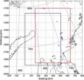
Fig. 3. The locations of the ice thickness charts for 4 March 2009 (blue rectangle) and 7 February 2009 (red rectangle) in the Kara Sea.

There are, to our knowledge, very few English-language studies on sea-ice thickness in the Kara Sea. The most comprehensive overview of ice conditions in the Kara Sea is given in Reference JohannessenJohannessen and others (2007). Their information on h _i is climatological in nature. Based on electromagnetic measurements in the southern Kara Sea, Reference Haas, Rupp, Uuskallio, Tuhkuri and KedsHaas and others (1999) reported typical H _i ranges of 1–1.5 m for pack-ice fields in April/May 1998. In our h _ch charts, typical values from early to mid-April ranged from 0.7 to 1.2 m in the same area. Throughout April 2009 the ice cover thickened according to the AARI ice charts. Winter 2008/09 was, however, much milder than winter 1997/98. In winter 1997/98 the Kara Sea was ice-covered at the end of November. In winter 2008/09 this happened in late January, i.e. almost 2 months later. Reference Divine, Korsnes, Makshtas, Godtliebsen and SvendsenDivine and others (2005) have studied fast-ice variability and its connection to atmospheric forcing in the northeastern Kara Sea.

First we examine ice conditions on 4 March 2009 where we have a coincident SAR/MODIS image pair and an AARI ice chart (Figs 4 and 5). The weather was cold: air temperature T _a was –27°C. In the AARI ice chart we see a narrow polynya near Novaya Zemlya, and that FYI thin ice (<70 cm) was the dominant ice type on the western side of the Yamal peninsula and north of it along the coast up to Severnaya Zemlya. The polynyas can be detected from the SAR image. In the MODIS chart, h _i ^M, the polynyas are only weakly visible, although the thin-ice areas (<30 cm) near the ice edge at the northern tip of Novaya Zemlya are identified well. We observe that the matrix W captured part of the FY thin-ice areas in addition to the very thin ice fields near the ice edge. There were errors in W in the fast-ice area located northeast of the Ob river estuary. In the overall thickness chart, h _ch, the major features are present concerning the spatial distribution of thin (h _ch < 70 cm) and thick ice (>70 cm) areas (Fig. 5).

Fig. 4. Datasets used in constructing the ice thickness chart on 4 March 2009. (a) The ice concentration (IC)-based weight matrix W; (b) the MODIS-based hi (dark blue shows no-data and cloudy areas; hi =1 m signifies hi > 1 m); and (c) the Envisat ASAR WSM image. All panels are shown in polar stereographic coordinates with reference longitude 63° E. Land area is marked dark brown in (a, b) and white in (c).

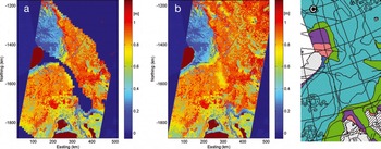
Fig. 5. The ice thickness charts on 4 March 2009. (a, b) The MODIS/SAR ice thickness chart (a) and the ASMR-E/MODIS/SAR thickness chart (b) (both charts in polar stereographic coordinates). The dark blue areas with h_i = –0.1 represent areas with no data, i.e. they are outside the SAR image or clouded regions (a). Land is marked dark brown. (c) The AARI ice chart on 4 March 2009, with color codes green = mainly thin FYI (30–70 cm), light blue = mainly medium FYI (70–120 cm), the rest being thin ice types (0–30 cm).

For comparison we also include the SAR/MODIS thickness chart which is the same chart as h _ch except that no thickness estimates are given to the cloud-covered region. We notice that the thin-ice area at the northern tip of Novaya Zemlya is retrieved well. We also observe that some thin-ice zones marked in the AARI chart and visible in the SAR image are detected in the northern part of h _ch which is masked off from the SAR/MODIS thickness chart.

The second h _ch chart shown here was constructed for 7 February 2009 (Figs 6 and 7). The AARI ice chart shows ice conditions 3 days earlier, on 4 February 2009. During the intervening 3 days the weather was cold. T _a stayed well below –30°C. According to the SAR imagery and the AARI ice chart, several very thin ice areas appeared in the northeastern part of the Kara Sea. These thin ice areas were detected well in the h _ch chart, where they were identified on the basis of MODIS chart h _i ^M. The western part of h _ch shows thinner ice than in the AARI chart. This was probably due to undetected warm ice fog in the MODIS ice surface temperature. The borderline in the north–south direction separating thicker (h _ch mostly >70 cm) and thinner ice areas refers to an artifact in the MODIS chart h _i ^M (Fig. 6b).

Fig. 6. (a) Envisat ASAR WSM image acquired on 7 February 2009. (b) MODIS/SAR ice thickness chart where the cloud-covered area is marked dark blue (h_i = –0.1). The value h_i = –0.1 is also used also to represent areas with no data. Both panels are shown in the same coordinate system as in Figure 4. Land (mostly islands) is marked white in (a) and dark brown in (b).

The ice thickness for the cloud-covered area in the h _ch chart (Fig. 7a) matched the AARI ice chart with the exception of the southeastern corner of the SAR image. Based on visual inspection of the SAR image, this area was covered by a mixture of open water and brash ice. In the h _ch chart it was estimated to have significantly thicker ice.

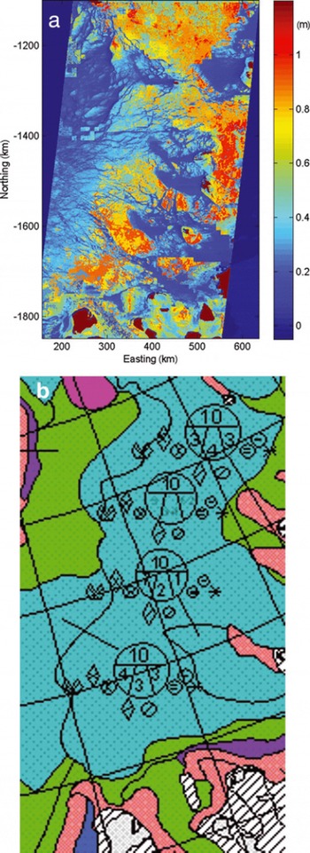
Fig. 7. (a) HIGHTSI/AMSR-E/MODIS/SAR ice thickness chart h_ch for 7 February 2009. (b) AARI ice chart on 4 February 2009, with color codes green = mainly thin FYI (30–70 cm), light blue = mainly medium FYI (70–120 cm), the rest being thin ice types (0–30 cm). The dark blue areas in (a) (h_i= –0.1) represent areas with no data. Land area is marked dark brown.

In our 32 MODIS/SAR image pair data, in >20% of the pairs the MODIS charts, h ^M _i, contained anomalies contradicting the information in the SAR imagery. If the h _ch charts are used more extensively, the resulting h _ch must be endowed with a quality flag indicating the reliability of the estimated h _i. The quality flag could be based on the human assessment of the result. It may be possible to automate the quality control process.

6. Accuracy Assessment of the Ice Thickness Chart

The accuracy of the h _ch charts was estimated by comparing them to the AARI ice charts. The absolute accuracy of the AARI ice charts using satellite data has not been established (personal communication from V. Smolyanitsky, 2013). To reduce the effect of ice drift we selected the h _ch charts that were computed within 1 day of the weekly AARI ice chart. This requirement was met seven times. Five h _ch charts used in the validation are for March (on 4, 10, 12, 18 and 25 March), one for December (25 December) and one for February (10 February).

From the AARI ice chart we can extract the three most dominant ice types and their relative concentrations for each polygon. For the seven selected AARI ice charts these ice types were typically nilas (h _i < 10 cm), young ice (h _i = 10–30cm), FYI thin ice (h _i =30–70cm) and FYI medium ice (h _i = 70–120 cm). In the accuracy analysis we simplified the situation slightly and used only three ice categories: very thin ice (h _i = 1–30 cm), FYI thin ice and FYI medium ice. Small open water areas were included in the thin ice category.

The validation of our h _ch charts is based on the relative frequencies of the three ice classes mentioned above. In the seven AARI ice charts, there are altogether 84 polygons which overlapped our h _ch charts. Each of these polygons has its own ice-class frequency distributions. Very small polygons (<20 km₂; 25% of all polygons) are studied separately.

We applied two different statistics to measure the closeness of the relative frequencies originating from the AARI ice charts and from our h _ch charts. The first statistic is the approximate mean ice thickness, h_x, of the polygon derived from the ice type frequencies:

(4)

where the subscript × refers to the dataset from which the class-wise frequencies freq _× originated, a for the AARI chart and e for h_ch. freq _× (c_k ) refers to the relative frequency of the ice type c_k in the polygon. We selected the midpoint of the thickness range of an ice type to represent its typical thickness.

For validation purposes we divided the polygons into ice categories according to the mean thickness h_a, i.e. if h_a was <30cm, it was labeled c ₁ä, etc. Using this criterion, the polygons belonged in 22 (26%) cases to the very thin ice category, in 41 (49%) cases to the FYI thin ice category and in 21 (25%) cases to the FYI medium ice category. In the same manner, we labeled the polygons based on h_e thickness. Because the thickness for each ice category was fixed, the label of a polygon depended only on the relative frequencies of the three ice types. This enables us to study the agreement of the frequency distributions on the basis of these two different polygon labelings. The comparison is presented in Table 2. Each row shows the number of polygons of same ice type category according to h_a (AARI charts). The columns shows the ice type categories for these polygons according to h_e. In the diagonal is the number of polygons where estimated and AARI-based ice thickness categories were in agreement. According to the error matrix shown in Table 2, the estimated ice type and the AARI-based ice type agreed in only 24% of cases for the very thin ice category. The results were better for the FYI thin ice category (agreement in 85% of cases) and the FYI medium ice category (agreement in 76% of cases).

Table 2. The error matrix obtained in the validation for 84 polygons (see Section 6). The table shows the comparison between the AARI ice chart based ice types (c_k ^a) vs ice thickness chart ice types (c_k ^e). The ice types are: very thin ice (c_1x ), FY thin ice (c_2x ) and FY medium ice c_3x . The subscript × indicates the data source, x=a for the AARI charts, x=e for the h _ch charts. The polygons were divided into ice categories according to the mean thicknesses h _a and h _e (see Eqn (4))

The second, and a more common, statistic to measure the closeness of two frequency distributions is a discrete variant of the Kolmogorov-Smirnov (KS) statistic (Reference Dudewicz and MishraDudewicz and Mishra, 1988). We calculate it as

(5)

where F _e and F _a denote the cumulative frequency functions of the h _ch chart and the AARI ice chart, respectively. The symbol c_k refers to the kth ice category.

The KS-statistic values for the polygons are shown in Figure 8. We chose the thresholds for the KS values subjectively. The chosen values were relatively large because there were only three classes, i.e. three jumps in the cumulative frequency function. We assessed that if the KS values stayed below 0.25, there was good consistency between F _e and F _a. Similarly we chose 0.4 to signify a threshold after which F _e and F _a resembled each other insignificantly.

Fig. 8. The Kolmogorov–Smirnov distance for the AARI ice chart polygons used in the h_ch validation. For every polygon the KS distance was calculated between the cumulative frequency functions extracted from the h_ch chart and the AARI ice chart, respectively. Very thin ice polygons (mean thickness <30 cm) and small polygons (area <20 km²) are marked green and and red. If the KS statistic lies below the green line, the class-wise frequency distributions of the the AARI chart and h_ch are considered consistent. If it is above the red line, the cumulative frequency distributions are inconsistent.

In 49% of cases, F _e was in good agreement with F _a. The agreement was poor or non-existent in 25% of cases. When studying the poor agreement polygons, we found that most of them were either small polygons (33% of poor agreement cases) or represented very thin ice (61% of poor agreement cases). Few poor agreement polygons were small and represented thin ice. The ice categories of the polygons were based on the h _a values as above. Of the small polygons, one-third stayed below the 0.25 threshold. The detection of very thin ice class was not successful. Only 19% of these polygons stayed below the 0.25 limit. The results for the polygons representing ice types FYI thin or FYI medium were good as long as these polygons were not small. Of these polygons, only in 10% of cases was the agreement deemed to be poor.

We must assess the validation results with caution, for several reasons. One reason is that the dataset does not cover the whole winter with regular intervals. Another reason is the limited number of suitable AARI ice charts. Five of the seven nearly coincident datasets were acquired in March. This probably led to a slight bias in the results. In the available sample set, 67% of polygons were correctly identified (Table 2). On the basis of the KS statistics, in 49% of cases the frequency distributions were consistent (Fig. 8). The results suggest that the accuracy of our ice thickness estimation method is good for the FYI thin and FYI medium ice categories.

A larger and temporally more evenly spread set of AARI ice charts also covering early winter would improve the accuracy assessment. We expect difficulties in the detection of thin-ice areas in the h _ch chart. The most effective way to detect these areas is to use the MODIS h _i ^M. If a thin-ice area is covered by clouds but is large enough, it can sometimes be identified relying on AMSR-E data (W matrix) or SAR data. However, our method often fails to detect thin-ice areas. On the basis of our limited validation data, we conclude that the proposed method gives realistic results in the thickness range 30–120 cm and is uncertain for very thin ice areas (<30cm).

During our validation process the inaccuracies in the AARI ice charts were not taken into account. As mentioned earlier, the level of accuracy is not quantitatively known. This is an additional caveat for the validation results. Validation data including field measurements are required for a truthful accuracy assessment. The best validation data would be a representative set of ice thickness measurements based on electromagnetic induction as in Reference Haas, Rupp, Uuskallio, Tuhkuri and KedsHaas and others (1999).

7. Conclusions

Currently no single satellite instrument is able to provide us with a near-real-time view of the spatial distribution of the ice mass with accurate ice thickness estimates, for both thin level ice and thick deformed ice. We have presented a method using multisensor satellite data and a HIGHTSI sea-ice thermodynamic model for estimation of the spatial distribution of the thin-ice fields (<1.2m in this dataset) present in the Arctic FYI zone.

We have utilized the strengths of each satellite sensor. The ice thickness up to 40cm is retrieved using MODIS ice surface temperature data and HIRLAM forcing data for cloud-free area. In cloud-covered regions, thin ice is located using the matrix Wderived from daily ice concentration changes, and a coarse ice thickness estimate is assigned. For thicker ice, thickness is retrieved from a combination of Envisat SAR image and modeled ice thickness background Hb, which consists of thermodynamically modeled H _i field modified by the matrix W. The accuracy of thin-ice detection is at its best if the thin-ice area is cloud-free. According to the validation exercise, the joint SAR σ ⁰ mapping together with Hb produced realistic results for the spatial distribution of FYI thin-ice (30–70cm) and medium ice (70–120 cm) types.

The obtained h _ch charts were validated against the frequency distributions of three sea-ice types which were extracted from seven weekly AARI ice charts. Altogether we had 84 ice chart polygons describing ice conditions.

According to the validation results for the h _ch charts, the FYI thin-ice and medium ice types were well identified. In this relatively small validation dataset, the accuracy in the ice thickness category classification varied around 80% depending on the applied accuracy criterion if the size of the polygon exceeded 20km². The detection of thin-ice polygons (<30 cm) succeeded only rarely, mainly because these polygons were typically very small. We also noted that about every fifth h _ch chart contained anomalies due to the MODIS-based h _i regions. We did not address the uncertainties present in our reference dataset. Hence our accuracy assessments are indicative in nature. For the total accuracy assessment, further validation work is needed.

Our method is not applicable for operative use due to the infrequency of the cloud-free MODIS data. In order to provide an operative method we have carried out experiments to locate thin-ice areas (thickness less than 30–40 cm) based on the AMSR-E data (Reference Von Lerber, Mäkynen, Similä, Sievinen and Hallikainenvon Lerber and others, 2012). We continue to test different approaches to utilize the AMSR-E data in thin-ice identification so that a h _ch chart could be computed daily. A campaign will be carried out where h _ch charts will be produced regularly during winter 2013/14 using AMSR data, and field observations will be collected. The current approach is, however, suitable to record the ice season evolution in the context of climate studies. We are studying how to incorporate ice drift (Reference KarvonenKarvonen, 2012) into our ice thickness estimation. One alternative is to utilize the modeled ice thickness fields of the mesoscale TOPAZ ocean/sea-ice model (Reference Bertino and LisæterBertino and Lisæter, 2008), which already contain sea-ice dynamics.