

1. Introduction
Many common human diseases and complex traits are highly heritable and are believed to be influenced by multiple genetic and environmental factors. A central goal of genetics, evolutionary biology and epidemiology is to identify genetic and environmental factors that influence complex traits and diseases, and to characterize the effects of these factors and their interactions (Lynch & Walsh, Reference Lynch and Walsh1998; Thomas, Reference Thomas2004). Genetic interactions (gene–gene and gene–environment interactions) have long been recognized as an important component of the genetic architecture of complex traits and diseases and are fundamentally important for understanding the genetics of complex traits and diseases (Mackay, Reference Mackay2001; Moore, Reference Moore2003; Flint & Mackay, Reference Flint and Mackay2009; Mackay et al., Reference Mackay, Stone and Ayroles2009).
There is a long history of the examination of genetic interactions in inbred plant and animal experimental crosses (Carlborg & Haley, Reference Carlborg and Haley2004) and human populations (Cordell, Reference Cordell2009; Thomas, Reference Thomas2010). Recent advances in genome-wide association studies (GWAS) have provided unparalleled opportunities for studying the genetic architecture of complex diseases (Hardy & Singleton, Reference Hardy and Singleton2009). In the past few years, these studies have identified many genetic variants associated with complex diseases (WTCCC, 2007; Hindorff et al., Reference Hindorff, Sethupathy, Junkins, Ramos, Mehta, Collins and Manolio2009). However, the main effects of the identified variants explain only a small proportion of the heritability of most complex diseases, motivating research interest in finding the remaining ‘missing’ heritability (Manolio et al., Reference Manolio, Collins, Cox, Goldstein, Hindorff, Hunter, McCarthy, Ramos, Cardon, Chakravarthi, Cho, Guttmacher, Kong, Kruglyak, Mardis, Rotimi, Slatkin, Valle, Whittemore, Boehnke, Clark, Eichler, Gibson, Haines, Mackay, McCarroll and Visscher2009). Since GWAS have not fully investigated interactions, it has been speculated that gene–gene and gene–environment interactions could be one of the potential sources of the missing heritability; this further boosts the investigation of genetic interactions (Cordell, Reference Cordell2009; Manolio et al., Reference Manolio, Collins, Cox, Goldstein, Hindorff, Hunter, McCarthy, Ramos, Cardon, Chakravarthi, Cho, Guttmacher, Kong, Kruglyak, Mardis, Rotimi, Slatkin, Valle, Whittemore, Boehnke, Clark, Eichler, Gibson, Haines, Mackay, McCarroll and Visscher2009; Cantor et al., Reference Cantor, Lange and Sinsheimer2010; Eichler et al., Reference Eichler, Flint, Gibson, Kong, Leal, Moore and Nadeau2010; Thomas, Reference Thomas2010).
Here, I review the statistical methods and related computer software that are currently being used for identifying genetic interactions for complex traits in animal and plant experimental crosses and human population-based association studies. The discussion covers the three broad issues in statistical analysis of genetic interactions, namely, the definition, the detection and the interpretation of genetic interactions. Significant advances in all the three related topics have been made in the past decades (Cordell, Reference Cordell2009; Thomas, Reference Thomas2010), and many of these are reviewed. All the methods discussed can be used in targeted genetic studies with moderate numbers of variants (for example, from hypothesis-driven candidate-genes or pathway-based studies), and some can be applied to large-scale genetic studies with large numbers of variants (for example, from GWAS).
One of the challenges in statistical analysis of genetic interactions is that genetic interaction is not uniquely defined. I first describe the general definition and meaning of interaction and then introduce the commonly used models that define an interaction term as a product of main-effect variables. I also discuss the issue that any statement about interaction is necessarily scale and model dependent, and outline the general principles for analysing interactions. The detection of genetic interactions involves two issues, modelling and computational methods, and can be viewed as a problem of high-dimensional data analysis. The development of statistical methods for high-dimensional data analysis has recently become one of the most important and active areas in statistics (Hesterberg et al., Reference Hesterberg, Choi, Meier and Fraley2008). Recently developed methods based on modern statistical techniques are mainly explored, including penalized likelihood approaches and hierarchical models, and the relationships among these methods are also discussed. The interpretation of genetic interactions has not been extensively discussed in the literature. The discussion is confined to key interpretations. Finally, I highlight some emerging directions and needs for making further progress.
2. Notation and challenges in analysing genetic interactions
We consider quantitative trait locus (QTL) mapping in experimental crosses from inbred animals or plants and population-based genetic association studies in humans. These two types of studies have the same observed data structure, and thus statistical methods can be fairly similar, while each has special problems. For each individual in the sample, observed data consist of a complex trait Y, a number of genetic markers G=(g 1, g 2, …, gm) and some environmental factors E=(z 1, z 2, …, zk), where m and k represent the numbers of makers and environmental factors, respectively. The trait phenotype Y can be continuous (e.g. body weight) or discrete (e.g. a binary disease indicator, counts). We consider experimental crosses (e.g. F2 intercross) or markers (e.g. single-nucleotide polymorphisms (SNPs)) that segregate three distinct genotypes. Therefore, each genotype variable gs is a three-level factor, indicating homozygous for the more common allele, heterozygous and homozygous for the minor allele, respectively. The genotyped markers can be densely distributed either across the entire genome or within some candidate genes, and for each case the number of markers can be large.
Our goal is to identify genomic loci that are associated with the complex trait, and to characterize their genetic effects. Since most complex traits and diseases are caused by interacting networks of multiple genetic and environmental factors, it is desirable to simultaneously consider multiple loci and environmental factors, and include gene–gene (epistatic) and gene–environment interactions in the model. Such joint analyses would improve the power for the detection of causal effects and hence lead to increased understanding about the genetic architecture of diseases. There are considerable challenges, however, to perform statistical analysis of genetic interactions:
• One has limited understanding of what the word ‘interaction’ means because it has no unique and explicit definition. Different definitions have different properties and lead to different statistical models and interpretations.
• With multiple genetic and environmental factors, there are many possible main effects and interactions, most of which are likely to be zero or at least negligible, leading to high-dimensional models and overfitting problems.
• There are many more potential interactions than main effects, which would require different modelling for main effects and interactions.
• Due to linkage disequilibrium, many genetic factors are highly correlated and nearly collinear, creating the difficulty of distinguishing disease-associated variants from others.
• Frequencies of multi-locus genotypes that define interactions can be very low, which creates variables with near-zero variance and thus requires special parameterization.
• The discreteness of genotype data can cause a separate identifiability problem, called separation, for discrete traits. Separation arises when a predictor or a linear combination of predictors is completely aligned with the outcome and can yield non-identified models (that is, have parameters that cannot be estimated).
These problems necessitate sophisticated techniques in all the steps of modelling, computation and interpretation for analysing genetic interactions. Some methods have been developed recently to overcome these problems and will be discussed in the following sections.
3. Definition of genetic interaction
The term ‘interaction’ generally refers to a phenomenon whereby two or more variables jointly affect the outcome response. In order to analyse and interpret interactions, it is important to understand how interactions are defined. In this section, I first discuss the general definition and meaning of statistical interactions, and then show how they can be made more concrete in the case of genetic analysis. We return to the issue of biological interpretation of statistical interaction later in the article.
(i) General definition of statistical interaction
As introduced earlier, the goal of QTL and association analysis is to investigate the relationship between the complex trait Y and the genetic and environmental factors, G=(g 1, g 2, …, gm) and E=(z 1, z 2, …, zk). For a normally distributed trait, this can be expressed as a statistical model
with the normal distribution assumption about the response variable Y, where E(·) is the expectation and η(·) represents a generally unknown function that relates the genetic and environmental factors to the expectation of Y.
With multiple genetic and environmental factors, even if we restrict our attention for simplicity to two-factor interactions, three different kinds have to be considered: (a) gene×gene (G×G), (b) gene×environment (G×E), (c) environment×environment (E×E). We do not discuss E×E interactions because they can be included in the model as covariates. While the formal definitions of G×G and G×E interactions are similar, their interpretations are rather different. I will briefly discuss their differences below.
With just two genetic factors g 1 and g 2, if the function of two factors η(g 1, g 2) can be replaced by the simpler form of two functions of one variable, i.e.
then there is no interaction between g 1 and g 2 (Cox, Reference Cox1984). This implies that the genotypic effect of locus g 1 (g 2) does not depend on the genotypes of g 2 (g 1). Therefore, these two genetic factors act in a way that appears causally independent. For G×E interactions, the condition of independence, η(g 1, z 1)=η1(g 1)+f 1(z 1), appears identical to the above-mentioned one, but the interpretation is quite different. Here, the concern is with regard to the stability of the genotypic effect of g 1 as the environmental condition z 1 varies. In genetic mapping, the environmental effect f 1(z 1) itself is of no direct interest, but can be an important component in controlling the potential confounding effect.
The converse conclusion that condition (2) is not satisfied is an indication of interaction between the two factors. In that case a change in the response due to a change in g 1 (g 2) does depend on the level of g 2 (g 1). However, any deviation from the independence condition (2) could be specified in various ways, leading to different types of interaction that may require different methods to identify. I here discuss the most commonly used method that considers the interaction as a product term of the main-effect variables. Because the genetic factors g 1 and g 2 are three-level factors, we naturally start with a two-way factorial model:
where i=1, 2, 3; j=1, 2, 3; g 1i represents the main effect of factor g 1 at level i; g 2j represents the main effect of factor g 2 at level j; and δij represents the interaction effect for factors g 1 and g 2 at levels i and j, respectively. With this model, the overall effect of factor g 1 at level i (i.e. genotypic effects) equals μ+g 1i+δij that does depend on the levels of g 2.
(ii) Cockerham model and alternatives
With no constraints on the parameters, model (3) is non-identifiable. In model (3), genotype factors g 1 and g 2 take on three values and therefore each has three main effects. However, the classical regression framework can estimate only two parameters – if all three were included, they would be collinear with the constant term and thus cannot be estimated uniquely (i.e. the model is non-identifiable).
One of the commonly used constraints on the parameters is to exclude the first level of each genotype factor from the model. The level that is excluded from the model is known as the reference or baseline condition. With this constraint, the number of main effects of each genotype factor and interactions between two factors reduces to two and four, respectively. Model (3) can be re-parameterized as
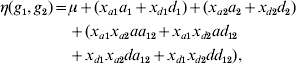
with xak=1 if gk=2, xak=0 otherwise, and xdk=1 if gk=3, xdk=0 otherwise, where ak and dk represent two main effects, and aa 12, ad 12, da 12 and dd 12 represent four interaction effects. In human genetic association studies, this model is called a co-dominant model (Thomas, Reference Thomas2004).
There are other options to construct constraints. The most widely used method is the Cockerham model (Cordell, Reference Cordell2002; Kao & Zeng, Reference Kao and Zeng2002; Zeng et al., Reference Zeng, Wang and Zou2005; Wang & Zeng, Reference Wang and Zeng2006, Reference Wang and Zeng2009; Cordell, Reference Cordell2009), which defines the main-effect variables as
For the Cockerham model, ak and dk correspond to the additive and dominance effects, respectively, and aa 12, ad 12, da 12 and dd 12 are interaction effects, called the additive×additive, additive×dominance, dominance×additive and dominance×dominance interactions, respectively. The Cockerham model can be easily understood by introducing the paternal and maternal indicators of the minor allele, ξp and ξm, centring by subtracting a conventional point 0·5. The indicator ξp (ξm) equals 1 if the paternal (maternal) allele is the minor allele and 0 otherwise. Therefore, the additive-effect variable can be expressed as xak=(ξp−0·5)+(ξm−0·5). This can be explained because a genotype consists of two alleles inherited from father and mother, respectively, and the paternal and maternal allelic effects are assumed to be identical. The dominance-effect variable can be expressed as xdk=−2(ξp−0·5)(ξm−0·5), representing the interaction between paternal and maternal alleles. The Cockerham model can be modified by centring the indicators ξp and ξm by subtracting their mean p (i.e. the allelic frequency) (Wang & Zeng, Reference Wang and Zeng2006, Reference Wang and Zeng2009). Therefore, we have xak=(ξp−p)+(ξm−p) and xdk=−2(ξp−p)(ξm−p).
The co-dominant and Cockerham models can be extended to include multiple genetic loci, environmental factors and their interactions:
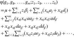
which consists of 2 m main effects and 2 m(m−1) two-way epistatic interactions. This model can be further extended to include higher-order interactions. We can see that even with a moderate number of factors m, the interaction model can include a huge number of parameters.
(iii) Generalized linear models
Generalized linear models have been widely used to analyse various types of non-normal complex traits (Yi & Banerjee, Reference Yi and Banerjee2009; Li et al., Reference Li, Reynolds, Pomp, Allison and Yi2010). A generalized linear model consists of three components: the linear predictor, the link function and the distribution of the outcome variable (McCullagh & Nelder, Reference McCullagh and Nelder1989; Gelman et al., Reference Gelman, Carlin, Stern and Rubin2003). The linear predictor is the same as that in the normal linear models described above. The link function h() is invertible and relates the mean of the outcome variable Y to the linear predictor:
or equivalently,
which obviously reduces to the normal linear model if h() is the identity function. The distribution of Y can take various forms, including normal, Gamma, binomial and Poisson distributions. Common forms of the link function for different assumed distributions of the outcome variable are h(η)=log (η) for Poisson treatment of counts, and logit=log (η/(1−η)), probit=Φ−1(η), or cloglog=log (−log(1−η)) for binary and binomial data. Therefore, generalized linear modelling provides a unified framework for statistical analysis; by choosing appropriate link functions and data distributions, some commonly used models, e.g. normal linear, logistic, probit and Poisson regressions, become special cases.
Interaction effects are more complicated in generalized linear models due to the link function between the linear predictor and the outcome variable:
• It is obvious from model (7) that the genetic effects correspond to a transformation of the mean of the outcome variable, h[E(Y)], rather than directly to the mean of the outcome variable E(Y) as in normal linear models. In a logistic regression, for example, genetic effects are defined on the scale of the log odds of a success outcome (i.e. Y=1), i.e. logit[Pr(Y=1)]=log[Pr(Y=1)/1−Pr(Y=1)].
• Some generalized linear models (for example, logistic and probit regressions) can be expressed as a normal linear model with an unobserved or latent outcome variable. For example, the logistic regression logit[Pr(Y=1)]=η(g 1,g 2, …,gm; z 1,z 2, …,zk) is equivalent to the latent normal linear model, u~N(η(g 1,g 2, …,gm; z 1,z 2, …,zk), 1.62), Y=1 if u>0 and Y=0 if u<0. Therefore, genetic effects in a logistic model actually correspond to the scale of a latent normally distributed outcome. The formulation of latent variables not only provides a computational trick but also a way to interpret the generalized linear models.
• Because genetic effects depend on the link function, it is possible that interaction effects on a link function may be removed by changing the link function. This is similar to the phenomenon for continuous responses that interaction on one scale may possibly be removed by a non-linear transformation of the scale (e.g. logarithmic and simple powers) (Cox, Reference Cox1984; Berrington & Cox, Reference Berrington and Cox2007). We may call an interaction removable if a transformation of the outcome scale can be found that induces additivity. I shall return to this issue later.
• Even with no multiplicative interaction terms in a generalized linear model, it is possible that the effects of a factor on the mean of the observed outcome E(Y) may depend on the levels of other factors in the model, because of the non-linear transformation h −1() (Gill, Reference Gill2001). Therefore, interaction effects are automatically introduced into all generalized linear models by a link function. However, these interactions do not affect the transformation of the observed data h[E(Y)]. Multiplicative interaction terms such as xa 1xa 2aa 11 are called the ‘variable-specific’ interaction terms, which are different from the ‘automatic’ interaction. If specifying these variable-specific terms in the model leads to improved fit, then we have successfully captured through parameterization at least some of the necessarily existent interaction between variables by the model specification.
(iv) Principles for analysing interactions
The widely used genetic interaction models define an interaction term as a product of main-effect variables, following the general definition of interaction (Cox, Reference Cox1984). For conventional models, guiding principles have been established for efficiently studying interactions. These principles could be more crucial for our problems because of the high-dimensional and correlated structure of genetic data. If appropriately applied, these principles can improve the analysis of genetic interactions (Kooperberg et al., Reference Kooperberg, Leblanc, Dai and Rajapakse2009).
1. The basic strategy for identifying interactions is to start from a simpler model involving only main effects, and then to introduce interaction effects when they improve the model fit to the data. The final interpretation of conclusions will be based on some simpler specification, for example, one involving some strong interaction terms (Cox, Reference Cox1984).
2. We prefer simultaneously fitting as many predictors as possible and introducing some hierarchical structure into the model (Gelman et al., Reference Gelman, Carlin, Stern and Rubin2003). This would allow us to take into account the correlation among the predictors. Applied to interaction analysis, therefore, it would be desirable to simultaneously include many correlated main effects and interactions.
3. Inputs with large main effects are more likely to have appreciable interactions with other inputs, although small main effects do not preclude the possibility of large interactions (Cox, Reference Cox1984; Gelman & Hill, Reference Gelman and Hill2007). Also, the interactions corresponding to larger main effects may be in some sense of more practical importance. This principle, sometimes referred to as ‘effect heredity’, has been used to build on interaction models (Hamada & Wu, Reference Hamada and Wu1992; Nelder, Reference Nelder1994; Chipman, Reference Chipman1996).
4. When an interaction of multiple factors is in the model, the lower-order variables comprising the interaction should also be present (Nelder, Reference Nelder1994). This is called the ‘effect hierarchy principle’. The reason for this is that if some contrast interacts with, say, z, and is therefore non-zero at some levels of z, it would normally be very artificial to suppose that the value averaged out exactly to zero over the levels of z involved in defining the ‘main effect’ for the contrast (Cox, Reference Cox1984). Applied to genetic interactions, genetic variants that have an interaction effect typically will also show some modest main effects (Kooperberg et al., Reference Kooperberg, Leblanc, Dai and Rajapakse2009). This could be used to explore interactions more efficiently.
4. Detection of genetic interaction
The detection of genetic interactions involves issues of statistical modelling and computing. A variety of methods for detecting gene–gene and gene–environment interactions have been proposed in the past decade (Musani et al., Reference Musani, Shriner, Liu, Feng, Coffey, Yi, Tiwari and Allison2007; Cordell, Reference Cordell2009; Kooperberg et al., Reference Kooperberg, Leblanc, Dai and Rajapakse2009; Thomas, Reference Thomas2010), and it is impossible to discuss all the available methods in this review. I focus on the most commonly used approaches: penalized likelihood regressions and hierarchical models. These two approaches are based on modern statistical techniques for high-dimensional data analysis and are powerful to handle the challenges in statistical analysis of genetic interactions, although alternative methods, including simple exhaustive searches (Marchini et al., Reference Marchini, Donnelly and Cardon2005), Bayesian partitioning algorithms (Zhang & Liu, Reference Zhang and Liu2007), non-parametric Bayesian methods (Zou et al., Reference Zou, Huang, Lee and Hoeschele2010) and various machine learning techniques (Ritchie et al., Reference Ritchie, Hahn, Roodi, Bailey, Dupont, Parl and Moore2001; Chen et al., Reference Chen, Liu, Zhang and Zhang2007; Lou et al., Reference Lou, Chen, Yan, Ma, Zhu, Elston and Li2007), have their own advantages.
(i) Penalized likelihood approach
In the classical framework, parameter estimation is obtained by maximizing the likelihood function. A linear model with either many coefficients or highly correlated variables can be non-identifiable. A standard approach to overcome the problem of non-identifiability is to add a penalty to the likelihood function, yielding the penalized likelihood function:
where β represents all effects and φ represents other parameters (e.g. residual variance). The logarithm of the likelihood function log f(y|β,φ) is a standard statistical summary of model fit; larger likelihood means better fit to data. For classical models, adding a parameter to a model is expected to improve the fit, even if the new parameter represents pure noise (Gelman & Hill, Reference Gelman and Hill2007). Therefore, the penalty term p(β) serves to control the complexity of the model and place some constraints or prior information on the parameters. Maximization of the penalized likelihood results in a penalized likelihood estimator.
The penalized likelihood function not only stabilizes parameter estimation but also provides criteria for model selection and comparison. The form of the penalty p(β) determines the general behaviour of the penalized likelihood approach. Small penalties would lead to large models with limited bias, but potentially high variance; larger penalties lead to the selection of models with fewer predictors, but with less variance. A traditional approach is to specify a penalty on the number of coefficients in the model, p(β)=λ |M|, where λ is a penalty parameter and |M| is the size of a model M. Many classical criteria have this form, including the Akaike information criterion (AIC) (λ=1) (Akaike, Reference Akaike1969) and the Bayesian information criterion (BIC) (λ=log(sample size)/2) (Schwartz, Reference Schwartz1978). These criteria have been widely used in earlier methods of multiple QTL mapping (Kao et al., Reference Kao, Zeng and Teasdale1999; Zeng et al., Reference Zeng, Kao and Basten1999). However, Broman & Speed (Reference Broman and Speed2002) showed that the original AIC and BIC tend to include many spurious QTLs and thus are not appropriate for model selection in QTL mapping, due to the large numbers of potential variables. Therefore, a variety of modifications to these classical criteria have been proposed, all seeking to control the false positive rate by using stronger penalty (Broman & Speed, Reference Broman and Speed2002; Bogdan et al., Reference Bogdan, Ghosh and Doerge2004; Baierl et al., Reference Baierl, Bogdan, Frommlet and Futschik2006).
For epistatic models, using a single penalty to control the overall complexity of the model would not be appropriate, because there are many more potential interactions than main effects. Therefore, two separate penalties should be used for main effects and pairwise epistatic interactions (Bogdan et al., Reference Bogdan, Ghosh and Doerge2004; Baierl et al., Reference Baierl, Bogdan, Frommlet and Futschik2006; Manichaikul et al., Reference Manichaikul, Moon, Sen, Yandell and Broman2009):
where λm and λi are the penalties on main effects and pairwise epistatic interactions, respectively, and |M|m and |M|i are the numbers of main effects and pairwise epistatic interactions. Bogdan et al. (Reference Bogdan, Ghosh and Doerge2004) and Baierl et al. (Reference Baierl, Bogdan, Frommlet and Futschik2006) suggested incorporating prior numbers of main effects and interactions to specify the penalty parameters λm and λi. Manichaikul et al. (Reference Manichaikul, Moon, Sen, Yandell and Broman2009) used the null distribution of the genomewide maximum LOD score to derive the penalty on main effects and the results of a two-dimensional, two-QTL scan to derive the penalty for the interaction terms. These methods employed forward and stepwise procedures to select main effects and interactions based on the corresponding penalized likelihoods. Manichaikul et al. (Reference Manichaikul, Moon, Sen, Yandell and Broman2009) further imposed an effect hierarchy principle, with the inclusion of a pairwise interaction requiring the inclusion of both corresponding main effects, and always included both additive and dominance terms for a QTL and all four epistatic effects for a pair of interacting QTLs. The method of Manichaikul et al. (Reference Manichaikul, Moon, Sen, Yandell and Broman2009) has been implemented in the freely available software R/qtl. R/qtl is an extensible, interactive environment for mapping QTLs in experimental populations derived from inbred lines (Broman et al., Reference Broman, Wu, Sen and Churchill2003).
The above penalty is called the L 0-penalty, which only involves the number of parameters and ignores the sizes of individual coefficients. Other penalty functions depend on the sizes of individual coefficients and can be more flexible. A popular method of this form uses an L 2-penalty (quadratic penalty) on all coefficients (excluding the intercept), corresponding to ridge regression (Hoerl & Kennard, Reference Hoerl and Kennard1970):
which is equivalent to maximizing the likelihood function subject to a size constraint on the sum of the squared coefficients, ![]() . The penalty parameter is predetermined usually by cross-validation.
. The penalty parameter is predetermined usually by cross-validation.
Ridge regression can handle the problem of collinearity and thus can simultaneously fit highly correlated variables. Malo et al. (Reference Malo, Libiger and Schork2008) applied ridge regression to fit all SNPs in a genomic region in genetic association studies and showed that such multiple-SNP analyses accommodate linkage disequilibrium among SNPs and have the potential to distinguish causative from non-causative variants. Park & Hastie (Reference Park and Hastie2008) proposed a logistic regression with L 2-penalty to fit genetic interactions in population-based case-control studies. They showed that the penalized logistic regression has a number of attractive properties for detecting genetic interactions. First, the L 2-penalty can deal with perfectly collinear variables (they sum to 1), and thus makes it possible to code each level of a factor by a dummy variable, yielding coefficients with direct interpretations (see eqn 3). As described earlier, this coding method cannot be applied to classical regression. Secondly, the L 2-penalty automatically assigns zero to the coefficients of zero columns and hence gracefully handles interaction models that consist of variables with near-zero variance. Thirdly, the quadratic penalty enables us to simultaneously fit a large number of factors and interactions in a stable fashion. Although the L 2-penalty has the above advantages, it cannot shrink any coefficients directly to zero and thus does not automatically remove variables from the model. Park & Hastie (Reference Park and Hastie2008) proposed a forward stepwise method based on the penalized likelihood to perform variable selection. Their algorithm obeys the effect hierarchy principle and also provides the option to accept an interaction even with no corresponding main effects in the model.
Another widely used penalized likelihood approach uses an L 1-penalty, leading to the lasso (least absolute shrinkage and selection operator) introduced by Tibshirani (Tibshirani, Reference Tibshirani1996). The lasso estimator is obtained by maximizing the likelihood function subject to a constraint on the sum of absolute values of the regression coefficients ![]() . This is equivalent to maximizing the following penalized likelihood function:
. This is equivalent to maximizing the following penalized likelihood function:
Compared to the ridge regression, a remarkable property of the lasso is that the L 1-penalty can shrink some coefficients exactly to zero and therefore automatically achieve variable selection. This can be intuitively explained by the fact that |βj| is much larger than |βj|2 for small βj and thus the constraint ![]() forces some βjs exactly to zero. Various optimization algorithms have been proposed to obtain the lasso estimator (Hesterberg et al., Reference Hesterberg, Choi, Meier and Fraley2008); Notably, the least angle regression (Efron et al., Reference Efron, Hastie, Johnstone and Tibshirani2004) and the co-ordinate descent algorithm (Wu & Lange, Reference Wu and Lange2008; Friedman et al., Reference Friedman, Hastie and Tibshirani2010) are the most computationally efficient.
forces some βjs exactly to zero. Various optimization algorithms have been proposed to obtain the lasso estimator (Hesterberg et al., Reference Hesterberg, Choi, Meier and Fraley2008); Notably, the least angle regression (Efron et al., Reference Efron, Hastie, Johnstone and Tibshirani2004) and the co-ordinate descent algorithm (Wu & Lange, Reference Wu and Lange2008; Friedman et al., Reference Friedman, Hastie and Tibshirani2010) are the most computationally efficient.
The feature of continuous shrinkage and variable selection along with the fast algorithms makes the lasso an effective method for genome-wide analysis of interacting genes. Tanck et al. (Reference Tanck, Jukema and Zwinderman2006) applied lasso penalized regression to detect epistatic interactions in association studies, with L 2-penalty on main effects and L 1-penalty on epistatic effects. Therefore, all main effects are always included in the model, while irrelevant interactions can be removed. Wu et al. (Reference Wu, Chen, Hastie, Sobel and Lange2009) developed a lasso penalized logistic regression for genome-wide association analysis in case-control studies. Their approach always selects a fixed number of predictors from all potential predictors. This yields a more efficient way of determining the penalty parameter. This novel strategy is similar to the composite model space approach that places an upper bound on the number of effects included in the model (Yi, Reference Yi2004; Yi et al., Reference Yi, Yandell, Churchill, Allison, Eisen and Pomp2005). For a given value of the penalty parameter, Wu et al. (Reference Wu, Chen, Hastie, Sobel and Lange2009) applied the co-ordinate descent algorithm to fit the lasso penalized logistic regression. Wu et al. (Reference Wu, Chen, Hastie, Sobel and Lange2009) handled interactions in two stages. In the first stage, the most important main effects of the predetermined number are identified; in the second stage, the two-way or higher-order interactions among the selected SNPs are examined. The method of Wu et al. (Reference Wu, Chen, Hastie, Sobel and Lange2009) has been implemented in the freely available software Mendel 9.0 at the UCLA Human Genetics web site.
(ii) Hierarchical models
Hierarchical modelling is an important tool in the analysis of complex and high-dimensional data and has been increasingly applied to QTL and association studies. Hierarchical models use a population distribution to structure some dependence into the parameters, thereby enabling to fit a large number of predictor variables. In contrast, non-hierarchical models generally cannot handle many variables simultaneously, because they are numerically unstable or tend to overfit data (i.e. fit the existing data well but lead to inferior prediction for new data). Hierarchical models are more easily interpreted and handled in the Bayesian framework. In Bayesian models, the population distribution of the parameters is often referred to as the prior distribution, and statistical inference is based on the posterior distribution that is proportional to the product of the likelihood function f(y|β,φ) and the prior distribution π(β,φ):
The posterior distribution contains all the current information about the parameters. Ideally one might fully explore the entire posterior distribution by sampling from the distribution p(β,φ|y) using Markov chain Monte Carlo (MCMC) algorithms (Gelman et al., Reference Gelman, Carlin, Stern and Rubin2003). For practical and computational purposes, however, it is desirable to have a fast algorithm that returns a point estimate of the parameters and standard errors. A commonly used point estimate is the posterior mode, that is, the single most likely value, which can be obtained by maximizing the posterior density p(β,φ|y), or equivalently its logarithm:
Compared with the penalized likelihood function (9), we can see that the posterior mode estimator is equivalent to the penalized estimator, with the logarithm of the prior density log π(β,φ) as the penalty. Therefore, with particular priors, hierarchical models can lead to the penalized likelihood approaches discussed above.
(a) Shrinkage priors
The prior distribution π(β,φ) plays an important role on the hierarchical modelling approach. A variety of priors have been proposed (Griffin & Brown, Reference Griffin and Brown2007), some of which have been adopted in QTL mapping and association analysis (Yi & Xu, Reference Yi and Xu2008; Yi & Banerjee, Reference Yi and Banerjee2009; Mutshinda & Sillanpää, Reference Mutshinda and Sillanpää2010; Sun et al., Reference Sun, Ibrahim and Zou2010). For models with a large number of potential variables, it is reasonable to assume that most of the variables have no or weak effects on the phenotype, whereas only a few have noticeable effects. Therefore, we can set up a prior distribution that gives each effect βj a high probability of being near zero. Such priors are often referred to as ‘shrinkage’ priors. In the following discussion, the prior distribution of φ is assumed to be non-informative and independent of β.
A class of shrinkage priors uses continuous distributions. A commonly used continuous shrinkage prior is the double exponential (also called Laplace) distribution (Tibshirani, Reference Tibshirani1996; Park & Casella, Reference Park and Casella2008; Yi & Xu, Reference Yi and Xu2008), ![]() , where λ is a shrinkage parameter and controls the amount of shrinkage; larger λ forces more coefficients near zero. With this prior, the log posterior density can be expressed as
, where λ is a shrinkage parameter and controls the amount of shrinkage; larger λ forces more coefficients near zero. With this prior, the log posterior density can be expressed as ![]() . Therefore, the posterior mode estimate of the coefficients β is the lasso penalized estimate (Park & Casella, Reference Park and Casella2008).
. Therefore, the posterior mode estimate of the coefficients β is the lasso penalized estimate (Park & Casella, Reference Park and Casella2008).
Another widely used continuous shrinkage distribution is the well-known Student's t-distribution, ![]() , where the hyperparameters μj, νj>0 and sj>0 are the location, the degrees of freedom and the scale parameters, respectively (Gelman et al., Reference Gelman, Carlin, Stern and Rubin2003). The location μj is usually set to zero. The hyperparameters νj and sj control the global amount of shrinkage in the effect estimates; larger νj and smaller s j2 induce stronger shrinkage and force more effects to be near zero. The family of the Student's t-distributions includes various distributions as special cases. At sj=∞, the t prior approaches a flat distribution, i.e. π(βj)∝1. Placing flat priors on all βj corresponds to a classical model, which usually fails in our problem as illustrated earlier. At νj=∞ and sj=s, the t prior is equivalent to a normal distribution βj~N(0,s 2), and thus the log posterior density can be expressed as
, where the hyperparameters μj, νj>0 and sj>0 are the location, the degrees of freedom and the scale parameters, respectively (Gelman et al., Reference Gelman, Carlin, Stern and Rubin2003). The location μj is usually set to zero. The hyperparameters νj and sj control the global amount of shrinkage in the effect estimates; larger νj and smaller s j2 induce stronger shrinkage and force more effects to be near zero. The family of the Student's t-distributions includes various distributions as special cases. At sj=∞, the t prior approaches a flat distribution, i.e. π(βj)∝1. Placing flat priors on all βj corresponds to a classical model, which usually fails in our problem as illustrated earlier. At νj=∞ and sj=s, the t prior is equivalent to a normal distribution βj~N(0,s 2), and thus the log posterior density can be expressed as ![]() . Therefore, the posterior mode estimate of the coefficients β is the ridge penalized estimate.
. Therefore, the posterior mode estimate of the coefficients β is the ridge penalized estimate.
Both the double exponential distribution and the Student's t-distribution can be presented as a two-level hierarchical model (Griffin & Brown, Reference Griffin and Brown2007; Yi & Xu, Reference Yi and Xu2008). The first level assumes that the coefficients βj's follow independent normal distributions with mean zero and unknown variances τj 2, and the second level assumes that the variances τj 2 follow some specified independent prior distributions:
where θj represent hyperparameters. The above two-level priors result in a scale mixture of normal distributions for the coefficients: ![]() . For the double exponential prior, π(τj 2|θj) is an exponential distribution Expon(λj 2/2) or equivalently a gamma distribution Gamma(1,λj2/2). For the Student-t prior, π(τj 2|θj) is a scaled inverse-χ2 distribution Inv-χ2(νj,sj 2) or equivalently an inverse gamma distribution Inv-gamma (
. For the double exponential prior, π(τj 2|θj) is an exponential distribution Expon(λj 2/2) or equivalently a gamma distribution Gamma(1,λj2/2). For the Student-t prior, π(τj 2|θj) is a scaled inverse-χ2 distribution Inv-χ2(νj,sj 2) or equivalently an inverse gamma distribution Inv-gamma (![]() ,
,![]() ).
).
The two-level hierarchical formulation has several advantages. First, it allows easy and efficient computation; conditional on the variances τj 2 the coefficients βj can be easily estimated and for some distributions π(τj 2|θj) (for example, the exponential and the inverse-χ2 distributions) the variances τj 2 also can be easily estimated. Secondly, it offers easy interpretation of the model; the coefficient-specific variances τj 2 result in different shrinkage amounts for different coefficients. Thirdly, it is flexible enough to encompass most versions of the penalized regression procedures and also lead to new hierarchical models by using new priors for the variances τj 2 or further modelling the hyperparameters θj (Griffin & Brown, Reference Griffin and Brown2007; Hoggart et al., Reference Hoggart, Whittaker, De Iorio and Balding2008; Kyung et al., Reference Kyung, Gill, Ghosh and Casella2010; Sun et al., Reference Sun, Ibrahim and Zou2010).
The second class of shrinkage priors assumes a discrete, two-component mixture distribution for each genetic effect, a normal distribution, and a point mass at zero (Yi et al., Reference Yi, Yandell, Churchill, Allison, Eisen and Pomp2005, Reference Yi, Shriner, Banerjee, Mehta, Pomp and Yandell2007b; Yi & Shriner, Reference Yi and Shriner2008):
where I 0 is a point mass at 0 and γj is a binary variable indicating the absence (γj=0) or presence (γj=1) of the effect βj. The variance τj 2 can be predetermined or treated as a random variable with an inverse-χ2 hyper-prior distribution: τj 2~Inv-χ2(νj,sj 2). The sparseness in the fitted model is controlled by the values of (νj,sj 2) and the prior inclusion probability p(γj=1) for each effect. The values of (νj,sj 2) can be chosen to control the prior expected mean and the prior confidence region of the proportion of the phenotypic variance explained by βj. Yi et al. (Reference Yi, Yandell, Churchill, Allison, Eisen and Pomp2005) proposed a method to choose the prior inclusion probabilities p(γj=1) for main effects and the G×G and G×E interactions (Yi et al., Reference Yi, Shriner, Banerjee, Mehta, Pomp and Yandell2007b; Yi & Shriner, Reference Yi and Shriner2008). These discrete ‘spike and slab’ priors lead to various Bayesian variable selection methods (Yi & Shriner, Reference Yi and Shriner2008).
(b) Estimating posterior modes
The continuous shrinkage priors result in continuous posterior distributions, allowing us to develop deterministic algorithms to quickly estimate the posterior mode. A variety of methods for computing the posterior mode have been developed for hierarchical models with continuous shrinkage priors, using the EM (expectation–maximization) algorithms by taking advantage of the two-level hierarchical formulation (Figueiredo, Reference Figueiredo2003; Gelman et al., Reference Gelman, Jakulin, Pittau and Su2008; Armagan & Zaretzki, Reference Armagan and Zaretzki2010) or other optimization algorithms (Genkin et al., Reference Genkin, Lewis and Madigan2007). These algorithms have been adapted to multiple QTL mapping and genetic association analysis (Zhang & Xu, Reference Zhang and Xu2005; Xu, Reference Xu2007, Reference Xu2010; Hoggart et al., Reference Hoggart, Whittaker, De Iorio and Balding2008; Yi & Banerjee, Reference Yi and Banerjee2009; Sun et al., Reference Sun, Ibrahim and Zou2010; Yi et al., Reference Yi, Kaklamani and Pasche2010). Among these developments, Yi & Banerjee (Reference Yi and Banerjee2009) and Yi et al. (Reference Yi, Kaklamani and Pasche2010) have attractive features and will be discussed below. The method of Yi & Banerjee (Reference Yi and Banerjee2009) has been implemented in the freely available software R/qtlbim (Yandell et al., Reference Yandell, Mehta, Banerjee, Shriner, Venkataraman, Moon, Neely, Wu, von Smith and Yi2007). R/qtlbim is an extensible, interactive environment for the Bayesian Interval Mapping of QTL, built on top of R/qtl (Broman et al., Reference Broman, Wu, Sen and Churchill2003), providing Bayesian analysis of multiple interacting QTL models for continuous, binary and ordinal traits in experimental crosses.
Yi & Banerjee (Reference Yi and Banerjee2009) and Yi et al. (Reference Yi, Kaklamani and Pasche2010) developed hierarchical generalized linear models with Student-t prior distributions on the coefficients for multiple interacting QTL mapping and genetic association studies. Yi & Banerjee (Reference Yi and Banerjee2009) discussed the choice of the shrinkage parameters νj and sj to favour sparseness in the fitted model. Yi et al. (Reference Yi, Kaklamani and Pasche2010) further proposed different scales sj for different types of effects (i.e. main effects, G×G and G×E interactions); this specification applies stronger shrinkage for interactions and thus allows more reliably a joint estimation of main effects and interactions. They used the EM algorithm to fit the model by estimating the marginal posterior modes of the coefficients βjs. The algorithm uses the two-level expression of the t prior distribution, treats the unknown variances τj 2 as missing data and replaces them by their conditional expectations at each E-step. The conditional expectations of τj 2 are independent of the response data, and thus the E-step is the same for different types of phenotypes. Given the variances τj 2, the prior distributions βj|τj 2~N(0,τj 2) can be included as additional ‘data points’ in the normal approximation of the generalized likelihood. Therefore, the coefficients βj can be estimated using the standard iterative weighted least squares (IWLS) for fitting classical generalized linear models. Yi & Banerjee (Reference Yi and Banerjee2009) incorporated the above EM algorithm into the standard package glm in R for fitting classical generalized linear models. This computational strategy takes advantage of the standard algorithm and software, and thus leads to a stable, flexible and easily used computational tool.
The above approach is built upon the generalized linear model framework, and therefore can deal with various types of continuous and discrete phenotypes and any models as implemented in the R package glm (e.g. normal linear, gamma, logistic, Poisson, etc.). This flexibility allows us to conveniently analyse data in different ways. As described earlier, interactions are defined relative to particular models and thus can be affected by a change in the model (Cordell, Reference Cordell2002; Berrington & Cox, Reference Berrington and Cox2007). The above approach would allow us to investigate whether an interaction can be removed by a transformation of the scale and to detect interactions that are only present in a particular model. The hierarchieal generalized linear models with Student-t priors on the coefficients includes various methods as special cases that have been designed to handle problems encountered in interacting QTL and association studies (Yi et al., Reference Yi, Kaklamani and Pasche2010). In addition, the above EM algorithm takes advantage of the two-level formulation of the t distribution and hence can be easily applied to other shrinkage priors (e.g. the double exponential distribution) with only modification on the conditional expectations of τj 2.
The hierarchical models can simultaneously analyse many covariates, main effects of numerous loci, epistatic and G×E interactions. For large-scale genetic data, however, we recommend performing a preliminary analysis to weed out unnecessary variables, or use a variable selection procedure to build a parsimonious model that only includes the most important predictors. The above algorithm can be incorporated into various variable selection procedures. Following the general principle for analysing interactions discussed earlier, Yi & Banerjee (Reference Yi and Banerjee2009) proposed a useful model search strategy, beginning with a model with no genetic effect but relevant covariates if any, and then gradually adding main effects and interactions into the model. This procedure differs from most variable selection methods by simultaneously adding or deleting many correlated variables.
(c) Sampling from the continuous posterior distribution
In Bayesian inference, it is more comprehensive to fully explore the posterior distribution than merely calculate the posterior mode. For the hierarchical models described above, this requires MCMC algorithms to generate samples from the posterior density. Various MCMC algorithms have been developed for hierarchical models with the continuous shrinkage priors discussed above (Bae & Mallick, Reference Bae and Mallick2004; Park & Hastie, Reference Park and Hastie2008; Hans, Reference Hans2009; Kyung et al., Reference Kyung, Gill, Ghosh and Casella2010), most taking advantage of the hierarchical formulation of the priors. These algorithms have recently been adapted to multiple QTL mapping and genetic association analysis (Xu, Reference Xu2003; Yi & Xu, Reference Yi and Xu2008; Sun et al., Reference Sun, Ibrahim and Zou2010), although they consider only main effects.
For hierarchical models with shrinkage priors that can be expressed as a mixture of normal distributions, it is easy to construct MCMC algorithms. Yi & Xu (Reference Yi and Xu2008) and Sun et al. (Reference Sun, Ibrahim and Zou2010) developed MCMC algorithms for mapping multiple QTLs using the hierarchical formulation of the double exponential and the Student-t priors. Since all priors for regression coefficients are conditionally Gaussian, a simple and unified scheme can be developed to update the coefficients βj regardless of the specific prior distributions on the variances τj 2. For the Student-t and double exponential priors, the conditional posterior distributions of the variances τj 2 have the standard form and thus can be easily sampled. Since the variances are separated from the data by the regression coefficients, the conditional distributions of the variances are independent of the response data. Therefore, the same updating scheme can be used to update the variances regardless of the response distribution. The advantage of MCMC samplers for hierarchical priors becomes more obvious when dealing with hyperparameters λ in the double-exponential prior and (ν, s) in the Student-t prior. The penalized likelihood approaches predetermine the penalty parameter using cross-validation, and the mode-finding algorithms usually preset the hyperparameters. In the fully Bayesian framework, however, the hyperparameters can be assigned appropriate hyperpriors and are updated along with other parameters (Park & Casella, Reference Park and Casella2008; Yi & Xu, Reference Yi and Xu2008; Kyung et al., Reference Kyung, Gill, Ghosh and Casella2010; Sun et al., Reference Sun, Ibrahim and Zou2010) or are estimated based on empirical Bayes using marginal maximum likelihood (Park & Casella, Reference Park and Casella2008; Yi & Xu, Reference Yi and Xu2008; Kyung et al., Reference Kyung, Gill, Ghosh and Casella2010; Sun et al., Reference Sun, Ibrahim and Zou2010); this procedure obviates the choice of the hyperparameters and automatically accounts for the uncertainty in its selection that affects the estimates of the regression coefficients.
The disadvantage of the above fully Bayesian approach is the intensive computation. This may restrict its application in genetic interaction analysis of large-scale data. However, these methods can provide richer information on the posterior of a regression coefficient and adequately reflect the uncertainty in estimating a parameter to be close to zero (Park & Casella, Reference Park and Casella2008; Kyung et al., Reference Kyung, Gill, Ghosh and Casella2010). The fully Bayesian analysis can return not only point estimates but also interval estimates of all parameters, and offers a natural means of assessing model uncertainty. As the mode-finding algorithms, the fully Bayesian methods can simultaneously fit many correlated variables and can distinguish important effects from a large number of correlated variables (Yi & Xu, Reference Yi and Xu2008; Sun et al., Reference Sun, Ibrahim and Zou2010).
(d) Bayesian variable selection using discrete priors
The hierarchical models with a discrete prior (16) are usually fitted using MCMC algorithms. A variety of algorithms have been proposed, some of which have been adapted to multiple interacting QTL mapping and genetic association analysis. Yi & Shriner (Reference Yi and Shriner2008) provide a comprehensive review on these methods. In this section, I describe the Bayesian multiple interacting QTL mapping methods that have been implemented in the freely available software R/qtlbim (Yi et al., Reference Yi, Yandell, Churchill, Allison, Eisen and Pomp2005; Yandell et al., Reference Yandell, Mehta, Banerjee, Shriner, Venkataraman, Moon, Neely, Wu, von Smith and Yi2007; Yi et al., Reference Yi, Banerjee, Pomp and Yandell2007a, Reference Yi, Shriner, Banerjee, Mehta, Pomp and Yandellb).
Yi et al. (Reference Yi, Yandell, Churchill, Allison, Eisen and Pomp2005) developed a Bayesian model selection method for mapping epistatic QTL in experimental crosses for complex traits, based on the discrete priors described above and the composite model space approach of Yi (Reference Yi2004). The key idea of this approach is to place an upper bound on the number of QTLs included in the model. Yi et al. (Reference Yi, Yandell, Churchill, Allison, Eisen and Pomp2005) set up the upper bound based on the Poisson prior on the number of QTLs with the prior mean determined by any initial analyses. Given the upper bound, Yi et al. (Reference Yi, Yandell, Churchill, Allison, Eisen and Pomp2005) used a vector γ of binary (0 or 1) variables indicating the absence or presence of the corresponding effects, equivalent to assuming the discrete prior (16). The vector γ determines the number of included QTLs and the activity of the associated genetic effects. The use of the upper bound and the indicator variables avoids the need to explicitly model the number of QTLs as in the previous Bayesian methods, allowing us to fit models of different dimensions, e.g. one versus two QTLs, without resorting to complicated reversible jump MCMC (Yi, Reference Yi2004). It also largely reduces the model space and provides an efficient way to walk through the space of models, spending more time at ‘good’ models.
Yi et al. (Reference Yi, Yandell, Churchill, Allison, Eisen and Pomp2005) developed an MCMC algorithm to generate samples from the posterior distribution and extended (2007b) the above method to include arbitrary environmental effects and G×E interactions, and to map interacting QTL for binary and ordinal traits based on the generalized probit models (2007a). The posterior samples can be used to summarize the genetic architecture and search for models with high posterior probabilities. Larger effects should appear more often, making them easier to identify. We use all the saved iterations of the Markov chain, corresponding to model averaging, which assesses characteristics of the genetic architecture by averaging over possible models weighted by their posterior probability. Various methods have been developed to graphically and numerically summarize and interpret the posterior samples (Yi et al., Reference Yi, Yandell, Churchill, Allison, Eisen and Pomp2005; Yandell et al., Reference Yandell, Mehta, Banerjee, Shriner, Venkataraman, Moon, Neely, Wu, von Smith and Yi2007).
5. Interpretation of genetic interaction
In QTL and genetic association analysis, there are many options available when modelling the data and computing the model. Once multiple QTLs are detected and a model with main effects and interactions are established, it is important to assess the fit of the model to the data and to our substantive (biological) knowledge, and to interpret the fitted models. Assessment and interpretation of interaction models have not been extensively discussed in the literature, possibly because identifying genetic interactions is a challenge and researchers are often so relieved to have detected interactions that there is a temptation to stop and rest rather than interpret the fitted model. Here, we discuss some methods for interpreting genetic interactions, including the issues of model checking, removable or non-removable interactions, average predictive genotypic effects and biological interactions.
(i) Model checking and assessment
A flexible method for model checking and assessment is posterior predictive checking that can be applied to complex genetic models and can assess the fit of the model to various aspects of the data. Posterior predictive checking proceeds by generating replicated data sets from the fitted model and then comparing these replicated data sets to the observed data set with respect to any features of interest. Assume that our data analysis has generated a set of simulations of the parameters, θ(s)=(β(s), φ(s)), s=1, …, n sim. For each of these draws, we simulate a replicated data set y rep(s) from the predictive distribution of the data, p(y rep|β(s), φ(s)). We check the model by means of discrepancy measures (test quantities) T(y, θ); several discrepancy measures can be chosen to reveal interesting features of the data or discrepancies between the model and the data. For each discrepancy variable, each simulated realized value T(y, θ(s)) is compared with the corresponding simulated replicated value T(y rep(s), θ(s)). Large and systematic differences between realized and replicated values indicate a misfit of the model to the data. In some cases, differences are apparent visually; otherwise, it can be useful to compute the p-value, p=Pr(T(y rep,θ)>T(y,θ)|y), to see whether the difference could plausibly have arisen by chance under the model. Although the posterior predictive model checking method is very flexible and quite simple, an important issue is how to choose the discrepancy quantities; this deserves future research.
A related approach to model checking is cross-validation, in which observed data are partitioned, with each part of the data compared with its predictions conditional on the model and the rest of the data. Cross-validation has been considered as a standard method for the expected predictive fit to new data. But it is computationally intensive and cannot be widely applied to Bayesian model assessment. For hierarchical models, however, the posterior predictive checking can produce results close to cross-validation if higher-level parameters are also simulated from the posterior (Green et al., Reference Green, Medley and Browne2009). Another approach is the deviance information criterion (DIC), which is a mixed analytical/computational approximation to an estimated predictive error (Spiegelhalter et al., Reference Spiegelhalter, Best, Carlin and van der Linde2002).
(ii) Removable or non-removable interactions
Statistical interactions are defined relative to particular models and thus can be affected by a change of modelling or outcome scale (Cordell, Reference Cordell2002; Berrington & Cox, Reference Berrington and Cox2007; Cordell, Reference Cordell2009; Thomas, Reference Thomas2010). We call an interaction ‘removable’ if a transformation of the outcome scale can be found to induce additivity (Berrington & Cox, Reference Berrington and Cox2007). Removable interactions are sometimes referred to as quantitative, whereas non-removable interactions are referred to as qualitative interactions. It may be important to investigate whether the detected interactions are removable or non-removable. If the interactions can be removed, the resulting interpretation may be improved and easily understood by a reasonable and interpretable model simplification.
For a continuous positive outcome, the Box-Cox technique (Box & Cox, Reference Box and Cox1964) can be used to find a non-linear transformation of the outcome that optimally fits the data (Cox, Reference Cox1984; Berrington & Cox, Reference Berrington and Cox2007). The Box-Cox transformations include commonly used logarithmic and simple powers as special cases. For binary data, the logistic or probit or complementary log scale may be effective (Berrington & Cox, Reference Berrington and Cox2007). The hierarchical generalized linear model approach of Yi & Banerjee (Reference Yi and Banerjee2009) and Yi et al. (Reference Yi, Kaklamani and Pasche2010) can deal with various types of continuous and discrete phenotypes and any generalized linear models, and allows us to conveniently analyse data using different models, providing a flexible way to investigate the nature of interactions.
(iii) Average predictive genotypic effects
Once we detect multiple QTLs with main effects and interactions, one of our interests is to infer which genotypes of these QTLs are associated with increased phenotypic value or disease risk, and to describe how a gene is associated with a trait or disease in combination with another gene or an environmental factor. This can be derived from the fitted models. However, challenges remain. First, single coefficients in an interaction model are less informative. In the presence of appreciable interaction, for example, main effects are rarely of direct concern because they represent effects among individuals with other variables equalling zero. Therefore, the genetic effects should always be interpreted jointly. Secondly, the predictors in genetic models are usually coded as functions of the genotypes, rather than the genotypes themselves, leading to further difficulty in interpreting the coefficients. Thirdly, for generalized linear models of interacting genes, the genetic effects are related to a non-linear transformation (i.e. the link function) of the observed data, and thus cannot be directly interpreted on the scale of the data.
One way to understand models with multiple interactions is to calculate the average predictive comparison of each of the inputs. The average predictive comparison is defined as the expected change in the outcome variable corresponding to a specified change in the input of interest averaging over some specified distribution of all other inputs and parameters (Gill, Reference Gill2001; Gelman & Hill, Reference Gelman and Hill2007). Yi et al. (Reference Yi, Kaklamani and Pasche2010) extend the average predictive comparison method to interpret genetic interaction models in case-control studies by presenting the average predictive probability of case for each of the SNPs and each pair of SNPs (or an SNP and a covariate) that significantly interact.
The method of Yi et al. (Reference Yi, Kaklamani and Pasche2010) can be extended to any genetic interaction model. Suppose that an interaction model has already been established. Generally, we define the marginal expectation E(y|gs=k) as the average predictive effect of the genotype gs=k of QTL s, and E(y|gs=k, gs ′=k′) as the average predictive effect of the two-locus genotype (gs, gs ′)= (k, k′) of QTL s and s′. For a binary trait, these expectations equal the average predictive probabilities as defined by Yi et al. (Reference Yi, Kaklamani and Pasche2010). These average predictive effects can be compared with each other, e.g. E(y|gs=k)−E(y|gs=k′), or with the overall mean E(y). Thus, the average predictive effects clearly show which genotypes of the detected QTL and their combinations are associated with increased or decreased phenotypic value or disease risk. Yi et al. (Reference Yi, Kaklamani and Pasche2010) developed a simple method to calculate the average predictive probability and graphically display the results. Their method can be extended to calculate the average predictive effects based on any generalized linear models.
(iv) Biological relevance of statistical interactions
The term ‘epistasis’ or ‘gene×gene interaction’ was originally used to describe instances in which the effect of a particular genetic variant was masked by a variant at another locus so that variation of phenotype with genotype at one locus was only apparent among those with certain genotypes at the second locus (Cordell, Reference Cordell2009; VanderWeele, Reference VanderWeele2010). This original concept of epistasis is different from the definitions of statistical interactions that are usually used in statistical analysis of complex traits. Phillips (Reference Phillips2008) recently discussed the ambiguity in the term ‘epistasis’ and defines three distinct forms of epistasis: statistical epistasis, compositional epistasis and functional epistasis. Phillips (Reference Phillips2008) defined ‘statistical epistasis’ as a departure from marginal effects in a statistical model, much closer to the statistical interaction described earlier. The term ‘compositional epistasis’ refers to epistasis in Bateson's original sense of the term, while the term ‘functional epistasis’ describes the physical molecular interactions between various proteins (and other genetic elements) (Phillips, Reference Phillips2008). Compositional epistasis is a more biological form of interaction than the commonly used statistical epistasis, but does not necessarily imply functional epistasis. These distinct concepts of epistasis can be also applied to gene–environment interactions (Thomas, Reference Thomas2010; VanderWeele, Reference VanderWeele2010).
Most statistical methods for analysing genetic interactions actually test statistical interactions. However, the extent to which statistical interaction implies biological or functional interaction has been extensively debated in both the genetics and epidemiological literature. A prevailing opinion is that statistical tests for interactions are of limited use for elucidating epistasis in the biological sense of the term (Cordell, Reference Cordell2009). However, VanderWeele recently showed some relationship between statistical interaction and compositional epistasis, and derived conditions under which statistical interactions correspond to compositional epistasis (VanderWeele, Reference VanderWeele2010; Vanderweele & Laird, Reference Vanderweele and Laird2010). These empirical conditions are quite strong, but the procedures proposed may provide a useful strategy to study biological interactions.
6. Needs for further progress
(i) Gene or pathway level information
Candidate gene studies usually consist of data at different levels, i.e. genetic variants (e.g. haplotype-tagging SNPs) within multiple candidate genes which may be functionally related or from different pathways. Most of the statistical methods that are recently being used consider only individual-level predictors (i.e. SNPs and covariates) and ignore the hierarchical structure of the data and gene or pathway-level information. It is biologically expected that genetic variants within a gene would influence the phenotype more similarly than those in different genes (Hung et al., Reference Hung, Brennan, Malaveille, Porru, Donato, Boffetta and Witte2004). Often, rich gene or pathway-level information is available (Rebbeck et al., Reference Rebbeck, Spitz and Wu2004), including simple pathway indicator variables, genomic annotation or pathway ontologies, functional assays, in silico predictions of function or evolutionary conservation or simulation of pathway kinetics (Thomas et al., Reference Thomas, Conti, Baurley, Nijhout, Reed and Ulrich2009). Therefore, there is a growing need to develop sophisticated approaches that model the multilevel variation simultaneously and incorporate gene or pathway-level data into the model (Dunson et al., Reference Dunson, Herring and Engle2008; Thomas, Reference Thomas2010).
Hierarchical models provide a natural and efficient way of incorporating the external information about candidate genes into the analysis. One way of including the gene-level information in the hierarchical models is to model the prior means in the prior distributions of coefficients βj using gene-level predictors. This approach allows us to pool the information in the same genes and thus would provide more effective inference about the genetic effects. Recent developments of penalized regressions for high-dimensional data may provide alternative improved ways to deal with specific structures in candidate genes. It is well known that the original lasso regression does not effectively account for the relationship among a group of correlated predictors and tends to select individual variables from the grouped variables. The elastic net (Zou & Hastie, Reference Zou and Hastie2005) is a generalization of the lasso regression, which introduces an additional penalty or prior to incorporate the correlation of predictors into the model (Kyung et al., Reference Kyung, Gill, Ghosh and Casella2010). The elastic net can be implemented in a hierarchical fashion combining variable selection at lower levels (e.g. among SNPs within a pathway) and shrinkage at higher levels (e.g. between genes within a pathway or between pathways).
(ii) Modelling genetic interactions hierarchically
The effect heredity and hierarchy are two important principles for the statistical analysis of interaction (Chipman, Reference Chipman1996; Hamada & Wu, Reference Hamada and Wu1992; Nelder, Reference Nelder1994). These principles pose certain dependence of interactions on their main effects. Since with many predictors there are a huge number of potential interactions, a simple inclusion of interactions can degrade the model fit and thus preclude effective estimation of main effects and interactions. Although these two principles have been noticed in some of the previous methods of genetic interactions, there is a clear need for further studies in the future. Recently, the lasso penalized regression has been extended to incorporate the effect heredity and hierarchy principles (Yuan et al., Reference Yuan, Joseph and Lin2007; Zhao et al., Reference Zhao, Rocha and Yu2009; Choi et al., Reference Choi, Li and Zhu2010). Theoretical and empirical results have showed that these extensions outperform the previous methods for detecting interactions. These new developments should be adapted to the statistical analysis of genetic interactions. Another promising approach could be modelling interactions in a structured way, for example, with larger variances for interactions whose main effects are large. This type of priors can incorporate the effect heredity principle in a more continuous form.
(iii) Next-generation sequencing and rare variants in genetic interactions
The genetic aetiology of common (or complex) human diseases is determined by both common and rare genetic variants (Bodmer & Bonilla, Reference Bodmer and Bonilla2008; Schork et al., Reference Schork, Murray, Frazer and Topol2009). Since GWAS have so far focused on common variants (with minor allele frequency (MAF)≳5%) in the human genome, it has been speculated that rare variants might account for at least some of the heritability that GWAS have missed (Manolio et al., Reference Manolio, Collins, Cox, Goldstein, Hindorff, Hunter, McCarthy, Ramos, Cardon, Chakravarthi, Cho, Guttmacher, Kong, Kruglyak, Mardis, Rotimi, Slatkin, Valle, Whittemore, Boehnke, Clark, Eichler, Gibson, Haines, Mackay, McCarroll and Visscher2009; Cirulli & Goldstein, Reference Cirulli and Goldstein2010; Eichler et al., Reference Eichler, Flint, Gibson, Kong, Leal, Moore and Nadeau2010). Several studies have already shown that rare variants play an important role in genetic determination for some diseases (Cohen et al., Reference Cohen, Kiss, Pertsemlidis, Marcel, McPherson and Hobbs2004, Reference Cohen, Boerwinkle, Mosley and Hobbs2006; Ahituv et al., Reference Ahituv, Kavaslar, Schackwitz, Ustaszewska, Martin, Hebert, Doelle, Ersoy, Kryukov, Schmidt, Yosef, Ruppin, Sharan, Vaisse, Sunyaev, Dent, Cohen, McPherson and Pennacchio2007; Romeo et al., Reference Romeo, Pennacchio, Fu, Boerwinkle, Tybjaerg-Hansen, Hobbs and Cohen2007, Reference Romeo, Yin, Kozlitina, Pennacchio, Boerwinkle, Hobbs and Cohen2009; Azzopardi et al., Reference Azzopardi, Dallosso, Eliason, Hendrickson, Jones and Rawstorne2008; Ji et al., Reference Ji, Foo, O'Roak, Zhao, Larson, Simon, Newton-Cheh, State, Levy and Lifton2008; Nejentsev et al., Reference Nejentsev, Walker, Riches, Egholm and Todd2009). Recent advances in next-generation sequencing technologies facilitate the detection of rare variants, making it possible to uncover the roles of rare variants in complex diseases.
As a single rare variant contains little variation owing to low MAF (<0·5 or 1%), statistical methods that test variants individually provide insufficient power to detect causal rare variants. Therefore, association analysis of rare variants requires sophisticated methods that can effectively combine the information across variants and test for their overall effect (Manolio et al., Reference Manolio, Collins, Cox, Goldstein, Hindorff, Hunter, McCarthy, Ramos, Cardon, Chakravarthi, Cho, Guttmacher, Kong, Kruglyak, Mardis, Rotimi, Slatkin, Valle, Whittemore, Boehnke, Clark, Eichler, Gibson, Haines, Mackay, McCarroll and Visscher2009). Several approaches have been developed to analyse rare variants, including the Collapsing, Simple-Sum and Weighted-Sum methods (Li & Leal, Reference Li and Leal2008; Madsen & Browning, Reference Madsen and Browning2009; Morris & Zeggini, Reference Morris and Zeggini2010; Price et al., Reference Price, Kryukov, de Bakker, Purcell, Staples, Wei and Sunyaev2010). These methods summarize multiple rare variants by weighting them equally (Li & Leal, Reference Li and Leal2008; Morris & Zeggini, Reference Morris and Zeggini2010) or on the basis of estimated standard deviation (Madsen & Browning, Reference Madsen and Browning2009) or functional prediction (Price et al., Reference Price, Kryukov, de Bakker, Purcell, Staples, Wei and Sunyaev2010). Recently, penalized likelihood approach and hierarchical models have been applied to rare variants analysis (Zhou et al., Reference Zhou, Sehl, Sinsheimer and Lange2010; Yi & Zhi, Reference Yi and Zhi2010). These methods have focused on rare variants in a gene or region, and exclude genetic interactions in the analysis. Since complex diseases are usually influenced by multiple genes and environmental factors and their interactions, it would be important to develop sophisticated methods for jointly analysing all rare variants in multiple genes and gene–environment and gene–gene interactions.
(iv) Using interaction models for risk prediction
GWAS have raised expectations for predicting individual susceptibility to common diseases using genetic variants (Wray et al., Reference Wray, Goddard and Visscher2008; Kraft et al., Reference Kraft, Wacholder, Cornelis, Hu, Hayes, Thomas, Hoover, Hunter and Chanock2009). Previous methods using only a limited number of significant variants have typically failed to achieve satisfactory prediction performance (Jakobsdottir et al., Reference Jakobsdottir, Gorin, Conley, Ferrell and Weeks2009; Kraft & Hunter, Reference Kraft and Hunter2009). Recent studies show that joint analysis of a large number of genetic variants can improve the risk prediction performance (Meuwissen et al., Reference Meuwissen, Hayes and Goddard2001; Lee et al., Reference Lee, van der Werf, Hayes, Goddard and Visscher2008; de los Campos et al., Reference de los Campos, Naya, Gianola, Crossa, Legarra, Manfredi, Weigel and Cotes2009; Wei et al., Reference Wei, Wang, Qu, Zhang, Bradfield, Kim, Frackleton, Hou, Glessner, Chiavacci, Stanley, Monos, Grant, Polychronakos and Hakonarson2009; Hayashi & Iwata, Reference Hayashi and Iwata2010; Yang et al., Reference Yang, Benyamin, McEvoy, Gordon, Henders, Nyholt, Madden, Heath, Martin, Montgomery, Goddard and Visscher2010). However, the previous studies have not included interactions into the predictive models. If G×G and G×E interactions are present, adding these interactions to a predictive model should increase the accuracy of prediction. Therefore, jointly modelling genetic, environmental factors and their interactions has important implications for disease risk prediction and personalized medicine (Clark, Reference Clark and Clegg2000; Moore & Williams, Reference Moore and Williams2009). Because frequencies of multi-locus genotypes that define interactions are usually low, inclusion of interactions may not largely improve the overall prediction in the entire population based on the commonly used receiver operating characteristic (ROC) curve (Bjørnvold et al., Reference Bjørnvold, Undlien, Joner, Dahl-Jørgensen, Njølstad, Akselsen, Gervin, Rønningen and Stene2008; Clayton, Reference Clayton2009). However, the interaction models can identify combinations of multiple susceptibility loci that confer very high or low risk, and hence can be highly predictive for subsets that carry certain combinations of interacting variants (Yi et al., Reference Yi, Kaklamani and Pasche2010). Unfortunately, most of the genetic association studies have so far not addressed G×G and G×E interactions, and thus the translation of scientific understanding about G×G and G×E interactions into risk assessment and genomic profiling has been limited.
7. Conclusions
Genetic interactions are worth studying for many reasons (Cordell, Reference Cordell2009; Thomas, Reference Thomas2010). First, modelling G×G and G×E interactions can increase the power to detect additional variants or genes and more accurately characterize the genetic effects, Secondly, detection and characterization of genetic interactions will help elucidate the biological and biochemical pathways that underpin disease. Finally, including significant interactions in risk prediction models can have important implications for disease risk prediction and personalized medicine. Recent advances in GWAS have provided unparalleled opportunities for investigating the genetic architecture of complex diseases. However, most of these studies have used a single-locus analysis strategy and thus ignored interactions. Therefore, the follow-up studies should focus on investigating genetic interactions and other complexities (Manolio et al., Reference Manolio, Collins, Cox, Goldstein, Hindorff, Hunter, McCarthy, Ramos, Cardon, Chakravarthi, Cho, Guttmacher, Kong, Kruglyak, Mardis, Rotimi, Slatkin, Valle, Whittemore, Boehnke, Clark, Eichler, Gibson, Haines, Mackay, McCarroll and Visscher2009; Cantor et al., Reference Cantor, Lange and Sinsheimer2010). However, this requires sophisticated statistical methods. As discussed in this article, there are a variety of approaches that can be used to analyse genetic interactions. The integration of the modern high-dimensional statistical methods and the specific form of genetic data and external biological knowledge will further improve the power to detect complex interactions.
This work was supported in part by the following research grants: NIH 2R01GM069430-06, NIH R01 GM077490 and NIH R01 CA112520-06A2.
