Introduction

Earlier studies of the areal distribution of ¹⁸O/¹⁶O values relative to standard mean ocean water (SMOW) (δ¹⁸O, in ‰) in northeastern Canada and northwest Greenland (e.g. Reference KoernerKoerner, 1979) have focused on bivariate relationships between δ¹⁸O and independent variables such as mean annual surface temperature, surface elevation, and distance to the coastline. In this study we assess the areal distribution of δ¹⁸O and covariation of the independent variables using stepwise regression analysis.

Our compilation of δ¹⁸O values determined from firn samples collected in ice caps and snow fields in northeastern Canada lists 23 sites (Fig. 1 and Table 1; site 1 on the Norih Ice Cap, Greenland, is included because it shares the same lower troposphere flow with at least nine other sites to the west). Data for one other site on the Devon Icc Cap (at about 115 km on the traverse route, 75.60° N, 83.3° W, 500 m (Reference Koerner and RussellKoerner and Russell, 1979), and from two other ice caps (Meighen Ice Cap, 79.95° N, 99.4° W, 270 m (Reference Koerner and PatersonKoerner and Paterson, 1974); Barnes Ice Cap (five sites centered at about 69.75° N, 72.0° W at elevations between 500 and 870 m (Reference Hooke and ClausenHooke and Clausen, 1982) were excluded from the compilation because the samples were collected from areas either of net ablation, or of intense summer melt and percolation. On some of the ice caps, ice shelves, and snow fields lisied in Table 1 there are many more sites for which δ¹⁸O values have been determined. We selected relatively few sites from each in an attempt to attain a regionally representative (unbiased) database.

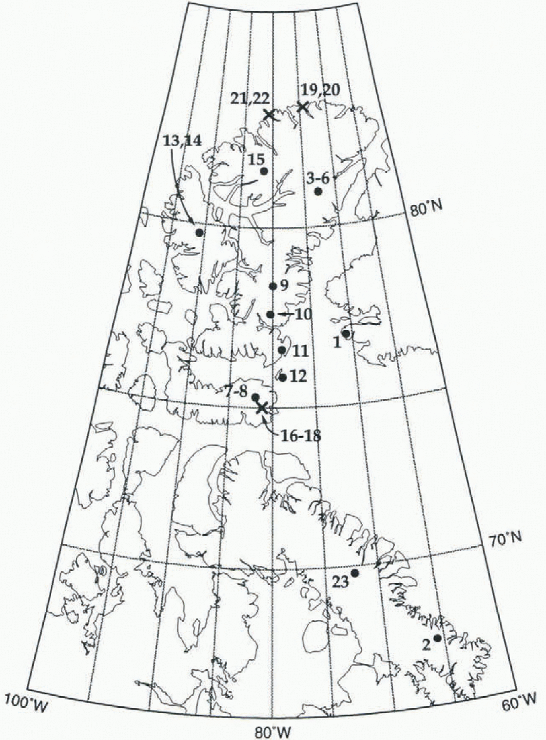
Fig. 1. Location of sites listed in Table 1. Full circles indicate sites for which mean annual sulfate temperature could be determined from surface data (T_s). Crosses indicate sites for which mean annual surface temperature was determined exclusively from remotely sensed data (T_r).

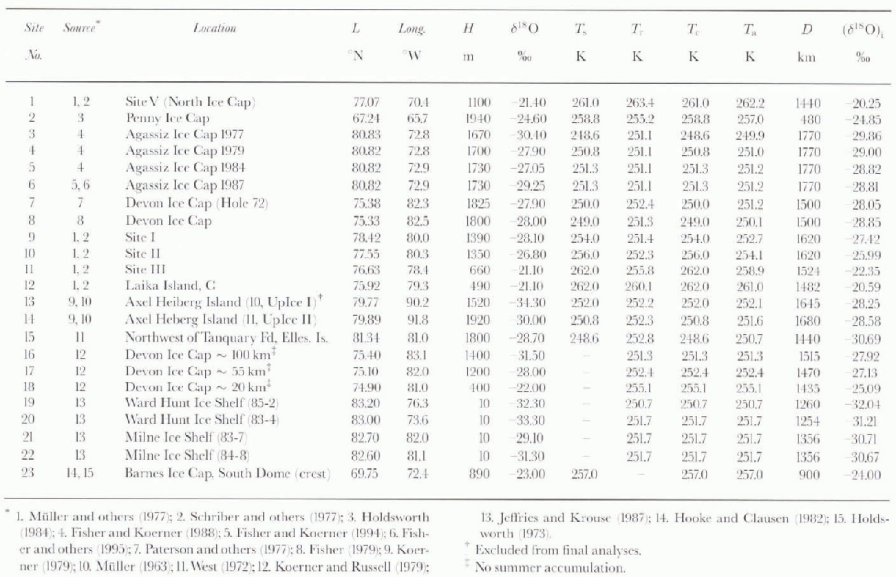
Table 1. Database summary and modeled results

Database

Data on latitude (L) in degrees north and longitude, surface elevation (H) in m, and mean annual surface temperature (T_s, in K) normally determined from firn temperature measurements at a depth of 10 m, were staled in the original reports for approximately half of the sites. Missing data were obtained as follows:

• (1) L as well as longiiude values by interpolation after plotting traverse routes from starting points and marking stated distances along routes.

• (2) H values by interpolation from the latest topographic maps available, in some cases show in the original reports.

• (3) T_s values, by extrapolation of shallow firn-temperature measurements at the site (e.g. inferring 10m temperature from a temperature observation at a depth of 4 m in summer), or by interpolation of deep firn-temperature measurements at nearby sites, or by interpolation from isotherm patterns or meteorological station data as compiled in standard reference publications (e.g. Reference Vowinckel, Orvig and OrvigVowinkel and Orvig, 1970).

The methods described above to obtain T _s for sites where temperature data were not reported, could not be applied in the case of seven locations (sites 16–22). To include these in the study, we obtained remotely sensed mean annual surface temperature values (T _r) in K by bilinear interpolation from Nimbus-7 Temperature Humidity Infrared Radiometer (THIR) data for 1979 (Reference ComisoComiso, 1994).

The T _s value entered for a location at the crest on the South Dome of the Barnes Ice Cap (site 23) presented a special case. A firn-temperature measurement at a depth of 20m (−8°C) was considered to be higher than the actual mean annual surface temperature due to melting, percolation, and freezing processes, and in a preceding study the surface temperature was estimated at −15°C (Reference HoldsworthHoldsworth, 1973). This estimate was based on meteorological observations at Dewar Lakes (68.65° N, 74.2° W, 518 m) using a lapse rate of 6.5° C km⁻¹ in the extrapolation. We included this site after a first run of the analyses were completed (personal communication from R. LeB. Hooke, August 1996) and did not obtain T _r data for it. Nevertheless, based on L. T _s, and T _r data from the Penny and Devon Ice Caps (sites 2 and 7) and using lapse rates derived from standard atmospheres for 60° N and 75° N (Reference Cole, Court, Kantor and ValleyCole and others, 1965) in the interpolation, the mean surface temperalure for site 23 was estimated at −17°C. Therefore we entered an intermediate T _s value of 257 K in the database.

Values of mean annual shortest distance to the open ocean (D) in km were measured between a site location and the position of the 10% sea-ice-concentration boundary determined from Nimbus-7 Scanning Multi-channel Microwaxe Radionieler (SMMR) data for 1978–87 (Reference Gloersen, Campbell, Cavalieri, Comiso, Parkinson and ZwallyGloersen and others, 1992). No attempt was made to measure distance to regional polynya during periods of precipitation (e.g. Schriber and others, 1977).

The database thus assembled has inherent shortcomings concerning the two principal variables, δ¹⁸O and T_s T_r:

• (1) The compiled δ¹⁸O values are representative of a wide variety of depositional environments (e.g. Reference Fisher, Koerner, Patrrson, Dansgaard, Gundestrup and RechFisher and others, 1983) as well as accumulation periods, many not overlapping and ranging from fall through spring snow samples to an undetermined number of summer and winter firn layers.

• (2) Approximately half of the compiled T_s values were obtained indirectly, as described above, or indirectly by extrapolation or interpolation.

• (3) Bilinear interpolation of THIR data does not necessarily produce a more reliable temperature value for a specific site due to the topographic complexity of the region, particularly when the data resolution (about 30 × 30 km (Reference ComisoComiso, 1994)) in seven of the sites includes both land areas (snow, firn, ice and exposed rock surfaces) and sea areas (snow on sea ice, sea ice and water surfaces).

The undesirable attributes of the δ¹⁸O and T _s, T _r data mentioned above, as well as the relatively small sample available for this study (varying between N14 and N23; N denotes the number of sites in a set), require that a cautionary note be applied to our findings. The shortcomings presented by the small sample are addressed, in part, using the adjusted coefficient of determination statistic, R_a ² (correlation coefficient, R, squared and modified for sample size (e.g. Reference Tabachnick and FidellTabachnick and Fidell, 1989)). In the following sections, the statistics are significant at the 99.99% confidence level (F statistic under the null hypothesis showing a probability of P≤0.0001) unless stated Otherwise. A confidence level selected for a particular model to determine which variables contribute at that level (or better) to the explanation of variation, is a separate statistic from the P-value attained by the model (e.g. Reference Davis and SampsonDavis and Sampson, 1973).

Preliminary Analyses

Stepwise regression analysis of the data for 16 sites and of the form δ¹⁸O = f(L, H, T_s, D) at the 90% confidence level showed that only T _s entered the model in the forward mode, or remained in the model in the backward mode (in the case of small datasets it is advisable to run stepwise analyses both forward and backward as the results may be different (e.g. Davisand Sampson, 1973)). Nevertheless, bivariate statistics for δ¹⁸O = f(T _c) showed a moderate correlation (Table 2) N16; R is 0,840, R_a ² is 0.684, root mean square residual (rms) is 2.09) (henceforce all bivariate regression analyses are summarized in Table 2 for easy comparison), In Figure 2 the data for site 13 showed the largest departure from the fitted line (≤3 rms). Its exclusion, to be fully justified, would require a departure ≫3 rms: however, in a small sample and everything else being equal, data for a single site may greatly modify final results. Therefore, we excluded data from that site (N15; R is 0.931, R_a ² is 0.856, rms is 1.24):

(1)

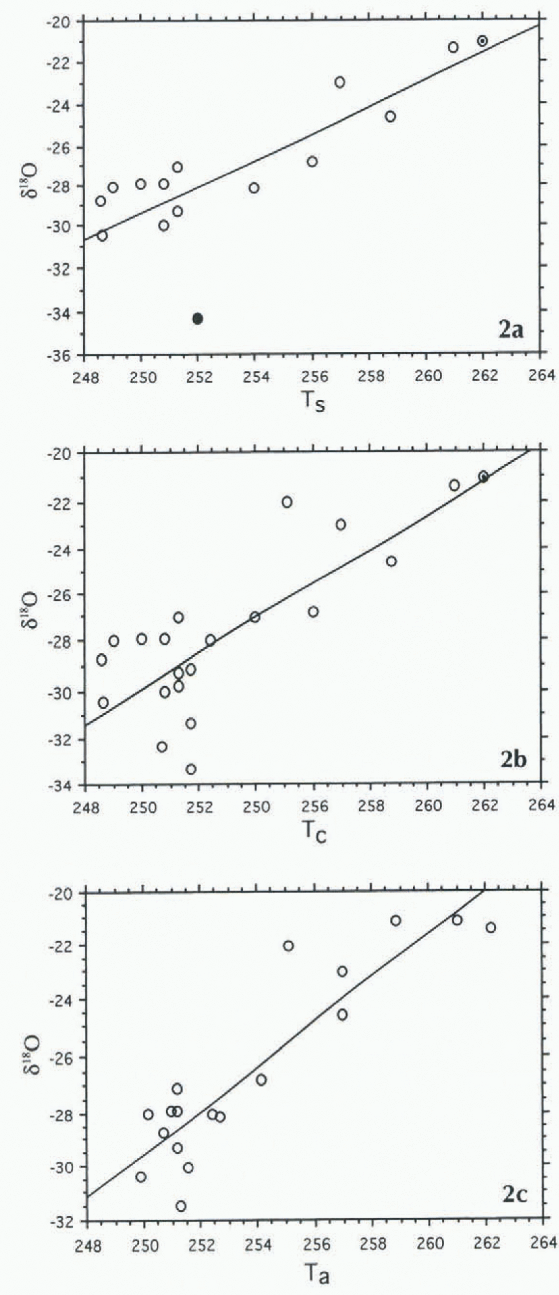
Fig. 2. (a) Scattergram for N16,δ¹⁸O = f(T_s).The full circle depicts data for site 13; the dot and circle indicate data for two sites. (b) Scattergram for N22,δ¹⁸O = f(T_c). Site 13is excluded; the dot and circle indicate two sites. (c) Scatter-gram for N22, δ¹⁸O = f(T_a). Site 13 is excluded.

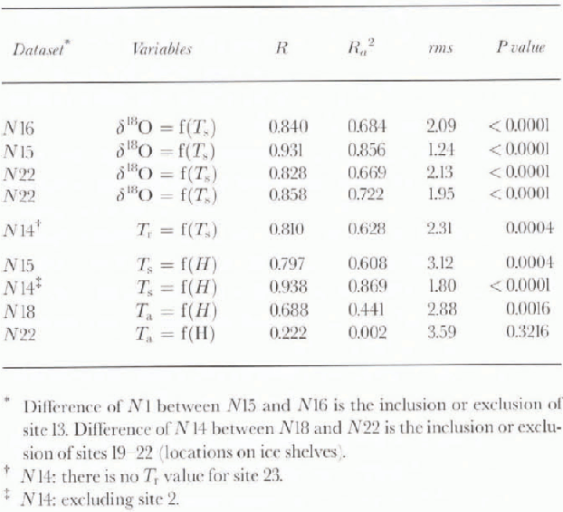
Table 2. Summary of bivariate regression analyses

A comparison of T _s, and T _r, including sites for which these data are available, showed a moderate correlation (N14; R is 0.810, R_a ² is 0.628, rms is 2.31. P is 0.0004), whereas similar comparisons in Antarctica and Greenland result in strong correlations (R values of 0.978 and 0.966, re-spectively (Reference Giovinetto and ZwallyGiovinetto and Zwally, 1997; Reference Zwally and GiovinettoZwaIly and Giovinetto, 1997)). The moderate correlation obtained for a region where topography, surface material, surface slope orientation, and lower troposphcric flow are more complex than on the ice sheets, support the use of T _r values for the remaining seven sites.

There is a slight weakening of the correlation between δ¹⁸O and lemperature relative to that obtained from the N15 set when it is enlarged by the introduction of T _r, Values for seven sites (Table 1. T _c; Fig. 2): N22, δ¹⁸O = f(T _c), R is 0.828. R_a ² is 0.669, rms is 2.13. The weakening of the correlation may be explained all or in part by uncertainties in the T _s and T _r data, mentioned above.

In an attempt to reduce uncertainties in the determination of T _s and T _r values, we entered the mean of T _s and T _r where possible, otherwise we entered T _r (Table 1: T _a). The scattergram of δ¹⁸O = f(T _a) based on the N22 dataset (Fig. 2; R is 0.858, R_a ² is 0.722. rms is 1.95):

(2)

illustrates the principal part of the model eventually selected as best.

It should be noted, however, that all of the following analyses were carried out in the N15, N16 and N22, N23 sets (i.e. including and excluding data from site 13, as well as for datasets using either T _s or T _a). For brevity, we report only on the basis of the best stepwise model obtained from the N22 set, although the best multiple regression model was obtained from the N15 set (Table 3: largest values of R at 0.951 and R_a ² at 0.867, smallest rms is 1.19):

(3)

The multivariate model obtained from the N22 set produces the second largest values of R at 0.915 and R_a ² 0.798, and second smallest rms is 1.67):

(4)

Stepwise analysis of the larger dataset should establish which independent variable or variables do not contribute significantly to the explanation of variation.

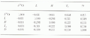
The descriptive statistics for the N22 set using T _a data (Table 4) show the range of each variable represented in the models.The correlation matrix (Table 5) lists the strong correlation between δ¹⁸O and T _a already mentioned (R is 0.858), and it shows from weak to no correlation between any other pair of variables.

In most cases there are obvious explanations for the lack of correlation. For example, between temperature and elevation, we obtained a moderate correlation using T _s (N15; R is 0.797, R_a ² is 0.608, rms is 3.12, P is 0.0004); the data for site 2 showed a departure >3 rms from The regression line, and when excluded, the correlation improved significantly (Fig. 3. N14; R is 0.938, R_a ² is 0.869, rms is 1.80. P is 0.0001). However, using T _a for all sites other than sites 19–22 located on ice shelves, the correlation decays significantly (Fig. 3, N18; R is 0.688, R_a ² is 0.441. rms is 2.88, P is 0.0016). and if these sites are included there is no correlation (N22; R is 0.222, P is 0.3216). The data from the ice shelves would form a cluster outside the elevation scale of Figure 3 (not shown, at H = 10 m, T_a ∼ 251 K) that lies >3 rms from the regression line fitted to the N18 set.

Fig. 3. Srattergram for Nl8, T_a = f(H). Sites 13 and 19–22 are excluded; dot and circle indicate two sites. The dashed line corresponds to N14, T_s = f(H); it excludes sites 2 and 13.

Table 3. Summary of multiple regression analyses (δ¹⁸O as the dependent variable)

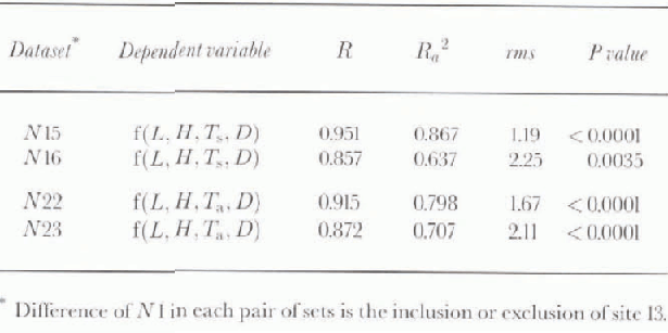
Table 4. Descriptive statistics (N22)

Table 5. Correlation matrix (N22)

Stepwise Analysis

Stepwise analysis of set N22 of The form δ¹⁸O = f(L, H, T_a, D) at the 99.9% confidence level show that T _a would be the only variable to enter the model in the forward mode (Table 6: R is 0.858, R_a ² is 0.722, rms is 1.95). The same result is obtained in the backward mode, in which the variables are removed in the following order: H, D, L. At the 95% confidence level, T _a enters the model first. H second while L and D do not enter (R is 0.883, R_a ² is 0.809, rms is 1.65). Runs at the 90% confidence level in cither the forward or backward mode did not show any changes.

Table 6. Summary of stepwise regression analyses (N22; δ¹⁸O as the dependent variable)

The best model produced using the N22 set in the backward mode at the 95% confidence level is:

(5)

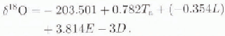
This model is similar to that obtained from Greenland data for 46 sites (Reference Zwally and GiovinettoZwally and Giovinetto, 1997), also at the 95% confidenee level in the backward mode (R is 0.987, R_a ² is 0.973, rms is 0.53):

(6)

where T _s, L and D, have the same units and were obtained on the same basis described in this study. It is remarkable that the intercept and temperature coefficient values in Equations (5) and (6) are close, although the Greenland data are, for the most part, representative of central and southern regions, rather than northwestern part.

Discussion and Conclusions

Our findings indicate that despite the relatively small data-set available to study the areal distribution of δ¹⁸O in northeastern Canada, it is possible to define a multivariate model at an acceptable confidence level. Moreover, The model may be used to produce a contoured pattern based on mean annual surface temperature, latitude and mean annual shortest distance to open ocean, ignoring the effects of surface elevation.

Inversion of Equation (5) produces ratio values (δ¹⁸O)_i, Table 1) that illustrate local differences between observation and model [(δ¹⁸O) – (δ¹⁸O)_i]. The difference is largest, as expected, for the location on Axel Heiberg Island that was excluded from most analyses (site 13, −5.98%₀). For the 22 sites used in the final analysis, the mean difference and sid dev. are −0.11 ± 1.50%₀, with a range −3.60–3.05%₀ (sites 16 and 18, respectively, both on Devon Island). The difference is smallest for the location on the Penny Ice Cap (site 2, −00.08%₀). This is of interest because, together with the difference for the location on the Barnes Ice Cap (site 23, l.00%₀), the two sites lie farthest south and away from the cluster to the north, indicating that the model is valid for a large area.

Our data compilation is not suitable to examine the variation of δ¹⁸O relative to elevation (e.g. over the area of a single ice cap). Nevertheless, it provides the basis to assess why elevation does not contribute to particular stepwise models. As listed in Table 1, the δ¹⁸O and H values show no correlation (N22; R <0.1, P >0.9). Exclusion of the data for ice shelves (sites 19–22) improves the correlation (N18 R is 0.758, P is 0.0003). However, the variation over a relatively small area requires using residual δ¹⁸O values produced in three steps, at each one removing the partial variation explained by L, D and T _a, respectively. There is no correlation between the δ¹⁸O residuals produced at the third step and H (N18; R <0.3, P >0.2).

The best δ¹⁸O predictive model described for northeastern Canada (Equation (5)) is similar to the best predictive model described for Greenland (Equation (6)), the latter based largely on data from its central and southern regions for which the principal sources of advected moisture are the North Atlantic sector extending from the Labrador Sea to the Norwegian Sea and waters to the south. This suggests that the bulk of The precipitation in Canada sampled by the sites compiled tor this study may share moisture advected from that sector.

The description of the sector must be qualified in that it is based on the mean annual position of the 10% sea-ice concentration boundary. If shortest distance to open ocean is measured using the mean annual position of the 50% concentration boundary, the description of the sector could be stated as extending from Baffin Bay to the Greenland Sea and waters to the south and east. In any event, the suggestion fits the findings of a detailed study on the origin of Arctic precipitation (Reference Johnsen, Dansgaard and WhiteJohnsen and others, 1989).