2.1. Governing equations and DNS datasets

The ZPG turbulent boundary layers are considered, as illustrated in figure 1. Assuming a calorically perfect gas, the zero-equation RANS equations are written as

(2.1a)$$\begin{gather} \frac{\partial \bar{\rho}}{\partial t} + \boldsymbol{\nabla} \boldsymbol{\cdot}\left(\bar{\rho} \tilde{\boldsymbol{u}}\right) = 0, \end{gather}$$

(2.1b) $$\begin{gather}\bar{\rho} \left(\frac{\partial \tilde{\boldsymbol{u}}}{\partial t} + \tilde{\boldsymbol{u}} \boldsymbol{\cdot}\boldsymbol{\nabla} \tilde{\boldsymbol{u}}\right) ={-}\boldsymbol{\nabla} \bar{p} + \boldsymbol{\nabla} \boldsymbol{\cdot} \left[ \left(\tilde{\mu} + \mu_t\right) \left( {\boldsymbol{\nabla} \tilde{\boldsymbol{u}} + \boldsymbol{\nabla} \tilde{\boldsymbol{u}}^{\text{T}}} \right) \right] - \frac{2}{3} \boldsymbol{\nabla} \left[ \left(\tilde{\mu}+\mu_t\right) \boldsymbol{\nabla} \boldsymbol{\cdot} \tilde{\boldsymbol{u}} \right],\end{gather}$$

(2.1c) $$\begin{gather} \bar{\rho} c_p \bigg(\frac{\partial \tilde{T}}{\partial t} + \tilde{\boldsymbol{u}} \boldsymbol{\cdot}\boldsymbol{\nabla} \tilde{T} \bigg) - \left(\frac{\partial \bar{p}}{\partial t} + \tilde{\boldsymbol{u}} \boldsymbol{\cdot}\boldsymbol{\nabla} \bar{p} \right)\nonumber\\ = \left(\tilde{\mu}+\mu_t\right) \Big[ \boldsymbol{\nabla} \tilde{\boldsymbol{u}} \boldsymbol{:} \left( {\boldsymbol{\nabla} \tilde{\boldsymbol{u}} + \boldsymbol{\nabla} \tilde{\boldsymbol{u}}^{\text{T}}} \right) - \frac{2}{3} \left( {\boldsymbol{\nabla} \boldsymbol{\cdot} \tilde{\boldsymbol{u}}} \right)^2 \Big] + \boldsymbol{\nabla} \boldsymbol{\cdot}[\left(\tilde{\kappa} + \kappa_t\right) \boldsymbol{\nabla} \tilde{T}], \end{gather}$$

where $\rho$, $\boldsymbol {u}$, $T$ and $p=\rho RT$ are the fluid's density, velocity, temperature and pressure; $R$ and $c_p$ are the gas constant and isobaric specific heat; $\mu$ and $\kappa$ are molecular viscosity and thermal conductivity. The Reynolds and Favre averages are denoted as $\bar {\phi }$ and $\tilde{\phi }$ (fluctuations as $\phi ^{\prime }$ and $\phi ^{{\prime \prime }}$), respectively. The quantities $\mu _t$ and $\kappa _t$ model the Reynolds stress $-\bar {\rho }\widetilde{\boldsymbol {u}^{{\prime \prime }}\boldsymbol {u}^{{\prime \prime }}}$ and turbulent heat flux $-\bar {\rho }c_p \widetilde{\boldsymbol {u}^{{\prime \prime }} T^{{\prime \prime }}}$, whose formulations are described in § 2.3. The wall is set no-slip and isothermal or adiabatic. The variables in wall viscous units are expressed with a superscript $+$, as $\boldsymbol {x}^+={\boldsymbol {x}}/{\delta _\nu }$, $\bar {\rho }^+=\bar {\rho }/\rho _w$, $\tilde{\boldsymbol u}^+=\tilde{\boldsymbol u}/{u_\tau }$ and $\tilde {\mu }^+=\tilde {\mu }/\mu _w$, where $w$ represents the wall variables, $\delta _\nu =\mu _w/(\rho _w u_\tau )$ is the viscous length unit, $u_\tau =(\tau _w/\rho _w)^{1/2}$ is the friction velocity, $\tau _w$ is the wall shear. Correspondingly, the friction Reynolds number is ${\textit {Re}}_\tau =\delta _{99}/\delta _v$ with $\delta _{99}$ the nominal thickness based on streamwise velocity. Furthermore, semilocal units are adopted, with a superscript $*$ as $u_\tau ^*=(\tau _w/\bar {\rho })^{1/2}$, $\delta _\nu ^*=\tilde {\mu }/(\bar {\rho } u_\tau ^*)$, so $y^*=y/\delta _v^*$. Most recent transformations are based on $y^*$, so $y^*$ as the inner scaling can be used to classify different layers, in analogy to $y^+$ in incompressible flows. Besides, two commonly used Reynolds numbers are ${\textit {Re}}_\theta =\rho _\infty U_\infty \theta /\mu _\infty$ and ${\textit {Re}}_{\delta _2}=\rho _\infty U_\infty \theta /\mu _w$ (Fernholz & Finley Reference Fernholz and Finley1980), where $\theta$ is the momentum thickness and $\infty$ denotes free stream variables.

Figure 1.

Schematic of the compressible flat-plate ZPG boundary layers.

To comprehensively examine the modified BL model, wide elaborated DNS databases are employed for ZPG boundary layers from different sources, with ${\textit {Ma}}_\infty$ from 2 to 14 under adiabatic, cold and heated walls. The published data are from Pirozzoli & Bernardini (Reference Pirozzoli and Bernardini2011, Reference Pirozzoli and Bernardini2013), Zhang et al. (Reference Zhang, Duan and Choudhari2018) and Volpiani, Bernardini & Larsson (Reference Volpiani, Bernardini and Larsson2018, Reference Volpiani, Bernardini and Larsson2020), as summarized in table 1. Though ${\textit {Ma}}_\infty =14$ is reached, the high-enthalpy effects (e.g. Chen et al. Reference Chen, Xi, Ren and Fu2022b) are not considered following the reference set-up. Besides, the incompressible data from Schlatter & Örlü (Reference Schlatter and Örlü2010) are included, as a reference for the incompressible BL model. The viscous parameters in each case are computed according to the references. The viscosity is from Sutherland's law, the power law or the formula for $\rm {N}_2$ (the working fluid in case ZDC-M8Tw048R20). Constant ${\textit {Pr}}=c_p\mu /\kappa$ are adopted for the thermal conductivity.

Table 1.

Parameters for the DNS datasets, where $T_r$ is the recovery temperature ($T_w=T_r$ for adiabatic cases). The cases with multiple streamwise locations are labelled in the brackets of the case numbers. The abbreviations for data sources are used hereinafter, as SO for Schlatter & Örlü (Reference Schlatter and Örlü2010), PB for Pirozzoli & Bernardini (Reference Pirozzoli and Bernardini2011, Reference Pirozzoli and Bernardini2013), ZDC for Zhang et al. (Reference Zhang, Duan and Choudhari2018) and VBL for Volpiani et al. (Reference Volpiani, Bernardini and Larsson2018, Reference Volpiani, Bernardini and Larsson2020). The notation expresses ${\textit {Ma}}_\infty$, $T_w/T_r$ and ${\textit {Re}}_{\delta _2}$ (divided by 100).

Notably, (2.1) is expressed using the Favre-averaged variables (except for $\bar {\rho }$) to form a closed system (Gatski & Bonnet Reference Gatski and Bonnet2013). The difference between the Reynolds- and Favre-averaged results cannot be accounted for using the algebraic RANS models, so we simply use the Favre averages throughout for consistency of notation, though the DNS data mostly adopt the Reynolds averages. This simplification will not affect the main conclusions of this work because even for the M14Tw018R24 case of the highest ${\textit {Ma}}$, there are only slight differences between the DNS statistics from these two averages (Zhang et al. Reference Zhang, Duan and Choudhari2018).

2.2. Solution of boundary layer equations

Based on the hypersonic interaction parameter (White Reference White2006), the effects of shock-boundary-layer interaction at the leading edge are evaluated to be minor on the downstream locations for the cases in table 1. Therefore, the boundary layer equations can be used for efficient computation of the mean flow, in the absence of impinging shock and separation. From (2.1), the boundary layer equations are written as (e.g. White Reference White2006)

(2.2) \begin{equation} \left. \begin{gathered} \dfrac{\partial ( {\bar{\rho} \tilde{U}} )}{\partial x} + \dfrac{\partial ( {\bar{\rho} \tilde{V}} )}{\partial y} = 0,\\ \bar{\rho} \bigg( {\tilde{U} \dfrac{\partial \tilde{U}}{\partial x} + \tilde{V} \dfrac{\partial \tilde{U}}{\partial y}} \bigg) ={-} \dfrac{{\mathrm{d}} P_e}{{\mathrm{d}}\kern0.7pt x} + \dfrac{\partial }{\partial y} \bigg[ \left({\tilde{\mu} + \mu_t}\right) \dfrac{\partial \tilde{U}}{\partial y} \bigg],\\ \bar{\rho} c_p \bigg( {\tilde{U} \dfrac{\partial \tilde{T}}{\partial x} + \tilde{V} \dfrac{\partial \tilde{T}}{\partial y}} \bigg) = \tilde{U} \dfrac{{\mathrm{d}} P_e}{{\mathrm{d}}\kern0.7pt x} + \left({\tilde{\mu} + \mu_t}\right) \bigg( {\dfrac{\partial \tilde{U}}{\partial y}} \bigg)^2 + \dfrac{\partial }{\partial y} \bigg[ {\left( {\tilde{\kappa} + \kappa_t} \right) \dfrac{\partial \tilde{T}}{\partial y}} \bigg], \end{gathered} \right\} \end{equation}

where $\tilde{U}$ and $\tilde{V}$ are the streamwise ($x$) and wall-normal ($y$) velocities. The pressure is assumed invariant along the $y$-direction ($P_e$), so $\bar {\rho }=\rho _e T_e/\tilde{T}$ is satisfied, where $e$ denotes values at the boundary layer edge. More general formulations accounting for geometrical curvature, far-field shock and cross-flow can be found in Degani & Schiff (Reference Degani and Schiff1983) and Gupta et al. (Reference Gupta, Lee, Zoby, Moss and Thompson1990).

Due to the complex formulation of $\mu _t$ and $\kappa _t$ (§ 2.3), the boundary layer profiles are not self-similar, even with ZPG. To solve the non-self-similar flow, the Mangler–Levy–Lees transformation can be used to remove the singularity at the leading edge $x=0$ (Probstein & Elliott Reference Probstein and Elliott1956). The transformed coordinate $(\xi,\eta )$ is defined as

(2.3a,b)\begin{equation} {\mathrm{d}} \xi = \rho_e \mu_e U_e \,{\mathrm{d}}\kern0.7pt x, \quad {\mathrm{d}} \eta = \frac{\bar{\rho} U_e}{\sqrt{\xi}} \,{\mathrm{d}} y. \end{equation}

The continuity equation is then eliminated and the transformed momentum and energy equations are

(2.4a)$$\begin{gather} \xi \left({ F \dfrac{\partial F}{\partial \xi} - \dfrac{\partial F}{\partial \eta} \dfrac{\partial \varPi}{\partial \xi} }\right) = C_1 \dfrac{\partial^2 F}{\partial \eta^2} + \left({ \dfrac{\partial C_1}{\partial \eta} + \dfrac{\varPi }{2} }\right) \dfrac{\partial F}{\partial \eta} + ({ G - F^2 }) \dfrac{\xi}{U_e} \dfrac{{\mathrm{d}} U_e}{{\mathrm{d}} \xi}, \end{gather}$$

(2.4b)$$\begin{gather}\xi \left({ F \dfrac{\partial G}{\partial \xi} - \dfrac{\partial \varPi}{\partial \xi} \dfrac{\partial G}{\partial \eta} }\right) = C_2 \dfrac{\partial^2 G}{\partial \eta^2} + \left({ \dfrac{\partial C_2}{\partial \eta} + \dfrac{\varPi}{2} }\right) \dfrac{\partial G}{\partial \eta} + {\textit{Ec}}_e C_1 \left({ \dfrac{\partial F}{\partial \eta} }\right)^2, \end{gather}$$

where the normalized streamwise velocity and temperature are $F=\tilde{U}/U_e$ and $G=\tilde{T}/T_e$ and $\varPi =\int F\,{\mathrm {d}}\eta$. The other parameters are $C_1=\bar {\rho }(\tilde {\mu }+\mu _t)/(\rho _e\mu _e)$, $C_2=\bar {\rho }(\tilde {\kappa }+\kappa _t)/(\rho _e c_p \mu _e)$ and the Eckert number ${\textit {Ec}}_e=U_e^2/(c_pT_e)$. The streamwise pressure gradient is reflected in ${\mathrm {d}} U_e/{\mathrm {d}} \xi$ through the Bernoulli equation, taken to be zero in the flows considered. The wall-normal boundary conditions at the wall and in the free stream are

(2.5) \begin{equation} \left. \begin{array}{ll@{}} F=0, \quad G=T_w/T_e \text{ (isothermal) or } {\partial G}/{\partial \eta}=0 \text{ (adiabatic)}, & \text{at }\eta=0,\\ F\rightarrow 1, \quad G\rightarrow 1, & \text{at }\eta\rightarrow\infty. \end{array} \right\} \end{equation}

Equation (2.4) is solved using the streamwise marching procedure (Blottner Reference Blottner1963; Chen, Wang & Fu Reference Chen, Wang and Fu2021). At $\xi =0$, (2.4) degenerates into two ODEs in terms of $\eta$, which are solved using the shooting method and serve as the initial profile. Afterwards, the solution at $\xi >0$ is feasible through streamwise marching. The streamwise ($\xi$) derivatives are discretized using the third-order finite-difference scheme. The Chebyshev collocation method is adopted for the wall-normal direction ($\eta$), with more points clustering near the wall. A grid number $N_y=241$ is adequate to provide grid-independent results. A uniform $\xi$ mesh is adopted, while the grid with increasing spacing can be used for better robustness. At each $\xi _i$, Newtonian iteration is used for quick convergence of the nonlinear equations. Second-order convergence can be realized for laminar flows (e.g. Chen, Wang & Fu Reference Chen, Wang and Fu2022a), while for turbulent flows here, the derivatives of $\mu _t$ and $\kappa _t$ may not be smooth (due to the maximum and intersection functions, see § 2.3), so the convergence is only first order. The convergence criterion for $[F,G]^{\textrm {T}}$ is set to $10^{-9}$ and at most 50 iterations are allowed at each streamwise location. The above procedure is substantially more efficient than solving (2.1). For the cases in table 1, the mean flow at the target $x$ can be obtained within minutes on a desktop computer. The solver is verified (detailed in Appendix A) through comparing with Hendrickson et al. (Reference Hendrickson, Subbareddy, Candler and Macdonald2023), who solved the full Navier–Stokes (NS) equation with BL models using the US3D code.

It is worth mentioning that $\mu _t$ and $\kappa _t$ from the BL model are zero at $\xi =0$ (since $y=0$), so the initial profile at $\xi =0$ is exactly the laminar counterpart. Thereby, there is a numerical (not physical) transition process downstream as $\mu _t$ increases. If the transition is not desirable, the start point for marching $\xi _0$ can be placed somewhere downstream, where the maximum $\mu _t/\mu _\infty$ is already high and the flow is turbulent. The initial profile at $\xi _0>0$ can still be obtained by solving the ODEs with the streamwise derivatives (left-hand sides in (2.4)) artificially dropped. The regime of streamwise adjustment is short due to the parabolic nature of (2.2), so the results downstream are not sensitive to $\xi _0$.

2.3. Baseline BL model

As mentioned in § 1, the BL model using semilocal units for the inner layer construction outperforms the one using wall-viscous units in high-speed applications (Dilley & McClinton Reference Dilley and McClinton2001). Therefore, the semilocal version is selected as the baseline BL model for modification. For future reference, it is termed the BL-local model in this work. The formulations are specified below, primarily following Cheatwood & Thompson (Reference Cheatwood and Thompson1993) for the LAURA code. The two-layer formulation of $\mu _t$ in BL (and also CS) is

(2.6) \begin{equation} \mu_t = \left\{ \begin{array}{@{}ll} \mu_{t,i}, & y \le y_{m\mu}, \\ \mu_{t,o}, & y > y_{m\mu}, \end{array} \right. \end{equation}

where $y_{m\mu }$ is the matching (intersection) point between the inner layer ${\mu _{t,i}}$ and outer layer ${\mu _{t,o}}$. The former is based on the mixing length concept, as

(2.7a–c)\begin{equation} \mu_{t,i} = \bar{\rho} l_{mix}^2 \left| \tilde{\omega} \right|, \quad l_{mix} = \kappa_c y \left[ {1 - \exp \left( { - \frac{y^*}{A^+}} \right)} \right], \quad {A^+} = \frac{26}{\sqrt{|\bar{\tau}^+|}}, \end{equation}

where $\tilde{\omega }$ is the vorticity, $l_{mix}$ is the mixing length corrected by the exponential damping function of van Driest (Reference van Driest1956) and $\kappa _c$ is the von Kármán constant, taken as 0.40. There are two differences in (2.7a–c) from the original version of Baldwin & Lomax (Reference Baldwin and Lomax1978). First, $y^*$ is used in the exponent of $l_{mix}$, instead of $y^+$, which was also adopted in recent works on WMLES (Yang & Lv Reference Yang and Lv2018; Fu, Bose & Moin Reference Fu, Bose and Moin2022; Kamogawa, Tamaki & Kawai Reference Kamogawa, Tamaki and Kawai2023). Second, $A^+$ is not a constant, but dependent on the local total shear $\bar {\tau }^+=\bar {\tau }/\tau _w$. For thin layer flows, $|\tilde{\omega }|$ can be simplified to $|{\partial \tilde{U}_{{\scriptscriptstyle /\!/}}}/{\partial n}|$, where $\tilde{U}_{{\scriptscriptstyle /\!/}}$ is the velocity parallel to the wall, and $n$ is the wall-normal direction. For the configurations in figure 1, we simply have $|\tilde{\omega }|=|{\partial \tilde{U}}/{\partial y}|$.

The outer-layer viscosity is evaluated by the Clauser–Klebanoff formulation (Klebanoff Reference Klebanoff1955; Clauser Reference Clauser1956). First, Clauser reasoned that for boundary layers, the eddies sufficiently away from the wall are no longer constrained by the wall, so their sizes should be proportional to the overall boundary layer thickness. The resulting maximum kinematic eddy viscosity in the outer layer is $\nu _{t,max}\sim U_e \delta _k^*$, or $\nu _{t,max}=\alpha U_e \delta _k^*$, where $\delta _k^*=\int (1-\tilde{U}/U_e)\,{\mathrm {d}} y$ is the kinematic displacement thickness (equals the displacement thickness in incompressible cases) and $\alpha$ is a closure coefficient. Farther away from the wall, the flow becomes intermittent. An empirical intermittency factor $F_{{Kleb}}$ (specified later) was introduced by Klebanoff, to model the diminishing of $\nu _{t,o}$ with increasing height. Consequently, $\mu _{t,o}$ is computed as $\bar {\rho }\nu _{t,max}F_{{Kleb}}$, which leads to the prevailing CS model. To avoid determining the boundary layer thicknesses, which is beneficial for complex flows, $U_e \delta _k^*$ in $\nu _{t,max}$ is replaced by the wake function $C_{cp} y_{max} F_{max}$ in the BL model, which can be justified from the defect velocity scaling (detailed in § 3.2). Therefore, the outer-layer $\mu _t$, adopted without explicit compressible corrections, is

(2.8)\begin{equation} \mu_{t,o} = \bar{\rho} \alpha C_{cp} y_{max} F_{max} F_{{Kleb}}, \end{equation}

where the vorticity function and the intermittency function are

(2.9a,b)\begin{equation} F_{max} = \frac{1}{\kappa_c} \max_{y=y_{max}} \left({l_{mix} \left| \tilde{\omega} \right| }\right), \quad F_{{Kleb}} \left({ \frac{y}{y_{max}} }\right) = \bigg[{ 1 + 5.5 {{\bigg({ C_{{Kleb}} \frac{y}{y_{max}} }\bigg)}^6} }\bigg]^{{-}1}. \end{equation}

Notably, $y_{max}$ is the peak position of the vorticity function following common usage, not the height of the computational domain. Compared with the CS model, the boundary layer thickness in $F_{{Kleb}}$ is replaced by $y_{max}/C_{{Kleb}}$. For more general flows, $\mu _{t,o}$ can be further restricted by a wake relation designed for free shear flows (see Wilcox Reference Wilcox2006). It is inactive in the present wall-bounded cases, thus not displayed for conciseness.

Besides $\kappa _c$ and $A^+$, there are three closure coefficients $\alpha$, $C_{cp}$ and $C_{{Kleb}}$ in the baseline model. Some works (e.g. Gupta et al. Reference Gupta, Lee, Zoby, Moss and Thompson1990) suggest their ${\textit {Ma}}$ dependence, but following the principles in § 1, we adopt the original constant values, $\alpha =0.0168$, $C_{cp}=1.6$ and $C_{{Kleb}}=0.3$. After the numerical discretization, the intersection and maximum operations in (2.6) and (2.9a,b) are conducted after a third-order interpolation on adjacent grid points, to ensure smoothness and accuracy. After obtaining $\mu _t$, $\kappa _t=c_p\mu _t/{\textit {Pr}}_t$ is calculated through a prescribed ${\textit {Pr}}_t$. Although ${\textit {Pr}}_t$ can be designed as a function of the wall-normal height (Subbareddy & Candler Reference Subbareddy and Candler2012), the simplest choice of a constant ${\textit {Pr}}_t$ is adopted, equal to 0.9 as a common choice. The effects of ${\textit {Pr}}_t$ variations will be discussed in § 3.3.

Two cases are employed to demonstrate the behaviour of the baseline BL-local model. First is an incompressible case from SO (${\textit {Ma}}_\infty$ set to 0.01 in our solver). The mean velocity and eddy viscosity are compared with the DNS data at ${\textit {Re}}_\theta =2540$ in figure 2. Note that $\mu _t$ from DNS is evaluated by definition as $\mu _t=-\bar {\rho }\widetilde{u^{{\prime \prime }} v^{{\prime \prime }}}/(\partial \tilde{U}/\partial y)$; $\mu _t$ near the boundary layer edge is not displayed since both the numerator and denominator tend to zero. The predicted streamwise velocity is basically in line with DNS, showing the good capability of BL for incompressible flows. In the inner layer, $\mu _t^+$ faithfully follows the incompressible scaling by Johnson & King (Reference Johnson and King1985) as

(2.10)\begin{equation} \nu_{t,i}^+= \kappa_c y^+ \left[1 - \exp \left( -\frac{y^+}{17} \right) \right]^2, \end{equation}

where the last multiplier is termed the damping function. Note that (2.10) is more convenient than (2.7a–c) for comparisons between cases because $\tilde{\omega }$ does not explicitly appear. Away from the wall, the damping function is nearly unity, so the logarithmic scaling is formulated. In the outer layer, the peak value $\mu _{t,max}=\bar {\rho }\nu _{t,max}$ from the BL model is also close to the DNS (note that $\bar {\rho }$ is invariant), so the matching point $y_{m\mu }^+=152$ ($\kern0.7pt y_{m\mu }=0.18\delta _{99}$) is near the upper bound of the logarithmic region, above which the outer-layer scaling is formulated. Although $\mu _{t,o}$ damps (by $F_{{Kleb}}$) more slowly than the DNS in the intermittent region, only a minor difference in $\tilde{U}$ appears due to the diminishing $\partial \tilde{U}/\partial y$.

Figure 2.

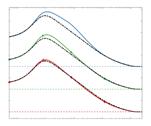
(a,c) Eddy viscosity and (b,d) mean streamwise velocity and temperature (only compressible case) from the baseline BL-local model and DNS for the (a,b) incompressible SO-M0R25 case and (c,d) hypersonic ZDC-M8Tw048R20 case.

For the hypersonic cold-wall case M8Tw048R20 from ZDC, however, $\tilde{U}$ and $\tilde{T}$ from the BL-local model have clear deviations from the DNS data, especially for $\tilde{T}$, as shown in figure 2(d). The discrepancy can be explained from figure 2(c). Compared with DNS, $\mu _{t,o}$ is severely underestimated, so the matching point $y_{m\mu }^*=67$ ($\kern0.7pt y_{m\mu }=0.09\delta _{99}$) is quite low. Consequently, the region $67< y^*\lesssim 300$ ($0.09< y_{m\mu }/\delta _{99}\lesssim 0.27$) is not formulated by the logarithmic scaling in (2.7a), leading to the errors in $\tilde{U}$ and $\tilde{T}$ there. Meanwhile, $\tilde{T}$ around the temperature peak ($\kern0.7pt y^*\sim 7$) is over-predicted, possibly due to the inaccurate ${\textit {Pr}}_t$ there (specified in § 3.3).

In the following, the inner and outer-layer scalings of $\mu _t$ and $\kappa _t$ are investigated separately using the DNS data. Three targeted modifications are proposed based on established relations.

3.1. Inner-layer scaling

First, we demonstrate that the formulation of $\mu _{t,i}$ in the BL-local model is equivalent to applying the TL transformation. Analogous derivation was presented by Yang & Lv (Reference Yang and Lv2018) within the WMLES framework. Using the definition of $\mu _t$ and (2.7a–c), the mixing-length relation can be expressed, in wall-viscous units, as

(3.1)\begin{equation} {-}\bar{\rho}^+ \widetilde{u^{{{\prime\prime}}+} v^{{{\prime\prime}}+}} = \bar{\rho}^+ l_{mix}^{{+}2} \bigg| \frac{\partial \tilde{U}^+}{\partial y^+} \bigg|^2 = \bar{\rho}^+ \bigg| \frac{\partial \tilde{U}^+}{\partial y^+} \bigg|^2 \kappa_c^2 y^{{+}2} \left[ {1 - \exp \left( { - \frac{y^*}{A^+}} \right)} \right]^2. \end{equation}

The left-hand side, $-\bar {\rho }^+ \widetilde{u^{{{\prime \prime }}+}v^{{{\prime \prime }}+}}=-\bar {\rho } \widetilde{u^{{{\prime \prime }}}v^{{{\prime \prime }}}}/\tau _w=-\widetilde{u^{{{\prime \prime }}*}v^{{{\prime \prime }}*}}$, is the density-weighted or semilocal Reynolds shear stress (Morkovin's scaling), which is known to well match the incompressible counterpart in the inner layer in terms of $y^*$ (Coleman et al. Reference Coleman, Kim and Moser1995; Pirozzoli & Bernardini Reference Pirozzoli and Bernardini2011; Zhang et al. Reference Zhang, Duan and Choudhari2018; Hirai, Pecnik & Kawai Reference Hirai, Pecnik and Kawai2021; Cheng & Fu Reference Cheng and Fu2022; Cogo et al. Reference Cogo, Salvadore, Picano and Bernardini2022; Bai et al. Reference Bai, Cheng, Griffin, Li and Fu2023). Meanwhile, it is recognized that the right-hand side is related to the TL transformation, $U_{{TL}}^+(\kern0.7pt y^*)= \int \bar {\mu }^+(\partial y^*/\partial y^+) \,{\mathrm {d}} \bar {U}^+$. The resulting form, under the notation of Favre averages, is

(3.2)\begin{equation} {-}\bar{\rho}^+ \widetilde{u^{{{\prime\prime}}+}v^{{{\prime\prime}}+}} = \bigg| \frac{\partial {U}_{{TL}}^+}{\partial y^*} \bigg|^2 \kappa_c^2 y^{*2} \left[ {1 - \exp \left( { - \frac{y^*}{A^+}} \right) }\right]^2. \end{equation}

The left-hand side and right-hand side are both functions of $y^*$, so if the transformed inner layer shear well matches the incompressible counterpart, then (2.7a) will be a highly accurate modelling of $\mu _{t,i}$. For diagnostic purposes, a semilocal eddy viscosity is defined as

(3.3)\begin{equation} \mu_{t,{{TL}}}^*(\kern0.7pt y^*) = \frac{-\bar{\rho}^+ \widetilde{u^{{{\prime\prime}}+}v^{{{\prime\prime}}+}}}{{\partial {U}_{{TL}}^+}/{\partial y^*}} = \frac{\mu_t}{\tilde{\mu}}, \end{equation}

which is expected to match the incompressible $\mu _{t,i}$ (or $\nu _{t,i}$). Equation (3.3) is examined in figure 3(a) using all the DNS data in table 1. Since we are concerned with the inner layer part, $\mu _{t,{{TL}}}^*$ is plotted in dotted lines after reaching its maximum. The reference line is the counterpart of (2.10) with $y^+$ replaced by $y^*$ (Yang & Lv Reference Yang and Lv2018), as

(3.4)\begin{equation} \mu_{t,i}^* = \kappa_c y^* \left[1 - \exp \left( -\frac{y^*}{17} \right) \right]^2. \end{equation}

There is only a small scattering of $\mu _{t,{{TL}}}^*(\kern0.7pt y^*)$ within and below the buffer layer, showing the accuracy of the TL transformation for that region. This also explains the well-predicted surface quantities in the BL-local model for hypersonic cases (Dilley & McClinton Reference Dilley and McClinton2001). In the logarithmic region, $\mu _{t,{{TL}}}^*$ tends to be lower than (3.4), especially for diabatic cases, suggesting an underestimated $\mu _{t,i}$ in BL-local. This is consistent with the behaviour of $U_{{TL}}^+$, which can lead to over-prediction in the logarithmic region in diabatic cases. Nevertheless, figure 2(c) indicates that $\mu _{t,i}$ in the BL-local model is somewhat higher than DNS, rather than lower. This inconsistency is due to the discrepancy in $\tilde{T}$, on which the variables for constructing the semilocal units ($\bar {\rho }$ and $\tilde {\mu }$) are dependent.

Figure 3.

Semilocal eddy viscosity using the (a) TL (as in the BL-local model) and (b) GFM transformations from the DNS datasets. The legends for panels (a,b) are the same, separately shown in the two boxes.

As an alternative, we employ the GFM transformation to construct $\mu _{t,i}$, a thought recently implemented by Griffin et al. (Reference Griffin, Fu and Moin2023) and Hendrickson et al. (Reference Hendrickson, Subbareddy, Candler and Macdonald2023) for model improvement. The results using the very recent HLPP transformation will be discussed in Appendix B. The GFM is shown to have better overall performances than TL for canonical air flows, particularly diabatic boundary layers in the logarithmic layer, though it can degrade for supercritical or non-air-like flows (Bai et al. Reference Bai, Griffin and Fu2022; Hasan et al. Reference Hasan, Larsson, Pirozzoli and Pecnik2023b). This transformation is defined as

(3.5a,b)\begin{align} U_{{GFM}}^+ (\kern0.7pt y^*) = \int_0^{y^*} S_t^+ \,{\mathrm{d}} y^*, \quad S_t^+= \frac{S_{eq}^+}{1 + S_{eq}^+- S_{TL}^+} = \frac{\dfrac{1}{\tilde{\mu}^+} \dfrac{\partial \tilde{U}^+}{\partial y^*}}{1 + \dfrac{1}{\tilde{\mu}^+} \dfrac{\partial \tilde{U}^+}{\partial y^*} - \tilde{\mu}^+ \dfrac{\partial \tilde{U}^+}{\partial y^+}}, \end{align}

where $S_{TL}^+$ is the TL transformation kernel defined above, and $S_{eq}^+$ results from the approximate balance of turbulence production and dissipation in the logarithmic region, as a modification to the arguments of Zhang et al. (Reference Zhang, Bi, Hussain, Li and She2012). Similar to (3.2), the GFM-based mixing length relation in the semilocal coordinate takes the form of

(3.6)\begin{equation} {-}\bar{\rho}^+ \widetilde{u^{{{\prime\prime}}+}v^{{{\prime\prime}}+}} = \bigg| \frac{\partial U_{{GFM}}^+}{\partial y^*} \bigg|^2 \kappa_c^2 y^{*2} \left[ {1 - \exp \left( { - \frac{y^*}{A^+}} \right)} \right]^2. \end{equation}

Accordingly, the semilocal eddy viscosity using GFM is

(3.7)\begin{equation} \mu_{t,{{GFM}}}^*(\kern0.7pt y^*) = \frac{-\bar{\rho}^+ \widetilde{u^{{{\prime\prime}}+}v^{{{\prime\prime}}+}}}{{\partial U_{{GFM}}^+}/{\partial y^*}} = \frac{\mu_t}{\tilde{\mu}} \frac{{\partial U_{{TL}}^+}/{\partial y}}{{\partial U_{{GFM}}^+}/{\partial y}}. \end{equation}

As shown in figure 3(b), $\mu _{t,{{GFM}}}^*$ experiences smaller scattering than $\mu _{t,{{TL}}}^*$ at $y^*\lesssim 70$. Also, $\mu _{t,{{GFM}}}^*$ in the logarithmic region follows (3.4) more closely, demonstrating better robustness for modelling $\mu _{t,i}$ than (2.7a). For practical use, the incompressible analogy $\mu _{t,{{GFM}}}^*$ is computed first using (3.6), based on $y^*$ and ${\partial {U}_{{GFM}}^+}/{\partial y^*}$; afterward, $\mu _{t,i}$ is obtained from (3.7).

Notably, the GFM and TL transformations are designed only for the region within and below the logarithmic layer, so their accuracy for the outer region is not guaranteed. Consequently, they may not be directly used to modify the outer-layer $\mu _t$. Our exploration to improve the $\mu _{t,o}$ modelling is presented below.

3.2. Outer-layer scaling

The derivation of the outer-layer scaling in the baseline BL model is briefly reviewed first, to set the grounds for possible modifications.

The crucial part of modelling $\mu _{t,o}$ is the estimation of its peak value, as learned from figure 2. In (2.8), the peak value $\nu _{t,max}$ is estimated first, then $\mu _{t,o}$ is formed as $\bar {\rho }\nu _{t,max}$ before the diminishing by $F_{{Kleb}}$. Consequently, $\mu _{t,o}$ can continue to increase at $y>y_{m\mu }$ due to the rising $\bar {\rho }$ (see figure 2c), rather than monotonically decreasing as in incompressible cases. Therefore, it is first a question whether $\nu _{t,max}$ (then $\mu _{t,o}=\bar {\rho }\nu _{t,max}F_{{Kleb}}$, as in BL-local) or $\mu _{t,max}$ (the maximum $\mu _t$, then $\mu _{t,o}=\mu _{t,max}F_{{Kleb}}$ which monotonically decreases with $y$) should be modelled. In hypersonic cases, $\bar {\rho }$ can vary considerably in the outer region, so the two strategies can lead to significant differences. From existing works, the scaling for $\mu _{t,max}$ is scarce while that for $\nu _{t,max}$ is prevailing, so the following investigation is mainly on $\nu _{t,max}$. As mentioned in § 2.3, Cebeci & Smith (Reference Cebeci and Smith1974) argued that $\nu _{t,max}$ was proportional to the boundary layer thickness, and suggested two scalings,

(3.8a,b)\begin{equation} \nu_{t,max}=\alpha U_e\delta_k^* = \alpha \nu_e {\textit{Re}}_{\delta_k^*} \quad \text{and} \quad \nu_{t,max}=\alpha_2 u_\tau \delta_{99} = \alpha_2 \nu_w {\textit{Re}}_{\tau}, \end{equation}

which also hold in compressible flows. The first closure constant $\alpha$ has been introduced in § 2.3, and the second one $\alpha _2$ is $0.06\unicode{x2013} 0.075$. Although widely used, (3.8) is re-examined here using the DNS data for future reference. The ratios $\alpha _{2,DNS}=\nu _{t,max}/(u_\tau \delta _{99})$ and $\alpha _{DNS}=\nu _{t,max}/(U_e \delta _k^*)$ for all cases are shown in figure 4(a,b), as functions of the corresponding Reynolds numbers. For incompressible cases, $\alpha _{2,DNS}$ varies more slightly than $\alpha _{DNS}$ with increasing ${\textit {Re}}$. When compressible cases are included, however, $\alpha _{2,DNS}$ is the less robust one. In particular, $\alpha _{2,DNS}$ varies more than twice between the diabatic cases, which is not surprising due to its higher sensitivity to wall quantities by definition.

Figure 4.

Maximum kinematic eddy viscosity scaled by different variables (see (3.8a,b) and (3.11)) from the DNS data. The diamonds are for incompressible cases, and the cycles and triangles are for adiabatic and diabatic ones, respectively. The symbol colours follow the usage in figure 3.

For incompressible flows, the well-known velocity defect law provides another way to estimate $\nu _{t,max}$ without using the boundary layer thicknesses, as adopted in the BL model. Specifically, the Clauser defect law reads $U_e^+-\tilde{U}^+=U_{{df}}^+(\eta )$, where $U_{{df}}^+$ is the defect velocity and the outer scale $\eta =y/\varDelta$ is based on the Rotta–Clauser boundary layer thickness $\varDelta =U_e^+\delta _k^*=\int (U_e^+-\tilde{U}^+)\,{\mathrm {d}} y$ (note that $\eta$ is no longer the transformed coordinate defined in § 2.2). Consequently, a collapse of the following function is suggested as

(3.9)\begin{equation} {-}\eta \frac{{\mathrm{d}} U_{{df}}^+}{{\mathrm{d}} \eta} = \eta \frac{\partial \tilde{U}^+}{\partial \eta} = y \frac{\partial \tilde{U}^+}{\partial y} \approx \frac{l_{mix}}{\kappa_c} \frac{\partial \tilde{U}^+}{\partial y} = \frac{l_{mix} \left| \tilde{\omega} \right|}{\kappa_c u_\tau} , \end{equation}

where the approximation holds in the outer layer where $y^*\gg A^+$ (see (2.7c)). The last term is the scaled vorticity function in (2.9a), and the first three terms are the diagnostic function commonly used to evaluate $\kappa _c$, though the main focus here is on the outer layer. For a quantitative evaluation of (3.9) and then $y_{max} F_{max}$, the semiempirical relation by Monkewitz, Chauhan & Nagib (Reference Monkewitz, Chauhan and Nagib2007) for incompressible boundary layers in the large-${\textit {Re}}$ limit is employed, which gives one explicit expression of $U_{{df}}^+(\eta )$. As a result, the outer-layer maximum of $y\partial \tilde{U}^+/\partial y$ is equal to 5.55 at $\eta =0.155$. Therefore, the ratio of $\nu _{t,max}$ to $y_{max} F_{max}$ using (3.8a), i.e.

(3.10)\begin{equation} \frac{\nu_{t,max}}{\alpha y_{max} F_{max}} = \frac{U_e \delta_k^*}{0.155 U_e^+\delta_k^* \times 5.55 u_\tau} = \frac{1}{0.155\times5.55}, \end{equation}

is a constant (namely $C_{cp}$, though not exactly the same value), which leads to (2.8) directly used in the compressible baseline BL model. Analogously, if $\nu _{t,max}$ is from (3.8b), then the constant in (3.10) can be obtained from another form of incompressible defect law $U_e^+-\tilde{U}^+=U_{{df}}^+(\kern0.7pt y/\delta _{99})$. Inspired by (3.9) and (3.10), the compressible defect velocity scalings and their derivatives are examined below, to explore possible compressible corrections to (2.8).

As introduced in § 1, most of the existing compressible defect velocity scalings are based on the VD transformation. The VD is built upon the mixing length assumption for the region within and below the logarithmic layer, so the outer layer is not the targeted region for it to work, like other transformations (TL, GFM, etc.). Nevertheless, previous investigations actively support its usage for compressible defect velocity scalings (Maise & McDonald Reference Maise and McDonald1968; Fernholz & Finley Reference Fernholz and Finley1980; Guarini et al. Reference Guarini, Moser, Shariff and Wray2000; Pirozzoli et al. Reference Pirozzoli, Grasso and Gatski2004; Duan et al. Reference Duan, Beekman and Martín2011; Pirozzoli & Bernardini Reference Pirozzoli and Bernardini2011; Wenzel et al. Reference Wenzel, Selent, Kloker and Rist2018), suggesting its fundamentality in transforming compressible flows, though the diabatic cases are somewhat insufficiently examined. Therefore, the VD transformation is considered until future reports of more advanced ones. Following the incompressible procedures above, a VD-based displacement thickness can be defined, following Smits & Dussauge (Reference Smits and Dussauge2006), as

(3.11)\begin{equation} \delta_{{{VD}}}^* = \int_0^\infty \left( 1-\frac{U_{{VD}}}{U_{{{VD}},e}} \right)\,{\mathrm{d}} y, \quad \text{where} \ U_{{VD}}^+ (\kern0.7pt y^+) = \int_0^{\tilde{U}^+} {\sqrt{\bar{\rho}^+}\,{\mathrm{d}} \tilde{U}^+}. \end{equation}

The corresponding outer scale is $\eta _{{VD}}=y/\varDelta _{{VD}}$, where the transformed Rotta–Clauser thickness is $\varDelta _{{VD}}=U_{{{VD}},e}^+\delta _{{{VD}}}^*=\int (U_{{{VD}},e}^+-U_{{VD}}^+)\,{\mathrm {d}} y$. Since VD may not be accurate enough in the inner layer, the transformed displacement thickness can be alternatively defined in a mixed manner, $\delta _{mix}^*$, where the integrand in the inner region (say $y<0.15\delta _{99}$) is replaced by the TL- or GFM-based defect velocity. Taking GFM as an example, the difference between $\delta _{mix}^*$ and $\delta _{{{VD}}}^*$ turns out to be less than 2.5 % and 4.5 % for the supersonic and hypersonic cases, respectively. Since $\delta _{\textit{VD} }^*$ is not finally used in the new model but to inform modification, we employ $\delta _{{{VD}}}^*$ instead of $\delta _{mix}^*$ hereafter for simplicity and consistency. Similar to (3.8), $\nu _{t,max}$ can be evaluated as $\nu _{t,max}=\alpha _{{{VD}}} U_e\delta _{{{VD}}}^*=\alpha _{{{VD}}} \nu _e {\textit {Re}}_{\delta _{{{VD}}}^*}$, which is examined in figure 4(c) by computing $\alpha _{VD,DNS}=\nu _{t,max}/(U_e\delta _{{{VD}}}^*)$ for all cases. The ratio $\alpha _{VD,DNS}$ experiences a comparably small variation with $\alpha _{DNS}$. Besides, there is generally a decreasing trend of $\alpha _{VD,DNS}$ with ${\textit {Re}}_{\delta _{{{VD}}}^*}$ rising, which awaits future examination using higher-${\textit {Re}}$ data. Notably, the diabatic cases exhibit no larger departure than the incompressible and adiabatic cases, though the VD transformation tends to deteriorate. A possible reason is that (3.11) is defined in an integral manner, allowing error cancellation.

Afterwards, the compressible defect velocity scalings are studied, to establish connections with the vorticity function. The form examined by Pirozzoli & Bernardini (Reference Pirozzoli and Bernardini2011) for supersonic adiabatic boundary layers is $(U_{{{VD}},e}-U_{{VD}})/U_{{{VD}},e}=g_1(\kern0.7pt y/\delta _{99})$, where $g_1$ is a universal function. This function is computed in figure 5(c) for all the DNS cases, and the results before the VD transformation are plotted in figure 5(a) for comparison. As can be seen, $g_1$ for diabatic cases deviates more significantly from the incompressible counterpart. As an alternative to $g_1$, the VD-based analogy to the Clauser defect law takes the form of $U_{{{VD}},e}^+-U_{{VD}}^+=g_2(\eta _{{VD}})$, which is examined in figure 5(b) between cases. For the present datasets, $g_2$ tends to achieve a somewhat better collapse than $g_1$. We proceed to study the derivatives of these defect velocities, to connect with the diagnostic function and then the vorticity function. The diagnostic function used in (2.8) is displayed in figure 5(d), where a few strongly oscillating curves are not shown. Note that $y{\partial \tilde{U}^+}/{\partial y}$ is plotted instead of $y{\partial \tilde{U}}/{\partial y}$ for direct connection with $\nu _{t,max}$ (see (3.10), there is a factor $u_\tau$ in (3.8) or $\varDelta$). The main focus is on the outer layer, so the region $y<0.15\delta _{99}$ is plotted in dotted lines. If the outer-layer peaks of $y{\partial \tilde{U}^+}/{\partial y}$ are collapsed between cases, then the ratio $\nu _{t,max}/(\kern0.7pt y_{max}F_{max})$ would be nearly invariant, which would then provide a robust modelling for $\mu _{t,o}$, as derived in (3.10) for incompressible cases. First, the incompressible cases in figure 5(d) suggest a rough outer-layer similarity at this ${\textit {Re}}$ range (${\textit {Re}}_\tau \gtrsim 400$, ${\textit {Re}}_{\delta _2}\gtrsim 1400$), though the collapse is not as close to perfect as in the large-${\textit {Re}}$ limit (Nagib, Chauhan & Monkewitz Reference Nagib, Chauhan and Monkewitz2007). For the compressible cases, the peak locations in figure 5(d) all concentrate around $0.7\delta _{99}$, but the maximums vary considerably, especially for some cold-wall cases, even if the low-${\textit {Re}}$ cases are excluded. Consequently, $\mu _{t,o}$ can be severely under-predicted, as is observed in figure 2(c). For the VD-based defect velocity $g_2(\eta _{{VD}})$, the outer-layer relation analogous to (3.9) is derived as

(3.12)\begin{equation} {-}\eta_{{VD}} \frac{{\mathrm{d}} g_2}{{\mathrm{d}} \eta_{{VD}}} = y \frac{\partial U_{{VD}}^+}{\partial y} = \sqrt{\bar{\rho}^+} y \frac{\partial \tilde{U}^+}{\partial y} \approx \sqrt{\bar{\rho}^+} \frac{l_{mix} \left| \tilde{\omega} \right|}{\kappa_c u_\tau}, \quad \text{where }y^*\gg A^+. \end{equation}

As noted by Smits & Dussauge (Reference Smits and Dussauge2006), (3.12) indicates a proper velocity scale in the outer layer to be $u_\tau /\sqrt {\bar {\rho }^+}$, which can be used to extend Coles’ law of the wake (Maise & McDonald Reference Maise and McDonald1968; Huang et al. Reference Huang, Bradshaw and Coakley1993; Hasan et al. Reference Hasan, Larsson, Pirozzoli and Pecnik2023a). Furthermore, the factor $\sqrt {\bar {\rho }^+}$ turns out to be fundamental to account for compressibility effects, and was suggested by Catris & Aupoix (Reference Catris and Aupoix2000) and Otero Rodriguez et al. (Reference Otero Rodriguez, Patel, Diez Sanhueza and Pecnik2018) to improve the eddy viscosity and diffusivity in sophisticated RANS models. The transformed function $y{\partial U_{{VD}}^+}/{\partial y}$ is plotted in figure 5(e) in terms of $\eta _{{VD}}$. Although obvious scattering in peak values and locations is still observable, better collapse is attained compared with figure 5(d), demonstrating the effectiveness of the VD density weighting.

Figure 5.

Different forms of (a–c) defect velocities and (d–f) diagnostic functions for all cases. The reference lines in panels (d–f) are from (3.10). The legends for all the panels are the same, separately shown in the three boxes.

Therefore, it is suggested that the VD-based vorticity function can be utilized in the outer layer scaling of the BL model, to replace the original one without compressible corrections. From (3.12), the vorticity function in (2.9a) is modified by simply adding a factor $\sqrt {\bar {\rho }^+}$ as

(3.13)\begin{equation} F_{{{VD}},max} = \frac{1}{\kappa_c} \max_{y=y_{{{VD}},max}} ({ \sqrt{\bar{\rho}} l_{mix} \left| \tilde{\omega} \right| }). \end{equation}

Here, the denominator $\sqrt {\rho _w}$ has been moved out of this function to combine with other factors in $\mu _{t,o}$, which does not affect the value of $y_{{{VD}},max}$. Consequently, (2.8) is modified to be

(3.14)\begin{equation} \mu_{t,o} = \frac{\bar{\rho}}{\sqrt{\bar{\rho}}} \alpha C_{cp} y_{{{VD}},max} F_{{{VD}},max} F_{{Kleb}} = \sqrt{\bar{\rho}} \alpha C_{cp} y_{{{VD}},max} F_{{{VD}},max} F_{{Kleb}}. \end{equation}

Here, the denominator $\sqrt {\bar {\rho }}$ can be interpreted as a compensation to the amplified vorticity function (3.13). The final form also turns out to reach a compromise between the modelling of $\nu _{t,max}$ and $\mu _{t,max}$, so $\mu _{t,o}\sim \bar {\rho }^{1/2}F_{{Kleb}}$ and $\nu _{t,o}\sim \bar {\rho }^{-1/2}F_{{Kleb}}$. As a natural consequence, (3.14) produces the same results as (2.8) for incompressible flows with constant density.

The empirical function $F_{{Kleb}}(\kern0.7pt y/y_{{{VD}},max})$ remains unmodified as in (2.9b) before acquiring more theoretical guidance. Also, the closure constants $\alpha$, $C_{cp}$ and $C_{{Kleb}}$ remain unaltered, consistent with the incompressible version. Finally, since the quantity $y_{{{VD}},max}/C_{{Kleb}}$ used in $F_{{Kleb}}$ represents an estimation of the boundary layer thickness, its relation to $\delta _{99}$ is examined in figure 5(f) by plotting the transformed function in terms of $y/\delta _{99}$. For most cases, $y_{{{VD}},max}/\delta _{99}$ is within 0.6–0.8, but it seems closer to the boundary layer edge than $y_{max}/\delta _{99}$, suggesting slower damping of $\mu _{t,o}$ in the intermittent region.

3.3. The TV relation

As stated in § 2.3, the eddy diffusivity in RANS models for temperature prediction is obtained mostly through a specified ${\textit {Pr}}_t$, whose one common definition is

(3.15)\begin{equation} {\textit{Pr}}_t = \frac{\widetilde{u^{{\prime\prime}} v^{{\prime\prime}}} (\partial \tilde{T} / \partial y)}{\widetilde{v^{{\prime\prime}} T^{{\prime\prime}}} (\partial \tilde{U} / \partial y)}. \end{equation}

It is widely shown that ${\textit {Pr}}_t$ is within 0.7–1.1 in most regions above the buffer layer and is typically equal to 0.85 in the logarithmic region, insensitive to ${\textit {Ma}}$, ${\textit {Re}}$ and wall cooling (Huang, Coleman & Bradshaw Reference Huang, Coleman and Bradshaw1995; Duan et al. Reference Duan, Beekman and Martín2010; Pirozzoli & Bernardini Reference Pirozzoli and Bernardini2011; Lusher & Coleman Reference Lusher and Coleman2022). However, ${\textit {Pr}}_t$ can experience complicated variations within and below the buffer layer, especially in cold-wall boundary layers, which is illustrated in figure 6(a) using the DNS data from ZDC. At $y^*\gtrsim 25$, three ${\textit {Pr}}_t$ are quite close to each other, slowly decreasing towards the boundary layer edge. Near the temperature peak, however, $\partial \tilde{T}/\partial y$ and $\widetilde{v^{{\prime \prime }} T^{{\prime \prime }}}$ both change signs, so ${\textit {Pr}}_t$ can be negative or even singular. This singularity is also observable in the adiabatic case M2p5Tw10R17, though very close to the wall ($\kern0.7pt y^*\approx 2$). Meanwhile, ${\textit {Pr}}_t$ between the singular point and the wall is generally lower than 0.5 for the three cases. The rapid variation of ${\textit {Pr}}_t$ can lead to prediction errors for the temperature peak, as discussed for figure 2(d). For further demonstration, figure 6(b) compares between three cases with different ${\textit {Pr}}_t$ using the BL-local model (case M8Tw048R20). At $y^*\gtrsim 100$, $\tilde{T}$ is quite insensitive to ${\textit {Pr}}_t$ but at $y^*\lesssim 100$, a continuous decrease of $\tilde{T}$ is observed with the drop of ${\textit {Pr}}_t$ due to enhanced turbulent heat flux. The case ${\textit {Pr}}_t=0.8$ seems to best predict the temperature peak. For the colder-wall case M6Tw025R11, an even lower ${\textit {Pr}}_t=0.6$ is required in a similar test (not shown) to capture reasonably the peak temperature. Therefore, accurate modelling of ${\textit {Pr}}_t$ is significant for near-wall temperature prediction. A constant ${\textit {Pr}}_t=0.9$ can lead to an over-predicted peak temperature for cold-wall cases.

Figure 6.

(a) Turbulent Prandtl numbers in different DNS cases from ZDC and (b) the mean temperature using the BL-local model with different ${\textit {Pr}}_t$ for case M8Tw048R20.

Besides constancy, ${\textit {Pr}}_t$ can be modelled as a function of the wall-normal height (Abe & Antonia Reference Abe and Antonia2017; Huang, Duan & Choudhari Reference Huang, Duan and Choudhari2022; Huang et al. Reference Huang, Coleman, Spalart and Yang2023); for example, the expression by Subbareddy & Candler (Reference Subbareddy and Candler2012) for boundary layers is ${\textit {Pr}}_t = 1-0.25y/\delta _{99}$. This formula is also examined in figure 6(b) within the BL model. The resulting temperature is close to the ${\textit {Pr}}_t=1$ case and thus inaccurate for near-wall temperature prediction. Other available ${\textit {Pr}}_t$ formulae are expected to have analogous behaviours because ${\textit {Pr}}_t$ are all designed to monotonically decrease away from the wall, though most of the formulae are modelled based on channel flows. As discussed above, capturing the non-monotonic and singular behaviour of ${\textit {Pr}}_t$ near the wall is crucial, but it seems difficult to summarize a universal expression of ${\textit {Pr}}_t$ in the near-wall region. The location of the singular point may correlate with the temperature peak, but the ${\textit {Pr}}_t$ farther below towards the wall also differs considerably from case to case. Ad hoc fitting of ${\textit {Pr}}_t$ for each case is plausible, but no universality is guaranteed. Consequently, we seek alternatives to specifying ${\textit {Pr}}_t$. As mentioned in § 1, the algebraic TV relation by Duan & Martín (Reference Duan and Martín2011) and Zhang et al. (Reference Zhang, Bi, Hussain and She2014) is remarkably accurate for adiabatic and diabatic boundary layers, and channel and pipe flows. It is thus incorporated for efficient and accurate temperature prediction in several recent works within the frameworks of ODE solvers and WMLES (Chen et al. Reference Chen, Cheng, Fu and Gan2023a; Griffin et al. Reference Griffin, Fu and Moin2023; Hasan et al. Reference Hasan, Larsson, Pirozzoli and Pecnik2023a; Song et al. Reference Song, Zhang and Xia2023). Thereby, the TV relation is utilized to improve the temperature prediction in the BL model.

The quadratic algebraic relation is written as

(3.16)\begin{equation} \tilde{T} = T_w + C_T (T_r - T_w) \bigg({ 1 - \frac{\tilde{U}}{\tilde{U}_\delta} }\bigg) \frac{\tilde{U}}{\tilde{U}_\delta} + \bigg({ \tilde{T}_\delta - T_w }\bigg) \bigg({ \frac{\tilde{U}}{\tilde{U}_\delta} }\bigg)^2, \end{equation}

where $\tilde{U}_\delta$ and $\tilde{T}_\delta$ are the values at the boundary-layer edge $\delta$ (specified later), and $T_r=T_\infty (1+r{\textit {Ec}}_\infty /2)$ is the recovery temperature with $r={\textit {Pr}}^{1/3}$ the recovery factor. The closure constant $C_T$ is determined to be 0.8259 by Duan & Martín (Reference Duan and Martín2011) and is recast as $s{\textit {Pr}}$ by Zhang et al. (Reference Zhang, Bi, Hussain and She2014), where the Reynolds analogy factor $s$ is 1.14 following convention. The examination of (3.16) for the deployed DNS datasets is not presented since it has been extensively verified (e.g. Zhang et al. Reference Zhang, Duan and Choudhari2018; Modesti & Pirozzoli Reference Modesti and Pirozzoli2019; Fu et al. Reference Fu, Karp, Bose, Moin and Urzay2021; Zhang et al. Reference Zhang, Wan, Liu, Sun and Lu2022; Griffin et al. Reference Griffin, Fu and Moin2023). Its implementation into the model is discussed below. In the works of Song et al. (Reference Song, Zhang and Xia2023), Chen et al. (Reference Chen, Cheng, Fu and Gan2023a) and Hasan et al. (Reference Hasan, Larsson, Pirozzoli and Pecnik2023a), (3.16) is used throughout the boundary layer. In comparison, Griffin et al. (Reference Griffin, Fu and Moin2023) adopt it only in the near-wall region with the upper boundary condition matched by LES. The latter strategy is preferred for two reasons. First, $\tilde{T}$ in the outer layer is already insensitive to ${\textit {Pr}}_t$ and ${\textit {Pr}}_t$ also varies mildly. Second, by solving the original energy (2.1c) in the outer layer, more flow information is retained, which is more applicable to general flows. To realize the multilayer formulation, a matching location $y_{mT}<\delta$ within the boundary layer is required, above which (2.1c) is solved and below which (3.16) is enforced. The resulting temperature formulation is also a two-layer structure, analogous to $\mu _t$ in (2.6). The outer boundary condition for (3.16) is now the temperature sample at $y_{mT}$. To enforce the matching temperature $\tilde{T}_m$ at $y_{mT}$, the original outer boundary condition $\tilde{T}|_{y=\delta }=\tilde{T}_\delta$ is relaxed, and (3.16) is rewritten, following Griffin et al. (Reference Griffin, Fu and Moin2023), to be

(3.17)\begin{equation} \tilde{T} = T_w + C_T ({ T_r - T_w }) \bigg({ 1 - \frac{\tilde{U}}{\tilde{U}_m} }\bigg) \frac{\tilde{U}}{\tilde{U}_\delta} + \bigg({ \tilde{T}_m - T_w }\bigg) \bigg({ \frac{\tilde{U}}{\tilde{U}_m} }\bigg)^2, \quad \text{at }y< y_{mT}, \end{equation}

where $\tilde{U}_m$ is the velocity sample at $y_{mT}$. Within the framework in § 2.2, the energy equation (2.4b) with constant ${\textit {Pr}}_t$ is solved first throughout the boundary layer. As a second step, (3.17) is used to update $\tilde{T}$ at $y< y_{mT}$ once within each iteration, based on the quantities at $y_{mT}$ and $\delta$. If solving the full RANS equation (2.1), then (3.17) can be directly imposed during the temporal stepping subject to an appropriate initial field.

Note that only a zero-order continuity of $\tilde{T}$ at $y_{mT}$ is guaranteed by (3.17). Actually, such a high-order discontinuity also exists in $\mu _t$ at $y_{m\mu }$ (see figure 2). Numerical results prove negligible effects of the discontinuities on the mean profiles after the computation converges. Inspired by figure 6(b), $y_{mT}^*$ is fixed at 100 throughout. A sensitivity study of $y_{mT}^*$ is conducted in Appendix A, suggesting minor differences in the mean temperature with $y_{mT}^*$ varied from 50 to 150. In the spirit of the BL model, the explicit determination of the boundary layer edge, required by $\tilde{U}_\delta$ and $\tilde{T}_\delta$, should be avoided. Consistent with (2.9a), $\delta$ is set to $y_{max}/C_{{Kleb}}$ ($\kern0.7pt y_{{{VD}},max}/C_{{Kleb}}$ if using (3.14)), and the final results turn out to be quite insensitive to $\delta$. As a final remark, (3.17) is designed for fully developed turbulence and becomes invalid for laminar flows (however, see the recent results of Mo & Gao (Reference Mo and Gao2024)), so the numerical transition process mentioned in § 2.2 should be avoided; in other words, the initial profile should be placed downstream in the turbulent regime.

3.4. Modification summary

As described in §§ 3.1–3.3, three well-established mean flow relations are employed to modify the BL-local model. Two modifications are made to the two-layer $\mu _t$ in (2.6). To be specific, the GFM transformation is utilized for the inner layer $\mu _{t,i}$ (3.7), and the VD transformation is adopted for the outer-layer $\mu _{t,o}$ (3.14). This version, without modifying the temperature relation, is termed the BL-GFM-VD model. Furthermore, one modification is made to the inner layer temperature. The algebraic TV relation (i.e. (3.17)) is enforced at $y< y_{mT}$, instead of specifying ${\textit {Pr}}_t$ and solving the energy equation. This final version is called the BL-GFM-VD-TV model. For incompressible flows with constant thermodynamic properties, the two modified models (and also BL-local) degenerate to the original version by Baldwin & Lomax (Reference Baldwin and Lomax1978).