2. The fluid–body interaction

The fluid–body interaction and the resulting governing equations are presented in full in the current section. This is to set out a clear basis for the new interactive solutions described in subsequent sections.

The scaling and governing equations of the problem are the same as those in Jolley et al. (Reference Jolley, Palmer and Smith2021); however, approximating the oncoming boundary layer flow as initially close to uniform shear will allow significant simplifications to the system in that paper which, in turn, allows analysis of several new solution categories. The body here is described by its mass, moment of inertia and underbody curve. It translates upstream relative to the oncoming flow with speed $u_c$, but we work in its rest frame (hence this corresponds to a positive wall velocity of magnitude $u_c$). The set-up is shown in figure 1. The body is assumed to be both ‘small’ and ‘thin’, by which specifically we mean its length $L$ is much less than 1 and its thickness $\varDelta$ is much less than $L$, where lengths here are non-dimensionalised relative to $\hat {l}$, the representative boundary layer length. The thickness $\varDelta$ is comparable with the thickness of the boundary layer. Here, we will use non-dimensional scaled coordinates throughout, such that $(\hat {x},\hat {y}) = \hat {l}(LX,\Delta Y)$, where $\hat {\ }$ represents a dimensional quantity.

Figure 1.

Diagram (not to scale) showing the non-dimensional (and scaled) set-up: a thin body translates upstream in the boundary layer of a much larger body, which acts as a stationary wall – in the rest frame of the body, this results in a positive flow velocity $B$ at the wall. The height of the body's centre of mass (CoM) is $h(T)$ and the angle its chord line makes with the $X$-axis is $\theta (T)$; $T$ denotes scaled time. The incoming velocity profile is $u = u_0(Y) = AY+B$.

The body has two degrees of freedom in its motion: the height of its centre of mass $\Delta h(T)$ and the angle its chord line makes with the $X$-axis, $\Delta \theta (T)$. The aim of the problem in the present study is to find the body motion (i.e. $h(T)$ and $\theta (T)$) under interaction with the surrounding air flow. Hence it is necessary to compute the force and torque exerted on the body by the flow.

The flow here is two-dimensional and incompressible, and non-dimensionalisation with respect to $\hat {l}$, representative boundary layer velocity $\hat {U}$, fluid density $\hat {\rho }_F$ and kinematic viscosity $\hat {\nu }$ gives a Reynolds number $Re = \hat {U}\hat {l}/\hat {\nu }$ which is large for parameter ranges of interest, as discussed in the conclusion of the paper and in Appendix A. Relevant Froude numbers similarly are large. Hence viscous and gravitational forces on the body are to be neglected as a first-go model, an aspect which is discussed further in the appendix. The scales of the problem ($\varDelta = Re^{-1/2} \ll L \ll 1$) allow it to be modelled by the inviscid boundary layer equations (see (2.3)–(2.5) below), which, in turn, allows the pressure forces above the body to be negated also by identification with the free stream. Hence the only force in play is the pressure force underneath the body, leading to the governing equations,

(2.1)$$\begin{gather} Mh_{TT} = \int_0^1 p\, {\rm d}X, \end{gather}$$

(2.2)$$\begin{gather}I\theta_{TT} = \int_0^1 (X-\beta)p\, {\rm d}X, \end{gather}$$

where $T$ is a non-dimensional time coordinate scaled to be order one relative to the body motion, related to its dimensional counterpart by $\hat {t} = (\hat {l}/\hat {U}) \Delta (\hat {\rho }_B/\hat {\rho }_F)^{1/2} T$, and $p = \hat {p}/\hat {\rho }_F\hat {U}^2$ is the pressure field under the body. The non-dimensional mass and moment of inertia of the body are $M = \hat {M}/(\hat {\rho }_B\hat {l}^2L\varDelta )$ and $I = \hat {I}/(\hat {\rho }_B\hat {l}^4L^3\varDelta )$ (where $\hat {\rho }_B$ is the constant density of the body).

According to the time scale derived from (2.1)–(2.2), the body motion occurs slowly in comparison with time variations in the fluid provided that $\hat {\rho }_F/\hat {\rho }_B \ll (\varDelta / L)^2$. The Navier–Stokes equations thus reduce to the inviscid quasi-steady boundary layer equations,

(2.3)$$\begin{gather} uu_X+Vu_Y ={-}p_X, \end{gather}$$

(2.4)$$\begin{gather}0 ={-}p_Y , \end{gather}$$

(2.5)$$\begin{gather}u_X+V_Y = 0, \end{gather}$$

where we require $v(x,y,t) = (\varDelta /L)V(X,Y,T)$ owing to incompressibility. Viscous terms are negligible despite the body width being comparable with that of the boundary layer owing to its small horizontal length: while $u_{yy}/Re \sim 1$, the inertial terms and pressure gradient are of size $1/L$ and are thus significantly larger. At any given time, the curve describing the position of the underbody is given by

(2.6)\begin{equation} Y = F(X,T) = F_u(X)+h(T)+(X-\beta)\theta(T), \end{equation}

where $\beta$ is the $X$-coordinate of the centre of mass, which allows the boundary conditions to be formulated as

(2.7)$$\begin{gather} V(X,0,T) = 0, \end{gather}$$

(2.8)$$\begin{gather}V(X, F(X,T), T) = uF_X, \end{gather}$$

(2.9)$$\begin{gather}p(1,T) = 0, \end{gather}$$

with $Y = F(X,T)$ defining the unknown position of the underbody curve. The requirements (2.7), (2.8) correspond, in turn, to tangential flow at the wall and the kinematic boundary condition at the underbody surface. Condition (2.9) is the Kutta condition ensuring that velocity is finite at the trailing edge. Because (2.3)–(2.5) are hyperbolic, for the Kutta condition to be enforced, a relatively short Euler region must be present ahead of the leading edge in which pressure and velocity change dramatically in anticipation of the flow past the body (Jones & Smith Reference Jones and Smith2003; Smith et al. Reference Smith, Ovenden, Franke and Doorly2003). The flow is quasi-steady in this region, so Bernoulli's theorem holds here as well as in the rest of the flow, and we can relate the post-Euler flow to the pre-Euler by

(2.10)\begin{equation} \tfrac{1}{2}u_0(Y(0^-))^2 = \tfrac{1}{2}u(0^+,Y(0^+),T)^2+p(0^+,T) = \tfrac{1}{2}u(X,Y(X),T)^2+p(X,T), \end{equation}

on a streamline given by $Y = Y(X)$. The incoming velocity profile $u = u_0(Y)$ is treated as known.

This system can now be significantly reduced by the assumption that the incoming flow is of the form $u_0(Y) = AY+B$ for some constants $A$ and $B$. This is a good approximation of a typical boundary layer profile in the near-wall region. (The case of a full boundary layer will be discussed later in the paper.) For two-dimensional, quasi-steady, inviscid flow, the vorticity equation reveals that the vorticity, equal at leading order to $-u_Y$ when scaled, is constant on streamlines, and because $u_Y = A$ on all incoming streamlines, we have $u_Y = A$ everywhere. Thus, the horizontal velocity is of the form $u = AY+b(X,T)$, and by (2.10), choosing the wall streamline on which $Y(X) =0$, the unknowns $b$ and $p$ are related by

(2.11)\begin{equation} \tfrac{1}{2}b(X,T)^2+p(X,T) = \tfrac{1}{2}B^2. \end{equation}

Assuming the flow at the trailing edge is fully forward, $b(1,T) = B$, by the Kutta condition (2.9). The conservation of volume flux, $q = \int _0^F u\, {\rm d}Y= ({A}/{2})F^2+bF,$ can be used to solve for $b$ and $p$ in terms of $F$,

(2.12)$$\begin{gather} b(X,T) = \frac{\dfrac{A}{2}(F(1,T)^2-F(X,T)^2)+BF(1,T)}{F(X,T)}, \end{gather}$$

(2.13)$$\begin{gather}p(X,T) = \frac{1}{2}B^2 - \frac{1}{2}\left(\frac{\dfrac{A}{2}(F(1,T)^2-F(X,T)^2)+BF(1,T)}{F(X,T)} \right)^2. \end{gather}$$

Substituting (2.13) into the body motion equations (2.1), (2.2), we arrive at a coupled pair of ODEs, which can be solved numerically for given initial conditions. Numerical solutions reveal a wide range of interesting behaviour, which can be split into the categories of ‘crash’ solutions, in which the body makes contact with (impacts on) the wall in finite time, and solutions in which the body height may tend to infinity or otherwise never approach the wall. In § 3, we focus on the case of a crash, and analyse the asymptotic behaviour of the system as contact with the wall is approached. Other classes of solution are discussed in §§ 4, 5 and 6.

3. ‘Crash’ solutions

The first category of solution we will consider is ‘crash’ solutions, which are solutions of the dynamical system (2.1)–(2.2), (2.13) for which the body collides with the wall in finite time, i.e. there exists a point $X_0$ and time $T_0$ such that $F(X_0,T_0) = 0$. These solutions are presented for an arbitrary incoming profile in Jolley et al. (Reference Jolley, Palmer and Smith2021) and agree with those presented here; see Appendix B for completeness. However the method presented in that paper cannot cope with solutions with regions of reversed flow and hence although the method described here is less general, it is more powerful (revealing several new solution categories) and its simplicity makes analysis and physical intuition more straightforward.

For instance, we can more easily study the conditions under which ‘crash’ and ‘fly away’ might initially be set into motion. In general, the initial motion of the body is sensitively shape-dependent, but the simple case of a flat body can provide intuition for the circumstances under which the body will initially lift-off. Consider small perturbations taken about the rest state of a flat body at zero angle of incidence, i.e. $F(X,T) = h_0 +\hat {\epsilon }(h_1(T)+(X-\beta )\theta _1(T)),$ for arbitrary small parameter $\hat {\epsilon }$. Then

(3.1)\begin{equation} p ={-}\hat{\epsilon} B\left(A+ \frac{B}{h_0}\right)(1-X)\theta_1, \end{equation}

and hence by (2.1) and (2.2),

(3.2)$$\begin{gather} Mh_{1TT} ={-}\frac{1}{2}B\left(A+ \frac{B}{h_0}\right)\theta_1, \end{gather}$$

(3.3)$$\begin{gather}I\theta_{1TT} ={-}\frac{1}{2}B\left(A+ \frac{B}{h_0}\right)\left(\frac{1}{3}-\beta\right)\theta_1. \end{gather}$$

Thus, $\theta _1$ is governed by a straightforward linear ordinary differential equation, while $h_1$ can be found easily from $\theta _1$. As $A, B, h_0 > 0$, the stability is determined by the sign of $\beta -1/3$. Solving for $h_1$ and identifying the fastest growing term yields the ‘lift-off’ criteria in the three cases,

(3.4)$$\begin{gather} \theta(0)+\theta_T(0)/\lambda < 0, \quad \text{for } \beta > 1/3, \end{gather}$$

(3.5)$$\begin{gather}\theta_T(0) < 0, \quad \text{for } \beta = 1/3, \end{gather}$$

(3.6)$$\begin{gather}h_T(0)-\frac{I\theta_T(0)}{M(1/3-\beta)} >0, \quad \text{for } \beta < 1/3, \end{gather}$$

where $\lambda = \sqrt {B(A+B/h_0)(\beta -1/3)/2I}$. These conditions and numerical results indicate that the crucial factor in inducing lift-off is a sufficiently negative or decreasing initial angle of the body, and similarly ‘crash’ solutions are strongly associated with initially positive or increasing angle.

3.1. First stage

After an initial descent triggered by the sensitive early-time interaction described above, the asymptotic behaviour of the body in approach to the crash can be determined as follows. Let the contact point between the body and the wall be $X=X_0$, and let the crash occur at time $T_0$. Then $F(X_0,T_0) = 0$ and $F_X(X_0,T_0) = 0$, because the gap width must be a minimum where the (smooth) body touches the wall. Considering $X-X_0$, $T-T_0$ to be small, the underbody position curve can be expanded locally,

(3.7)\begin{equation} F(X,T) = \tfrac{1}{2}F_u''(X_0)(X-X_0)^2+h_1(T)+(X_0-\beta)\theta_1(T), \end{equation}

where $h_1,\theta _1$ are the deviations of $h, \theta$ from their values $h_0 = h(T_0), \theta _0 = \theta (T_0)$ at the time of the crash. Assuming that $h-h_0, \theta -\theta _0$ are $O(T_0-T)^n$ say as the crash is approached, such that $F(X,T)$ is $O(T_0-T)^n, n>0$ in the $X$ range $X = X_0+O(T_0-T)^{n/2}$, we can solve for $n$ using the body motion equations to obtain $n = 4/5$. This value shows very close agreement with numerical results (shown in figure 2) for the behaviour of $h$ and $\theta$ as a crash is approached.

Figure 2.

First-stage numerical solutions of $h$ and $\theta$ for a body with $M = 1, I=0.2$, and sinusoidal shape $F_u(X) = -0.2\sin {\rm \pi}X$ and incoming profile $u_0 = Y+1$ are shown in blue. Initial conditions are $h(0) = 1, \theta (0) = 0.2, h_T(0) = -0.1, \theta _T(0) = 0.$ Red shows a curve varying as $(T_0-T)^{4/5}$ with the right-hand end-point fixed to match the corresponding $h$ or $\theta$ value there (and similarly in figures 3 and 4).

3.2. Second stage

As the body continues to approach contact, its velocity becomes large because $h_T = O(T_0-T)^{-1/5}$, which gives rise to a second time stage. In this second time stage, the pressure force on the body is dominated by that arising from a small region surrounding the contact point, dubbed the ‘inner’ region, for which $X-X_0 = O(T_0-T)^{2/5}$. Defining the order unity time coordinate $s = (T-T_0)/\tau$ for the relevant time scale $\tau$ which is to be found, we rescale variables according to their first-stage behaviour: $\tau ^{2/5}\xi = X-X_0, \tau ^{4/5}\eta = Y, \tau ^{-4/5}\tilde {u} = u, \tau ^{-2/5}\tilde {v} = V, \tau ^{-8/5}\tilde {p} \,{=}\, p, \tau ^{4/5}\phi (\xi,s) {=}\, F(X,T)$ $\text {and}\ \tau ^{4/5}(\tilde {h},\tilde {\theta }) = (h-h_0,\theta -\theta _0).$ This yields the inner region governing equations:

(3.8)$$\begin{gather} \tilde{u}\tilde{u}_\xi ={-}\tilde{p}_\xi, \end{gather}$$

(3.9)$$\begin{gather}0 ={-}\tilde{p}_\eta, \end{gather}$$

(3.10)$$\begin{gather}\tilde{u}_\xi+\tilde{v}_\eta = 0, \end{gather}$$

and boundary conditions for tangential flow, kinematic requirement and matching respectively

(3.11)$$\begin{gather} \tilde{v} = 0, \quad \text{at } \eta = 0, \end{gather}$$

(3.12)$$\begin{gather}\tilde{v} = \tilde{u}\phi_\xi, \quad \text{at } \eta = \phi(\xi,t), \end{gather}$$

(3.13)$$\begin{gather}\tilde{u},\tilde{v},\tilde{p} \to 0 \quad \text{as } \xi \to \pm \infty. \end{gather}$$

The flow here is effectively vorticity-free because $\tilde {u}_\eta = A\tau ^{8/5}$. One may expect that viscosity could come into play but, in fact, it remains small on this time scale (to be found later) provided that $\varDelta ^2 L^5 \ll \hat {\rho }_F/\hat {\rho }_B$. Hence, this momentum equation can be integrated to yield that $\tilde {u}^2/2+\tilde {p}$ is zero. As before, we can now use conservation of volume flux to obtain

(3.14a,b)\begin{equation} \tilde{u} = \frac{q(s)}{\phi(\xi,s)}, \quad \tilde{p} ={-}\frac{1}{2}\frac{q(s)^2}{\phi(\xi,s)^2}, \end{equation}

for the volume flux $q(s)$ (which is not scaled). By the expansion (3.7), the underbody positioning $\phi (\xi,s)$ is of parabolic shape to leading order in this region,

(3.15)\begin{equation} \phi = \tfrac{1}{2}\alpha\xi^2+\tilde{h}(s)+(X_0-\beta)\tilde{\theta}(s), \end{equation}

where we have defined $\alpha = F_u''(X_0)$, effectively the curvature. The body motion is governed entirely by the $O(\tau ^{-8/5})$ inner pressure and hence the body motion equations can now be integrated directly over the inner region to obtain

(3.16)$$\begin{gather} M\tilde{h}_{ss} ={-}\frac{{\rm \pi} q(s)^2}{2\sqrt{2\alpha}}(\tilde{h}+(X_0-\beta)\tilde{\theta})^{{-}3/2}, \end{gather}$$

(3.17)$$\begin{gather}I\tilde{\theta}_{ss} ={-}\frac{{\rm \pi} q(s)^2}{2\sqrt{2\alpha}}(X_0-\beta)(\tilde{h}+(X_0-\beta)\tilde{\theta})^{{-}3/2}. \end{gather}$$

It is now necessary to consider the outer region, where $X - X_0, Y$ are order unity and the body is effectively in contact with the wall. Then $(h,\theta ) = (h_0,\theta _0)+\tau ^{4/5}(\tilde {h},\tilde {\theta })$, but no further scaling is required as other quantities remain order one. Then the new governing equations are

(3.18)$$\begin{gather} u_X+V_Y=0, \end{gather}$$

(3.19)$$\begin{gather}\epsilon\tau^{{-}1}u_s+uu_X+Vu_Y ={-}p_X, \end{gather}$$

(3.20)$$\begin{gather}0={-}p_Y, \end{gather}$$

where $\epsilon = (L/\varDelta ) (\hat {\rho }_F/\widehat {\rho _B})^{-1/2}$. We have included the unsteady term here in anticipation of it coming into play shortly. The boundary conditions are those of tangential flow, kinematics and the Kutta constraint,

(3.21)$$\begin{gather} V=0,\quad \text{at } Y=0, \end{gather}$$

(3.22)$$\begin{gather}V = \epsilon\tau^{{-}1}F_s+uF_X,\quad \text{at }Y=F(X,s), \end{gather}$$

(3.23)$$\begin{gather}p = 0, \quad \text{at } X=1. \end{gather}$$

The velocity can be expanded $u = AY+b_0(X,s)+O(\tau ^{4/5})$ by (2.12), and then use of the kinematic boundary condition (3.22) algebraically eliminates the vorticity term from the $x$-momentum equation,

(3.24)\begin{equation} b_0b_{0X}+p_X = \epsilon\tau^{{-}1/5}u_s. \end{equation}

This can be integrated as before to yield a Bernoulli equation, but because the right-hand side is much larger in the inner region than in the outer, we must consider separately the cases of integrating across the inner region and that of integration only in the outer region. Choosing $\tau = \epsilon ^{5/7}$, we find that this term makes an order-unity contribution when passing over the inner region, which is related to the time derivative of velocity potential that appears in the unsteady Bernoulli equation (effectively there is a jump in velocity potential at the contact point). For this time scale, we then arrive at

(3.25)\begin{equation} \frac{1}{2}b(X,s)^2+p(X,s) = \begin{cases} \dfrac{1}{2}B^2, & X < X_0, \\ \dfrac{1}{2}B^2-\int_{-\infty}^{\infty} \left(\dfrac{q(s)}{\phi(\xi,s)}\right)_s \, {\rm d}\xi, & X > X_0,\end{cases} \end{equation}

as the ‘modified’ Bernoulli equation. Having determined $\tau$, it is clear that the flow is again quasi-steady, so as in the first stage, the volume flux conservation can be exploited to express $b_0$ in terms of the underbody curve $F_0(X) = F_u(X)+h_0+(X-\beta )\theta _0$ analogously to (2.12). Choosing $X=1$ in (3.25) to eliminate the pressure, we arrive at a first-order IDE for $q$,

(3.26)\begin{equation} \frac{1}{2}\left(\frac{q(s)}{F_0(1)}-\frac{A}{2}F_0(1)\right)^2 = \frac{1}{2}B^2-\int_{-\infty}^\infty \left(\frac{q(s)}{\phi(\xi,s)}\right)_s\, {\rm d}\xi. \end{equation}

This can be solved numerically by matching $q$ with the flow from the first stage to obtain an initial condition at large negative $s$, thereby solving for velocity and pressure in both the inner and outer regions. So at each time step, having computed $q$ via (3.26), the body motion equations can be numerically integrated to find $\tilde {h}$ and $\tilde {\theta }$. See figure 3 for results. This again agrees closely with results shown in Jolley et al. (Reference Jolley, Palmer and Smith2021) for $u_0(Y) = 2-e^{-Y}$.

Figure 3.

Second-stage numerical solutions of $\tilde {h}$ and $\tilde {\theta }$ for a body with $M = 1, I=0.2$, $F_u(X) = -0.2\sin {\rm \pi}X$ and incoming profile $u_0 = Y+1$ are shown in blue. For initial conditions, we take $\tilde {h}, \tilde {\theta }$ large (10 and $-$10, respectively) and $\tilde {h}_s, \tilde {\theta }_s$ small to match with the first stage. Red shows curves varying as $(|s|)^{4/5}$ with the start point fixed to match the initial conditions and yellow shows a curve varying as $O(|s|)$ with the end-point fixed similarly.

The leading-order behaviour of this system on approach to a crash can be determined analytically in similar style to the first stage. Assume as $s\to 0$, where we define the time when the body hits the wall to be zero, that $\tilde {h}, \tilde {\theta } = O(s^N)$ and $k = O(s^M)$. The integral term in (3.26) cannot become large because the left-hand side is positive. Its leading-order term is $O(s^{M-N/2-1})$, which we expect to be large. Hence, it is possible to determine $M = N/2$ by equating this leading-order term of the integral to zero. By consideration of the body motion equations, we come to the conclusion that $N=1$ and $M=1/2$, which agrees well with the numerical results (shown in figure 3). The body now crashes into the wall with finite velocity, and so the solution is complete. This value of $N$ is in agreement with that found in Smith & Wilson (Reference Smith and Wilson2011).

4. ‘Fly away’ solutions

Several other interesting solutions to the fluid–body interaction (2.3)–(2.10) exist for which the body never collides with the wall. This section will focus on ‘fly away’, where the body tends to depart far from the wall, that is, $h\to \infty$ as $T\to \infty$, starting with $h = O(1)$ at $T=0$. A previous work by Balta & Smith (Reference Balta and Smith2018) studied this feature in a similar case with zero vorticity, and solution schemes described in previous sections reproduce their findings that $h \to \infty, \theta \to -\infty$ parabolically for $T \to \infty$ for that zero vorticity case. However, for non-zero vorticity, fly away solutions are completely distinct and, in fact, $\theta$ oscillates and remains bounded. Some understanding of the cause of this distinction can be gained by inspecting the formulae (2.12) and (2.13) for velocity $b$ and pressure $p$. With zero vorticity, as the body tilts, the pressure gradient steepens, generally causing it to tilt further. However, with non-zero vorticity $A$, it is clear that as $\theta \to -\infty$, eventually there will be a region of reverse flow at the leading edge and correspondingly pressure reaches its maximum at the zero of $b$. Once the pressure reaches its maximum, the continued steepening of the pressure gradient causes a shift in distribution eventually altering the direction of rotation, causing the qualitative difference we see between these solutions and those of Balta & Smith (Reference Balta and Smith2018). Because the arbitrary velocity profile scheme discussed above does not apply to reverse flow, we return to the constant vorticity case for which our results (2.12) and (2.13) describing velocity and pressure in terms of underbody position still hold (flow is still fully forward in the pre-Euler region and at the trailing edge, so this analysis still applies).

To consider behaviour following on from such initial lift-off over long times, let time $T = \tau \tilde {T}$ with $\tau \gg 1$ and body height $h = \tau ^2H_2(\tilde {T})+\tau H_1(\tilde {T})+H_0(T)$, where the final term varies on the short time scale, while the first two vary on long time only. We also let $\theta = \theta _0(T)+O(\tau ^{-1})$ and seek to study the leading-order behaviour of the height $h$. By (2.12), the $x$-dependent part of the velocity is then

(4.1)\begin{equation} b = A\left[\theta_0 (1-X)-F_u(X)\right]+B+O(\tau^{{-}1}), \end{equation}

while from (2.13), the pressure is

(4.2)\begin{equation} p ={-}A\theta_0(1-X)(B-AF_u(X))-\tfrac{1}{2}A^2\theta_0^2(1-X)^2+ABF_u(X) -\tfrac{1}{2}AF_u(X)^2+O(\tau^{{-}1}). \end{equation}

The body motion equations are then

(4.3)$$\begin{gather} M\left(\frac{{\rm d}^2H_2}{{\rm d}\tilde{T}^2}+\frac{{\rm d}^2H_0}{{\rm d}T^2}\right) = a_0+a_1\theta_0+a_2\theta_0^2, \end{gather}$$

(4.4)$$\begin{gather}I\frac{{\rm d}^2\theta_0}{{\rm d}T^2} = c_0+c_1\theta_0+c_2\theta_0^2, \end{gather}$$

where

(4.5)\begin{equation} \left. \begin{aligned} a_0 & = \int_0^1 ABF_u(X) -\frac{1}{2}A^2F_u(X)^2\, {\rm d}X, \\ a_1 & ={-}\frac{1}{2}AB+A^2\int_0^1(1-X)F_u(X)\, {\rm d}X,\\ a_2 & ={-}\frac{1}{6}A^2, c_0 = \int_0^1 (ABF_u(X) -\frac{1}{2}A^2F_u(X)^2)(X-\beta) \, {\rm d}X, \\ c_1 & = AB\left(-\frac{1}{6}+\frac{\beta}{2}\right)+A^2\int_0^1 F_u(X)(1-X)(X-\beta)\, {\rm d}X \quad {\rm and}\\ c_2 & = \frac{1}{2}A^2\left(-\frac{1}{12}+\frac{\beta}{3}\right) \end{aligned} \right\} \end{equation}

are constants. Solving (4.4) shows that $\theta _0$ is a periodic function, oscillating on the fast time scale, and thus has a constant mean value $\langle \theta _0\rangle$ over a period in $T$. Then, after taking its mean, (4.3) can be straightforwardly integrated to obtain

(4.6)\begin{equation} H_2 = \frac{1}{2M}\left( a_0+a_1\langle\theta_0\rangle+a_2\langle\theta_0^2\rangle\right)\tilde{T}^2. \end{equation}

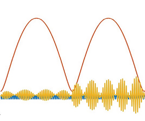
Provided the coefficient of $\tilde {T}^2$ here is positive, this is a fly away solution. Figure 4 shows that the solution from the full computation and the approximate parabolic curve from (4.6) overlap very closely, which indicates firm agreement; $\theta (T)$ is also shown to be an oscillating function of time as predicted analytically.

Figure 4.

A fly away case. The numerical solutions of $h$ and $\theta$ for a body with $M = 1, I=0.2$, $F_u(X) = -0.2\sin {\rm \pi}X$ and incoming profile $u_0 = Y+1$ are shown in blue. Initial conditions are $h(0) = 1, \theta (0) = -0.2, h_T(0) = 0, \theta _T(0) = 0.$ Red shows the parabolic approximation given in (4.6) (it overlaps very closely with the blue curve).

4.1. The $\theta _0$ limit cycle

Of natural interest is the question of how (or if) one can tell if fly away will occur without running full simulations. In light of (4.6), it is clear that to do this requires an understanding of the $\theta _0$ limit cycle and its mean and variance. Equation (4.4) can be integrated to obtain

(4.7)\begin{equation} I\left(\frac{{\rm d}\theta_0}{{\rm d}T}\right)^2 = 2c_0\theta_0+c_1\theta_0^2+\frac{2}{3}c_2\theta_0^3 + k, \end{equation}

for some constant $k$, which is related to $\langle \theta _0\rangle$ by

(4.8)\begin{equation} \langle\theta_0\rangle = \frac{1}{T_0}\int_T^{T+T_0} \theta_0\, {\rm d}T = \frac{2\sqrt{I}}{T_0}\int_{\theta_{{min}}}^{\theta_{{max}}} \frac{u}{\sqrt{2c_0u+c_1u^2+\tfrac{2}{3}c_2u^3+k}}\, {\rm d}u, \end{equation}

where the minimum $\theta _{{min}}$ and the maximum $\theta _{{max}}$ of $\theta _0$ are functions of $k$ in the sense that they are the two real solutions to the equation $0= 2c_0\theta _0+c_1\theta _0^2+\frac {2}{3}c_2\theta _0^3 + k.$ Similarly, the period $T_0$ is given by

(4.9)\begin{equation} T_0 = \int_T^{T+T_0}\,{\rm d}T = 2\sqrt{I}\int_{\theta_{{min}}}^{\theta_{{max}}}\frac{1}{\sqrt{2c_0u+c_1u^2+\tfrac{2}{3}c_2u^3+k}}\, {\rm d}u. \end{equation}

It is not easy to determine the value of $k$ as it depends on the behaviour of the system prior to entry into the ‘large $h$’ regime. However, $k$ can be easily bounded to force the cubic in (4.7) to have two real roots (else a limit cycle cannot exist), which in turn can produce a range of viable $\langle \theta _0\rangle$ values. Because $\langle \theta _{0TT}\rangle = 0$, we have

(4.10)\begin{equation} \langle\theta_0^2\rangle ={-}\frac{1}{c_2}\left(c_0+c_1\langle\theta_0\rangle\right), \end{equation}

which can be used to bound the parabola coefficient. Thus, although we cannot determine the exact behaviour of the body for given initial conditions without running full simulations, we will know the range of possible values of the parabola coefficient which gives a range of possible behaviours, e.g. if the range is entirely positive, then fly away is guaranteed following lift-off, and if not, there may exist some other types of solution such as those discussed in §§ 5 and 6 below.

5. ‘Bouncing’ solutions

Numerical results reveal the existence of solutions for which $h$ ‘bounces’, i.e. reaches large values then comes back to $O(1)$ repeatedly. We will show cases where $H_2 \equiv 0$, and hence $a_0+a_1\langle \theta _0\rangle +a_2\langle \theta _0^2\rangle = 0.$ To examine these, we need to take the analysis to the next order, so let $h = \tau H_1(\tilde {T})+H_0(T)$ and $\theta = \theta _0(T)+\tau ^{-1}\theta _{-1}(T).$ Proceeding as before, the body motion equations at the next order are

(5.1)$$\begin{gather} M\frac{{\rm d}^2H_1}{{\rm d}\tilde{T}^2} = \frac{k_1}{H_1}+a_1\langle\theta_{{-}1}\rangle+2a_2\langle\theta_0\theta_{{-}1}\rangle, \end{gather}$$

(5.2)$$\begin{gather}I\frac{{\rm d}^2\theta_{{-}1}}{{\rm d}T^2} = \frac{k_2(T)}{H_1}+ c_1\theta_{{-}1}+2c_2\theta_0\theta_{{-}1}, \end{gather}$$

where

(5.3)$$\begin{gather} k_1 ={-}\int_0^1 \left\langle\vphantom{\frac{A}{2}}\left(A\left[(1-X)\theta_0-F_u(X)\right]+B\right)\left[(1-X)\theta_0-F_u(X)\right]\right.\nonumber\\ \left.\times\left(\frac{A}{2}\left[(1-X)\theta_0-F_u(X)\right]+B\right)\right\rangle\, {\rm d}X, \end{gather}$$

and

(5.4)$$\begin{gather} k_2(T)={-}\int_0^1 \left(A\left[(1-X)\theta_0-F_u(X)\right]+B\right)\left[(1-X)\theta_0-F_u(X)\right]\nonumber\\ \times\left(\frac{A}{2}\left[(1-X)\theta_0-F_u(X)\right]+B\right)(X-\beta)\, {\rm d}X, \end{gather}$$

define $k_1, k_2$ as the coefficients above.

5.1. Analysis for small $k_1$, $k_2$

We will assume that $k_1$ and $k_2$ are small: this is partly to make progress and partly because this has tended to be the case numerically. The possibility that $k_{1,2}$ are not small will be addressed at the end of the subsection. Then, for $H_1 = O(1),$ we have the system

(5.5)$$\begin{gather} M\frac{{\rm d}^2H_1}{{\rm d}\tilde{T}^2} = a_1\langle\theta_{{-}1}\rangle+2a_2\langle\theta_0\theta_{{-}1}\rangle, \end{gather}$$

(5.6)$$\begin{gather}I\frac{{\rm d}^2\theta_{{-}1}}{{\rm d}T^2} = c_1\theta_{{-}1}+2c_2\theta_0\theta_1. \end{gather}$$

Similarly to the previous solution, $\theta _{-1}$ is a periodic function and $\langle \theta _{-1}\rangle$ is a constant, which indicates that $H_1$ is parabolic to leading order. If the right-hand side of (5.5) is positive, then this describes the solution for all time, and we see a weaker but similar fly away solution. If it is negative, however, then $H_1 \to 0$ at some time $\tilde {T} = \tilde {T}_1$, and there is a second solution when $H_1$ is small. In this case, we rescale for small $H_1$ by letting $H_1 = k_1^{3/2}y$, $\theta _{-1} = k_1^{-1/2}\varTheta$ and $\tilde {T} = \tilde {T}_1+k_1t$ to find the new system

(5.7)$$\begin{gather} M\frac{{\rm d}^2y}{{\rm d}t^2} = \frac{1}{y}+k_1^{1/2}C(t), \end{gather}$$

(5.8)$$\begin{gather}I\frac{{\rm d}^2\varTheta}{{\rm d}T^2} = \frac{k_2(T)}{k_1}\frac{1}{y}+c_1\varTheta+2c_2\theta_0\varTheta, \end{gather}$$

where we have also defined $C$ as the right-hand side of (5.5) for convenience ($C = C(t)$ is not a constant in this boundary layer solution). The expansion $y = y_0+k_1^{1/2}y_1+\cdots$ yields

(5.9)$$\begin{gather} M\frac{{\rm d}^2y_0}{{\rm d}t^2} = \frac{1}{y_0}, \end{gather}$$

(5.10)$$\begin{gather}M\frac{{\rm d}^2y_1}{{\rm d}t^2} ={-}\frac{y_1}{y_0^2} + C(t). \end{gather}$$

The solution to (5.9) is

(5.11)\begin{equation} y_0 = y_{0\,min}\exp\left(\left[\mathrm{erfi}^{{-}1}\left(\sqrt{\frac{2}{{\rm \pi} M}}\frac{t}{y_{0\,min}}\right)\right]^2\right), \end{equation}

where $\mathrm {erfi}^{-1}$ is the inverse of the imaginary error function. We can understand its behaviour by integrating and considering its phase portrait,

(5.12)\begin{equation} \frac{M}{2}\left(\frac{{\rm d}y_0}{{\rm d}t}\right)^2 = \log |y_0| + \text{const.} \end{equation}

Here, starting from $t = -\infty$, $y_0$ decreases from $\infty$ close to linearly (like $t(\log t)^{1/2}$), passes through a minimum point at $(0,y_{0\,min})$, then leaves symmetrically to $+\infty$, so that $y_0$ and hence $H_1$ apparently ‘bounces’. Numerical results from full simulations (shown in figure 5) confirm this behaviour, and simulations of the reduced system (5.7) and (5.8) in figure 6 show that the effect of the bounce is ultimately to push $\theta _{-1}$ into a different limit cycle, so that in the next excursion, although $C$ is again constant, it takes a new value. This produces repeated excursions of varying height and length, as observed numerically.

Figure 5.

A bouncing case. The numerical solutions of $h$ and $\theta$ for a body with $M = 1, I=0.2$, $F_u(X) = -0.2\sin {\rm \pi}X$ and incoming profile $u_0 = 3.2Y+1$ are shown in blue. Initial conditions are $h(0) = 1, \theta (0) = -0.2, h_T(0) = 0, \theta _T(0) = 0.$

Figure 6.

Bouncing. The results of a simulation for which $\theta _0$ is calculated using (4.4), and $h$ and $\theta _{-1}$ are calculated using (5.5) and (5.6). Values for $k_{1,2}$ and $C$ as well as initial conditions for $\theta _0$ are taken as constants from full simulations. Because $C$ is taken as constant, we see $h$ repeats the same excursion – but in reality, the shift in the $\theta _{-1}$ limit cycle would produce distinct excursions as shown in the full results of figure 5.

The ‘bouncing’ behaviour here should be observed regardless of the sizes of $k_1, k_2$, provided they are similar in size; if $k_{1,2}/H_1$ is small, we see $\theta _{-1}$ oscillating and $H_1$ decreasing parabolically, until $H_1$ becomes small enough that $k_1/H$ becomes the dominant term in (5.5), causing the body to ‘bounce’ and re-enter the parabolic regime.

6. Other behaviour

The findings above point to further behaviours being possible in the current fluid/body interactions. These behaviours are associated with interactions in which the scaled body height $h$ oscillates as discussed below in § 6.1, or an alternative crash effect occurs which is described in § 6.2 or the scaled angle $\theta$ ceases to remain bounded as investigated in § 6.3 below.

6.1. Oscillating $h$ solutions

These are solutions for which $H_2 \equiv H_1 \equiv 0$. In this case, $h = H_0(T)$ and $\theta = \theta _0(T)$ are both periodic functions to leading order and $h$ never becomes large nor crashes. This is shown in figure 7. Because for these solutions $h$ and $\theta$ are of comparable size, analysis is difficult and less fruitful.

Figure 7.

An ‘oscillating $h$’ solution. The numerical solutions of $h$ and $\theta$ for a body with $M = 1, I=0.2$, $F_u(X) = -0.2\sin {\rm \pi}X$ and incoming profile $u_0 = 4Y+1$ are shown in blue. Initial conditions are $h(0) = 1, \theta (0) = -0.2, h_T(0) = 0, \theta _T(0) = 0.$

6.2. Parabolic crash

If $h$ is large in the initial conditions, strong negative parabolas can be realised. The body then crashes with $\langle h\rangle$ approximately linear, and $h, \theta$ oscillating. This is shown in figure 8. On smaller scales such that the effect of $H_0$ is visible, the 4/5 behaviour of § 3 is still shown, but on large scales, it cannot be seen in comparison to the large linear term in $h$.

Figure 8.

An ‘alternative crash’. The numerical solutions of $h$ and $\theta$ for a body with $M = 1, I=0.2$, $F_u(X) = -0.2\sin {\rm \pi}X$ and incoming profile $u_0 = 5Y+1$ are shown in blue. Initial conditions are $h(0) = 100, \theta (0) = -0.2, h_T(0) = 0, \theta _T(0) = 0.$

6.3. The $\theta$ escape solutions

Using (4.4) to examine the phase portrait for $\theta _0$, it is clear that there should also exist some ‘escape’ solutions, in which $\theta _0 \to \infty$. These can be realised if starting with large $h$. This also eventually causes a crash as the body turns on its side, but it might be physically questionable as large values of $\theta$ are not necessarily compatible with the small angle approximation that is used in the definition of the body curve. A numerical simulation of this case is shown in figure 9.

Figure 9.

A ‘$\theta$-escape’ solution. The numerical solutions of $h$ and $\theta$ for a body with $M = 1, I=0.2$, $F_u(X) = -0.2\sin {\rm \pi}X$ and incoming profile $u_0 = Y+1$ are shown in blue. Initial conditions are $h(0) = 100, \theta (0) = 0.2, h_T(0) = 0, \theta _T(0) = 0.$