1. Introduction
In a payment for environmental services (PES) program, the beneficiaries of environmental services must contribute monetarily to make the necessary investments for a conservation program. This money is used to compensate for the pecuniary losses of individuals who must abandon certain economic activities and/or change their production processes to protect the environment (Sierra and Russman, Reference Sierra and Russman2006; Pagiola, Reference Pagiola2008; Wunder et al., Reference Wunder, Engel and Pagiola2008; Wünscher et al., Reference Wünscher, Engel and Wunder2008; Van Hecken et al., Reference Van Hecken, Bastiaensen and Vásquez2012).
Demand analysis of environmental services has been identified as an important component in evaluating the feasibility of PES schemes (Southgate and Wunder, Reference Southgate and Wunder2007; Ortega-Pacheco et al., Reference Ortega-Pacheco, Lupi and Kaplowitz2009; Whittington and Pagiola, Reference Whittington and Pagiola2012). The demand is expressed as a population's willingness to pay (WTP) for certain environmental goods; it is generally estimated using stated preference techniques such as contingent valuation (CV) and choice experiments. Nevertheless, WTP estimations using the CV method in many real PES experiences have proved disappointing because few studies have satisfied the minimum number of quality indicators, such as using methods to reduce hypothetical bias, asking uncertainty questions and using visual aids to explain scenarios (Whittington and Pagiola, Reference Whittington and Pagiola2012).
Furthermore, Kosoy et al. (Reference Kosoy, Martinez-Tuna, Muradian and Martinez-Alier2007) and Whittington and Pagiola (Reference Whittington and Pagiola2012) showed that, in several PES experiences, the estimated mean WTPs for the programs were significantly higher than the final payment. This finding led Kosoy et al. (Reference Kosoy, Martinez-Tuna, Muradian and Martinez-Alier2007) to conclude that the technical studies did not influence the final design of the PES program and that WTP estimations overestimated the politically and socially feasible fees (Kosoy et al., Reference Kosoy, Martinez-Tuna, Muradian and Martinez-Alier2007: 454).
We believe that this disparity between the estimated WTP and the final payment in real implementations of PES can be avoided if researchers focus on other quantiles of WTP distribution. Generally, researchers who conduct CV studies focus on the mean or median of the WTP distribution (Carson and Hanemann, Reference Carson and Hanemann2005) because both welfare measures are appropriate in the context of damage assessments and cost-benefit analysis, such as the Exxon Valdez Oil Spill (Carson et al., Reference Carson, Mitchell, Hanemann, Kopp, Presser and Ruud2003). However, other quantiles of the distribution are relevant in PES applications.
Hanemann (Reference Hanemann1984) showed the relationship between the responses to a referendum CV study and the random utility theory (RUM) suggested by Lancaster (Reference Lancaster1966). In addition, the researcher depicted what is currently considered the classic means to obtain welfare measures from changes in environmental quality, which are summarized using measures of central tendency, such as the mean and median of the WTP. The selection between the mean and median has significant social and political implications because it has consequences for the aggregation of benefits in the population. The mean is consistent with the Kaldor–Hicks criterion of compensation, whereas the median is consistent with a majority criterion (Carson and Hanemann, Reference Carson and Hanemann2005). The median can be interpreted as the probability that a person is willing to pay that amount of money equal to 0.5; that is, the individual is at an indifference point between paying and not paying for the good. Extending this result to the population, 50 per cent of the population would be willing to pay this amount of money.
There is an important distinction between CV-PES applications and traditional CV studies. In contrast to traditional studies that focus on cost-benefit analysis, CV-PES studies attempt to identify whether the amount of money that could be collected with the PES scheme would be sufficient to support the project. In this context, sufficient support implies social and political feasibility and the collection of sufficient money to finance the project. Both Carson and Hanemann (Reference Carson and Hanemann2005: 862) and Whittington and Pagiola (Reference Whittington and Pagiola2012) argued that lower quantiles correspond to a supermajority voting; that is, lower quantiles of the WTP distribution imply higher political and social feasibility. We believe that policy makers would be more inclined to support projects that do not have significant social opposition, that is, those projects that a supermajority would be willing to support. As Whittington and Pagiola (Reference Whittington and Pagiola2012) noted, in a PES context, using the mean of the WTP may leave a significant number of people paying more than they are willing to and thus may generate a high level of public opposition to the project due to a significant welfare loss for those households.
Although Carson and Hanemann (Reference Carson and Hanemann2005) and Whittington and Pagiola (Reference Whittington and Pagiola2012) explicitly discussed the possibility of deriving other percentiles of the estimated WTP distribution, to the best of our knowledge there are two applications of quantile regression to CV (Belluzzo, Reference Belluzzo2004; O'Garra and Mourato, Reference O'Garra and Mourato2006). O'Garra and Mourato (Reference O'Garra and Mourato2006) used a payment card as an elicitation format; therefore, their dependent variable is continuous (truncated at zero). The researchers use a classical (frequentist) continuous quantile regression for their WTP estimation (Tobit model). In contrast, our application uses a discrete choice model and a Bayesian estimation.
The closest paper to our application is Belluzzo (Reference Belluzzo2004), who estimated the quantiles of welfare measures using a discrete choice model inspired by the theoretical approach suggested by Cameron (Reference Cameron1988) and a frequentist estimation method. The researcher used the Smoothed Maximum Score estimator (Manski, Reference Manski1975, Reference Manski1985; Horowitz, Reference Horowitz1992; Kordas, Reference Kordas2006), which contains difficulties in its estimation and inference (Delgado et al., Reference Delgado, Rodríguez-Poo and Wolf2001; Abrevaya and Huang, Reference Abrevaya and Huang2005; Florios and Skouras, Reference Florios and Skouras2008).
In summary, our paper is the first application of a Bayesian quantile regression to CV using the indirect utility approach Hanemann (Reference Hanemann1984). Our application used data from a CV-PES application with the objective of conserving the hydrological ecosystem services (HES) provided by forest in the upper and middle Piraí River basin (including the Amboró National Park) in the Department of Santa Cruz, Bolivia.
Quantile regression allows the estimated coefficients to change over quantiles and, therefore, allows us to understand whether the explanatory variable exerts different impacts on different parts for the WTP distribution. This question cannot be evaluated with the conventional RUM approach. Bayesian estimation does not have the same estimation problems that are pervasive in frequentist binary quantile regression (Benoit and Van den Poel, Reference Benoit and Van den Poel2012). This estimation also provides the entire distribution of the parameters of interest, not simply a point estimate; this leads to inference conditional on the observed data as opposed to the asymptotic inference of the classical approach, and better addresses parameter uncertainty (Yu et al., Reference Yu, Lu and Stander2003).
The following section describes the research methods, including CV and its relationship with PES, the estimation methods and the calculation of the WTP. Section 3 describes the PES program under analysis in Bolivia. Section 4 describes the main results of the WTP estimations. Finally, section 5 discusses the relevance of our CV results and presents our conclusions.
2. Research methods
2.1. The contingent valuation method and payment for environmental services
CV uses questionnaires to elicit people's WTP for a good or service, creating a hypothetical market in which people can declare their preferences for the good. There have been over a thousand applications of CV studies in diverse areas of economics; the main results are summarized in a number of books covering theoretical and empirical issues (Mitchell and Carson, Reference Mitchell and Carson1989; Bateman et al., Reference Bateman, Willis and Arrow2001; Champ et al., Reference Champ, Boyle and Brown2003). Additionally, certain guidelines on best CV practices can be found in Arrow and Solow (Reference Arrow and Solow1993) and in Whittington and Pagiola (Reference Whittington and Pagiola2012). Among these practices, the suggested elicitation method is the closed-ended format for the WTP question in which respondents encounter a randomly assigned amount of money $A as a price for the environmental service (ES), and they decide whether they are willing to pay this amount.
Despite the pervasive presence of CV studies in several areas of economics, their application has been highly controversial. A discussion of these controversies is beyond the scope of this paper; however, an appropriate starting point for the interested reader is presented in the Journal of Economic Perspective’s CV symposium (Carson, Reference Carson2012; Hausman, Reference Hausman2012).
In the context of a PES, CV is used to estimate the maximum amount of money that the beneficiaries of a project are willing to pay to implement a program that ensures the provision of an ES. Certain valuation studies of ES are those by Zhongmin et al. (Reference Zhongmin, Guodong, Zhiqiang, Zhiyong and Loomis2003), Jin et al. (Reference Jin, Wang and Liu2008) and Loureiro and Ojea (Reference Loureiro and Ojea2008), and examples that deal specifically with PES include studies by Ortega-Pacheco et al. (Reference Ortega-Pacheco, Lupi and Kaplowitz2009), Van Hecken et al. (Reference Van Hecken, Bastiaensen and Vásquez2012) and Moreno-Sanchez et al. (Reference Moreno-Sanchez, Maldonado, Wunder and Borda-Almanza2012).
2.2. Estimating a binary quantile regression
Given that the elicitation question is the closed-ended format in which respondents encounter an amount of money $A as a price for the ES and they decide whether they are willing to pay this amount, we will solely have a positive (yes) or a negative (no) answer. We denote a positive answer of individual i as y
i
= 1 and a negative answer as y
i
= 0. As Haab and McConnell (Reference Haab and McConnell2002) described, a CV model assumes that the satisfaction that a consumer perceives can be represented by a utility function, denoted by u
j
, which has a deterministic component $v_{j}(p,I,q_{j})$
and a random component
$v_{j}(p,I,q_{j})$
and a random component $\varepsilon_{j}$
. That is,
$\varepsilon_{j}$
. That is, $u_{j} = v_{j}(p,I,q_{j})+ \varepsilon_{j}$
, where j = 0 denotes the initial situation, j = 1 denotes the new situation, p is a vector of current prices, I is income and q
j
represents the environmental quality (we have dropped the individual's subscript i). A respondent will be willing to pay the amount A only if the utility of paying for this project is higher than the utility of the status quo in which he or she does not pay for the project (Hanemann and Kanninen, Reference Hanemann, Kanninen, Bateman and Willis1999) (u
1>u
0). Therefore, the probability of a positive (yes) answer is:
$u_{j} = v_{j}(p,I,q_{j})+ \varepsilon_{j}$
, where j = 0 denotes the initial situation, j = 1 denotes the new situation, p is a vector of current prices, I is income and q
j
represents the environmental quality (we have dropped the individual's subscript i). A respondent will be willing to pay the amount A only if the utility of paying for this project is higher than the utility of the status quo in which he or she does not pay for the project (Hanemann and Kanninen, Reference Hanemann, Kanninen, Bateman and Willis1999) (u
1>u
0). Therefore, the probability of a positive (yes) answer is:
 $$Pr (yes) = Pr [\Delta v \gt \eta] = F_{\eta} (\Delta v)$$
with $\Delta v = v_{1}(p,I - A,q_{1}) - v_0 (p,I,q_0), \eta = \varepsilon_0 - \varepsilon_1$
and F
η as the distribution function of η.
$\Delta v = v_{1}(p,I - A,q_{1}) - v_0 (p,I,q_0), \eta = \varepsilon_0 - \varepsilon_1$
and F
η as the distribution function of η.
We used a Bayesian approach based on an asymmetric Laplace distribution (ALD) to estimate a binary quantile regression using a parametric linear utility function given by $v_{j}=\alpha_{j}+\beta I + \varepsilon_{j}$
(for other functional forms, refer to Hanemann, Reference Hanemann1984). It can be shown that for this utility function Δv = α−βA, β>0, α = (α1−α0). Other explanatory variables enter into the model through coefficient α. The linear utility function is the most popular functional form used in the stated preference models due to the simplicity of estimating both the random utility model and WTP (Louviere et al., Reference Louviere, Hensher and Swait2000). The Bayesian approach used in this paper does not have convergence problems; it is simple to estimate, valid for small sample sizes, robust to heteroskedasticity and guarantees a global optimum in comparison to classic approaches, such as the Maximum Score (Manski, Reference Manski1985) and the Smoothed Maximum Score (Kordas, Reference Kordas2006; Florios and Skouras, Reference Florios and Skouras2008). Furthermore, the estimators are consistent, efficient, asymptotically normal and admissible (Cameron and Trivedi, Reference Cameron and Trivedi2005; Rossi and McCulloch, Reference Rossi and McCulloch2010).
$v_{j}=\alpha_{j}+\beta I + \varepsilon_{j}$
(for other functional forms, refer to Hanemann, Reference Hanemann1984). It can be shown that for this utility function Δv = α−βA, β>0, α = (α1−α0). Other explanatory variables enter into the model through coefficient α. The linear utility function is the most popular functional form used in the stated preference models due to the simplicity of estimating both the random utility model and WTP (Louviere et al., Reference Louviere, Hensher and Swait2000). The Bayesian approach used in this paper does not have convergence problems; it is simple to estimate, valid for small sample sizes, robust to heteroskedasticity and guarantees a global optimum in comparison to classic approaches, such as the Maximum Score (Manski, Reference Manski1985) and the Smoothed Maximum Score (Kordas, Reference Kordas2006; Florios and Skouras, Reference Florios and Skouras2008). Furthermore, the estimators are consistent, efficient, asymptotically normal and admissible (Cameron and Trivedi, Reference Cameron and Trivedi2005; Rossi and McCulloch, Reference Rossi and McCulloch2010).
As Hanemann (Reference Hanemann1984) noted, one needs an assumption regarding the distribution of the difference in the error terms of two indirect utility functions $(\eta = \varepsilon_{1} - \varepsilon_0)$
. In the conventional RUM approach, it is assumed that η has either a logistic or a normal distribution. For the Bayesian estimation, it is convenient to assume that η has an ALD (Hewson and Yu, Reference Hewson and Yu2008; Benoit and Van den Poel, Reference Benoit and Van den Poel2012) because the likelihood function associated with the ALD is directly related to the minimization problem associated with a quantile regression. Consider that a quantile regression will solve the following problem (Benoit and Van den Poel, Reference Benoit and Van den Poel2012).
$(\eta = \varepsilon_{1} - \varepsilon_0)$
. In the conventional RUM approach, it is assumed that η has either a logistic or a normal distribution. For the Bayesian estimation, it is convenient to assume that η has an ALD (Hewson and Yu, Reference Hewson and Yu2008; Benoit and Van den Poel, Reference Benoit and Van den Poel2012) because the likelihood function associated with the ALD is directly related to the minimization problem associated with a quantile regression. Consider that a quantile regression will solve the following problem (Benoit and Van den Poel, Reference Benoit and Van den Poel2012).
 $$\tilde{\beta} = \arg \min \sum\limits_{i=1}^N \rho_{\tau} (y_i - x_i^{\prime} \beta),$$
in which $\rho_{\tau} (z) = z \lpar \tau -I(z \lt 0) \rpar $
, I(z<0) is an indicator function and τ∈(0, 1). This function assigns the weight τ to positive values of z and (1−τ) to negative values of z. Furthermore, a random variable y
i
with ALD has a density function given by
$\rho_{\tau} (z) = z \lpar \tau -I(z \lt 0) \rpar $
, I(z<0) is an indicator function and τ∈(0, 1). This function assigns the weight τ to positive values of z and (1−τ) to negative values of z. Furthermore, a random variable y
i
with ALD has a density function given by
 $$f(y\vert \theta,\sigma, \tau)= {\tau (1 - \tau) \over \sigma} \exp \left(-\rho_{\tau} \left({y - \theta \over \sigma} \right) \right),$$
in which τ is the asymmetry coefficient, $-\infty \lt \theta \lt \infty $
(we could define
$-\infty \lt \theta \lt \infty $
(we could define $\theta =x_{i}^{\prime} \beta $
) is the location parameter, and σ>0 is the scale parameter. The main argument of this distribution (Yu and Zhang, Reference Yu and Zhang2005) is the same argument as equation (2).
$\theta =x_{i}^{\prime} \beta $
) is the location parameter, and σ>0 is the scale parameter. The main argument of this distribution (Yu and Zhang, Reference Yu and Zhang2005) is the same argument as equation (2).
Assuming that η has an ALD is convenient but not crucial. Li et al. (Reference Li, Xi and Lin2010) showed that the Bayesian quantile regression is robust to ‘functional form’ assumptions; in fact, many Monte Carlo simulations assume that the original error term is normally distributed (Li et al., Reference Li, Xi and Lin2010; Benoit and Van den Poel, Reference Benoit and Van den Poel2012) and use the likelihood function of a ALD for the estimation. As Yu and Moyeed (Reference Yu and Moyeed2001) noted, it is not necessary to specify the distribution of the error term.
The Bayesian approach relies on a combination of a prior distribution for the coefficients and the likelihood function, which provides a posterior distribution for the coefficients. In accordance with Benoit and Van den Poel (Reference Benoit and Van den Poel2012), if we assume that the difference in an indirect utility function $\Delta v^{\ast} $
is a linear function of the error term η, which is distributed as a Laplace distribution, that is,
$\Delta v^{\ast} $
is a linear function of the error term η, which is distributed as a Laplace distribution, that is, $\eta \sim {ALD}({0,1,\tau}),$
then the latent variables
$\eta \sim {ALD}({0,1,\tau}),$
then the latent variables $\Delta v^{\ast} $
have an ALD of the form
$\Delta v^{\ast} $
have an ALD of the form $\Delta v^{\ast} \sim {ALD}({\theta = x_{i}^{T} \beta,\sigma =1,\tau})$
, where
$\Delta v^{\ast} \sim {ALD}({\theta = x_{i}^{T} \beta,\sigma =1,\tau})$
, where $\theta_{\tau} =x_{i}^{T} \beta =\alpha_{\tau} -\beta_{\tau} A_{t} $
is the location parameter and σ is the scale parameter. The τ parameter should be specified at the quantile of interest, with τ∈(0, 1).
$\theta_{\tau} =x_{i}^{T} \beta =\alpha_{\tau} -\beta_{\tau} A_{t} $
is the location parameter and σ is the scale parameter. The τ parameter should be specified at the quantile of interest, with τ∈(0, 1).
Given that in a binary CV people's responses are codified as y
i
= 1 for a positive response, that is $\Delta v_{i}^{\ast} \gt 0$
, and y
i
= 0 in other cases (
$\Delta v_{i}^{\ast} \gt 0$
, and y
i
= 0 in other cases ( $\Delta v_{i}^{\ast} \lt 0$
), then,
$\Delta v_{i}^{\ast} \lt 0$
), then,
 $$P\lpar y_i = 1 \rpar = 1 - F_{y_i^{\ast}} \lpar - x_i^{\prime} \beta \rpar ,$$
where $F_{y_{i}^{\ast}} (.)$
is the cumulative distribution function of the asymmetric Laplace latent variable
$F_{y_{i}^{\ast}} (.)$
is the cumulative distribution function of the asymmetric Laplace latent variable $\Delta v_{i}^{\ast} $
. Therefore, the joint posterior density for β and
$\Delta v_{i}^{\ast} $
. Therefore, the joint posterior density for β and $\Delta v_{i}^{\ast} $
, given people's responses, is
$\Delta v_{i}^{\ast} $
, given people's responses, is $y = (y_{1},\ldots,y_{n})$
and the quantile τ is:
$y = (y_{1},\ldots,y_{n})$
and the quantile τ is:
 $$\eqalign{&\pi ({\beta,\Delta v^\ast \vert y,x,\tau})\propto \pi (\beta)\prod_{i=1}^n \{ {I({\Delta v_i^{\ast} \gt 0})I({y_i =1})+I({\Delta v_i^{\ast} \le 0})\,I({y_i =0})} \}\cr &\quad \times F_{y_i^{\ast}} ({\Delta v_i^{\ast}; x_i^{\prime} \beta, 1, \tau}),}$$
where I(.) is an indicator function, and π (β) is a prior distribution. As in Benoit and Van den Poel (Reference Benoit and Van den Poel2012), we assume that the prior of the π (β) parameters follows a normal distribution; that is, $\pi(\beta)\sim N(\bar{\beta}_{0}, V_{0})$
, where
$\pi(\beta)\sim N(\bar{\beta}_{0}, V_{0})$
, where $\bar{\beta}_{0}$
is the vector of means of the k×1 order prior and V
0 is the matrix of variances and covariance of β of k×k order.
$\bar{\beta}_{0}$
is the vector of means of the k×1 order prior and V
0 is the matrix of variances and covariance of β of k×k order.
Although we cannot sample from this unknown posterior distribution, we could use a MCMC algorithm. Benoit and Van den Poel (Reference Benoit and Van den Poel2012) suggested a Metropolis–Hasting within Gibbs algorithm that splits the posterior distribution into a conditional distribution of β given $\Delta v^{\ast}$
and a distribution of
$\Delta v^{\ast}$
and a distribution of $\Delta v^{\ast}$
given β. They also show that the conditional distribution of
$\Delta v^{\ast}$
given β. They also show that the conditional distribution of $\Delta v^{\ast}$
given is a three-parameter ALD truncated from the left at zero when y = 1 and a three-parameter ALD truncated from the right at zero if y = 0; that is,
$\Delta v^{\ast}$
given is a three-parameter ALD truncated from the left at zero when y = 1 and a three-parameter ALD truncated from the right at zero if y = 0; that is, $\pi (\Delta v^{\ast} \vert \beta, y, \tau)$
. Furthermore, this distribution is known, and one can sample from this distribution in a similar manner to sampling from a normal distribution.Footnote
1
$\pi (\Delta v^{\ast} \vert \beta, y, \tau)$
. Furthermore, this distribution is known, and one can sample from this distribution in a similar manner to sampling from a normal distribution.Footnote
1
To complete the simulation, we need the conditional posterior distribution of β given $\Delta v^{\ast}$
represented by
$\Delta v^{\ast}$
represented by
 $$\pi \lpar {\beta,\vert \Delta v^\ast,y,\tau} \rpar \propto \pi \lpar \beta \rpar \mathop \prod \limits_{i=1}^n \,F_{y_i^{\ast}} \lpar \Delta v_i^{\ast}; \,x_i^{\prime} \beta, 1, \tau \rpar .$$
The joint posterior function is generated from a block of conditional equations between $\Delta v^{\ast}$
and β; that is, given the data, the prior distribution and the quantile of interest, the join posterior distribution is obtained by sequentially drawing values from the truncated
$\Delta v^{\ast}$
and β; that is, given the data, the prior distribution and the quantile of interest, the join posterior distribution is obtained by sequentially drawing values from the truncated $\hbox{ALD}(x_{i}^{\prime} \beta,1,\tau)$
that characterizes
$\hbox{ALD}(x_{i}^{\prime} \beta,1,\tau)$
that characterizes $\pi \lpar \Delta v^{\ast} \vert \beta,y,\tau \rpar $
and the conditional posterior distribution
$\pi \lpar \Delta v^{\ast} \vert \beta,y,\tau \rpar $
and the conditional posterior distribution $\pi \lpar \beta, \vert \Delta v^{\ast}, y, \tau \rpar $
. Benoit and Van den Poel (Reference Benoit and Van den Poel2012) incorporated this Gibbs sampler to the bayesQR statistical package of the R program.
$\pi \lpar \beta, \vert \Delta v^{\ast}, y, \tau \rpar $
. Benoit and Van den Poel (Reference Benoit and Van den Poel2012) incorporated this Gibbs sampler to the bayesQR statistical package of the R program.
2.3. Estimating the willingness to pay
After estimating a linear functional form, we can obtain the mean (and median) of the WTP distribution (known as compensation variation and denoted generally by C) as $\hbox{C} = \hbox{E(WTP)} = \alpha /\beta$
(Haab and McConnell, Reference Haab and McConnell2002). However, our purpose is to estimate the mean at each quantiles regression; therefore, we add a subscript τ, C
τ, to denote the corresponding quantile and, using the same logic suggested by Hanemann (Reference Hanemann1984), we estimate the mean as:
$\hbox{C} = \hbox{E(WTP)} = \alpha /\beta$
(Haab and McConnell, Reference Haab and McConnell2002). However, our purpose is to estimate the mean at each quantiles regression; therefore, we add a subscript τ, C
τ, to denote the corresponding quantile and, using the same logic suggested by Hanemann (Reference Hanemann1984), we estimate the mean as:
 $$C_{\tau}^{+} = {\alpha_\tau \over \beta_\tau}.$$
Notice that we can estimate the ‘median’ or other percentiles of the distribution of each quantile regression using:
 $$\eqalign{F_\eta [\Delta v_{\tau} (C_\tau^{\ast})] &= F_\eta [\alpha_\tau - \beta_{\tau} C_\tau^{\ast}] = p, \quad \hbox{where} p\in (0,1). \cr F_\eta^{-1} [p] &= \alpha_\tau - \beta_{\tau} C_{\tau}^{\ast}, \cr C_\tau^{\ast} &= {\alpha_{\tau} - F_{\eta}^{-1} [p] \over \beta_{\tau}}.}$$
p is simply the probability that a person would be willing to pay the amount A in that portion of distribution of the dependent variable. In this case, F
η is the cumulative density function of ALD, ατ and βτ are the estimated parameters, and $C_{\tau}^{\ast}$
is the quantile welfare measure that satisfies the equality in equation (4). Furthermore,
$C_{\tau}^{\ast}$
is the quantile welfare measure that satisfies the equality in equation (4). Furthermore, $F_{\eta}^{-1}[p]$
is the inverse ALD with
$F_{\eta}^{-1}[p]$
is the inverse ALD with $F_{\eta}^{-1} [p=0.5]=0$
,
$F_{\eta}^{-1} [p=0.5]=0$
, $F_{\eta}^{-1} [p=0.6]=-0.455$
and
$F_{\eta}^{-1} [p=0.6]=-0.455$
and $F_{\eta}^{-1}[p=0.9] = -5.87$
.
$F_{\eta}^{-1}[p=0.9] = -5.87$
.
It is feasible to estimate the quantile of the distribution of the mean WTP provided by the conventional RUM logit (or probit) model, but this is analogous to estimating the predicted quantile in equation (4) for an arbitrary τ using the α and β instead of ατ and βτ. A main difference between our approach and a traditional RUM approach is that we estimate ατ and βτ for each τ, whereas a traditional approach only has one overall estimate for α and β. This approach allows us to have a better description of the distribution and the credible intervals at each quantile.
Whether they differ significantly is an empirical question, but even if they do not differ significantly the Bayesian quantile regression will provide a distribution of the WTP at each quantile, not only a point. Furthermore, the Bayesian quantile approach allows us to capture the heterogeneous effect of the explanatory variables across quantiles. For instance, individuals with a higher probability of accepting the payment may also be less affected by the increase in the BID.
3. Description and the payment for environmental services proposal
The sub-Andean forests of Bolivia are vital for the integrity of Bolivia's ecosystems. This region constitutes a large infiltration area for the lowland's groundwater (Ibisch et al., Reference Ibisch, Araujo and Nowicki2007), playing an important role in generating a safe water source for the city of Santa Cruz and hundreds of villages. The proposed PES program targets conservation of the HES provided by the forest in the upper and middle Piraí River basin, which includes part of the Amboró National Park (an area comprising 236,000 ha), which is located in the west of the Department of Santa Cruz.
Currently, these forests are under significant ecological pressure due to new settlements and the resulting economic activities that convert forested lands into cropland and pastureland. Land use changes, together with inappropriate agricultural practices, have diminished biodiversity in this area, reduced its primary productivity and weakened the ecosystem's regulatory capacities, all of which affect the provision of HES. Therefore, the suppliers of ES are the rural communities in the upper and middle basin of the Piraí River. Conversely, the city of Santa Cruz (the beneficiaries or buyers of the services) offers favorable conditions for the introduction of a PES scheme due to its location along the lower courses of the Piraí River.
The HES were assessed through hydrological and climate modeling analysis under different scenarios of land use change (Ovando, Reference Ovando2009; Seiler, Reference Seiler2009). The ecosystem services involved the filtering, retention and storage of water in aquifers, which then provide water to the city of Santa Cruz.
3.1. Survey design and implementation
Applying the CV survey includes determining the target population and the sample, designing the questionnaire, validating the survey, selecting and training interviewers and, finally, applying the final version of the survey. The relevant population for our survey included the 252,136 households in the urban area of the city of Santa Cruz that constitute the potential demand for the PES scheme. The sample was of 501 observations and has an error of 4.4 per cent. Our sample was concentrated in middle and lower income levels due to difficulties interviewing people in the high-level income bracket (see table A1 in the appendix). We used a probabilistic polietapic sampling on two levels. First, we randomly selected the neighborhood and blocks, and then we systematically selected the households to be interviewed. This approach means that we selected one household on each block starting in the northern corner, and if we did not have an answer at that house, we skipped the next four houses and knocked on the door of the fifth house.
Empirical evidence has shown that the selection of the bid vector and the size of the subsamples in each value may affect the estimation of the mean WTP (Cooper, Reference Cooper1993). Therefore, we followed a sequential procedure to define the bid vector. We combined the minimization of the mean WTP variance with an observation of the empirical distribution of the WTP after a portion of the sample was collected. From pilot surveys of 100 observations, we obtained values for the WTP using an open-ended question; this information was used to define the bid vector and the size of the subsamples for each bid using the method suggested by Cooper (Reference Cooper1993).
3.1.1. Survey application
The design of the final survey followed three steps. First, we used three focus groups to explore people's reactions to specific aspects of the hypothetical scenario and to identify wording problems or misleading sections of the survey. Secondly, we applied two pilot surveys to test the instrument's design in the field. Thirdly, we applied the final version of the survey.Footnote 2
Three focus groups were conducted in November and December 2008. Each group was composed of eight participants, male and female heads of households aged 30–50 years old. Focus groups included people of low and medium socio-economic status, which comprise the majority of the population. The first group discussed people's levels of awareness regarding ES in general and their perceptions regarding the benefits they receive from the forests of the upper and middle Piraí River basin. We also captured the respondents’ reactions to the environmental problem described in the survey and the possible solutions they would recommend to solve this problem. The other two groups evaluated the entire CV scenario, including payment vehicles and visual aids. This evaluation allowed us to examine people's reactions to the proposal of a PES program and their WTP.
We applied two pilot surveys of 50 observations between January and March 2009. These two pilots were used to validate the questionnaire design and to find information regarding people's WTP using an open-ended format. We trained our interviewers in accordance with Whittington, (Reference Whittington2002). We explained the CV methodology's main issues, the survey's objective, the importance of maintaining neutrality throughout the survey and the scenario. Interviewers performed role-play interviews among team members closely supervised by our researchers. After each pilot survey, we held working meetings with all interviewers to identify problems and biases in the survey. The final survey was applied from April to June 2009, and 501 surveys were completed.
The final survey has three sections. First, we collected data regarding people's perceptions of the social and environmental problems in Santa Cruz, and this served as a warm-up section. The second section was devoted to the valuation study that included information explaining the environmental and economic problem as well as the possible PES scheme. In this section, we explained the study area, the water cycle and its relation to water availability in the city, and the stressors affecting the basin (we included pictures of logging and other activities). Additionally, we discussed the main environmental services provided by the basin, including water provision, and water flow regulation and its relation to floods, droughts, and climate.
We also explained the PES scheme, which consisted of a proposal to conserve forests in the upper and middle basin of the Piraí River by providing monetary compensation to landowners in the area to commit them to forest conservation. The program would include a contract between landowners and the PES agency and a monitoring system to verify that the landowners were fulfilling their commitments. Funding for this program would be collected from the population of the city of Santa Cruz (main beneficiaries) through an additional fee in their water bill. If this project were implemented, each household must pay an extra monthly amount to conserve the forests. Failure to obtain the support of the population implies that this project cannot be implemented, and deforestation in the middle and upper basin of the Piraí River will continue, which affects the water supply to the city of Santa Cruz (reducing quantity and quality).
The elicitation question was as follows: ‘Given this information, are you willing to pay monthly $ A Bolivians to support this project and in this way to preserve the forest in the upper and middle basin of the Piraí River and assure the provision of the environmental services including water provision, avoiding floods and droughts and maintaining favorable weather?’
To reduce hypothetical bias in our CV study, in addition to the NOAA Panel recommendations we applied the cheap talk script suggested by Cummings and Taylor (Reference Cummings and Taylor1999) and Martinsson and Carlsson (Reference Martinsson and Carlsson2006), and a reminder of the budget constraint of the respondents. The survey follows with debriefing questions to ascertain reasons for not paying, uncertainty regarding the response and the acceptance of the scenario.
Finally, the survey included a section that collected sociodemographic information, including water consumption, current water bills, age, income, size of the household, and education.
4. Results and discussion
We obtained 501 useful surveys with 236 negative answers. Of the 236 negative answers, the majority claimed economic reasons for not paying. These reasons included: ‘I cannot afford additional costs’ (23.7 per cent); ‘I'd rather spend that money on other goods’ or ‘The suggested cost is too high for my budget’ (30.2 per cent). Another large group believed that it was not their responsibility to pay for these services and claimed that the government should pay for them (22 per cent). The fourth main reason was lack of confidence that the money would be spent on the plan (15 per cent). Eleven people said that they did not believe that the program would have any benefit.
Our level of protests is standard in the literature, particularly in developing countries. For instance, Atkinson et al. (Reference Atkinson, Healey and Mourato2005) found that approximately 34 per cent were protesters, and they simply removed the protesters from the sample and calculated the statistics with the non-protesters. This strategy should not yield any effect on the mean WTP if the number of protests is low, the sample is relatively large or protesters are similar to non-protesters. Otherwise, simply eliminating these individuals would cause a selection bias, which could invalidate the estimations (Calia and Strazzera, Reference Calia and Strazzera2001).
We decided to assume that they were acceptable zeros for two reasons. First, our review of the literature suggests that the most conservative approach is to accept all protests as zero values (Halstead et al., Reference Halstead, Luloff and Stevens1992; Meyerhoff and Liebe, Reference Meyerhoff and Liebe2006, Reference Meyerhoff and Liebe2010; Meyerhoff et al., Reference Meyerhoff, Mørkbak and Olsen2013). Secondly, we are interested in a PES scheme where the reason why people are not willing to pay is less relevant than in a cost-benefit analysis. In other words, if the person does not believe that the money will be spent on the project, even if his/her value is positive, he will vote against the project.
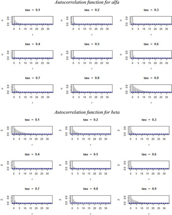
In Bayesian econometrics, we are concerned with the convergence of the MCMC for the parameters. We tested that our results were robust using the potential scale reduction factor (PSRF) proposed by Gelman and Rubin (Reference Gelman and Rubin1992). The results for different initial values of the parameters show a PSRF close to 1, which ensures the convergence of the MCMC. Additionally, we include in the appendix figure A1, which shows the autocorrelation plots for both the intercept and the bid coefficient. In general, we observe a rapid decline in the autocorrelation for all quantiles. For the extreme quantiles, we do observe slightly more correlation, which implies that it remains possible to improve the mixing.
Table 1 shows the estimated coefficient for several quantiles, including an intercept, the bid vector (BID), socio-economic status measure in five levels (NSE), AGE, Education (EDUC), and Household Size, and their credible interval (CI) at 95 per cent. The last column presents the estimated WTP. The BID should affect the WTP negatively according to demand theory (Hanemann, Reference Hanemann1984), while socio-economic status should have a positive sign on WTP since it indicates a higher ability to pay (Amponin et al., Reference Amponin, Bennagen, Hess and Dela Cruz2007). Education should also be correlated with ability to pay and therefore a positive sign is expected (Zhongmin et al., Reference Zhongmin, Guodong, Zhiqiang, Zhiyong and Loomis2003; Belluzzo, Reference Belluzzo2004); nevertheless, O'Garra and Mourato (Reference O'Garra and Mourato2006) found a negative effect for this variable in a quantile regression analysis. For age and household size, both the expected theoretical sign and the empirical evidence are ambiguous. It has been argued that older people care more about future generations or that they are more conscious about health issues, implying a positive impact of age on the WTP (Muhammad et al., Reference Muhammad, Fathelrahman and Ullah2015; Brouwer et al., Reference Brouwer, Brouwer, Eleveld, Verbraak, Wagtendonk and van der Woerd2016). Others argue that younger people are more conscious about environmental issues, implying a negative impact on the WTP (Boadu, Reference Boadu1992; Belluzzo, Reference Belluzzo2004; O'Garra and Mourato, Reference O'Garra and Mourato2006; Shultz and Soliz, Reference Shultz and Soliz2007; Alpízar and Madrigal, Reference Alpízar and Madrigal2016). Similarly, some authors suggest that the higher the household's size the lower the WTP, since there are more competitive uses for the family income (Boadu, Reference Boadu1992; Amponin et al., Reference Amponin, Bennagen, Hess and Dela Cruz2007). Nevertheless, others authors argue that the presence of children at home would increase the WTP (Shultz and Soliz, Reference Shultz and Soliz2007). The empirical evidence provides negative (García-Llorente et al., Reference García-Llorente, Martín-López, Nunes, González, Alcorlo and Montes2011; Alpízar and Madrigal, Reference Alpízar and Madrigal2016), positive (Muhammad et al., Reference Muhammad, Fathelrahman and Ullah2015) and sometimes insignificant results for this variable (Johnson and Baltodano, Reference Johnson and Baltodano2004; García-Llorente et al., Reference García-Llorente, Martín-López, Nunes, González, Alcorlo and Montes2011).
Table 1. Binary quantile regression estimates and WTP quantiles

Notes: Confidence interval of 95%, below parameters. The numbers of simulations are r = 20000, thinning = 10. b This is Bolivian currency. Each quantile represents Pr(c ≤ c 0).
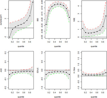
The intercept took negative values for quantiles 0.1 and 0.2 but was positive for the upper quantiles. All values for the bid vector were negative, which indicates a negative relation between the bid and the probability of paying. Higher socio-economic status and larger families are associated with a higher probability of paying the amount at all quantiles, whereas older people and those who are more educated are associated with a lower probability at all quantiles. Overall, considering all explanatory variables, there is a negative WTP in the two lowest quantiles, which is consistent with the literature on negative WTP (Haab and McConnell, Reference Haab and McConnell1997; Kriström, Reference Kriström1997); however, there is a positive WTP in the majority of the quantiles.
The interpretation of these quantiles’ WTP is the following: if we take the quantile 0.3, the mean WTP is equal to B$0.868 (US$0.08); that is, 70 per cent of the population is willing to pay at least 0.868 Bolivian, or 30 per cent of the population is not willing to pay this amount. Therefore, the data show that even at very low values of the environmental service fee, 30 per cent of the population would suffer a welfare loss or would not be willing to pay that amount of money. This finding is consistent with focus groups’ responses because they said they would be willing to pay B$10 (US$1.45) but that they considered that B$2 (US$0.291) would be a more reasonable value for the entire population. Notice that the mean is approximately B$21.3 (US$2.96), which is 37 times the value of the WTP at the quantile 0.3 and 10 times the value of what was suggested in the focus groups.
Figure 1 depicts the evolution of the coefficients of each explanatory variable by quantile. We observe that the BID coefficient changes among quantiles are larger in the lowest quantile and that it is not monotonic. The three coefficients that vary the most among quantiles are the intercept, the bid and the socio-economic level; the other three coefficients are different among quantiles but with less variance.

Figure 1. Coefficients for each explanatory variable for each quantile
We calculated the marginal WTP for each explanatory variable at each quantile as $MWTP = {\partial WTP^{q} \over \partial X} = {\beta_x^q \over \beta_{BID}^q}$
, where β
x
q
is the coefficient associated with the explanatory variable X and β
BID
q
is the coefficient associated with the variable BID in each quantile regression. We found an increasing and monotonic impact of socio-economic level and household size and a decreasing impact of AGE and EDU (considering only cases with a significant coefficient for β
x
q
). For instance, an increase in the socio-economic level will increase the WTP in 4.62, 4.74, 5.98, 7.5, 9.15, 10.4, 11.3, 12.9 and 14.9 Bolivians at each corresponding quantile. This is consistent with theoretical expectations; an explanatory variable should have a heterogeneous impact across quantiles. We expect a similar sign across quantiles but all explanatory variables will not necessarily be significant across quantiles because different drivers affect the WTP at different quantiles (Koenker, Reference Koenker2005; O'Garra and Mourato, Reference O'Garra and Mourato2006). To the best of our knowledge, the literature does not provide any discussion about the pattern associated with the impact of explanatory variables on WTP across quantiles. Koenker (Reference Koenker2005) shows that there is not a prior expectation about the behavior of coefficients across quantiles; in some cases they could vary randomly, while in others they could follow some pattern (increasing, decreasing). In our WTP model the definition of any expected pattern across quantiles is even more difficult since there are two parameters changing at the same time across quantiles (β
BID
q
, and β
x
q
); one of them is in the numerator and the other in the denominator of the WTP expression.
$MWTP = {\partial WTP^{q} \over \partial X} = {\beta_x^q \over \beta_{BID}^q}$
, where β
x
q
is the coefficient associated with the explanatory variable X and β
BID
q
is the coefficient associated with the variable BID in each quantile regression. We found an increasing and monotonic impact of socio-economic level and household size and a decreasing impact of AGE and EDU (considering only cases with a significant coefficient for β
x
q
). For instance, an increase in the socio-economic level will increase the WTP in 4.62, 4.74, 5.98, 7.5, 9.15, 10.4, 11.3, 12.9 and 14.9 Bolivians at each corresponding quantile. This is consistent with theoretical expectations; an explanatory variable should have a heterogeneous impact across quantiles. We expect a similar sign across quantiles but all explanatory variables will not necessarily be significant across quantiles because different drivers affect the WTP at different quantiles (Koenker, Reference Koenker2005; O'Garra and Mourato, Reference O'Garra and Mourato2006). To the best of our knowledge, the literature does not provide any discussion about the pattern associated with the impact of explanatory variables on WTP across quantiles. Koenker (Reference Koenker2005) shows that there is not a prior expectation about the behavior of coefficients across quantiles; in some cases they could vary randomly, while in others they could follow some pattern (increasing, decreasing). In our WTP model the definition of any expected pattern across quantiles is even more difficult since there are two parameters changing at the same time across quantiles (β
BID
q
, and β
x
q
); one of them is in the numerator and the other in the denominator of the WTP expression.
Considering these results, we could revisit the three examples provided by Kosoy et al. (Reference Kosoy, Martinez-Tuna, Muradian and Martinez-Alier2007) to observe whether lower quantiles of the distribution are closer to the final payment in the real applications of PES provided by these authors. These studies were located in Honduras, Nicaragua and Costa Rica; all of them have very small sample sizes for an acceptable discrete choice statistical analysis, which is considered the standard in applied CV literature. The authors provided no further information regarding the question's format (open-ended, closed-ended) or the econometric techniques used; therefore, our analysis is only speculative but is still illustrative of the benefit of the quantile analysis of WTP. The only information provided is that in Honduras the final payment was 3.6 per cent of the mean WTP, whereas in Costa Rica the final payment was 6 per cent of the standard water fee for households. For Nicaragua, no further details were provided regarding the difference; the researchers only noted that it differed considerably from the mean WTP. In our case, if we used B$0.868 as the new final charge for the PES, it would represent 2.68 per cent of the mean WTP, which is lower than the 3.6 per cent in Honduras. In addition, considering that respondents reported a mean of B$134 (US$19.39) for the standard water fee for households, our value would be 0.40 per cent of the average value, which is significantly lower than the value in Costa Rica. In contrast, if we considered the mean WTP, this value would be approximately 15 per cent of the standard water fee for households.
5. Conclusions
Our results show that the use of other quantiles framed in the supermajority concept (Whittington and Pagiola, Reference Whittington and Pagiola2012) provides a reasonable interpretation of the technical nonmarket valuation studies in the PES area. Using a CV application to value ecosystem services provided by the sub-Andean humid forest in the upper and middle Piraí River basin in Bolivia, our quantile regression analysis allowed us to estimate WTP values that are more informative in terms of the social and political feasibility of a PES scheme. Specifically, we found values that will be acceptable for a greater portion of the population, generating lower social and political opposition. Traditional applications of CV-PES use the mean of the distribution as a summary statistic of people's WTP; however, the political and social negotiation process resulted in a much lower final payment (Kosoy et al., Reference Kosoy, Martinez-Tuna, Muradian and Martinez-Alier2007). We found that the values of the mean WTP are 10–37 times higher than the value that would support a supermajority of 70 per cent of the population. The quantile analysis also allowed us to capture the heterogeneity among the population in terms of their WTP. This analysis may be useful to define different charges for different subgroups of the population, which is consistent with current water consumption subsidies in most urban areas.
For a PES scheme, the median (or mean for symmetric distributions) WTP may not be of significant interest because it is the value for which half the population is willing to pay. Therefore, assuring political and social support for the PES program may require a significantly higher proportion of people who are willing to pay a specific amount of money.
We completely agree with Kosoy et al. (Reference Kosoy, Martinez-Tuna, Muradian and Martinez-Alier2007) in that the final payment will be based on a complex social process with intricate interactions, which will finally depend on a negotiation among the parties and the underlying distance between the WTP and the WTA. Nevertheless, our results provide an additional means to take advantage of valuation studies to further inform the decision-making process. As Whittington and Pagiola (Reference Whittington and Pagiola2012) noted, CV-PES studies have been silent regarding the use of WTP estimates, which suggests the use of a public referendum with a supermajority. The quantile WTP estimation filled this gap.
Appendix

Figure A1. Coefficients for each explanatory variable for each quantile
Table A1. Socio-economic levels in Bolivia and the sample

Table A2. Descriptive statistics in the sample