


1. Introduction
Cilia and flagella are ubiquitous hair-like structures that are highly-conserved among eukaryotic organisms. These organelles are functionally diverse, and their proper functioning is critical for the survival of many living organisms, from small scale micro-organisms (Ginger, Portman & McKean Reference Ginger, Portman and McKean2008; Raina et al. Reference Raina, Fernandez, Lambert, Stocker and Seymour2019) to humans (Fliegauf, Benzing & Omran Reference Fliegauf, Benzing and Omran2007; Satir & Christensen Reference Satir and Christensen2007). Flagellar and ciliary functions include: microbial motility (Lauga & Powers Reference Lauga and Powers2009; Elgeti, Winkler & Gompper Reference Elgeti, Winkler and Gompper2015), cleansing (Tilley et al. Reference Tilley, Walters, Shaykhiev and Crystal2015), reproduction (Halbert et al. Reference Halbert, Patton, Zarutskie and Soules1997) and sensing (Fliegauf et al. Reference Fliegauf, Benzing and Omran2007). A fine control of flagellar and ciliary motility supports the precise navigation of spermatozoa following chemical gradients during fertilization (Friedrich & Jülicher Reference Friedrich and Jülicher2007; Yoshida & Yoshida Reference Yoshida and Yoshida2011), the taxis of micro-algae towards desirable environments (Wan & Goldstein Reference Wan and Goldstein2018; Wan Reference Wan2020), feeding of Paramecium (Funfak et al. Reference Funfak, Fisch, Abdel Motaal, Diener, Combettes, Baroud and Dupuis-Williams2014) and the transport of mucus to clear airways (Tilley et al. Reference Tilley, Walters, Shaykhiev and Crystal2015). Most of these functions depend on the generation of flows on the micron scale. This has led to extensive work to develop theoretical models and design experiments to characterize the flow around cilia.
The flows generated by cilia and flagella have been modelled for studies of a single beating cilium or flagellum of microswimmers, for studies of hydrodynamic interactions between multiple flagella/cilia and for studies of multiple microswimmers in a suspension (Elgeti et al. Reference Elgeti, Winkler and Gompper2015). Previous work on a single beating flagellum or on an isolated microswimmer have included studies of single free-swimming bacteria (Drescher et al. Reference Drescher, Dunkel, Cisneros, Ganguly and Goldstein2011), of single sperm cells swimming away (Ishimoto et al. Reference Ishimoto, Gadêlha, Gaffney, Smith and Kirkman-Brown2018) and close to surfaces (Smith et al. Reference Smith, Gaffney, Blake and Kirkman-Brown2009; Elgeti, Kaupp & Gompper Reference Elgeti, Kaupp and Gompper2010) and of micro-algae swimming freely (Drescher et al. Reference Drescher, Goldstein, Michel, Polin and Tuval2010; Guasto, Johnson & Gollub Reference Guasto, Johnson and Gollub2010) and captured by pipette suction (Brumley et al. Reference Brumley, Wan, Polin and Goldstein2014; Quaranta, Aubin-Tam & Tam Reference Quaranta, Aubin-Tam and Tam2015; Amador et al. Reference Amador, Wei, Tam and Aubin-Tam2020). In these studies, flow fields are often described with reduced hydrodynamic models such as single or multiple stokeslet singularities (Pepper et al. Reference Pepper, Roper, Ryu, Matsumoto, Nagai and Stone2013; Drescher et al. Reference Drescher, Goldstein, Michel, Polin and Tuval2010; Lushi, Kantsler & Goldstein Reference Lushi, Kantsler and Goldstein2017; Ishimoto et al. Reference Ishimoto, Gadêlha, Gaffney, Smith and Kirkman-Brown2018), force dipoles (Drescher et al. Reference Drescher, Dunkel, Cisneros, Ganguly and Goldstein2011) or multipole expansions (Mathijssen, Pushkin & Yeomans Reference Mathijssen, Pushkin and Yeomans2015). Studies of hydrodynamic interactions between two or more beating flagella/cilia have often focused on synchronization. Such studies require simple and accurate models to represent the flow fields around cilia. Beating cilia have been represented as rotating spheres (or stokeslets) with prescribed trajectories (Vilfan & Jülicher Reference Vilfan and Jülicher2006; Guirao & Joanny Reference Guirao and Joanny2007; Niedermayer, Eckhardt & Lenz Reference Niedermayer, Eckhardt and Lenz2008; Uchida & Golestanian Reference Uchida and Golestanian2010; Friedrich & Jülicher Reference Friedrich and Jülicher2012; Theers & Winkler Reference Theers and Winkler2013; Brumley et al. Reference Brumley, Wan, Polin and Goldstein2014). A more detailed representation describes a cilium as undulating filaments with prescribed waveforms discretized into stokelets or spheres (Geyer et al. Reference Geyer, Jülicher, Howard and Friedrich2013; Ding et al. Reference Ding, Nawroth, McFall-Ngai and Kanso2014; Guo et al. Reference Guo, Fauci, Shelley and Kanso2018). Studies of internal dynamics and kinematics of flagella/cilia (Tam & Hosoi Reference Tam and Hosoi2007, Reference Tam and Hosoi2011; Chakrabarti & Saintillan Reference Chakrabarti and Saintillan2019a,Reference Chakrabarti and Saintillanb) have made use of non local slender-body theory to model the hydrodynamics (Keller & Rubinow Reference Keller and Rubinow1976). Finally, studies of suspensions of microswimmers have focused on the onset of collective motion and the effect on the rheology of the active suspension (Saintillan Reference Saintillan2018). These efforts also require efficient hydrodynamic models for active particles (Ishikawa, Simmonds & Pedley Reference Ishikawa, Simmonds and Pedley2006; Pooley, Alexander & Yeomans Reference Pooley, Alexander and Yeomans2007; Saintillan & Shelley Reference Saintillan and Shelley2007; Lauga & Michelin Reference Lauga and Michelin2016).
In most of the aforementioned studies, Stokes equations are used to represent the dynamics of the fluid (Purcell Reference Purcell1977). Stokes equations imply a quasi-steady approximation, which assumes that the vorticity, created by the no-slip condition at the surface of a deformable microswimmer, propagates to infinity instantaneously. Thus, Stokes equations neglect the unsteady effects associated with the small, but finite, time scale for vorticity diffusion. These unsteady effects have long been suggested to be used by microswimmers for locomotion (Brennen Reference Brennen1974; Wang & Ardekani Reference Wang and Ardekani2012; Ishimoto Reference Ishimoto2013), sensing (Takagi & Strickler Reference Takagi and Strickler2020) and interacting with each other in a way that is different from what predicted by the Stokes equations (Li, Ostace & Ardekani Reference Li, Ostace and Ardekani2016). Additionally, the unsteadiness alone is also suggested to be sufficient to establish hydrodynamic synchronization in minimal models (Theers & Winkler Reference Theers and Winkler2013).
Flow velocity fields around beating cilia have been measured experimentally (Drescher et al. Reference Drescher, Goldstein, Michel, Polin and Tuval2010; Guasto et al. Reference Guasto, Johnson and Gollub2010; Brumley et al. Reference Brumley, Wan, Polin and Goldstein2014). However, characterizing the significance of the unsteady component of ciliary flow is challenging. One major reason is that the ciliary beating frequency is high ( $\sim$10–100 Hz) and hence the time scale for the unsteadiness is short. Established velocimetry techniques based on measuring the displacements of passive tracer particles are inaccurate over short time scales, because of the thermal diffusivity of the tracer particles. Recently, Wei et al. (Reference Wei, Dehnavi, Aubin-Tam and Tam2019) directly measured the unsteady flow around beating cilia and measured the asymptotic decay in the velocity field along two principal directions. These measurements were performed using optical tweezers velocimetry (OTV) (Dehnavi et al. Reference Dehnavi, Wei, Aubin-Tam and Tam2020). The asymptotic behaviour of the flow was shown to deviate fundamentally from the stokeslet and to have characteristic features of the fundamental solution to the unsteady Stokes equations – referred to as the oscillet by Klindt & Friedrich (Reference Klindt and Friedrich2015) – namely a higher spatial decay rate and, more importantly, a spatial phase shifted, at distances smaller than the characteristic length of vorticity diffusion $\delta =\sqrt {\mu / \rho f}$, where $\mu$ is the dynamic viscosity of water, $\rho$ the density and $f$ the ciliary beating frequency. Separate recent experimental work has led to similar observations (Bruot et al. Reference Bruot, Cicuta, Bloomfield-Gadêlha, Goldstein, Kotar, Lauga and Nadal2020).
In this study, we use OTV to fully characterize the time resolved flow velocity fields around beating cilia. Our measurements illustrate the rich spatiotemporal dynamics of the flow around cilia. We report the asymptotic behaviour of both the steady and the unsteady flow components along the different principal directions. The spatial and time resolution allow us to compare our velocity measurements in the entire flow field with the fundamental solution of the unsteady Stokes equations. We further perform numerical simulations and compare our experimental velocimetry measurements with the computed velocity fields. We solve both Stokes equations using the boundary element method (BEM) and the unsteady Stokes equations using direct numerical simulations. This comparison shows that the measured flow fields display key features which are direct results of the unsteady term in the equation and are not accounted for in the Stokes equations.
This paper is organized as follows. Section 2 introduces the theoretical framework, with § 2.1 introducing the governing equations, and § 2.2 the numerical results showing the behaviour of an oscillet. Section 3 introduces the experimental and computational methodology. Section 4 focuses on characterizing the asymptotic behaviours of the ciliary flow field along different axes. Sections 4.1–4.3 present results of the spatial decay of the steady flow, the spatial decay of the unsteady flow, and the phase shift of the unsteady flow, respectively. Lastly, in § 5, we present the time-resolved ciliary flow field over the entire  $xy$-plane. In § 5.1, we display the flow field consisting of both the steady and the unsteady components. Then we focus on characterizing the unsteady velocity field over the plane in §§ 5.2–5.4, where we introduce the direct numerical simulation method, map the phase shift over the plane, and visualize the vorticity diffusion, respectively.
2. Theoretical background
2.1. Governing equations
The fluid dynamics of an incompressible fluid around beating cilia is governed by the Navier–Stokes equations:
 \begin{equation} \left.\begin{array}{c} \rho \left( \dfrac{\partial \boldsymbol{u}}{\partial t} + (\boldsymbol{u}\boldsymbol{\cdot}\boldsymbol{\nabla})\boldsymbol{u} )\right) ={-}\boldsymbol{\nabla} p + \mu \nabla^2\boldsymbol{u} + \boldsymbol{f} ,\\ \boldsymbol{\nabla} \boldsymbol{\cdot} \boldsymbol{u} = 0, \end{array}\right\} \end{equation}
where  $\rho$ and $\mu$ are the density and the dynamic viscosity of the fluid, $\boldsymbol {u}(\boldsymbol {r},t) = (u,v,w)$ and $p(\boldsymbol {r},t)$ the velocity and the pressure fields, and $\boldsymbol {f}(\boldsymbol {r},t)$ represents the distribution of body force. We consider a flow with a characteristic time scale of $\tau = 1/f$, characteristic velocity $U$ and length scale $L$. With these scales, we non-dimensionalize equations (2.1):
 \begin{equation} \left.\begin{array}{c} Re_{\tau} \dfrac{\partial \tilde{\boldsymbol{u}}}{\partial \tilde{t}} + Re (\tilde{\boldsymbol{u}}\boldsymbol{\cdot}\boldsymbol{\nabla})\tilde{\boldsymbol{u}} ) ={-}\boldsymbol{\nabla} \tilde{p} + \nabla^2\tilde{\boldsymbol{u}} + \tilde{\boldsymbol{f}},\\ \boldsymbol{\nabla} \boldsymbol{\cdot} \tilde{\boldsymbol{u}} = 0 . \end{array}\right\} \end{equation}
 Equations (2.2) depend on two non-dimensional parameters, namely the classical Reynolds number  $Re =\rho UL/\mu$ and the unsteady Reynolds number $Re_{\tau } =\rho L^2/(\mu \tau )$. The Reynolds number $Re$ describes the relative magnitude between the nonlinear inertial term and the viscous term in (2.1). The unsteady Reynolds number $Re_{\tau }$ characterizes the relative magnitude of the transient inertial term and the viscous term. In studies of micro-motility and flagellar hydrodynamics, both the transient and the nonlinear inertial terms are often neglected, such that (2.1) simplify to the Stokes equations, which are used to compute the flow field:
 \begin{equation} \boldsymbol{0} ={-}\boldsymbol{\nabla} p + \mu\nabla^2\boldsymbol{u} + \boldsymbol{f}. \end{equation}
For ciliary flows, the Reynolds number  $Re$ is very small. For example, for a micro-algae 10 ${\rm \mu}$m long swimming at 100 ${\rm \mu}$m s $^{-1}$ the Reynolds number is $Re \sim 10^{-3}$ and the nonlinear inertial term is negligible. Next, we consider the unsteady Reynolds number. $Re_{\tau }$ can be interpreted as the ratio of two time scales, $Re_{\tau } = \tau _{diff} / \tau$, where $\tau _{diff} = \rho L^2 / \mu$ is the time scale for the diffusion of vorticity over a length scale $L$ and $\tau$ is the relevant characteristic time scale. Considering the flow field at very short distances $L$ from the beating flagella/cilia, $\tau _{diff}$ is small such that $\tau _{diff} \ll \tau$. In this case, the viscous boundary layer can be considered to have diffused over a length scale much larger than $L$ and it is therefore justified to assume a quasi-steady approximation within this boundary layer and to represent the flow field with the Stokes equations (2.3). On the other hand, if we consider the flow field at distances $L$ such that $\tau _{diff} \ge \tau$, the quasi-steady approximation does not hold and the flow should be represented with the unsteady Stokes equations, which retains the transient term:
 \begin{equation} \rho \frac{\partial \boldsymbol{u}}{\partial t} ={-}\boldsymbol{\nabla} p + \mu\nabla^2\boldsymbol{u} + \boldsymbol{f}. \end{equation}
 In this study, we characterize experimentally the unsteady flow around beating cilia. For this, it is instructive to decompose the flow velocity into a steady and an unsteady component:  $\boldsymbol {u} = \bar {\boldsymbol {u}} + \boldsymbol {u}'$. The steady component $\bar {\boldsymbol {u}}$ of the velocity field corresponds to the time-average of the ciliary flow, $\bar {\boldsymbol {u}} = \int _{0}^{T}\boldsymbol {u}(\boldsymbol {r},t)\,\textrm {d}t/T$, with $T$ the period of beating. By definition, this term is time-independent, and therefore it is expected to satisfy the Stokes equations (2.3). The unsteady component $\boldsymbol {u}'=\boldsymbol {u} - \bar {\boldsymbol {u}}$ corresponds to the oscillatory component of the ciliary flow whose time average is zero and satisfies the unsteady Stokes equations (2.4). Solutions to the unsteady Stokes equations (2.4) and to the Stokes equations (2.3) are fundamentally different, and one therefore expects the steady and the unsteady flow components to present different characteristics. We illustrate these key differences by looking at the fundamental solutions to both these equations.
2.2. Fundamental solutions: the stokeslet and the oscillet
Both the Stokes and the unsteady Stokes equations are linear partial differential equations, for which general solutions can be constructed by the linear superposition of fundamental solutions. One of such fundamental solutions to the Stokes equations is the stokeslet, which corresponds to the Stokes flow created by a point force  $\boldsymbol {f} = \boldsymbol {F} \delta (\boldsymbol {r})$. Here $\delta (\boldsymbol {r})$ is the Kronecker delta function. The flow field of a stokeslet is (Pozrikidis Reference Pozrikidis2011)
 \begin{equation} \left.\begin{array}{c@{}} \boldsymbol{u}_{S}(\boldsymbol{r}) = \boldsymbol{F} \boldsymbol{\cdot} \dfrac{\boldsymbol{\mathsf{G}}(\boldsymbol{r})}{8{\rm \pi}\mu},\\ \boldsymbol{\mathsf{G}}_{ij}(\boldsymbol{r}) = \dfrac{\boldsymbol{\delta}_{ij}}{r} + \dfrac{\boldsymbol{x}_i\boldsymbol{x}_j}{r^3}. \end{array}\right\} \end{equation}
 Similarly, the fundamental solution to the unsteady Stokes equations with an oscillating point force  $\boldsymbol {f} = \boldsymbol {F} \delta (\boldsymbol {r}) \,\textrm {e}^{\textrm {i} \cdot 2{\rm \pi} f t}$ derived by Stokes (Reference Stokes1851) can be written (Pozrikidis Reference Pozrikidis2011; Kim & Karrila Reference Kim and Karrila2013):
 \begin{equation} \left.\begin{array}{c@{}} \boldsymbol{u}_{O}(\boldsymbol{r}) = \boldsymbol{F} \,\textrm{e}^{\textrm{i} \cdot 2{\rm \pi} f t} \cdot \dfrac{\boldsymbol{\mathsf{S}}(\boldsymbol{r})}{8{\rm \pi}\mu},\\ \boldsymbol{\mathsf{S}}_{ij}(\boldsymbol{r})= \dfrac{\boldsymbol{\delta}_{ij}}{r} \mathcal{A}(R) + \dfrac{\boldsymbol{x}_i\boldsymbol{x}_j}{r^3} \mathcal{C}(R),\\ \mathcal{A}(R) = 2 \left(1+ \dfrac{1}{R}+ \dfrac{1}{R^2} \right) \textrm{e}^{{-}R} - \dfrac{2}{R^2},\\ \mathcal{C}(R) ={-}2 \left(1+ \dfrac{3}{R}+ \dfrac{3}{R^2} \right) \textrm{e}^{{-}R} + \dfrac{6}{R^2},\\ R \equiv \sqrt{2{\rm \pi}}\cdot \dfrac{r}{\delta} \,\textrm{e}^{-\textrm{i}\cdot {\rm \pi}/4},\quad \delta \equiv \sqrt{\dfrac{\mu}{\rho f}}. \end{array}\right\} \end{equation}
 Following Klindt & Friedrich (Reference Klindt and Friedrich2015), we refer to this fundamental solution as an oscillet. In the near field, where  $R\to 0$, one can easily verify that $\mathcal {A}(R\to 0)=1$ and $\mathcal {C}(R\to 0) = 1$, such that $\boldsymbol{\mathsf{S}}(\boldsymbol {r}) \approx \boldsymbol{\mathsf{G}}(\boldsymbol {r})$. Therefore, in the vicinity of the point force, the oscillet is simply an oscillating stokeslet. In the far field, there are two major differences between the behaviour of an oscillating stokeslet (2.5) and that of an oscillet (2.6). First, in the far field, the magnitude of the stokeslet flow $\boldsymbol {u}_{S}$ decays as $1/r$, while the amplitude of the flow oscillations of the oscillet decays as $1/r^3$. Second, the flow field around an oscillating stokeslet always oscillates in phase with the point force at the origin of the flow. This is because of the quasi-steady approximation of (2.3), which assumes that the flow has instantaneously reached the steady state stokeslet field. For an oscillet, on the other hand, the oscillations of the flow velocity will be phase delayed with respect to the oscillations of the forcing. This phase delay is a direct consequence of the finite diffusion time of vorticity, and the oscillet is analogous to Stokes’ second problem, corresponding to the unsteady flow created by an oscillating flat surface (Pozrikidis Reference Pozrikidis2011).
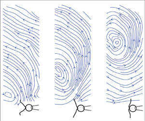
We illustrate the important differences between the stokeslet and the oscillet by representing the velocity fields associated with both singularities. Figure 1 illustrates the velocity field and streamline pattern for a point force located at the origin and oscillating along the  $x$-axis. Figure 1(a) corresponds to an oscillating stokeslet, while figure 1(b) corresponds to an oscillet. For the stokeslet, it is noteworthy that the $x$-component of the velocity field $\boldsymbol {u}$ has the same sign in the entire domain and remains always the same as the sign of the point force $\boldsymbol {F}$. The oscillet flow, figure 1(b), resembles the stokeslet flow only in the immediate vicinity of the origin, where the point force is located. The flow field is characterized by the presence of a stagnation point and that of closed streamlines around the stagnation point. The flow direction is therefore not uniform in the entire field. Along the $y$-axis, the sign of the velocity component $u$ changes beyond the stagnation point, which corresponds to a flow inversion point. This stagnation point moves away from the origin, figure 1(b, panels 1 to 5). A new stagnation point is generated at the origin, every time the point force changes direction, figure 1(b, panel 6). This new stagnation point, then, moves away from the origin, figure 1(b, panel 6–8). The propagation of the stagnation point is related to the diffusion of vorticity, which we consider next.

Figure 1. Streamlines deduced from the velocity field of a stokeslet with oscillating force (a) and that of an oscillet (b). The oscillating force  $F\sin (2{\rm \pi} t/T)$ is represented by the black arrow at the origin. From panel 1 to 8, $t/T$ = 0.03, 0.10, 0.20, 0.28, 0.39, 0.52, 0.60, 0.70. Grey arrows represent the velocity vector field.
Figure 2 represents the  $z$-component of the vorticity field in the $xy$-plane at different instants during a cycle. For a stokeslet, the vorticity field has a uniform sign in the entire field and is positive (respectively negative) for a positive (respectively negative) point force $\boldsymbol {F}$, figure 2(a). The vorticity field of the oscillet does not have a uniform sign. Vorticity is generated at the origin, figure 2(a, panel 1), and diffuses into the field, see panels 1–5. When the force direction reverses and becomes negative, negative vorticity is then generated at the point force, figure 2(a, panel 6), but the vorticity remains positive in the rest of the field.

Figure 2. Vorticity field,  $\boldsymbol {\omega } = \boldsymbol {\nabla } \times \boldsymbol {u}$, of a stokeslet with oscillating force (a) and that of an oscillet (b). Panels are taken at the same instants as in figure 1 respectively.
Finally, in the oscillet flow, there is phase delay between the oscillation of the flow velocity and the oscillation of the point force. This is not the case for the stokeslet flow. Figure 3 represents  $\theta _u$, the phase delay between $u$ and the point force. A distinct feature is that the phase increase is not isotropic. The phase increases slowly along the direction of the forcing, the $x$-axis, and significantly faster along directions perpendicular to the forcing, the $y$- and $z$-axis, see figure 3(b). It bears emphasis that the increase in phase delay occurs already at short distances from the point force, and is not limited to the far field. In fact, the phase increases the fastest at distances smaller than the diffusive length scale $\delta$.

Figure 3. Phase shift  $\theta _u$ between the forcing and the $x$-component of the velocity, computed with (2.6). The point force is at the origin and oscillates along the $x$-axis. (a) Phase shift in $xy$-plane. (b) Phase shift $\theta _u$ along the $x$- (red) and the $y$-axis (blue), corresponding to the horizontal and the vertical dashed line in (a) respectively. Axes are scaled by $\delta = \sqrt {\mu \tau /\rho }$.
3. Methodology
3.1. Optical tweezers velocimetry (OTV)
We measure the flow field around beating biological cilia. In nature, cilia beat at frequencies ranging from 10 to 100 Hz and generate flows with rich temporal dynamics. Resolving such dynamics requires high temporal and spatial accuracy. On these scales, velocimetry techniques based on passive tracers, such as particle image velocimetry (PIV) and particle tracking velocimetry (PTV) become inappropriate because the advection of passive tracers cannot be distinguished from Brownian motion (Meinhart, Wereley & Santiago Reference Meinhart, Wereley and Santiago1999). While the displacements due to the advection of the particle by the flow scale with  ${\sim }U\tau$, the displacements due to diffusion scale with ${\sim }\sqrt {D\tau }$, where $D$ is the diffusion coefficient of the tracer particle. The ratio of these length scales defines the Péclet number $Pe \sim U\sqrt {\tau /D}$, which represents a signal to noise ratio for passive tracer-based velocimetry. For smaller values of $Pe$, both PIV and PTV can still be used to measure the average flow, but they cannot accurately capture the unsteady nature of the flows. These physical limitations of micro-PIV can be reduced to a certain extend by using larger tracers, or in case of preknowledge of the periodic character of a flow, by using correlation averaging within a class of image pairs grouped to correspond to a given phase of the periodic flow, see Poelma et al. (Reference Poelma, Vennemann, Lindken and Westerweel2008). For unsteady ciliary flows, $Pe$ can be of order one and even much smaller at increased distances from the cilia. For such flows, the use of PIV and PTV is extremely difficult. Here, we tackle this challenge by using OTV (Wei et al. Reference Wei, Dehnavi, Aubin-Tam and Tam2019; Dehnavi et al. Reference Dehnavi, Wei, Aubin-Tam and Tam2020). Previously, optical tweezers have been employed to measure velocity of steady flows (Almendarez-Rangel et al. Reference Almendarez-Rangel, Morales-Cruzado, Sarmiento-Gómez, Romero-Méndez and Pérez-Gutiérrez2018). In this study, we leverage the high spatial-temporal resolution of the optical tweezers-based measurement to resolve both the steady and the unsteady component of the ciliary flow. In this technique, a bead is trapped by a focused laser beam. The local flow velocity directly relates to the displacement of the bead from the laser focal point. The desired temporal resolution in measuring the flow ( $\lesssim$0.1 ms) is achieved by using back focal plane interferometry (Gittes & Schmidt Reference Gittes and Schmidt1998; Farré, Marsà & Montes-Usategui Reference Farré, Marsà and Montes-Usategui2012) in monitoring the bead position $\Delta \boldsymbol {x}(t)$.
The OTV experimental setup is presented in figure 4(a,b) and is briefly summarized hereafter. Two laser beams are aligned and focused by a water immersion objective ( $\textrm {NA}=1.20$, 60 $\times$). A Nd:YAG ( $\lambda =1064$ nm) laser is used to trap spherical polystyrene beads of radii $a=0.5\text {--}2.5$ ${\rm \mu}$m at the focal point. Following Dehnavi et al. (Reference Dehnavi, Wei, Aubin-Tam and Tam2020), we use larger beads in a weaker trap to measure the small amplitude flows far away from the cell, and smaller beads with stronger traps to measure, with a higher spatial resolution, the flows closer to the flagella. As the beads vary in size, even within the same sample, we measure the size of each bead for each flow measurement. Back focal plane interferometry is performed with a second detection laser ( $\lambda =880$ nm), which is used to detect the position of the bead with a position sensitive detector (PSD, First Sensor DL100-7) (figure 4a). The experimentally acquired electrical signal from the PSD is converted into bead position following the same methodology as Lang et al. (Reference Lang, Asbury, Shaevitz and Block2002). The bead position $\Delta \boldsymbol {x}$ can be directly related to the local flow velocity $\boldsymbol {u}$, by considering the force balance between the force due to the optical tweezers $\boldsymbol {F}_{t} = -k \boldsymbol{\varDelta} \boldsymbol{x}$, and the hydrodynamic force $\boldsymbol {F}_{h}(t)$ due to the external flow $\boldsymbol {u}$, where $k$ is the stiffness of the optical tweezers. The Reynolds number of the bead, $Re_{a} = \rho |\boldsymbol {u}| a / \mu$, is small $Re_{a} \approx 10^{-5}\text {--}10^{-4}$, such that the hydrodynamic force on the bead reduces to the viscous drag only, and the flow velocity can hence be deduced from the equation
 \begin{equation} \frac{\textrm{d} \boldsymbol{\varDelta} \boldsymbol{x}}{\textrm{d}t} + \frac{k}{\gamma} \boldsymbol{\varDelta}\boldsymbol{x} = \boldsymbol{u}(t), \end{equation}
where  $\gamma =6{\rm \pi} \mu a$ is the Stokes drag coefficient. Using (3.1), we deduce the local flow velocity $\boldsymbol {u}(t)$ from the bead displacements $\boldsymbol{\varDelta} \boldsymbol {x}(t)$ using a Kalman filter, see Dehnavi et al. (Reference Dehnavi, Wei, Aubin-Tam and Tam2020) for detail.

Figure 4. Optical tweezers velocimetry (OTV) (a) Scheme of OTV. Lasers are used for trapping beads and detecting the beads’ displacement. Information on the bead's displacement is obtained by back focal plane interferometry, which is facilitated by a condenser and a position sensitive detector (PSD). (b) Zoom-in of the dashed circle in (a). The recovery force  $\boldsymbol {F}_{t}$ exerted by the optical tweezers equals the hydrodynamic force $\boldsymbol {F}_{h}(t)$. (c) Schematics showing how the biological sample is loaded. A customized flow chamber in a semi-circle shape of 15 mm diameter with a 2 mm thickness is used for experiments. Cells with beating cilia are captured by suction force applied through a glass micro-pipette. The cell and the pipette are mounted on a micro-manipulator which controls their relative position with respect to the laser trap. (d) Experimental configuration. A bead is optically trapped nearby to resolve the local flow velocities $u$ and $v$. The ciliary shapes during a typical beat are displayed. The ciliary phase $\phi \in [0,2{\rm \pi} )$ is used to describe the shapes, with the most forward-reaching shape defined as $\phi =0$. Inset shows a light microscope image of the corresponding experiment, in which the ciliary shapes correspond to approximately $\phi =0$.
3.2. Experimental setup and measurement settings
Wildtype Chlamydomonas reinhardtii cells (cc-125 mt+) cultured in TRIS-minimal medium ( $\textrm {pH}=7.0$) are used as biological samples to generate ciliary flows. In the OTV experiments, cell suspensions ( ${\sim }2 \times 10^4$ cells ml $^{-1}$) with uncoated polystyrene beads ( ${\sim }1 \times 10^5$ ml $^{-1}$) are filled into the custom-made flow chambers, see figure 4(c). The flow chamber is a semi-circle of 7.5 mm radius in the $xy$-plane and is 2.0 mm in height in $z$. Single cells are captured by suction force applied through custom-made micro-pipettes, figure 4(c,d). The openings of the pipettes are of 2–5 ${\rm \mu}$m diameter. As shown in figure 4(a), the pipette is held by a micro-manipulator (SYS-HS6, WPI) and can be moved in $x$,
$x$,  $y$, and $z$ directions with $\sim$1 ${\rm \mu}$m precision. With this, the cells are placed at different measurement locations with respect to the trapped bead. Unless otherwise mentioned, the ciliary beating plane is always aligned with the $xy$-plane. To record the ciliary beating of the captured cell, we use bright-field microscopy and high speed videography using an sCMOS camera (LaVision PCO.edge) at frame rates of 400–1400 fps. At each location, OTV measurement was carried out at a sampling frequency of 10 kHz and lasted 5–10 s.
A typical experimental configuration is displayed in figure 4(d), with a light microscope image from our experiments in the inset at the top right. The captured cells are held at 120  ${\rm \mu}$m above the bottom of the flow chamber. To prevent background flows due to evaporation during experiments, we seal the flow chamber with a layer of silicone oil. We record the flow velocity $\boldsymbol {u} (\boldsymbol {r},t)$ sequentially at a series of locations with respect to the cell $\boldsymbol {r}_i$ ( $i=1,2,3,\ldots$). The point where the cilia are anchored to the cell body is taken as the origin of the Cartesian coordinate system. The asymptotic behaviour of the flow along different axes, and the flow field over the $xy$-plane, are studied with different sets of sampled flow velocity $\boldsymbol {u} (\boldsymbol {r}_i,t)$ ( $i=1,2,3,\ldots$).
In addition to the OTV measurement, we simultaneously track the shapes of the beating cilia from the video recordings, figure 4(d). We define the ciliary phase  $\phi \in [0,2{\rm \pi} )$ to describe the shapes, with the most forward-reaching shape defined as $\phi =0$ (inset of figure 4d). For each frame, we determine the phase associated with the ciliary shape. To do this, we first time stamp the beginnings of each ciliary beat by identifying the most forward-reaching ciliary shapes ( $\phi =0$) for consecutive beats, based on the video taken simultaneously with the measurement. Second, the ciliary phase between two marked instants is linearly interpolated between $0$ and $2{\rm \pi}$. Figure 5(d) displays the ciliary shapes that are marked by the user as $\phi =0$, and are considered as $\phi =0.5{\rm \pi}$ and ${\rm \pi}$ by interpolation, from left to right, respectively. The point clouds represent the corresponding shapes from different cycles, and the solid lines represent the median shapes. The narrow spans of the point clouds confirm the accuracy of the time-stamping.

Figure 5. Numerical method and signal post treatment. (a) Flow field is computed numerically with the BEM using tracked ciliary shapes shown in figure 4(d). (b,c) The axial ( $x$) and the lateral ( $y$) velocity component, $u$ and $v$, measured by OTV and computed by BEM. Raw OTV data are presented as grey dots in the background, while blue lines show the signal after moving window average (MWA). BEM computations are overlaid in red. A typical beat is shaded, which begins with the most forward-reaching ciliary shapes ( $\phi$=0). (d) Accuracy of the time-stamping method. Grey dots represent the shapes stamped as $\phi =0$, $0.5{\rm \pi}$, and ${\rm \pi}$, respectively. Black lines represent the median shapes. (e, f) The average cycle of $u$ and $v$. Solid lines and the shadings represent the median and the interquartile range for flows sample over $\sim$40 cycles. All flow velocities are scaled by $U_0=L f\approx 600$ ${\rm \mu}$m s $^{-1}$.
3.3. Boundary element method (BEM) and slender-body theory
To compute the flow velocity predicted by the Stokes equations (2.3), a hybrid method combining the BEMand slender-body theory (SBT) (Keller & Rubinow Reference Keller and Rubinow1976) is employed. For simplicity, in the following parts, we refer to this method as the BEM, and it will be later further integrated with direct numerical simulation (DNS) to compute the flow field (§ 5.2).
In this BEM approach, the cell body and the pipette are represented as one entity, with a completed double layer boundary integral equation (Power & Miranda Reference Power and Miranda1987). Stresslet singularities are distributed on the surface of the cell-pipette, while the stokeslet and rotlet singularities of the completion flow are distributed along the centerline of the cell-pipette (Keaveny & Shelley Reference Keaveny and Shelley2011). The no-slip boundary condition on the cell-pipette surface is satisfied at the collocation points. The cilia are represented using slender-body theory (Keller & Rubinow Reference Keller and Rubinow1976) with 26 discrete points along each of the cilium's centerline. The time-dependent motion of each of the 26 discrete points on a beating cilium are tracked from video, following a procedure similar to Riedel-Kruse et al. (Reference Riedel-Kruse, Hilfinger, Howard and Jülicher2007) and Geyer et al. (Reference Geyer, Jülicher, Howard and Friedrich2013).
For each computation, we adjust the size of the pipette opening and the cell body shape according to the corresponding experiment. Realistic ciliary shapes are tracked from the video frames (figure 4d) and represented using SBT. The flow field corresponding to each frame is then computed. Figure 5(a) shows the computed flow field in the middle of the power stroke. Computed velocity  $\boldsymbol {u}_{S}(t)$ at the bead's position (the white circle) is displayed in figure 5(b,c). The computed signals (red) are overlaid with the OTV results (grey and blue), showing the great accuracy of the numerical method. Flow velocities are scaled by $U_0=Lf$, with $L$ and $f$ the ciliary length and frequency.
Because  $\boldsymbol {u}_{S}(t)$ is computed by solving the Stokes equations (2.3), where the entire fluid domain is in phase with the forcing, in the following sections, $\boldsymbol {u}_{S}(t)$ is regarded as the reference signal and its phase represents the phase of the forcing (ciliary beating).
4. Asymptotic behaviour of the flow field around beating cilia
We start by investigating the asymptotic behaviour of the flow field around beating cilia, which includes the rates of spatial decay in the near field and far field of both the steady and the unsteady component of the ciliary flow, and the rate of spatial phase shift of the unsteady component. We measure the ciliary flow along the  $x$-,
$x$-,  $y$-, and $z$-axis, by sampling flow velocities along ( $x$,
$x$,  $0\pm 5$ ${\rm \mu}$m, 0), ( $0\pm 5$ ${\rm \mu}$m, $y$, 0), and ( $0\pm 5$ ${\rm \mu}$m, $0\pm 5$ ${\rm \mu}$m, $z$), respectively. The uncertainties of $\pm$5 ${\rm \mu}$m result from aligning the measurement locations to the origin (the anchor point of cilia, figure 4d). Each dataset presented consists of 8–30 sampled points along a specific axis for a given cell. In total, the present study includes $N=30$ cells and $N=38$ datasets. Note that some cells were used to study the flow behaviour along more than one axis. Each cell is consistently represented by a specific symbol throughout the figures in this section. Most measurements are performed within a maximum distance of $\sim$160 ${\rm \mu}$m and a minimum distance of ${\sim }L+5$ ${\rm \mu}$m from the origin, where $L$ is the cilium length of each cell. $L$ varies from 8 to 18 ${\rm \mu}$m over the cells used in this study, and the average is $\bar {L}=12$ ${\rm \mu}$m. This minimum distance of ${\sim }L+5$ ${\rm \mu}$m is chosen to avoid interference of the trapping laser and the trapped bead with the ciliary beating. We present a systematic study of the behaviours of both the axial and the lateral flow components along different axes. We compare the experimentally observed asymptotic behaviours to those of the reduced theoretical models of systems of stokeslets and oscillets, which sheds light on the nature of the ciliary flow. Practically, this knowledge can help build more accurate models in simulation, and hence potentially help us better understand ciliary synchronization.
4.1. Amplitude of the steady component
We first discuss the measurements of the steady component, i.e. the average flow. Figure 6 displays the axial average flow  $\bar {u}$ along the $x$-,
$x$-,  $y$-, and $z$-axis, and the lateral average flow $\bar {v}$ along the $y$-axis, respectively. Due to the symmetry of the breaststroke, $\bar {v}$ along the $x$- and $z$-axis are approximately zero and therefore are not presented. The measurement settings are displayed by the schematics in each panel. Different markers represent different cells. Flow velocities are scaled by $U_0=L f$, with $L$ and $f$ the ciliary length and frequency, as $U_0$ accounts for the different sizes and frequencies over different cells. Distances are scaled by the characteristic length of vorticity diffusion $\delta =\sqrt {\mu / \rho f} \approx 140$ $\mu$m.

Figure 6. (a–c) Axial average flow ( $\bar {u}$) measured along the $x$-,
$x$-,  $y$-, and $z$-axis. (d) Lateral average flow ( $\bar {v}$) measured along the ( $\sim$2 ${\rm \mu}$m, $y$, 0), which is close to but slightly deviates from the $y$-axis. Measurement configurations are shown by the schematics respectively. Flow velocities are scaled by $U_0=L f\approx 600$ ${\rm \mu}$m s $^{-1}$. Distances are scaled by $\delta \approx 140$ ${\rm \mu}$m. Different markers represent different cells. Dashed lines: flow amplitudes of Blake's solution for a forcing strength $F=23.3$ pN.
We find that both  $\bar {u}$ and $\bar {v}$ follow a $1/r$ decay along the $x$-,
$x$-,  $y$- and $z$-axis, figure 6, in agreement with Drescher et al. (Reference Drescher, Goldstein, Michel, Polin and Tuval2010) and Guasto et al. (Reference Guasto, Johnson and Gollub2010). The experimental velocity measurements can be compared with the solution to the Stokes equations for a point force in the $x$-direction and located $h=120\ {\rm \mu}\textrm {m} \approx 0.8\delta$ above a no-slip wall, obtained from the Blake tensor (Blake Reference Blake1971). The dashed lines in figure 6 represent the amplitudes of the average flow along the different axes, computed with the Blake tensor, for a forcing strength of $F=23.3$ pN, corresponding to the force exerted by both flagella. We see that the rates of the spatial decay ( $1/r$) are captured quantitatively for $r < h \approx 0.8\delta$. For distances $r$ on the same order of magnitude as $h$, the spatial decay rate increases, which is consistent with the presence of the no-slip wall, see Blake's solution in figure 6(b). It is worth noticing that the flow amplitudes within the $xy$-plane are predicted accurately and simultaneously with the same point force (figure 6a,b,d). This indicates that the average flow created by captured C. reinhardtii cells within the ciliary beating plane can be accurately represented by a single stokeslet (Brumley et al. Reference Brumley, Wan, Polin and Goldstein2014). Lastly, we find the velocity magnitude to be smaller in the $z$-direction normal to the beating $xy$-plane, compared to the $y$-direction. This highlights the limitations of representing a cilium beating in a plane with an axisymmetric stokeslet.
4.2. Amplitude of the unsteady component
We now discuss the unsteady component of ciliary flow, or the oscillatory flow,  $\boldsymbol {u}' = \boldsymbol {u}- \bar {\boldsymbol {u}}$. By definition, it generates zero net flow per cycle, and we thus report the decay of the amplitude of the oscillations, $\delta \boldsymbol {u}'$ computed as half of the peak-to-peak amplitude of $\boldsymbol {u}'$. Figure 7 represents the axial ( $\delta u'$) and the lateral ( $\delta v'$) amplitude of the oscillatory flow, along the $x$-,
$x$-,  $y$-, and $z$-axis. Cells are represented by the same symbols as used in figure 6. The important observation is that the asymptotic behaviour of the unsteady component differs markedly from that of the corresponding average component. The rates of spatial decay of the unsteady component are higher, see figure 7. While the amplitude of the average flow decays in $1/r$, the amplitude of the flow oscillations decays at a rate close to $1/r^3$. This difference in the asymptotic behaviours between the average ( $\bar {u},\bar {v}$) and the oscillatory ( $u',v'$) flow suggests that they are not governed by the same equations. A $1/r$ rate of decay is consistent with the stokeslet solution to the Stokes equations, while a higher rate of decay observed is consistent with the oscillet solution to the unsteady Stokes equations. Further features are reminiscent of the oscillet solution. The spatial decay of $\delta u'$ becomes stronger than $1/r$ at shorter distances along the $y$- and $z$-axis, which are normal to the point force, compared to the $x$-axis, see figure 7(a–c). This is also the case for the oscillet (2.6). The decrease of $\delta v'$ along the $y$-axis, figure 7(d), is stronger than that of $\delta u'$ along the $x$-axis, figure 7(a), at short distances from the cilia. This is due to the fact that we measure the flow generated by two cilia, beating in an antisymmetric breaststroke. In the $x$-direction, the cilia beat in the same direction and the flow generated by each cilium in the $x$-direction contributes to the velocity $u$. In the $y$-direction on the other hand, the cilia beat in antisymmetric fashion, and the flows generated by each cilium tend to cancel each other out, leading to the observed faster rate of decay. It is noteworthy that along the $y$-direction, $\delta u'$ and $\delta v'$ are of similar amplitude in the vicinity of the cell, where the measured flow is predominantly created by the closest cilium figure 7(b,d). This is in contrast to the average flow, for which $\bar {u}$ is significantly larger than $\bar {v}$, figure 6(b,d). Therefore, the unsteady flow created by one beating cilium corresponds to oscillating forces along both the $x$- and the $y$-directions.
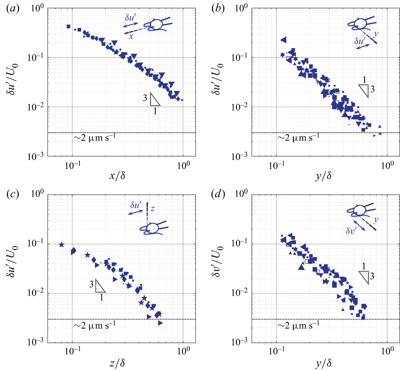
Figure 7. (a–c) Amplitude of the axial oscillatory flow ( $\delta u'$) measured along the $x$-,
$x$-,  $y$-, and $z$-axis. (d) Amplitude of the lateral oscillatory flow ( $\delta v'$) measured along the $y$-axis. The symbols for different cells are consistent with the ones used in figure 6.
4.3. Phase shift of the unsteady component
The higher rate of decay is not the only difference between the fundamental solutions of the Stokes and the unsteady Stokes equations. A defining feature of solutions to the unsteady Stokes equation is the phase lag between the oscillations of the flow velocity and the forcing, which develops at increasing distances from the forcing. This phase lag is a characteristic of Stokes’ second problem as well as of the oscillet. Here we measure this phase lag and present its asymptotic behaviour along different axes.
Figure 8 demonstrates the phase shift of the axial flow velocity at two locations along the  $y$-axis. The OTV measurements, $u$ (grey and blue), are overlaid with the BEM computations, $u_{S}$ (red), which assume the flow to satisfy the Stokes equations, figure 8(a,b). Close to the cilia, $r=y=23.0\ {\rm \mu}\textrm {m} \approx 0.16\delta$; the computed flow reproduces the measured flow accurately: they have the same amplitude and reach maximum and minimum simultaneously, figure 8(a). Farther away, at $r=y=66.2\ {\rm \mu}\textrm {m} \approx 0.47\delta$, the amplitude of the measured oscillatory flow velocities is lower, and the oscillations are phase-shifted compared to the Stokes computations, figure 8(b) and inset. The phase shift is approximately ${\rm \pi} /2$ and the two signals are in quadrature.

Figure 8. The flow velocity is phase-shifted at increasing distance. (a) Close to the cell on the lateral ( $y$) side, $y=23.0\ {\rm \mu}\textrm {m} \approx 0.16\delta$, experimental and computational results are in phase. (b) At a larger distance, $y = 66.2\ {\rm \mu}\textrm {m}\approx 0.47\delta$, the measured signal is phase-delayed. Inset: OTV raw data (grey), moving-window-averaged data (blue), and flow computed by BEM (red). (c,d) Using the cross-correlation function $C(\phi ')=u(\phi +\phi ') \star u_{S}(\phi )$ to quantify the phase shift between the OTV signal $u(\phi )$ and the BEM computation $u_{S}(\phi )$. ${\bar {C}(\phi')}$ is the correlation $C(\phi ')$ normalized. (a,b) Reprinted figure with permission from Wei et al. (Reference Wei, Dehnavi, Aubin-Tam and Tam2019). Copyright (2019) by the American Physical Society.
We quantify the spatial phase shift of ciliary flow by computing the cross-correlation function between the flow measured by OTV and that computed by BEM. For each recording, we proceed by first determining the ciliary phase  $\phi (t)$ as described in the methodology section. This allows us to transform the measured and the computed time series of flow velocity, $u(t)$ and $u_{S}(t)$, as functions of the ciliary phase $\phi$, or $u(\phi )$ and $u_{S}(\phi )$. Then, we compute the cross-correlation function $C(\phi ')=u(\phi +\phi ') \star u_{S}(\phi )$. The phase shift between the measured velocity and the velocity predicted by the Stokes equations corresponds to the phase for which the cross-correlation function reaches a maximum, $C_{max}= C(\phi _{shift})$. In figure 8(c,d) we plot the normalized cross-correlation function, $\overline{C(\phi')} = C(\phi ')/C_{max}$, between the signals shown in figures 8(a) and 8(b), respectively. In the vicinity of the cell, $r \approx 0.16\delta$, $\phi _\textrm {{shift}} \approx 0$; while at a larger distance, $r \approx 0.47\delta$, $\phi _\textrm {{shift}} \approx \pi /2$.
We further characterize the phase shift of both the axial ( $u'$) and the lateral ( $v'$) oscillatory flow, along the $x$-,
$x$-,  $y$-, and $z$-axis, and over the $xy$-plane. For consistency and simplicity, we denote the spatial phase shift $\phi _{shift}$ of $u$ and $v$ as $\theta _u(\boldsymbol {r})$ and $\theta _v(\boldsymbol {r})$ respectively in the following parts.
In figure 9 we present  $\theta _{u}$ along the $x$,
$x$,  $y$, and $z$-axis, and $\theta _{v}$ along the $y$-axis, respectively. Cells are represented by the same symbols as used in figures 6 and 7. For each case, there is a clear phase shift between the measured flow and the forcing, which increases with the distance to the cilia. The increase of this phase-delay is highly dependent on the direction, as can be seen from the different slopes in figure 9. The phase-delay is 2–3 times stronger along directions perpendicular to the oscillating velocity, compared to the direction of the oscillating force. Quantitatively, the slopes for $\theta _u$ along the $x$-axis and $\theta _v$ along the $y$-axis are $0.30{\rm \pi} /\delta$ and $0.52{\rm \pi} /\delta$, respectively, figures 9(a) and 9(d); while the slopes for $\theta _u$ along the $y$- and the $z$-axis are $1.08{\rm \pi} /\delta$ and $1.16{\rm \pi} /\delta$, respectively, figures 9(b) and 9(c). The significant difference in the phase-delay along the different directions agrees with the oscillet solution. The dashed line in each panel represents the corresponding phase shift predicted by an oscillet located at the origin (figure 3b). Figure 9(a–c) correspond to an oscillet with oscillating force along the $x$-axis and figure 9(d) corresponds to an oscillet with oscillating force along the $y$-axis. The predictions are in agreement with the experimental results. Note that the resemblance between $\theta _u$ along $y$- and $z$-axis (figure 9b,c) reflects the axisymmetry of an oscillet (2.6).

Figure 9. (a–c) Phase delay of the axial oscillatory flow ( $\theta _{u}$) along the $x$-,
$x$-,  $y$-, and $z$-axis. (d) Phase delay of the lateral oscillatory flow ( $\theta _{v}$) along the $y$-axis. Dashed lines: corresponding phase delay predicted by an oscillet located at the origin, with oscillating force along the $x$-axis (a–c) and the $y$-axis (d), respectively. The symbols for different cells are consistent with the ones used in figures 6 and 7.
5. Unsteady velocity fields in the beating plane of cilia
In the previous section we have systematically studied the asymptotic behaviours of the flow created by beating cilia and found them to be in qualitative agreement with the oscillet. We further proceed to resolve the spatiotemporal features of the entire flow field around beating cilia and perform time-resolved direct numerical simulations (DNS) to compare with our measurements and the BEM simulations.
5.1. OTV measurements of the entire flow field
The time-resolved flow field over the  $xy$-plane is reconstructed from measurements performed at points $\boldsymbol {r}_i$ on a rectangular grid on one side of a cell. The grid covers the area where $x \in [-30,30]$ ${\rm \mu}$m and $y \in [0, 160]$ ${\rm \mu}$m with a grid size of 10 ${\rm \mu}$m. In total, there are N = 78 sampling points. At each point, OTV measurements were carried out at 10 kHz for 5 s, and high speed videography was performed simultaneously at a frame rate of 669 Hz. Each recording is time-stamped in order to construct the ciliary phase $\phi$ for $\sim$40–50 consecutive beats, following the methodology detailed previously (§ 3.2). The time series of velocity measurements are interpolated at N = 20 equally spaced phases $\phi _j$ ( $\,j=1,2,\ldots ,20$) between $\phi =0$ and $2{\rm \pi}$, and the velocity measurements over the consecutive beats are binned for each of the phases $\phi _j$. The flow velocity $\boldsymbol {u}(\boldsymbol {r}_i,\phi )$ at each measurement location $\boldsymbol {r}_i$, is calculated as the median of the marked cycles. Figure 5(e, f) display the median flow velocity cycles and the interquartile ranges that are calculated based on the signals shown in figure 5(b,c). Snapshots of the flow velocity field on the $xy$-plane for each phase $\phi _j$ are obtained through two dimensional linear interpolation of the velocity between the sampling points $\boldsymbol {r}_i$.
Figure 10 represents the time-resolved flow field around a single captured cell. The panels show the reconstructed flow field at different instants that correspond approximately to the shown ciliary phase  $\phi$ . The vector field represents the velocity field, and the contours represent the magnitude of the velocity.

Figure 10. Ciliary flow field measured experimentally. Snapshots of flow field are taken at the time when the cilia display shown shapes. Vector field: flow velocity; contour: flow speed. Both axes are scaled by  $\delta =\sqrt {\mu / \rho f} \approx 140$ ${\rm \mu}$m. Data corresponding to the experimentally measured velocity field are available through the 4TU.center for research data (Tam & Wei Reference Tam and Wei2021).
5.2. Numerical simulation: DNS-BEM method
We perform direct numerical simulations (DNS), which solves the Navier–Stokes equations (2.1), in order to compare these with our measurements of the unsteady velocity field. The DNS solution includes the effects of all terms of Navier–Stokes equations, including the unsteady and the nonlinear ones, see (2.1). Here, we use a structured Cartesian grid. The implementation of our numerical approach makes use of the BEM solution, described earlier in § 3.3, to propagate the no-slip boundary condition to the grid point immediately surrounding the fluid/solid interface.
We do this by dividing the computational domain into an inner and an outer region. The inner region corresponds to the flow domain in the direct vicinity of the cilia, the cell body and the pipette, see region marked pink and grey in figure 11. In this region, the Stokes equations remain valid, and the solution on the nodes within this region is computed using the BEM method described in § 3.3, which appropriately imposes the no-slip boundary condition at the surfaces of the cilia, the cell body and the pipette. This allows the no-slip boundary condition to be transferred to the neighbouring grid nodes. In practice, the inner region includes the nodes covered by the cell and the pipette, the nodes swiped across by the cilia during a beat and the nodes within two grid cells outwards from these (pink region in figure 11).

Figure 11. Schematic of the computational domain for the DNS-BEM simulations. The total domain size is 720  ${\rm \mu}$m in the $z$-direction and 1440 ${\rm \mu}$m in the $x$- and $y$-directions, with a grid size of 4 ${\rm \mu}$m. The cell is located in the center of the computational domain. The red shaded region corresponds to the area where the OTV experiments are performed. The inset shows the inner and outer regions. Within the inner region (coloured with grey and pink), the velocity is computed by the BEM method and used as velocity boundary conditions for the DNS simulations. For the rest of the domain, the velocity is computed with DNS with all boundary conditions shown.
The outer region corresponds to the rest of the computational domain, which represents the space between  $x=0$ and $x=1440$ ${\rm \mu}$m, $y=0$ and $y=1440$ ${\rm \mu}$m, and $z=0$ and $z=720$ ${\rm \mu}$m. In the outer region, the Navier–Stokes equations (2.1) are solved using the finite volume scheme, operator splitting and the solenoidal projection technique (Pozrikidis Reference Pozrikidis2016), on a staggered grid with discretization size of 4 ${\rm \mu}$m. A second-order Adams–Bashforth scheme is used for explicit time integrations. Lastly, free slip boundary conditions are applied on $z=0$ and $z=720$ ${\rm \mu}$m, and fully developed boundary conditions on $x,y=0$, $x,y=1440$ ${\rm \mu}$m, as shown in figure 11. We confirm that the size of the computational domain is large enough so that the boundary conditions on the edge of the domain have a negligible effect on the flow velocity within our experimentally measured region (the red rectangle in figure 11).
5.3. Phase shift over the ciliary beating plane
We have previously highlighted the anisotropy in phase lag along axes parallel and normal to the force direction (§ 4.3). Here, we consider the axial component of the oscillatory flow ( $u'$) and present the spatial phase shift ( $\theta _{u}(x,y)$) between the flow velocity measured experimentally and computed by the DNS-BEM approach, see figure 12.

Figure 12. (a) Experimentally measured phase shift of the axial oscillatory flow over the ciliary beating plane, or  $\theta _{u}(x,y)$. (b) Same phase shift computed by the DNS-BEM approach.
From the experimental results shown in figure 12(a), we see that the contours of equal phase shift are not conspherical, i.e. the increase in phase is not isotropic. They have a notch shape or a V-shape in the  $y$-direction normal to the force direction. This feature indicates that the phase shift increases the fastest along the lateral ( $y$) direction and the slowest along the axial ( $x$) direction, as shown in figure 9(a–c), and that the phase shift along $x\approx -0.1\delta$ is the maximum. The phase lag in the velocity field therefore strongly depends on the relative spatial position. Due to the axisymmetry between the $y$ and $z$, the phase shift contour in the $xz$-plane is expected to be the same as our results for the $xy$-plane, while the contours of equal phase over the $yz$-plane are expected to be concentric circles.
The measured phase lag field (figure 12a) is similar to the one predicted by the oscillet solution (figure 3a) and in quantitative agreement with the phase lag field computed from our simulations (figure 12b). For both experiments and simulations, the V-shape equal phase contours have a maximum phase shift along  $x\approx -0.1\delta$. These results have implications in studies of hydrodynamic synchronization between cilia. The oscillatory flow has the strongest contribution to the hydrodynamic interaction and is 2–5 times larger in amplitude than the average flow, see figures 6 and 7.
5.4. Vorticity diffusion
Finally, we characterize spatiotemporal features of the flow field around beating cilia in the  $xy$-plane. As discussed in § 2.1, the fundamental difference between the steady and the unsteady Stokes equations is the quasi-steady assumption, which neglects the time scale for vorticity (momentum) to diffuse. We deduce the vorticity field from the point measurements of the velocity (figure 13). Snapshots of the vorticity field at different times during a ciliary beat are presented for the unsteady velocity fields measured experimentally and for the fields computed by the DNS and the BEM approach in figures 13(a), 13(b), and 13(c) respectively. From left to right, columns 1–5 are during the power stroke and 6–8 the recovery stroke.

Figure 13. Vorticity field measured experimentally (a), and computed with the DNS (b) and the BEM (c). The vorticity  $\boldsymbol {\omega } = \boldsymbol {\nabla } \times \boldsymbol {u}$ at different times during the power stroke and the recovery stroke are displayed. Corresponding ciliary shape and ciliary phase $\phi$ are shown for each panel. Grey arrows: the unsteady velocity component. Data corresponding to the experimentally measured (a) and computed (b) vorticity fields are available through the 4TU.center for research data (Tam & Wei Reference Tam and Wei2021).
The computed vorticity field around a beating cilium (figure 13b,c) can be compared with the those of the stokeslet and the oscillet (figure 2a,b). The no-slip boundary conditions on beating cilia lead to more complex spatiotemporal patterns than the point forces. The vorticity fields are not symmetric around the  $x=0$ axis while the fields associated with the point-force are. The sign of vorticity changes in front of the cilia, at $x\approx -0.1\delta$, see figure 13, at $\phi / 2 {\rm \pi}= 0.08$ at the beginning of the power stroke and at $\phi / 2 {\rm \pi}= 0.58$ during the recovery stroke.
The BEM solution (figure 13c) differs from the DNS solution (figure 13b) similarly to how stokeslets differ from oscillets. This is best seen in the middle of the power stroke at  $\phi / 2 {\rm \pi}= 0.18$ and in the middle of the recovery stroke at $\phi / 2 {\rm \pi}= 0.68$. In both cases, the vorticity immediately surrounding the cilia has a different sign compared to that far away from the cilia at $y / \delta \ge 0.8$. This is due to the finite time required for the vorticity to diffuse, which is captured by the DNS solution (figure 13b) but not by the BEM solution solving the Stokes equations (figure 13c).
The vorticity field reconstructed from the OTV measurements (figure 13a) is most similar to the DNS simulations. The point of sign inversion in the vorticity field can be seen to diffuse away from the cilia, signifying the importance of taking into account the unsteady effect.
The agreement between the DNS simulations and the experimental measurements can be clearly seen when considering the director field of the flow velocity. To allow a better comparison with the oscillet, we represent the director field of the oscillatory component  $\boldsymbol{u}'$, for which the average flow has been subtracted. Figure 14 represents the streamlines associated with the $\boldsymbol{u}'$ field for the same snapshots as in figure 13. The pattern of streamlines obtained from the experimental data (figure 14a) is in agreement with the DNS simulations (figure 14b). Both include closed streamlines around a stagnation point, on each side of which the flow direction changes. These closed streamlines are clearly absent in the BEM simulations (figure 14c), which assume Stokes flow. The closed streamlines are created in the vicinity of the cilia at the beginning of both the power and recovery strokes, and propagate away from the cell along the $y$-axis, see figure 14. The streamline pattern has a typical signature, which is also in close agreement with that of the oscillet and very different from that of a stokeslet, see figure 1.

Figure 14. Velocity field measured experimentally (a), and computed with the DNS (b) and the BEM (c), visualized by streamlines. Data corresponding to the streamlines obtained from the measured (a) and computed (b) velocity fields are available through the 4TU.center for research data (Tam & Wei Reference Tam and Wei2021).
We quantify the time scale for the propagation of the closed streamlines away from the cilia. We do this by tracking the stagnation point at the centre of these closed streamlines  $(x_{o},y_{o})$, which also corresponds to the flow inversion point. The tracking of the inversion point is represented in figure 15 for the experimental fields, the DNS solution and the oscillet. The inset demonstrates how we mark the stagnation point, $(x_{o},y_{o})$ (red crosses). During the propagation, $x_{o}$ remains approximately unchanged, and we thus focus on $y_{o}$. We report the results for two typical cells presented with different markers. Our experimental measurements are in striking agreement with the DNS simulations and the oscillet. In all datasets, the stagnation point propagates to a distance of $r=\delta$ after approximately half a cycle. Thus, for C. reinhardtii, the diffusive time scale of vorticity is $\tau \approx 1/2f \approx 10$ ms.

Figure 15. The propagation of the stagnation point. Inset: two panels from left to right show the creation of the stagnation point and its propagation after approximately 1/4 cycle. The stagnation point is marked by the red cross:  $(x_{o},y_{o})$. Squares and circles: experiments performed with two different cells, with the squares representing the cell used for § 5. The shaded area marks the power stroke.
The measured time scale of vorticity diffusion also provides another way to consider the spatial phase shift of the unsteady flow. In figure 15, the linear best-fit to the experimental results gives a speed of vortex propagation of  $\textrm {d} y_{o}/\textrm {d}t = 2.10 \delta$ per cycle ( $2{\rm \pi}$). This is equal to a phase delay of $0.95{\rm \pi} /\delta$, which agrees well with the rate of phase shift $\theta _u$ along the $y$-axis reported previously in § 4.3, $\partial \theta _{u} / \partial y \approx 1.08{\rm \pi} /\delta$, see figure 9(b).
6. Conclusion
By exploiting the high spatial and temporal resolution of the OTV technique, we are able to systematically characterize the steady and unsteady components of the flow created by beating cilia. We first resolve the flows’ asymptotic behaviours along different axes, and compare those behaviours with fundamental solutions to the steady and unsteady Stokes equations. Finally, we characterize the unsteady velocity field over the entire ciliary beating plane to resolve its spatiotemporal dynamics. Experimental results are compared again with numerical simulations, and are found to be in agreement with the solution to the unsteady Stokes equations and to show significant differences with the solution to Stokes equations.
For the steady component of the ciliary flow, we find that the average velocity field can be well reproduced by the Stokes equations, in agreement with previous studies (Drescher et al. Reference Drescher, Goldstein, Michel, Polin and Tuval2010; Guasto et al. Reference Guasto, Johnson and Gollub2010). Moreover, for a captured C. reinhardtii cell, the average flow velocity generated by both flagella along the  $x$ and $y$ axes can be quantitatively reproduced with a single stokeslet of magnitude $F= 23.3\pm 8.3$ pN (mean $\pm$ std) and its image system due to the no-slip wall (Blake's solution). For the unsteady component (the oscillatory flow), we measure the rates of decay and the rates of phase shift along different axes. We show that they decay faster than the average flow, which indicates that the governing equations for these two components must be different, and we show that the decay rates are closer to those predicted by the unsteady Stokes equations.
We present the time-resolved ciliary flow field over the beating plane. Our experimental results reveal rich spatiotemporal dynamics of the unsteady velocity field. By comparing the experimental results with the computed flow fields of an oscillet, that from the direct numerical simulations (DNS) and that computed with the boundary element method (BEM), we are able to visualize and characterize the finite scale of vorticity diffusion. We discuss an important consequence of the finite time scale for vorticity diffusion, namely, the phase-lag between the velocity and the forcing.
In cilia carpets, the synchronization of cilia beating is characterized by metachronal rhythm, which originates from a spatially organized phase delay, between thousands of cilia. Our study shows that there is a simple phase delay built into the physics of hydrodynamic interactions, that could influence metachrony. We measure an increase in the phase delay due to the unsteady nature of the flow, which reaches  $1.16{\rm \pi} /\delta \approx 0.026$ rad ${\rm \mu}$m $^{-1}$. This value is comparable to the phase delay characterizing the metachronal wave in Volvox and reported in Brumley et al. (Reference Brumley, Polin, Pedley and Goldstein2012), while it is smaller than those observed in Paramecium (Funfak et al. Reference Funfak, Fisch, Abdel Motaal, Diener, Combettes, Baroud and Dupuis-Williams2014) or Schmidtea mediterranea (Rompolas, Patel-King & King Reference Rompolas, Patel-King and King2010). While the origin of metachrony remains unclear, an accurate representation of the hydrodynamic interactions between the cilia should account, in some cases, for the unsteady effects and the phase lag characterized here.
For oscillatory flows on the micro-scale, our results highlight the importance of taking into account unsteady effects, even over length scales which are shorter than the characteristic diffusive length scale  $\delta =\sqrt {\mu / \rho f}$. Indeed, the induced phase delays are already significant, and reaching ${\rm \pi} /2$ at distances $r\approx 0.5 \delta$. One particular example is the hydrodynamics of sperm cells, for which the beating frequencies range over 10–100 Hz and the length of the flagellum can reach 100 ${\rm \mu}$m. For such flows, unsteady effects may already be of importance and, in certain cases, non-local slenderbody theory may require a correction to take these into account.
Our results confirm the breakdown of the quasi-steady approximation assumed by the Stokes equations, and reveal the unsteady nature of ciliary flow field. The study highlights the limit of using stokeslets to represent unsteady flows generated by beating cilia, microswimmers and more generally oscillatory micro-scale flows. The study highlights that the fundamental solution to the unsteady Stokes equations, the oscillet (2.6), can be used to represent such unsteady flows.
Acknowledgements
The authors thank R. Kieffer for technical support.
Funding
The work was supported by the European Research Council (ERC Starting grant no. 716712) and the Netherlands Organization for Scientific Research (Frontiers of Nanoscience program).
Declaration of interests
The authors report no conflict of interest.
Author contributions
D. Wei and P.G. Dehnavi have contributed equally to this work. All authors designed the research. D. Wei conducted the experiments, analyzed the data, and drafted the manuscript. P.G. Dehnavi designed and performed the flow field computations. All authors revised the manuscript.


 Open access