


1. Introduction
Automatic differentiation (AD) is a popular technique for computing derivatives of functions implemented by computer programs, essentially by applying the chain rule across the program code. It is typically the method of choice for computing derivatives in machine learning and scientific computing because of its efficiency and numerical stability. AD has two main variants: forward-mode AD, which calculates the derivative of a function, and reverse-mode AD, which calculates the (matrix) transpose of the derivative. Roughly speaking, for a function
 $f:{\mathbb{R}}^n\to {\mathbb{R}}^m$
, reverse mode is the more efficient technique if
$f:{\mathbb{R}}^n\to {\mathbb{R}}^m$
, reverse mode is the more efficient technique if
 $n\gg m$
and forward mode is if
$n\gg m$
and forward mode is if
 $n\ll m$
. Seeing that we are usually interested in computing derivatives (or gradients) of functions
$n\ll m$
. Seeing that we are usually interested in computing derivatives (or gradients) of functions
 $f:{\mathbb{R}}^n\to\mathbb{R}$
with very large n, reverse AD tends to be the more important algorithm in practice (Baydin et al. Reference Baydin, Pearlmutter, Radul and Siskind2017).
$f:{\mathbb{R}}^n\to\mathbb{R}$
with very large n, reverse AD tends to be the more important algorithm in practice (Baydin et al. Reference Baydin, Pearlmutter, Radul and Siskind2017).
While the study of AD has a long history in the numerical methods community, which we will not survey (see, e.g., Griewank and Walther Reference Griewank and Walther2008), there has recently been a proliferation of work by the programming languages community examining the technique from a new angle. New goals pursued by this community include
-
• giving a concise, clear, and easy-to-implement definition of various AD algorithms;
-
• expanding the languages and programming techniques that AD can be applied to;
-
• relating AD to its mathematical foundations in differential geometry and proving that AD implementations correctly calculate derivatives;
-
• performing AD at compile time through source code transformation, to maximally expose optimization opportunities to the compiler and to avoid interpreter overhead that other AD approaches can incur;
-
• providing formal complexity guarantees for AD implementations.
We provide a brief summary of some of this more recent work in Section 16. The present paper adds to this new body of work by advancing the state of the art of the first four goals. We leave the fifth goal when applied to our technique mostly to future work (with the exception of Corollary 130). Specifically, we extend the scope of the Combinatory Homomorphic Automatic Differentiation (CHAD) method of forward and reverse AD (Vákár Reference Vákár2021, Vákár and Smeding Reference Vákár and Smeding2022) (from the previous state of the art: a simply typed
 $\lambda$
-calculus) to apply to total functional programming languages with expressive type systems, that is, the combination of:
$\lambda$
-calculus) to apply to total functional programming languages with expressive type systems, that is, the combination of:
-
• tuple types, to enable programs that return or take as an argument more than one value;
-
• sum types, to enable programs that define and branch on variant data types;
-
• inductive types, to include programs that operate on labeled-tree-like data structures;
-
• coinductive types, to deal with programs that operate on lazy infinite data structures such as streams;
-
• function types, to encompass programs that use popular higher-order programming idioms such as maps and folds.
This conceptually simple extension requires a considerable extension of existing techniques in denotational semantics. The payoffs of this challenging development are surprisingly simple AD algorithms as well as reusable abstract semantic techniques.
The main contributions of this paper are as follows:
-
• developing an abstract categorical semantics (Section 3) of such expressive type systems in suitable
 $\Sigma$
-types of categories (Section 6);
$\Sigma$
-types of categories (Section 6); -
• presenting, as the initial instantiation of this abstract semantics, an idealized target language for CHAD when applied to such type systems (Section 7);
-
• deriving the forward and reverse CHAD algorithms (Section 8) when applied to expressive type systems as the uniquely defined homomorphic functors (Section 4) from the source (Section 5) to the target language (Section 7);
-
• introducing (categorical) logical relations techniques (aka sconing) for reasoning about expressive functional languages that include both inductive and coinductive types (Section 11);
-
• using such a logical relations construction over the concrete denotational semantics (Section 10) of the source and target languages (Section 9) that demonstrates that CHAD correctly calculates the usual mathematical derivative (Section 12), even for programs between inductive types (Section 13);
-
• discussing examples (Section 14) and applied considerations around implementing this extended CHAD method in practice (Section 15).

We start by giving a high-level overview of the key insights and theorems in this paper in Section 2.
2. Key Ideas
2.1 Origins in semantic derivatives and chain rules
CHAD starts from the observation that for a differentiable function:
 $$f: {\mathbb{R}}^n\to {\mathbb{R}}^m$$
it is useful to pair the primal function value f(x) with f’s derivative Df(x) at x if we want to calculate derivatives in a compositional way (where we underline the spaces
 $\underline{\mathbb{R}}^n$
of tangent vectors to emphasize their algebraic structure and we write a linear function type for the derivative to indicate its linearity in its tangent vector argument):
$\underline{\mathbb{R}}^n$
of tangent vectors to emphasize their algebraic structure and we write a linear function type for the derivative to indicate its linearity in its tangent vector argument):
 \begin{align*}\mathcal{T}{f} : & \ {\mathbb{R}}^n \to {\mathbb{R}}^m\times (\underline{\mathbb{R}}^n\multimap \underline{\mathbb{R}}^m)\\&x\mapsto (f(x),Df(x)).\end{align*}
Indeed, the chain rule for derivatives teaches us that we compute the derivative of a composition
 $g\circ f$
of functions as follows, where we write
$g\circ f$
of functions as follows, where we write
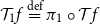 $\mathcal{T}_{1}{f}\stackrel {\mathrm{def}}= \pi_1\circ \mathcal{T}{f}$
and
$\mathcal{T}_{1}{f}\stackrel {\mathrm{def}}= \pi_1\circ \mathcal{T}{f}$
and
 $\mathcal{T}_{2}{f}\stackrel {\mathrm{def}}= \pi_2\circ \mathcal{T}{f}$
for the first and second components of
$\mathcal{T}_{2}{f}\stackrel {\mathrm{def}}= \pi_2\circ \mathcal{T}{f}$
for the first and second components of
 $\mathcal{T}{f}$
, respectively:
$\mathcal{T}{f}$
, respectively:
 $$\mathcal{T}\!\!{(g\circ f)}(x) = (\mathcal{T}_{1}{g}(\mathcal{T}_{1}{f}(x)),\mathcal{T}_{2}{g}(\mathcal{T}_{1}{f}(x))\circ \mathcal{T}_{2}{f}(x)).$$
We make two observations:
(1) the derivative of
 $g\circ f$
does depend not only on the derivatives of g and f but also on the primal value of f;
$g\circ f$
does depend not only on the derivatives of g and f but also on the primal value of f;
(2) the primal value of f is used twice: once in the primal value of
 $g\circ f $
and once in its derivative; we want to share these repeated subcomputations.
$g\circ f $
and once in its derivative; we want to share these repeated subcomputations.
Insight 1. This shows that it is wise to pair up computations of primal function values and derivatives and to share computation between both if we want to calculate derivatives of functions compositionally and efficiently.
Similar observations can be made for f’s transposed (adjoint) derivative
 ${Df}^{t}$
, which propagates not tangent vectors but cotangent vectors and which we can pair up as:
${Df}^{t}$
, which propagates not tangent vectors but cotangent vectors and which we can pair up as:
 \begin{align*}\mathcal{T}^*f : & \ {\mathbb{R}}^n \to {\mathbb{R}}^m\times (\underline{\mathbb{R}}^m\multimap \underline{\mathbb{R}}^n)\\ &x\mapsto (f(x),{Df}^{t}(x)) \end{align*}
to get the following chain rule:
 $$\mathcal{T}^*{(g\circ f)}(x) = (\mathcal{T}^*_{1}{g}(\mathcal{T}^*_{1}{f}(x)),\mathcal{T}^*_{2}{f}(x)\circ\mathcal{T}^*_{2}{g}(\mathcal{T}^*_{1}{f}(x))).$$
CHAD directly implements the operations
 $\mathcal{T}_{}$
and
$\mathcal{T}_{}$
and
 $\mathcal{T}^*$
as source code transformations
$\mathcal{T}^*$
as source code transformations
 $\overrightarrow{\mathcal{D}}$
and
$\overrightarrow{\mathcal{D}}$
and
 $\overleftarrow{\mathcal{D}}$
on a functional language to implement forward- and reverse-mode AD, respectively. These code transformations are defined compositionally through structural induction on the syntax, by making use of the chain rules above.
$\overleftarrow{\mathcal{D}}$
on a functional language to implement forward- and reverse-mode AD, respectively. These code transformations are defined compositionally through structural induction on the syntax, by making use of the chain rules above.
2.2 CHAD on a first-order functional language
We first discuss what the technique looks like on a standard typed first-order functional language. Despite our different presentation in terms of a
 $\lambda$
-calculus rather than Elliott’s categorical combinators, this is essentially the algorithm of Elliott (Reference Elliott2018). Types
$\lambda$
-calculus rather than Elliott’s categorical combinators, this is essentially the algorithm of Elliott (Reference Elliott2018). Types
 $\tau,\sigma,\rho$
are either statically sized arrays of n real numbers
$\tau,\sigma,\rho$
are either statically sized arrays of n real numbers
 ${\mathbf{real}}^n$
or tuples
${\mathbf{real}}^n$
or tuples
 $\tau\boldsymbol{\mathop{*}}\sigma$
of types
$\tau\boldsymbol{\mathop{*}}\sigma$
of types
 $\tau,\sigma$
. We consider programs t of type
$\tau,\sigma$
. We consider programs t of type
 $\sigma$
in typing context
$\sigma$
in typing context
 $\Gamma=x_1:\tau_1,\ldots,x_n:\tau_n$
, where
$\Gamma=x_1:\tau_1,\ldots,x_n:\tau_n$
, where
 $x_i$
are identifiers. We write such a typing judgment for programs in context as
$x_i$
are identifiers. We write such a typing judgment for programs in context as
 $\Gamma\vdash t:\sigma$
. As long as our language has certain primitive operations (which we represent schematically)
$\Gamma\vdash t:\sigma$
. As long as our language has certain primitive operations (which we represent schematically)
 $$\frac{\Gamma \vdash t_1 : {\mathbf{real}}^{n_1}\quad\cdots\quad \Gamma \vdash t_k : {\mathbf{real}}^{n_k}}{\Gamma \vdash \mathrm{op}(t_1,\ldots,t_k) : {\mathbf{real}}^m}$$
such as constants (as nullary operations), (elementwise) addition and multiplication of arrays, inner products and certain nonlinear functions like sigmoid functions, we can write complex programs by sequencing together such operations. For example, writing
 $\mathbf{real}$
for
$\mathbf{real}$
for
 ${\mathbf{real}}^1$
, we can write a program
${\mathbf{real}}^1$
, we can write a program
 $x_1:\mathbf{real},x_2:\mathbf{real},x_3:\mathbf{real},x_4:\mathbf{real}\vdash s:\mathbf{real}$
by:
$x_1:\mathbf{real},x_2:\mathbf{real},x_3:\mathbf{real},x_4:\mathbf{real}\vdash s:\mathbf{real}$
by:
 \begin{align*}&\mathbf{let}\,{y}=\,{x_1 * x_4 + 2 * x_2 }\,\mathbf{in}\,{}\\&\mathbf{let}\,{z}=\,{y* x_3}\,\mathbf{in}\,{}\\&\mathbf{let}\,w=\,{z+ x_4}\,\mathbf{in}\,{\sin{(w)}},\end{align*}
where we indicate shared subcomputations with
 $\mathbf{let}$
-bindings.
$\mathbf{let}$
-bindings.
CHAD observes that we can define for each language type
 $\tau$
associated types of
$\tau$
associated types of
-
• forward-mode primal values
$\overrightarrow{\mathcal{D}}(\tau)_{1}$
;

we define
 $\overrightarrow{\mathcal{D}}({\mathbf{real}}^n)={\mathbf{real}}^n$
and
$\overrightarrow{\mathcal{D}}({\mathbf{real}}^n)={\mathbf{real}}^n$
and
 $\overrightarrow{\mathcal{D}}(\tau\boldsymbol{\mathop{*}}\sigma)_1=\overrightarrow{\mathcal{D}}(\tau)_1\boldsymbol{\mathop{*}}\overrightarrow{\mathcal{D}}(\sigma)_1$
, that is, for now
$\overrightarrow{\mathcal{D}}(\tau\boldsymbol{\mathop{*}}\sigma)_1=\overrightarrow{\mathcal{D}}(\tau)_1\boldsymbol{\mathop{*}}\overrightarrow{\mathcal{D}}(\sigma)_1$
, that is, for now
 $\overrightarrow{\mathcal{D}}(\tau)_1=\tau$
;
$\overrightarrow{\mathcal{D}}(\tau)_1=\tau$
;
-
• reverse-mode primal values
$\overleftarrow{\mathcal{D}}(\tau)_1$
;

we define
 $\overleftarrow{\mathcal{D}}({\mathbf{real}}^n)={\mathbf{real}}^n$
and
$\overleftarrow{\mathcal{D}}({\mathbf{real}}^n)={\mathbf{real}}^n$
and
 $\overleftarrow{\mathcal{D}}(\tau)\boldsymbol{\mathop{*}}(\sigma)_1=\overleftarrow{\mathcal{D}}(\tau)_1\boldsymbol{\mathop{*}}\overleftarrow{\mathcal{D}}(\sigma)_1$
; that is, for now
$\overleftarrow{\mathcal{D}}(\tau)\boldsymbol{\mathop{*}}(\sigma)_1=\overleftarrow{\mathcal{D}}(\tau)_1\boldsymbol{\mathop{*}}\overleftarrow{\mathcal{D}}(\sigma)_1$
; that is, for now
 $\overleftarrow{\mathcal{D}}(\tau)_1=\tau$
;
$\overleftarrow{\mathcal{D}}(\tau)_1=\tau$
;
-
• forward-mode tangent values
$\overrightarrow{\mathcal{D}}(\tau)_2$
;

we define
 $\overrightarrow{\mathcal{D}}({\mathbf{real}}^n)_2=\underline{\mathbf{real}}^n$
and
$\overrightarrow{\mathcal{D}}({\mathbf{real}}^n)_2=\underline{\mathbf{real}}^n$
and
 $\overrightarrow{\mathcal{D}}(\tau\boldsymbol{\mathop{*}}\sigma)=\overrightarrow{\mathcal{D}}(\tau)_2\boldsymbol{\mathop{*}}\overrightarrow{\mathcal{D}}(\sigma)_2$
;
$\overrightarrow{\mathcal{D}}(\tau\boldsymbol{\mathop{*}}\sigma)=\overrightarrow{\mathcal{D}}(\tau)_2\boldsymbol{\mathop{*}}\overrightarrow{\mathcal{D}}(\sigma)_2$
;
-
• reverse-mode cotangent values
$\overleftarrow{\mathcal{D}}(\tau)_2$
;

we define
 $\overleftarrow{\mathcal{D}}({\mathbf{real}}^n)_2=\underline{\mathbf{real}}^n$
and
$\overleftarrow{\mathcal{D}}({\mathbf{real}}^n)_2=\underline{\mathbf{real}}^n$
and
 $\overleftarrow{\mathcal{D}}(\tau\boldsymbol{\mathop{*}}\sigma)=\overleftarrow{\mathcal{D}}(\tau)_2\boldsymbol{\mathop{*}}\overleftarrow{\mathcal{D}}(\sigma)_2$
.
$\overleftarrow{\mathcal{D}}(\tau\boldsymbol{\mathop{*}}\sigma)=\overleftarrow{\mathcal{D}}(\tau)_2\boldsymbol{\mathop{*}}\overleftarrow{\mathcal{D}}(\sigma)_2$
.
Indeed, the justification for these definitions is the crucial observation that a (co)tangent vector to a product of spaces is precisely a pair of tangent (co)vectors to the two spaces. Put differently, the space
 $\mathcal{T}_{(x,y)}{(X\times Y)}$
of (co)tangent vectors to
$\mathcal{T}_{(x,y)}{(X\times Y)}$
of (co)tangent vectors to
 $X\times Y$
at a point (x,y) equals the product space
$X\times Y$
at a point (x,y) equals the product space
 $(\mathcal{T}_{x}X) \times (\mathcal{T}_{y} Y)$
(Tu Reference Tu2011).
$(\mathcal{T}_{x}X) \times (\mathcal{T}_{y} Y)$
(Tu Reference Tu2011).
We write the (co)tangent types associated with
 ${\mathbf{real}}^n$
as
${\mathbf{real}}^n$
as
 $\underline{\mathbf{real}}^n$
to emphasize that it is a linear type and to distinguish it from the cartesian type
$\underline{\mathbf{real}}^n$
to emphasize that it is a linear type and to distinguish it from the cartesian type
 ${\mathbf{real}}^n$
. In particular, we will see that tangent and cotangent values are elements of linear types that come equipped with a commutative monoid structure
${\mathbf{real}}^n$
. In particular, we will see that tangent and cotangent values are elements of linear types that come equipped with a commutative monoid structure
 $(\underline{0},+)$
. Indeed, (transposed) derivatives are linear functions: homomorphisms of this monoid structure1. We extend these operations
$(\underline{0},+)$
. Indeed, (transposed) derivatives are linear functions: homomorphisms of this monoid structure1. We extend these operations
 $\overrightarrow{\mathcal{D}}$
and
$\overrightarrow{\mathcal{D}}$
and
 $\overleftarrow{\mathcal{D}}$
to act on typing contexts
$\overleftarrow{\mathcal{D}}$
to act on typing contexts
 $\Gamma$
:
$\Gamma$
:
 \begin{align*}\overrightarrow{\mathcal{D}}(x_1:\tau_1,\ldots,x_n:\tau_n)_1&=x_1:\overrightarrow{\mathcal{D}}(\tau_1)_1,\ldots, x_n:\overrightarrow{\mathcal{D}}(\tau_n)_1 \\\overleftarrow{\mathcal{D}}(x_1:\tau_1,\ldots,x_n:\tau_n)_1&=x_1:\overleftarrow{\mathcal{D}}(\tau_1)_1,\ldots, x_n:\overleftarrow{\mathcal{D}}(\tau_n)_1 \\\overrightarrow{\mathcal{D}}(x_1:\tau_1,\ldots,x_n:\tau_n)_2&=\overrightarrow{\mathcal{D}}(\tau_1)_2\boldsymbol{\mathop{*}}\cdots\boldsymbol{\mathop{*}}\overrightarrow{\mathcal{D}}(\tau_n)_2\\\overleftarrow{\mathcal{D}}(x_1:\tau_1,\ldots,x_n:\tau_n)_2&=\overleftarrow{\mathcal{D}}(\tau_1)_2\boldsymbol{\mathop{*}}\cdots\boldsymbol{\mathop{*}}\overleftarrow{\mathcal{D}}(\tau_n)_2.\end{align*}
To each program
 $\Gamma\vdash t:\sigma$
, CHAD associates programs calculating the forward-mode and reverse-mode derivatives
$\Gamma\vdash t:\sigma$
, CHAD associates programs calculating the forward-mode and reverse-mode derivatives
 $\overrightarrow{\mathcal{D}}_{{\overline{\Gamma}}}(t)$
and
$\overrightarrow{\mathcal{D}}_{{\overline{\Gamma}}}(t)$
and
 $\overleftarrow{\mathcal{D}}_{{\overline{\Gamma}}}(t)$
, which are indexed by the list
$\overleftarrow{\mathcal{D}}_{{\overline{\Gamma}}}(t)$
, which are indexed by the list
 ${\overline{\Gamma}}$
of identifiers that occur in
${\overline{\Gamma}}$
of identifiers that occur in
 $\Gamma$
:
$\Gamma$
:
 \begin{align*}&\overrightarrow{\mathcal{D}}(\Gamma)_1\vdash \overrightarrow{\mathcal{D}}_{\overline{\Gamma}}(t) : \overrightarrow{\mathcal{D}}(\sigma)(\boldsymbol){\mathop{*}} \left( \overrightarrow{\mathcal{D}}(\Gamma)_2\multimap \overrightarrow{\mathcal{D}}(\sigma)(\right)\\&\overleftarrow{\mathcal{D}}(\Gamma)_1\vdash \overleftarrow{\mathcal{D}}_{\overline{\Gamma}}(t) : \overleftarrow{\mathcal{D}}(\sigma)\boldsymbol{\mathop{*}} \left( \overleftarrow{\mathcal{D}}(\sigma)\multimap\overleftarrow{\mathcal{D}}(\Gamma)_2 \right).\end{align*}
Observing that each program t computes a differentiable function
 $\unicode{x27E6} t\unicode{x27E7}$
between Euclidean spaces, as long as all primitive operations op are differentiable, the key property that we prove for these code transformations is that they actually calculate derivatives:
$\unicode{x27E6} t\unicode{x27E7}$
between Euclidean spaces, as long as all primitive operations op are differentiable, the key property that we prove for these code transformations is that they actually calculate derivatives:
Theorem A (Correctness of CHAD, Theorem 124). For any well-typed program:
 $$x_1:{\mathbf{real}}^{n_1},\ldots,x_k:{\mathbf{real}}^{n_k}\vdash {t}:{\mathbf{real}}^m$$
we have that
 $\unicode{x27E6} \overrightarrow{\mathcal{D}}_{x_1,\ldots,x_k}(t)\unicode{x27E7}=\mathcal{T}_{\unicode{x27E6} t\unicode{x27E7}}\;\text{ and }\;\unicode{x27E6} \overleftarrow{\mathcal{D}}_{x_1,\ldots,x_k}(t)\unicode{x27E7}=\mathcal{T}^*{\unicode{x27E6} t\unicode{x27E7}}.$
Once we fix the semantics for the source and target languages, we can show that this theorem holds if we define
 $\overrightarrow{\mathcal{D}}$
and
$\overrightarrow{\mathcal{D}}$
and
 $\overleftarrow{\mathcal{D}}$
on programs using the chain rule. The proof works by plain induction on the syntax. For example, we can correctly define reverse-mode CHAD on a first-order language as follows:
$\overleftarrow{\mathcal{D}}$
on programs using the chain rule. The proof works by plain induction on the syntax. For example, we can correctly define reverse-mode CHAD on a first-order language as follows:
 \begin{align*} &\overleftarrow{\mathcal{D}}_{\overline{\Gamma}}(\mathrm{op}(t_1,\ldots,t_k)) \stackrel{\mathrm{def}}{=} && \mathbf{let}\,\langle x_1,x_1'\rangle=\,\overleftarrow{\mathcal{D}}_{\overline{\Gamma}}(t_1)\,\mathbf{in}\,\cdots\\ &&& \mathbf{let}\,\langle x_k,x_k'\rangle=\,\overleftarrow{\mathcal{D}}_{\overline{\Gamma}}(t_k)\,\mathbf{in}\,\\ &&&\langle\mathrm{op}(x_1,\ldots,x_k),\underline{\lambda} \mathsf{v}. \mathbf{let}\,\mathsf{v}=\,{D\mathrm{op}}^{t}(x_1,\ldots,x_k;\mathsf{v})\,\mathbf{in}\,\\ &&&\phantom{\langle \mathrm{op}(x_1,\ldots,x_k),\underline{\lambda} \mathsf{v}.\rangle}x_1'\bullet \mathbf{proj}_{1}\,{\mathsf{v}}+\cdots+x_k'\bullet \mathbf{proj}_{k}\,{\mathsf{v}}\rangle\end{align*}
 \begin{align*}&\overleftarrow{\mathcal{D}}_{\overline{\Gamma}}(x) \stackrel{\mathrm{def}}{=} && \langle x,\underline{\lambda} \mathsf{v}. \mathbf{coproj}_{\mathbf{idx}(x; {\overline{\Gamma}})\,}\,(\mathsf{v})\rangle\end{align*}
 \begin{align*} &\overleftarrow{\mathcal{D}}_{\overline{\Gamma}}(\mathbf{let}\,x=\,t\,\mathbf{in}\,s)\stackrel{\mathrm{def}}{=} &&\mathbf{let}\,\langle x,x'\rangle=\,\overleftarrow{\mathcal{D}}_{\overline{\Gamma}}(t)\,\mathbf{in}\,\\ &&& \mathbf{let}\,\langle y,y'\rangle=\,\overleftarrow{\mathcal{D}}_{\overline{\Gamma},x}(s)\,\mathbf{in}\,\\ &&& \langle y, \underline{\lambda} \mathsf{v}. \mathbf{let}\,\mathsf{v}=\,y'\bullet \mathsf{v}\,\mathbf{in}\, \mathbf{fst}\,\mathsf{v}+x'\bullet (\mathbf{snd}\, \mathsf{v})\rangle\end{align*}
 \begin{align*}&\overleftarrow{\mathcal{D}}_{\overline{\Gamma}}(\langle t, s\rangle) \stackrel {\mathrm{def}}= &&\mathbf{let}\,\langle x,x'\rangle=\,\overleftarrow{\mathcal{D}}_{\overline{\Gamma}}(t)\,\mathbf{in}\, \\ &&&\mathbf{let}\,\langle y,y'\rangle=\,\overleftarrow{\mathcal{D}}_{\overline{\Gamma}}(s)\,\mathbf{in}\,\\ &&&\langle \langle x, y \rangle,\underline{\lambda} \mathsf{v}. x'\bullet (\mathbf{fst}\,\mathsf{v}) + {y'\bullet(\mathbf{snd}\, \mathsf{v})}\rangle\end{align*}
 \begin{align*}&\overleftarrow{\mathcal{D}}_{\overline{\Gamma}}(\mathbf{fst}\, t) \stackrel {\mathrm{def}}= &&\mathbf{let}\,\langle x,x'\rangle=\,\overleftarrow{\mathcal{D}}_{\overline{\Gamma}}(t)\,\mathbf{in}\,\langle \mathbf{fst}\, x, \underline{\lambda} \mathsf{v}. x'\bullet \langle\mathsf{v},\underline{0}\rangle\rangle\end{align*}
 \begin{align*}&\overleftarrow{\mathcal{D}}_{\overline{\Gamma}}(\mathbf{snd}\, t) \stackrel {\mathrm{def}}= &&\mathbf{let}\,\langle x,x'\rangle=\,\overleftarrow{\mathcal{D}}_{\overline{\Gamma}}(t)\,\mathbf{in}\,\langle\mathbf{snd}\, x,\underline{\lambda} \mathsf{v}. x'\bullet\langle\underline{0},\mathsf{v}\rangle\rangle\end{align*}
Here, we write
 $\underline{\lambda} \mathsf{v}. t$
for a linear function abstraction (merely a notational convention – it can simply be thought of as a plain function abstraction) and
$\underline{\lambda} \mathsf{v}. t$
for a linear function abstraction (merely a notational convention – it can simply be thought of as a plain function abstraction) and
 $t\bullet s$
for a linear function application (which again can be thought of as a plain function application). Furthermore, given
$t\bullet s$
for a linear function application (which again can be thought of as a plain function application). Furthermore, given
 $\Gamma;\mathsf{v}:\underline{\alpha}\vdash t:\boldsymbol{(}\underline{\sigma}_1 \boldsymbol{\mathop{*}} \cdots \boldsymbol{\mathop{*}} \underline{\sigma}_n\boldsymbol{)}$
, we write
$\Gamma;\mathsf{v}:\underline{\alpha}\vdash t:\boldsymbol{(}\underline{\sigma}_1 \boldsymbol{\mathop{*}} \cdots \boldsymbol{\mathop{*}} \underline{\sigma}_n\boldsymbol{)}$
, we write
 $\Gamma;\mathsf{v}:\underline{\alpha}\vdash \mathbf{proj}_{i}\,(t):\underline{\sigma}_i$
for the i-th projection of t. Similarly, given
$\Gamma;\mathsf{v}:\underline{\alpha}\vdash \mathbf{proj}_{i}\,(t):\underline{\sigma}_i$
for the i-th projection of t. Similarly, given
 $\Gamma;\mathsf{v}:\underline{\alpha}\vdash t:\underline{\sigma}_i$
, we write the i-th coprojection
$\Gamma;\mathsf{v}:\underline{\alpha}\vdash t:\underline{\sigma}_i$
, we write the i-th coprojection
 $\Gamma;\mathsf{v}:\underline{\alpha}\vdash\mathbf{coproj}_{i}\,(t)= \langle \underline{0},\ldots,\underline{0},t,\underline{0},\ldots,\underline{0}\rangle:\boldsymbol{(}\underline{\sigma}_1 \boldsymbol{\mathop{*}} \cdots \boldsymbol{\mathop{*}} \underline{\alpha}_n\boldsymbol{)}$
and we write
$\Gamma;\mathsf{v}:\underline{\alpha}\vdash\mathbf{coproj}_{i}\,(t)= \langle \underline{0},\ldots,\underline{0},t,\underline{0},\ldots,\underline{0}\rangle:\boldsymbol{(}\underline{\sigma}_1 \boldsymbol{\mathop{*}} \cdots \boldsymbol{\mathop{*}} \underline{\alpha}_n\boldsymbol{)}$
and we write
 $\mathbf{idx}(x_i; x_1,\ldots,x_n)\,=i$
for the index of an identifier in a list of identifiers. Finally,
$\mathbf{idx}(x_i; x_1,\ldots,x_n)\,=i$
for the index of an identifier in a list of identifiers. Finally,
 ${D\mathrm{op}}^{t}$
here is a linear operation that implements the transposed derivative of the primitive operation op.
${D\mathrm{op}}^{t}$
here is a linear operation that implements the transposed derivative of the primitive operation op.
Note, in particular, that CHAD pairs up primal and (co)tangent values and shares common subcomputations. We see that what CHAD achieves is a compositional efficient reverse-mode AD algorithm that computes the (transposed) derivatives of a composite program in terms of the (transposed) derivatives
 ${D\mathrm{op}}^{t}$
of the basic building blocks op.
${D\mathrm{op}}^{t}$
of the basic building blocks op.
2.3 CHAD on a higher-order language: a categorical perspective saves the day
So far, this account of CHAD has been smooth sailing: we can simply follow the usual mathematics of (transposed) derivatives of functions
 ${\mathbb{R}}^n\to {\mathbb{R}}^m$
and implement it in code. A challenge arises when trying to extend the algorithm to more expressive languages with features that do not have an obvious counterpart in multivariate calculus, like higher-order functions.
${\mathbb{R}}^n\to {\mathbb{R}}^m$
and implement it in code. A challenge arises when trying to extend the algorithm to more expressive languages with features that do not have an obvious counterpart in multivariate calculus, like higher-order functions.
Vákár and Smeding (Reference Vákár and Smeding2022) and Vákár (Reference Vákár2021) solve this problem by observing that we can understand CHAD through the categorical structure of Grothendieck constructions (aka
 $\Sigma$
-types of categories). In particular, they observe that the syntactic category of the target language for CHAD, a language with both cartesian and linear types, forms a locally indexed category
$\Sigma$
-types of categories). In particular, they observe that the syntactic category of the target language for CHAD, a language with both cartesian and linear types, forms a locally indexed category
 ${\mathbf{LSyn}}:{\mathbf{CSyn}}^{op}\to \mathbf{Cat}$
, that is, functor to the category of categories and functors for which
${\mathbf{LSyn}}:{\mathbf{CSyn}}^{op}\to \mathbf{Cat}$
, that is, functor to the category of categories and functors for which
 $\mathrm{obj} \left( {\mathbf{LSyn}}\right)(\tau)=\mathrm{obj} \left( {\mathbf{LSyn}}\right)(\sigma)$
for all
$\mathrm{obj} \left( {\mathbf{LSyn}}\right)(\tau)=\mathrm{obj} \left( {\mathbf{LSyn}}\right)(\sigma)$
for all
 $\tau,\sigma\in\mathrm{obj} \left( {\mathbf{CSyn}}\right)$
and
$\tau,\sigma\in\mathrm{obj} \left( {\mathbf{CSyn}}\right)$
and
 ${\mathbf{LSyn}}(\tau\xrightarrow{t}\sigma):{\mathbf{LSyn}}(\sigma)\to{\mathbf{LSyn}}(\tau)$
is identity on objects. Here,
${\mathbf{LSyn}}(\tau\xrightarrow{t}\sigma):{\mathbf{LSyn}}(\sigma)\to{\mathbf{LSyn}}(\tau)$
is identity on objects. Here,
 ${\mathbf{CSyn}} $
is the syntactic category whose objects are cartesian types
${\mathbf{CSyn}} $
is the syntactic category whose objects are cartesian types
 $\tau,\sigma,\rho$
and morphisms
$\tau,\sigma,\rho$
and morphisms
 $\tau\to \sigma$
are programs
$\tau\to \sigma$
are programs
 $x:\tau\vdash t:\sigma$
, up to a standard program equivalence. Similarly,
$x:\tau\vdash t:\sigma$
, up to a standard program equivalence. Similarly,
 ${\mathbf{LSyn}}(\tau)$
is the syntactic category whose objects are linear types
${\mathbf{LSyn}}(\tau)$
is the syntactic category whose objects are linear types
 $\underline{\alpha},\underline{\sigma},\underline{\gamma}$
and morphisms
$\underline{\alpha},\underline{\sigma},\underline{\gamma}$
and morphisms
 $\underline{\alpha}\to\underline{\gamma}$
are programs
$\underline{\alpha}\to\underline{\gamma}$
are programs
 $x:\tau;\mathsf{v}:\underline{\alpha}\vdash t:\underline{\gamma}$
of type
$x:\tau;\mathsf{v}:\underline{\alpha}\vdash t:\underline{\gamma}$
of type
 $\underline{\gamma}$
that have a free variable x of cartesian type
$\underline{\gamma}$
that have a free variable x of cartesian type
 $\tau$
and a free variable
$\tau$
and a free variable
 $\mathsf{v}$
of linear type
$\mathsf{v}$
of linear type
 $\underline{\alpha}$
. The key observation then is the following.
$\underline{\alpha}$
. The key observation then is the following.
Theorem B (CHAD from a universal property, Corollary 69). Forward- and reverse-mode CHAD are the unique structure-preserving functors:
 \begin{align*} &\overrightarrow{\mathcal{D}}({-}):\mathbf{Syn}\to \Sigma_{{\mathbf{CSyn}}}{\mathbf{LSyn}}\\ &\overleftarrow{\mathcal{D}}({-}):\mathbf{Syn}\to \Sigma_{{\mathbf{CSyn}}}{\mathbf{LSyn}}^{op}\end{align*}
from the syntactic category
 $\mathbf{Syn}$
of the source language to (opposite) Grothendieck construction of the target language
$\mathbf{Syn}$
of the source language to (opposite) Grothendieck construction of the target language
 ${\mathbf{LSyn}}:{\mathbf{CSyn}}^{op}\to \mathbf{Cat}$
that send primitive operations op to their derivative
${\mathbf{LSyn}}:{\mathbf{CSyn}}^{op}\to \mathbf{Cat}$
that send primitive operations op to their derivative
 $D\mathrm{op}$
and transposed derivative
$D\mathrm{op}$
and transposed derivative
 ${D\mathrm{op}}^{t}$
, respectively.
${D\mathrm{op}}^{t}$
, respectively.
In particular, they prove that this is true for the unambiguous definitions of CHAD for a source language that is the first-order functional language we have considered above, which we can see as the freely generated category
 $\mathbf{Syn}$
with finite products, generated by the objects
$\mathbf{Syn}$
with finite products, generated by the objects
 ${\mathbf{real}}^n$
and morphisms op. That is, for this limited language, “structure-preserving functor” should be interpreted as “finite product-preserving functor.”
${\mathbf{real}}^n$
and morphisms op. That is, for this limited language, “structure-preserving functor” should be interpreted as “finite product-preserving functor.”
This leads (Vákár Reference Vákár2021; Vákár and Smeding Reference Vákár and Smeding2022) to the idea to try to use Theorem B as a definition of CHAD on more expressive programming languages. In particular, they consider a higher-order functional source language
 $\mathbf{Syn}$
, that is, the freely generated cartesian closed category on the objects
$\mathbf{Syn}$
, that is, the freely generated cartesian closed category on the objects
 ${\mathbf{real}}^n$
and morphisms op and try to define
${\mathbf{real}}^n$
and morphisms op and try to define
 $\overrightarrow{\mathcal{D}}(-)$
and
$\overrightarrow{\mathcal{D}}(-)$
and
 $\overleftarrow{\mathcal{D}}(-)$
as the (unique) structure-preserving (meaning: cartesian closed) functors to
$\overleftarrow{\mathcal{D}}(-)$
as the (unique) structure-preserving (meaning: cartesian closed) functors to
 $\Sigma_{{\mathbf{CSyn}}}{\mathbf{LSyn}}$
and
$\Sigma_{{\mathbf{CSyn}}}{\mathbf{LSyn}}$
and
 $\Sigma_{{\mathbf{CSyn}}}{\mathbf{LSyn}}^{op}$
for a suitable linear target language
$\Sigma_{{\mathbf{CSyn}}}{\mathbf{LSyn}}^{op}$
for a suitable linear target language
 ${\mathbf{LSyn}}:{\mathbf{CSyn}}^{op}\to \mathbf{Cat}$
. The main contribution then is to identify conditions on a locally indexed category
${\mathbf{LSyn}}:{\mathbf{CSyn}}^{op}\to \mathbf{Cat}$
. The main contribution then is to identify conditions on a locally indexed category
 $\mathcal{L}:\mathcal{C}^{op}\to \mathbf{Cat}$
that guarantee that
$\mathcal{L}:\mathcal{C}^{op}\to \mathbf{Cat}$
that guarantee that
 $\Sigma_{\mathcal{C}}\mathcal{L}$
and
$\Sigma_{\mathcal{C}}\mathcal{L}$
and
 $\Sigma_{\mathcal{C}}\mathcal{L}^{op}$
are cartesian closed and to take the target language
$\Sigma_{\mathcal{C}}\mathcal{L}^{op}$
are cartesian closed and to take the target language
 ${\mathbf{LSyn}}:{\mathbf{CSyn}}^{op}\to \mathbf{Cat}$
as a freely generated such category.
${\mathbf{LSyn}}:{\mathbf{CSyn}}^{op}\to \mathbf{Cat}$
as a freely generated such category.
Insight 2. To understand how to perform CHAD on a source language with language feature X (e.g., higher-order functions), we need to understand the categorical semantics of language feature X (e.g., categorical exponentials) in categories of the form
 $\Sigma_\mathcal{C}\mathcal{L}$
and
$\Sigma_\mathcal{C}\mathcal{L}$
and
 $\Sigma_\mathcal{C}\mathcal{L}^{op}$
. Giving sufficient conditions on
$\Sigma_\mathcal{C}\mathcal{L}^{op}$
. Giving sufficient conditions on
 $\mathcal{L}$
for such a semantics to exist yields a suitable target language for CHAD, with the definition of the algorithm falling from the universal property of the source language.
$\mathcal{L}$
for such a semantics to exist yields a suitable target language for CHAD, with the definition of the algorithm falling from the universal property of the source language.
Furthermore, we observe in these papers that Theorem A again holds for this extended definition of CHAD on higher-order languages. However, to prove this, plain induction no longer suffices and we instead need to use a logical relations construction over the semantics (in the form of categorical sconing) that relates differentiable curves to their associated primal and (co)tangent curves. This is necessary because the program t may use higher-order constructions such as
 $\lambda$
-abstractions and function applications in its definition, even if the input and output types are plain first-order types that implement some Euclidean space.
$\lambda$
-abstractions and function applications in its definition, even if the input and output types are plain first-order types that implement some Euclidean space.
Insight 3. To obtain a correctness proof of CHAD on source languages with language feature X, it suffices to give a concrete denotational semantics for the source and target languages as well as a categorical semantics of language feature X in a category of logical relations (a scone) over these concrete semantics. The main technical challenge is to analyze logical relations techniques for language feature X.
Finally, these papers observe that the resulting target language can be implemented as a shallowly embedded DSL in standard functional languages, using a module system to implement the required linear types as abstract types, with a reference Haskell implementation available at https://github.com/VMatthijs/CHAD. In fact, Vytiniotis et al. (Reference Vytiniotis, Belov, Wei, Plotkin and Abadi2019) had proposed the same CHAD algorithm for higher-order languages, arriving at it from practical considerations rather than abstract categorical observations.
Insight 4. The code generated by CHAD naturally comes equipped with very precise (e.g., linear) types. These types emphasize the connections to its mathematical foundations and provide scaffolding for its correctness proof. However, they are unnecessary for a practical implementation of the algorithm: CHAD can be made to generate standard functional (e.g., Haskell) code; the type safety can even be rescued by implementing the linear types as abstract types.
2.4 CHAD for sum types: a challenge – (co)tangent spaces of varying dimension
A natural approach, therefore, when extending CHAD to yet more expressive source languages is to try to use Theorem B as a definition. In the case of sum types (aka variant types), therefore, we should consider their categorical equivalent, distributive coproducts, and seek conditions on
 $\mathcal{L}:\mathcal{C}^{op}\to\mathbf{Cat}$
under which
$\mathcal{L}:\mathcal{C}^{op}\to\mathbf{Cat}$
under which
 $\Sigma_{\mathcal{C}}\mathcal{L}$
and
$\Sigma_{\mathcal{C}}\mathcal{L}$
and
 $\Sigma_{\mathcal{C}}\mathcal{L}^{op}$
have distributive coproducts. The difficulty is that these categories tend not to have coproducts if
$\Sigma_{\mathcal{C}}\mathcal{L}^{op}$
have distributive coproducts. The difficulty is that these categories tend not to have coproducts if
 $\mathcal{L}$
is locally indexed. Instead, the desire to have coproducts in
$\mathcal{L}$
is locally indexed. Instead, the desire to have coproducts in
 $\Sigma_{\mathcal{C}}\mathcal{L}$
and
$\Sigma_{\mathcal{C}}\mathcal{L}$
and
 $\Sigma_{\mathcal{C}}\mathcal{L}^{op}$
naturally leads us to consider more general strictly indexed categories
$\Sigma_{\mathcal{C}}\mathcal{L}^{op}$
naturally leads us to consider more general strictly indexed categories
 $\mathcal{L}:\mathcal{C}^{op}\to\mathbf{Cat}$
.
$\mathcal{L}:\mathcal{C}^{op}\to\mathbf{Cat}$
.
In fact, this is compatible with what we know from differential geometry (Tu Reference Tu2011): coproducts allow us to construct spaces with multiple connected components, each of which may have a distinct dimension. To make things concrete, the space
 $\mathcal{T}_{x}{({\mathbb{R}}^2 \sqcup {\mathbb{R}}^3)}$
of tangent vectors to
$\mathcal{T}_{x}{({\mathbb{R}}^2 \sqcup {\mathbb{R}}^3)}$
of tangent vectors to
 ${\mathbb{R}}^2 \sqcup {\mathbb{R}}^3$
is either
${\mathbb{R}}^2 \sqcup {\mathbb{R}}^3$
is either
 $\underline{\mathbb{R}}^2$
or
$\underline{\mathbb{R}}^2$
or
 $\underline{\mathbb{R}}^3$
depending on whether the base point x is chosen in the left or right component of the coproduct. More generally, a differentiable function
$\underline{\mathbb{R}}^3$
depending on whether the base point x is chosen in the left or right component of the coproduct. More generally, a differentiable function
 $f:X\to Y$
between spaces of varying dimension (which can be formalized as manifolds with multiple connected components) induces functions on the spaces of tangent and cotangent vectors2:
$f:X\to Y$
between spaces of varying dimension (which can be formalized as manifolds with multiple connected components) induces functions on the spaces of tangent and cotangent vectors2:
 \begin{align*}\mathcal{T}{f}&:\Pi_{x\in X}\Sigma_{y\in Y}(\mathcal{T}_{x} X\multimap \mathcal{T}_{y}Y)\\\mathcal{T}^*{f}&:\Pi_{x\in X}\Sigma_{y\in Y}(\mathcal{T}^*_{y} Y\multimap \mathcal{T}^*_{x}X),\end{align*}
whose first component is f itself and whose second component is the action on (co)tangent vectors that f induces.
If the types
 $\overrightarrow{\mathcal{D}}(\tau)_2$
and
$\overrightarrow{\mathcal{D}}(\tau)_2$
and
 $\overleftarrow{\mathcal{D}}(\tau)_2$
are to represent spaces of tangent and cotangent vectors to the spaces that
$\overleftarrow{\mathcal{D}}(\tau)_2$
are to represent spaces of tangent and cotangent vectors to the spaces that
 $\overrightarrow{\mathcal{D}}(\tau)_{1}$
and
$\overrightarrow{\mathcal{D}}(\tau)_{1}$
and
 $\overleftarrow{\mathcal{D}}(\tau)_1$
represent, we would expect them to be types that vary with the particular base point (primal) we choose. This leads to a refined view of CHAD: while
$\overleftarrow{\mathcal{D}}(\tau)_1$
represent, we would expect them to be types that vary with the particular base point (primal) we choose. This leads to a refined view of CHAD: while
 $\vdash \overrightarrow{\mathcal{D}}(\tau)_1:\mathrm{type} $
and
$\vdash \overrightarrow{\mathcal{D}}(\tau)_1:\mathrm{type} $
and
 $\vdash\overleftarrow{\mathcal{D}}(\tau)_1:\mathrm{type}$
can remain (closed/nondependent) cartesian types,
$\vdash\overleftarrow{\mathcal{D}}(\tau)_1:\mathrm{type}$
can remain (closed/nondependent) cartesian types,
 ${p}:\overrightarrow{\mathcal{D}}(\tau)_1\vdash \overrightarrow{\mathcal{D}}(\tau)_2:\mathrm{ltype}$
and
${p}:\overrightarrow{\mathcal{D}}(\tau)_1\vdash \overrightarrow{\mathcal{D}}(\tau)_2:\mathrm{ltype}$
and
 ${p}:\overleftarrow{\mathcal{D}}(\tau)_1\vdash \overleftarrow{\mathcal{D}}(\tau)_2:\mathrm{ltype}$
are, in general, linear dependent types.
${p}:\overleftarrow{\mathcal{D}}(\tau)_1\vdash \overleftarrow{\mathcal{D}}(\tau)_2:\mathrm{ltype}$
are, in general, linear dependent types.
Insight 5. To accommodate sum types in CHAD, it is natural to consider a target language with dependent types: this allows the dimension of the spaces of (co)tangent vectors to vary with the chosen primal. In categorical terms, we need to consider general strictly indexed categories
 $\mathcal{L}:\mathcal{C}^{op}\to \mathbf{Cat}$
instead of merely locally indexed ones.
$\mathcal{L}:\mathcal{C}^{op}\to \mathbf{Cat}$
instead of merely locally indexed ones.
The CHAD transformations of the program now becomes typed in the following more precise way:
 \[\begin{array}{l} \overrightarrow{\mathcal{D}}(\Gamma)_1\vdash \overrightarrow{\mathcal{D}}_{\overline{\Gamma}}(t):\Sigma{{p}:\overrightarrow{\mathcal{D}}(\tau)_1}.{\overrightarrow{\mathcal{D}}(\Gamma)_2\multimap \overrightarrow{\mathcal{D}}(\tau)_2}\\ \overleftarrow{\mathcal{D}}(\Gamma)_1\vdash \overleftarrow{\mathcal{D}}_{\overline{\Gamma}}(t):\Sigma{{p}:\overleftarrow{\mathcal{D}}(\tau)_1}.{\overleftarrow{\mathcal{D}}(\tau)_2\multimap \overleftarrow{\mathcal{D}}(\Gamma)_2},\end{array}\]
where the action of
 $\overrightarrow{\mathcal{D}}({-})_2$
and
$\overrightarrow{\mathcal{D}}({-})_2$
and
 $\overleftarrow{\mathcal{D}}(-)_2$
on typing contexts
$\overleftarrow{\mathcal{D}}(-)_2$
on typing contexts
 $\Gamma=x_1:\tau_1,\ldots,x_n:\tau_n$
has been refined to
$\Gamma=x_1:\tau_1,\ldots,x_n:\tau_n$
has been refined to
 \[ \overrightarrow{\mathcal{D}}(\Gamma)_2\stackrel {\mathrm{def}}= \boldsymbol{(}\overrightarrow{\mathcal{D}}\tau_1)_2[{}^{x_1}\!/\!_{{p}}] \boldsymbol{\mathop{*}} \cdots \boldsymbol{\mathop{*}} \overrightarrow{\mathcal{D}}\tau_n)_2[{}^{x_n}\!/\!_{{p}}]\boldsymbol{)}\qquad\quad \overleftarrow{\mathcal{D}}(\Gamma)_2\stackrel {\mathrm{def}}= \boldsymbol{(}\overleftarrow{\mathcal{D}}(\tau_1)_2[{}^{x_1}\!/\!_{{p}}] \boldsymbol{\mathop{*}} \cdots \boldsymbol{\mathop{*}} \overleftarrow{\mathcal{D}}(\tau_n)_2[{}^{x_n}\!/\!_{{p}}]\boldsymbol{)}.\]
All given definitions remain valid, where we simply reinterpret some tuples as having a
 $\Sigma$
-type rather than the more limited original tuple type.
$\Sigma$
-type rather than the more limited original tuple type.
We prove the following novel results.
Theorem C (Bicartesian closed structure of
 $\Sigma$
-categories, Propositions 17 and 18, Theorems 25, 26, and 39, and Corollaries 35 and 36). For a category
$\Sigma$
-categories, Propositions 17 and 18, Theorems 25, 26, and 39, and Corollaries 35 and 36). For a category
 $\mathcal{C}$
and a strictly indexed category
$\mathcal{C}$
and a strictly indexed category
 $\mathcal{L}:\mathcal{C}^{op}\to \mathbf{Cat}$
,
$\mathcal{L}:\mathcal{C}^{op}\to \mathbf{Cat}$
,
 $\Sigma_\mathcal{C} \mathcal{L}$
and
$\Sigma_\mathcal{C} \mathcal{L}$
and
 $\Sigma_\mathcal{C} \mathcal{L}^{op}$
have
$\Sigma_\mathcal{C} \mathcal{L}^{op}$
have
-
• (fibered) finite products, if
$\mathcal{C}$
has finite coproducts and
$\mathcal{L}$
has strictly indexed products and coproducts; -
• (fibered) finite coproducts, if
$\mathcal{C}$
has finite coproducts and
$\mathcal{L}$
is extensive; -
• exponentials, if
$\mathcal{L}$
is a biadditive model of the dependently typed enriched effect calculus (we intentially keep this vague here to aid legibility – the point is that these are relatively standard conditions).


Furthermore, the coproducts in
 $\Sigma_\mathcal{C} \mathcal{L}$
and
$\Sigma_\mathcal{C} \mathcal{L}$
and
 $\Sigma_\mathcal{C} \mathcal{L}^{op}$
distribute over the products, as long as those in
$\Sigma_\mathcal{C} \mathcal{L}^{op}$
distribute over the products, as long as those in
 $\mathcal{C}$
do, even in the absence of exponentials. Notably, the exponentials are not generally fibered over
$\mathcal{C}$
do, even in the absence of exponentials. Notably, the exponentials are not generally fibered over
 $\mathcal{C}$
.
$\mathcal{C}$
.
The crucial notion here is our (novel) notion of extensivity of an indexed category, which generalizes well-known notions of extensive categories. In particular, we call
 $\mathcal{L}:\mathcal{C}^{op}\to \mathbf{Cat}$
extensive if the canonical functor
$\mathcal{L}:\mathcal{C}^{op}\to \mathbf{Cat}$
extensive if the canonical functor
 $\mathcal{L}(\sqcup_{i=1}^n C_i)\to \prod_{i=1}^n \mathcal{L}(C_i)$
is an equivalence. Furthermore, we note that we need to reestablish the product and exponential structures of
$\mathcal{L}(\sqcup_{i=1}^n C_i)\to \prod_{i=1}^n \mathcal{L}(C_i)$
is an equivalence. Furthermore, we note that we need to reestablish the product and exponential structures of
 $\Sigma_\mathcal{C} \mathcal{L}$
and
$\Sigma_\mathcal{C} \mathcal{L}$
and
 $\Sigma_\mathcal{C} \mathcal{L}^{op}$
due to the generalization from locally indexed to arbitrary strictly indexed categories
$\Sigma_\mathcal{C} \mathcal{L}^{op}$
due to the generalization from locally indexed to arbitrary strictly indexed categories
 $\mathcal{L}$
.
$\mathcal{L}$
.
Using these results, we construct a suitable target language
 ${\mathbf{LSyn}}:{\mathbf{CSyn}}^{op}\to\mathbf{Cat}$
for CHAD on a source language with sum types (and tuple and function types) and derive the forward and reverse CHAD algorithms for such a language and reestablish Theorems A and B in this more general context. This target language is a standard dependently typed enriched effect calculus with cartesian sum types and extensive families of linear types (i.e., dependent linear types that can be defined through case distinction). Again, the correctness proof of Theorem A uses the universal property of Theorem B and a logical relations (categorical sconing) construction over the denotational semantics of the source and target languages. This logical relations construction is relatively straightforward and relies on well-known sconing methods for bicartesian closed categories. In particular, we obtain the following formulas for a sum type
${\mathbf{LSyn}}:{\mathbf{CSyn}}^{op}\to\mathbf{Cat}$
for CHAD on a source language with sum types (and tuple and function types) and derive the forward and reverse CHAD algorithms for such a language and reestablish Theorems A and B in this more general context. This target language is a standard dependently typed enriched effect calculus with cartesian sum types and extensive families of linear types (i.e., dependent linear types that can be defined through case distinction). Again, the correctness proof of Theorem A uses the universal property of Theorem B and a logical relations (categorical sconing) construction over the denotational semantics of the source and target languages. This logical relations construction is relatively straightforward and relies on well-known sconing methods for bicartesian closed categories. In particular, we obtain the following formulas for a sum type
 $\left\{\ell_1\tau_1\mid\cdots\mid \ell_n\tau_n\right\}$
with constructors
$\left\{\ell_1\tau_1\mid\cdots\mid \ell_n\tau_n\right\}$
with constructors
 $\ell_1,\ldots,\ell_n$
that take arguments of type
$\ell_1,\ldots,\ell_n$
that take arguments of type
 $\tau_1,\ldots,\tau_n$
:
$\tau_1,\ldots,\tau_n$
:
 \begin{align*} &\overrightarrow{\mathcal{D}}\left\{\ell_1\tau_1\mid\cdots\mid \ell_n\tau_n\right\})_1 \stackrel {\mathrm{def}}= \left\{\ell_1\overrightarrow{\mathcal{D}}\tau_1)_1\mid \cdots \mid\ell_n\overrightarrow{\mathcal{D}}\tau_n)_1\right\}\\ &\overrightarrow{\mathcal{D}}\left\{\ell_1\tau_1\mid\cdots\mid \ell_n\tau_n\right\})_2\stackrel {\mathrm{def}}= {\mathbf{case}\,{p}\,\mathbf{of}\,\{{\ell_1{p}\to \overrightarrow{\mathcal{D}}\tau_1)_2\mid\cdots\mid \ell_n{p}\to\overrightarrow{\mathcal{D}}\tau_n)_2}\}}\\ &\overleftarrow{\mathcal{D}}(\left\{\ell_1\tau_1\mid\cdots\mid \ell_n\tau_n\right\})_1 \stackrel {\mathrm{def}}= \left\{\ell_1\overleftarrow{\mathcal{D}}(\tau_1)_1\mid \cdots \mid\ell_n\overleftarrow{\mathcal{D}}(\tau_n)_1\right\}\\ &\overleftarrow{\mathcal{D}}(\left\{\ell_1\tau_1\mid\cdots\mid \ell_n\tau_n\right\})_2\stackrel {\mathrm{def}}= {\mathbf{case}\,{p}\,\mathbf{of}\,\{{\ell_1{p}\to \overrightarrow{\mathcal{D}}\tau_1)_2\mid\cdots\mid \ell_n{p}\to\overleftarrow{\mathcal{D}}(\tau_n)_2}\}},\end{align*}
mirroring our intuition that the (co)tangent bundle to a coproduct of spaces decomposes (extensively) into the (co)tangent bundles to the component spaces.
2.5 CHAD for (co)inductive types: where do we begin?
If we are to really push forward the dream of differentiable programming, we need to learn how to perform AD on programs that operate on data types. To this effect, we analyze CHAD for inductive and coinductive types. If we want to follow our previous methodology to find suitable definitions and correctness proofs, we first need a good categorical axiomatization of such types. It is well known that inductive types correspond to initial algebras of functors, while coinductive types are precisely terminal coalgebras. The question, however, is what class of functors to consider. That choice makes the vague notion of (co)inductive types precise.
Following Santocanale (Reference Santocanale2002), we work with the class of
 $\mu\nu$
-polynomials, a relatively standard choice, that is functors that can be defined inductively through the combination of
$\mu\nu$
-polynomials, a relatively standard choice, that is functors that can be defined inductively through the combination of
-
• constants for primitive types
${\mathbf{real}}^n$
; -
• type variables
${\alpha}$
; -
• unit and tuple types
$\mathbf{1}$
and
$\tau\boldsymbol{\mathop{*}}\sigma$
of
$\mu\nu$
-polynomials; -
• sum types
$\left\{\ell_1\tau_1\mid\cdots\mid \ell_n\tau_n\right\}$
of
$\mu\nu$
-polynomials; -
• initial algebras
$\mu{\alpha}.\tau$
of
$\mu\nu$
-polynomials; -
• terminal coalgebras
$\nu{\alpha}.\tau$
of
$\mu\nu$
-polynomials.


Notably, we exclude function types, as the non-fibered nature of exponentials in
 $\Sigma_\mathcal{C} \mathcal{L}$
and
$\Sigma_\mathcal{C} \mathcal{L}$
and
 $\Sigma_\mathcal{C} \mathcal{L}^{op}$
would significantly complicate the technical development. While this excludes certain examples like the free state monad (which for type
$\Sigma_\mathcal{C} \mathcal{L}^{op}$
would significantly complicate the technical development. While this excludes certain examples like the free state monad (which for type
 $\sigma$
state would be the intial algebra
$\sigma$
state would be the intial algebra
 $\mu{\alpha}.\left\{Get (\sigma\to {\alpha})\mid Put (\sigma\boldsymbol{\mathop{*}} {\alpha})\right\}$
), it still includes the vast majority of examples of eager and lazy types that one uses in practice, for example, lists
$\mu{\alpha}.\left\{Get (\sigma\to {\alpha})\mid Put (\sigma\boldsymbol{\mathop{*}} {\alpha})\right\}$
), it still includes the vast majority of examples of eager and lazy types that one uses in practice, for example, lists
 $\mu{\alpha}.\left\{Empty\,\mathbf{1}\mid Cons (\sigma\boldsymbol{\mathop{*}} {\alpha})\right\}$
, (finitely branching) labeled trees like
$\mu{\alpha}.\left\{Empty\,\mathbf{1}\mid Cons (\sigma\boldsymbol{\mathop{*}} {\alpha})\right\}$
, (finitely branching) labeled trees like
 $\mu{\alpha}.\left\{Leaf\,\mathbf{1}\mid Node (\sigma\boldsymbol{\mathop{*}} {\alpha}\boldsymbol{\mathop{*}} {\alpha})\right\}$
, streams
$\mu{\alpha}.\left\{Leaf\,\mathbf{1}\mid Node (\sigma\boldsymbol{\mathop{*}} {\alpha}\boldsymbol{\mathop{*}} {\alpha})\right\}$
, streams
 $\nu{\alpha}.\sigma\boldsymbol{\mathop{*}} {\alpha}$
, and many more.
$\nu{\alpha}.\sigma\boldsymbol{\mathop{*}} {\alpha}$
, and many more.
We characterize conditions on a strictly indexed category
 $\mathcal{L}:\mathcal{C}^{op}\to\mathbf{Cat}$
that guarantee that
$\mathcal{L}:\mathcal{C}^{op}\to\mathbf{Cat}$
that guarantee that
 $\Sigma_\mathcal{C}\mathcal{L}$
and
$\Sigma_\mathcal{C}\mathcal{L}$
and
 $\Sigma_\mathcal{C} \mathcal{L}^{op}$
have this precise notion of inductive and coinductive types. The first step is to give a characterization of initial algebras and terminal coalgebras of split fibration endofunctors on
$\Sigma_\mathcal{C} \mathcal{L}^{op}$
have this precise notion of inductive and coinductive types. The first step is to give a characterization of initial algebras and terminal coalgebras of split fibration endofunctors on
 $\Sigma_\mathcal{C}\mathcal{L}$
and
$\Sigma_\mathcal{C}\mathcal{L}$
and
 $\Sigma_\mathcal{C} \mathcal{L}^{op}$
. For legibility, we state the results here for simple endofunctors and (co)algebras, but they generalize to parameterized endofunctors and (co)algebras.
$\Sigma_\mathcal{C} \mathcal{L}^{op}$
. For legibility, we state the results here for simple endofunctors and (co)algebras, but they generalize to parameterized endofunctors and (co)algebras.
Theorem D (Characterization of initial algebras and terminal coalgebras in
 $\Sigma$
-categories, Corollary 49 and Theorem 52). Let E be a split fibration endofunctor on
$\Sigma$
-categories, Corollary 49 and Theorem 52). Let E be a split fibration endofunctor on
 $\Sigma_\mathcal{C}\mathcal{L}$
(resp.
$\Sigma_\mathcal{C}\mathcal{L}$
(resp.
 $\Sigma_\mathcal{C} \mathcal{L}^{op}$
) and let
$\Sigma_\mathcal{C} \mathcal{L}^{op}$
) and let
 $(\overline{E},e)$
be the corresponding strictly indexed endofunctor on
$(\overline{E},e)$
be the corresponding strictly indexed endofunctor on
 $\mathcal{L}$
. Then, E has a (fibered) initial algebra if
$\mathcal{L}$
. Then, E has a (fibered) initial algebra if
-
•
$\overline{E}:\mathcal{C}\to\mathcal{C}$
has an initial algebra
$\mathbf{\mathfrak{in}} _{\overline{E}}:\overline{E}(\mu\overline{E})\to \mu\overline{E}$
; -
•
$\mathcal{L}(\mathbf{\mathfrak{in}} _{\overline{E}} )^{-1} e_{\mu\overline{E}} :\mathcal{L}(\mu\overline{E})\to \mathcal{L}(\mu\overline{E})$
has an initial algebra (resp. terminal coalgebra);
-
•
$\mathcal{L}(f)$
preserves initial algebras (resp. terminal coalgebras) for all morphisms
$f\in \mathcal{C}$
;


and E has a (fibered) terminal coalgebra if
-
•
$\overline{E}:\mathcal{C}\to\mathcal{C}$
has a terminal coalgebra
$\mathbf{\mathfrak{out}} _{\overline{E}}:\nu\overline{E}\to \overline{E}(\nu\overline{E})$
; -
•
$\mathcal{L}(\mathbf{\mathfrak{out}} _{\overline{E}} ) e_{\mu\overline{E}} :\mathcal{L}(\nu\overline{E})\to \mathcal{L}(\nu\overline{E})$
has a terminal coalgebra (resp. initial algebra)
-
•
$\mathcal{L}(f)$
preserves terminal coalgebras (resp. initial algebras) for all morphisms
$f\in \mathcal{C}$
.


We use this result to give sufficient conditions for (fibered)
 $\mu\nu$
-polynomials (including their fibered initial algebras and terminal coalgebras) to exist in
$\mu\nu$
-polynomials (including their fibered initial algebras and terminal coalgebras) to exist in
 $\Sigma_\mathcal{C}\mathcal{L}$
and
$\Sigma_\mathcal{C}\mathcal{L}$
and
 $\Sigma_\mathcal{C}\mathcal{L}^{op}$
. In particular, we show that it suffices to extend the target language
$\Sigma_\mathcal{C}\mathcal{L}^{op}$
. In particular, we show that it suffices to extend the target language
 ${\mathbf{LSyn}}:{\mathbf{CSyn}}^{op}\to \mathbf{Cat}$
with both cartesian and linear inductive and coinductive types to perform CHAD on a source language
${\mathbf{LSyn}}:{\mathbf{CSyn}}^{op}\to \mathbf{Cat}$
with both cartesian and linear inductive and coinductive types to perform CHAD on a source language
 $\mathbf{Syn}$
with inductive and coinductive types. Again, an equivalent of Theorem B holds.
$\mathbf{Syn}$
with inductive and coinductive types. Again, an equivalent of Theorem B holds.
We write
 $\mathbf{roll}\,{x}$
for the constructor of inductive types (applied to an identifier x),
$\mathbf{roll}\,{x}$
for the constructor of inductive types (applied to an identifier x),
 $\mathbf{unroll}\,x$
for the destructor of coinductive types, and
$\mathbf{unroll}\,x$
for the destructor of coinductive types, and
 ${\tau}.\mathbf{roll}^{-1}\,x\stackrel {\mathrm{def}}= \mathbf{fold}\,x\,\mathbf{with}\,y\to\tau{}[^{y\vdash \mathbf{roll}_{}\,y}\!/\!_{{\alpha}}]$
, where we write
${\tau}.\mathbf{roll}^{-1}\,x\stackrel {\mathrm{def}}= \mathbf{fold}\,x\,\mathbf{with}\,y\to\tau{}[^{y\vdash \mathbf{roll}_{}\,y}\!/\!_{{\alpha}}]$
, where we write
 $\tau[{}^{y\vdash \mathbf{roll}_{}\,y}\!/\!_{{\alpha}}]$
for the functorial action of the parameterized type
$\tau[{}^{y\vdash \mathbf{roll}_{}\,y}\!/\!_{{\alpha}}]$
for the functorial action of the parameterized type
 $\tau$
with type parameter
$\tau$
with type parameter
 ${\alpha}$
on the term
${\alpha}$
on the term
 $\mathbf{roll}_{}\,y$
in context y. This yields the following formula for spaces of primals and (co)tangent vectors to (co)inductive types where:
$\mathbf{roll}_{}\,y$
in context y. This yields the following formula for spaces of primals and (co)tangent vectors to (co)inductive types where:
 \begin{align*}&\overrightarrow{\mathcal{D}}({\alpha})_1\stackrel {\mathrm{def}}= {\alpha} \qquad\qquad & \overrightarrow{\mathcal{D}}({\alpha})_2 = \underline{\alpha}\\&\overrightarrow{\mathcal{D}}\mu{\alpha}.(\tau)_1\stackrel {\mathrm{def}}= \mu{\alpha}.\overrightarrow{\mathcal{D}}(\tau)_1\qquad\qquad&\overrightarrow{\mathcal{D}}\mu{\alpha}.(\tau)_2\stackrel {\mathrm{def}}= \underline{\mu}\underline{\alpha}.\overrightarrow{\mathcal{D}}(\tau)_2[{}^{{\overrightarrow{\mathcal{D}}(\tau)_1}.\mathbf{roll}^{-1}{p}}\!/\!_{{p}}]\\&\overrightarrow{\mathcal{D}}\nu{\alpha}.(\tau)_1\stackrel {\mathrm{def}}= \nu{\alpha}.\overrightarrow{\mathcal{D}}(\tau)_1\qquad\qquad&\overrightarrow{\mathcal{D}}\nu{\alpha}.(\tau)_2\stackrel {\mathrm{def}}= \underline{\nu}\underline{\alpha}.\overrightarrow{\mathcal{D}}(\tau)_2[{}^{\mathbf{unroll}\,{p}}\!/\!_{{p}}]\\&\overleftarrow{\mathcal{D}}({\alpha})_1\stackrel {\mathrm{def}}= {\alpha} \qquad\qquad & \overleftarrow{\mathcal{D}}({\alpha})_2 = \underline{\alpha}\\&\overleftarrow{\mathcal{D}}(\mu{\alpha}.(\tau)_1\stackrel {\mathrm{def}}= \mu{\alpha}.\overleftarrow{\mathcal{D}}(\tau)_1\qquad\qquad&\overleftarrow{\mathcal{D}}(\mu{\alpha}.(\tau)_2\stackrel {\mathrm{def}}= \underline{\nu}\underline{\alpha}.\overleftarrow{\mathcal{D}}(\tau)_2[{}^{{\overrightarrow{\mathcal{D}}(\tau)_1}.\mathbf{roll}^{-1}{p}}\!/\!_{{p}}]\\&\overleftarrow{\mathcal{D}}(\nu{\alpha}.(\tau)_1\stackrel {\mathrm{def}}= \nu{\alpha}.\overleftarrow{\mathcal{D}}(\tau)_1\qquad\qquad&\overleftarrow{\mathcal{D}}(\nu{\alpha}.\tau)_2\stackrel {\mathrm{def}}= \underline{\mu}\underline{\alpha}.\overleftarrow{\mathcal{D}}(\tau)_2[{}^{\mathbf{unroll}\,{p}}\!/\!_{{p}}]\end{align*}
Insight 6. Types of primals to (co)inductive types are (co)inductive types of primals, types of tangents to (co)inductive types are linear (co)inductive types of tangents, and types of cotangents to inductive types are linear coinductive types of cotangents and vice versa.
For example, for a type
 $\tau=\mu{\alpha}.\left\{Empty\,\mathbf{1}\mid Cons (\sigma\boldsymbol{\mathop{*}} {\alpha})\right\}$
of lists of elements of type
$\tau=\mu{\alpha}.\left\{Empty\,\mathbf{1}\mid Cons (\sigma\boldsymbol{\mathop{*}} {\alpha})\right\}$
of lists of elements of type
 $\sigma$
, we have a cotangent space:
$\sigma$
, we have a cotangent space:
 \[\overleftarrow{\mathcal{D}}(\tau)_2 = \underline{\nu}\underline{\alpha}.{\mathbf{case}\,{\mathbf{roll}^{-1}\,{{p}}}\,\mathbf{of}\,\{{Empty\,\_\to \underline{\mathbf{1}}\mid Cons\, {p}\to \overleftarrow{\mathcal{D}}(\sigma)_2[{}^{\mathbf{fst}\,{p}}\!/\!_{{p}}]\boldsymbol{\mathop{*}}\underline{\alpha}}\}}\qquad\text{where}\]
 $\mathbf{roll}^{-1}\,{{p}}=\mathbf{fold}\,{p}\,\mathbf{with}\,y\to{\mathbf{case}\,y\,\mathbf{of}\,\{{Empty\,y\to Empty\,y\mid Cons \, y \to Cons\langle\mathbf{fst}\, y, \mathbf{roll}\,(\mathbf{snd}\,y)\rangle}\}}\hspace{-40pt}\\[8pt]and,~for~a~type~\tau=\nu{\alpha}.\sigma\boldsymbol{\mathop{*}} {\alpha}$
of streams, we have a cotangent space:
$\mathbf{roll}^{-1}\,{{p}}=\mathbf{fold}\,{p}\,\mathbf{with}\,y\to{\mathbf{case}\,y\,\mathbf{of}\,\{{Empty\,y\to Empty\,y\mid Cons \, y \to Cons\langle\mathbf{fst}\, y, \mathbf{roll}\,(\mathbf{snd}\,y)\rangle}\}}\hspace{-40pt}\\[8pt]and,~for~a~type~\tau=\nu{\alpha}.\sigma\boldsymbol{\mathop{*}} {\alpha}$
of streams, we have a cotangent space:
 $$\overleftarrow{\mathcal{D}}(\tau)_2 = \underline{\mu}\underline{\alpha}.\overleftarrow{\mathcal{D}}(\sigma)_2[{}^{\mathbf{fst}\,(\mathbf{unroll}\,{p})}\!/\!_{{p}}]\boldsymbol{\mathop{*}}\underline{\alpha}.$$
We demonstrate that the strictly indexed category
 $\mathbf{FVect}:\mathbf{Set}^{op}\to \mathbf{Cat}$
of families of vector spaces also satisfies our conditions, so it gives a concrete denotational semantics of the target language
$\mathbf{FVect}:\mathbf{Set}^{op}\to \mathbf{Cat}$
of families of vector spaces also satisfies our conditions, so it gives a concrete denotational semantics of the target language
 ${\mathbf{LSyn}}:{\mathbf{CSyn}}^{op}\to\mathbf{Cat}$
, by Theorem B. To reestablish the correctness Theorem A, existing logical relations techniques do not suffice, as far as we are aware. Instead, we achieve it by developing a novel theory of categorical logical relations (sconing) for languages with expressive type systems like our AD source language.
${\mathbf{LSyn}}:{\mathbf{CSyn}}^{op}\to\mathbf{Cat}$
, by Theorem B. To reestablish the correctness Theorem A, existing logical relations techniques do not suffice, as far as we are aware. Instead, we achieve it by developing a novel theory of categorical logical relations (sconing) for languages with expressive type systems like our AD source language.
Insight 7. We can obtain powerful logical relations techniques for reasoning about expressive type systems by analyzing when the forgetful functor from a category of logical relations to the underlying category is comonadic and monadic.
In almost all instances, the forgetful functor from a category of logical relations to the underlying category is comonadic and in many instances, including ours, it is even monadic. This gives us the following logical relations techniques for expressive type systems:
Theorem E (Logical relations for expressive types, Section 11). Let
 $G:\mathcal{C}\to\mathcal{D}$
be a functor. We observe
$G:\mathcal{C}\to\mathcal{D}$
be a functor. We observe
-
• If
$\mathcal{D}$
has binary products, then the forgetful functor from the scone (the comma category)
$\mathcal{D}\downarrow G\to \mathcal{D}\times\mathcal{C}$
is comonadic (Theorem 97).
-
• If G has a left adjoint and
$\mathcal{C} $
has binary coproducts, then
$\mathcal{D}\downarrow G\to \mathcal{D}\times\mathcal{C}$
is monadic (Corollary 99).


This is relevant because:
-
• comonadic functors create initial algebras (Theorem 109);
-
• monadic functors create terminal coalgebras (Theorem 109);
-
• monadic–comonadic functors create
$\mu\nu$
-polynomials (Corollary 110);
-
• if
$\mathcal{E}$
is monadic–comonadic over
$\mathcal{E}'$
, then
$\mathcal{E}$
is finitely complete cartesian closed if
$\mathcal{E}'$
is (Proposition 103).


As a consequence, we can lift our concrete denotational semantics of all types, including inductive and coinductive types to our categories of logical relations over the semantics.
These logical relations techniques are suffient to yield the correctness Theorem 1. Indeed, as long as derivatives of primitive operations are correctly implemented in the sense that
 $\unicode{x27E6} D\mathrm{op}\unicode{x27E7}=D\mathrm{op}$
and
$\unicode{x27E6} D\mathrm{op}\unicode{x27E7}=D\mathrm{op}$
and
 $\unicode{x27E6} {D\mathrm{op}}^{t}\unicode{x27E7}={D\unicode{x27E6} \mathrm{op}\unicode{x27E7}}^{t}$
, Theorem E tells us that the unique structure-preserving functors:
$\unicode{x27E6} {D\mathrm{op}}^{t}\unicode{x27E7}={D\unicode{x27E6} \mathrm{op}\unicode{x27E7}}^{t}$
, Theorem E tells us that the unique structure-preserving functors:
 \begin{align*}&(\unicode{x27E6} -\unicode{x27E7},\unicode{x27E6} \overrightarrow{\mathcal{D}}(-)\unicode{x27E7}):\mathbf{Syn}\to \mathbf{Set}\times \Sigma_\mathbf{Set} \mathbf{FVect}\\ & (\unicode{x27E6} -\unicode{x27E7},\unicode{x27E6} \overleftarrow{\mathcal{D}}(-)\unicode{x27E7}):\mathbf{Syn}\to \mathbf{Set}\times \Sigma_\mathbf{Set}\mathbf{FVect}^{op}\end{align*}
lift to the scones of
 $\mathrm{Hom}(({\mathbb{R}}^k,({\mathbb{R}}^k,\underline{\mathbb{R}}^k)),-) :\mathbf{Set}\times \Sigma_\mathbf{Set} \mathbf{FVect}\to\mathbf{Set}$
and
$\mathrm{Hom}(({\mathbb{R}}^k,({\mathbb{R}}^k,\underline{\mathbb{R}}^k)),-) :\mathbf{Set}\times \Sigma_\mathbf{Set} \mathbf{FVect}\to\mathbf{Set}$
and
 $\mathrm{Hom}(({\mathbb{R}}^k, ({\mathbb{R}}^k,\underline{\mathbb{R}}^k)),-) :\mathbf{Set}\times \Sigma_\mathbf{Set} \mathbf{FVect}^{op}\to \mathbf{Set}$
where we lift the image of
$\mathrm{Hom}(({\mathbb{R}}^k, ({\mathbb{R}}^k,\underline{\mathbb{R}}^k)),-) :\mathbf{Set}\times \Sigma_\mathbf{Set} \mathbf{FVect}^{op}\to \mathbf{Set}$
where we lift the image of
 ${\mathbf{real}}^n$
, respectively, to the logical relations:
${\mathbf{real}}^n$
, respectively, to the logical relations:
 \begin{align*}&\left\{(f,(g,h))\mid f=g\text{ and } h = Df\phantom{{}^t}\right\}\hookrightarrow (\mathbf{Set}\times \Sigma_\mathbf{Set} \mathbf{FVect}\phantom{{}^{op}})\left(({\mathbb{R}}^k,({\mathbb{R}}^k,\underline{\mathbb{R}}^k)), ({\mathbb{R}}^n,({\mathbb{R}}^n,\underline{\mathbb{R}}^n))\right)\\&\left\{(f,(g,h))\mid f=g\text{ and } h = {Df}^{t}\right\}\hookrightarrow (\mathbf{Set}\times \Sigma_\mathbf{Set} \mathbf{FVect}^{op})\left(({\mathbb{R}}^k,({\mathbb{R}}^k,\underline{\mathbb{R}}^k)), ({\mathbb{R}}^n,({\mathbb{R}}^n,\underline{\mathbb{R}}^n))\right).\end{align*}
We see that
 $\unicode{x27E6} \overrightarrow{\mathcal{D}}(t)\unicode{x27E7}$
and
$\unicode{x27E6} \overrightarrow{\mathcal{D}}(t)\unicode{x27E7}$
and
 $\unicode{x27E6} \overleftarrow{\mathcal{D}}(t)\unicode{x27E7}$
propagate derivatives and transposed derivatives of differentiable k-surfaces (differentiable functions
$\unicode{x27E6} \overleftarrow{\mathcal{D}}(t)\unicode{x27E7}$
propagate derivatives and transposed derivatives of differentiable k-surfaces (differentiable functions
 ${\mathbb{R}}^k\to \mathrm{dom}\unicode{x27E6} t\unicode{x27E7}$
) correctly for all programs t. Seeing that
${\mathbb{R}}^k\to \mathrm{dom}\unicode{x27E6} t\unicode{x27E7}$
) correctly for all programs t. Seeing that
 $(\mathrm{id},(\mathrm{id},x\mapsto \mathrm{id}))$
is one such k-surface in the logical relation associated with
$(\mathrm{id},(\mathrm{id},x\mapsto \mathrm{id}))$
is one such k-surface in the logical relation associated with
 ${\mathbf{real}}^k$
, we see that
${\mathbf{real}}^k$
, we see that
 $(\unicode{x27E6} t\unicode{x27E7},(\pi_1\circ\unicode{x27E6} \overrightarrow{\mathcal{D}}(t)\unicode{x27E7},\pi_2\circ\unicode{x27E6} \overrightarrow{\mathcal{D}}(t)\unicode{x27E7}))$
and
$(\unicode{x27E6} t\unicode{x27E7},(\pi_1\circ\unicode{x27E6} \overrightarrow{\mathcal{D}}(t)\unicode{x27E7},\pi_2\circ\unicode{x27E6} \overrightarrow{\mathcal{D}}(t)\unicode{x27E7}))$
and
 $(\unicode{x27E6} t\unicode{x27E7},(\pi_1\circ \unicode{x27E6} \overleftarrow{\mathcal{D}}(t)\unicode{x27E7}),\pi_2\circ \unicode{x27E6} \overleftarrow{\mathcal{D}}(t)\unicode{x27E7}))$
are k-surfaces in the relations as well, for any
$(\unicode{x27E6} t\unicode{x27E7},(\pi_1\circ \unicode{x27E6} \overleftarrow{\mathcal{D}}(t)\unicode{x27E7}),\pi_2\circ \unicode{x27E6} \overleftarrow{\mathcal{D}}(t)\unicode{x27E7}))$
are k-surfaces in the relations as well, for any
 $x:{\mathbf{real}}^k\vdash t:{\mathbf{real}}^n$
. That is, Theorem A holds.
$x:{\mathbf{real}}^k\vdash t:{\mathbf{real}}^n$
. That is, Theorem A holds.
Our novel logical relations machinery is in no way restricted to the context of CHAD, however. In fact, it is widely applicable for reasoning about total functional languages with expressive type systems.
2.6 Inductive types and derivatives
So far, we have only phrased the CHAD correctness Theorem A only for programs t with domain/codomain isomorphic to some Euclidean space
 ${\mathbb{R}}^n$
, even if t may make use of any complex types (including variant, inductive, coinductive, and function types) in its computation. The reason for this restriction is that this limited context of functions
${\mathbb{R}}^n$
, even if t may make use of any complex types (including variant, inductive, coinductive, and function types) in its computation. The reason for this restriction is that this limited context of functions
 $f:{\mathbb{R}}^n\to {\mathbb{R}}^m$
is an obvious setting where we have a simple, canonical, unambiguous notion of derivative
$f:{\mathbb{R}}^n\to {\mathbb{R}}^m$
is an obvious setting where we have a simple, canonical, unambiguous notion of derivative
 $\mathcal{T}{f}:{\mathbb{R}}^n\to {\mathbb{R}}^m\times (\underline{\mathbb{R}}^n\multimap \underline{\mathbb{R}}^m)$
, allowing us to phrase an obvious correctness criterion.
$\mathcal{T}{f}:{\mathbb{R}}^n\to {\mathbb{R}}^m\times (\underline{\mathbb{R}}^n\multimap \underline{\mathbb{R}}^m)$
, allowing us to phrase an obvious correctness criterion.
More generally, for
 $f:X\to Y$
where X and Y are manifolds, we also have an unambiguous notion of derivative
$f:X\to Y$
where X and Y are manifolds, we also have an unambiguous notion of derivative
 $\mathcal{T}{f}:\Pi_{x\in X} \Sigma_{y\in Y}\mathcal{T}_{x}X\multimap \mathcal{T}_{y}Y$
, which allows us to strengthen our correctness result. In fact, for our purposes, it suffices to consider the relatively simple context of differentiable functions
$\mathcal{T}{f}:\Pi_{x\in X} \Sigma_{y\in Y}\mathcal{T}_{x}X\multimap \mathcal{T}_{y}Y$
, which allows us to strengthen our correctness result. In fact, for our purposes, it suffices to consider the relatively simple context of differentiable functions
 $f:\coprod\limits_{i\in I}{\mathbb{R}}^{n_i}\to \coprod\limits_{j\in J}{\mathbb{R}}^{m_j}$
between very simple manifolds that arise as disjoint unions of (finite-dimensional) Euclidean spaces. Such functions f decompose uniquely as copairings
$f:\coprod\limits_{i\in I}{\mathbb{R}}^{n_i}\to \coprod\limits_{j\in J}{\mathbb{R}}^{m_j}$
between very simple manifolds that arise as disjoint unions of (finite-dimensional) Euclidean spaces. Such functions f decompose uniquely as copairings
 $f=[\iota_{\phi(i)}\circ g_i]_{i\in I}$
where we write
$f=[\iota_{\phi(i)}\circ g_i]_{i\in I}$
where we write
 $\iota_k$
for the k-th coprojection and where
$\iota_k$
for the k-th coprojection and where
 $\phi:I\to J$
is some function and
$\phi:I\to J$
is some function and
 $g_i:{\mathbb{R}}^{n_i}\to {\mathbb{R}}^{m_{\phi(j)}}$
. That is, f can be understood as the family
$g_i:{\mathbb{R}}^{n_i}\to {\mathbb{R}}^{m_{\phi(j)}}$
. That is, f can be understood as the family
 $(g_i)_{i\in I}$
and its derivative
$(g_i)_{i\in I}$
and its derivative
 $\mathcal{T}{f}$
decomposes uniquely as the family of plain derivatives
$\mathcal{T}{f}$
decomposes uniquely as the family of plain derivatives
 $\mathcal{T}_{g_i}$
in the usual sense. We have a similar decomposition for the transposed derivatives
$\mathcal{T}_{g_i}$
in the usual sense. We have a similar decomposition for the transposed derivatives
 $\mathcal{T}^*f$
.
$\mathcal{T}^*f$
.
This notion of derivatives of functions between disjoint unions of Euclidean spaces is relevant to our context, as we have the following result.
Theorem F (Canonical form of
 $\mu$
-polynomial semantics, Corollary 27). For any types
$\mu$
-polynomial semantics, Corollary 27). For any types
 $\tau_i$
built from Euclidean spaces
$\tau_i$
built from Euclidean spaces
 ${\mathbf{real}}^n$
, tuple types
${\mathbf{real}}^n$
, tuple types
 $\tau_i\boldsymbol{\mathop{*}}\tau_j$
, variant types
$\tau_i\boldsymbol{\mathop{*}}\tau_j$
, variant types
 $\left\{\ell_1\tau_1\mid\cdots\mid \ell_n\tau_n\right\}$
, type variables
$\left\{\ell_1\tau_1\mid\cdots\mid \ell_n\tau_n\right\}$
, type variables
 ${\alpha}$
, and inductive types
${\alpha}$
, and inductive types
 $\mu{\alpha}.\tau_i$
(so-called
$\mu{\alpha}.\tau_i$
(so-called
 $\mu$
-polynomials), its denotation
$\mu$
-polynomials), its denotation
 $\unicode{x27E6} \tau_i\unicode{x27E7}$
is isomorphic to a manifold of the form
$\unicode{x27E6} \tau_i\unicode{x27E7}$
is isomorphic to a manifold of the form
 $\coprod\limits_{i\in I}{\mathbb{R}}^{n_i}$
for some countable set I and some
$\coprod\limits_{i\in I}{\mathbb{R}}^{n_i}$
for some countable set I and some
 $n_i\in \mathbb{N}$
.
$n_i\in \mathbb{N}$
.
Consequently, we can strengthen Theorem A in the following form:
Theorem G (Correctness of CHAD (Generalized), Theorem 129). For any well-typed program
 $$x_1:\tau_1,\ldots,x_k:\tau_n\vdash {t}:\sigma,$$
where
 $\tau_i,\sigma$
are all (closed)
$\tau_i,\sigma$
are all (closed)
 $\mu$
-polynomials, we have that
$\mu$
-polynomials, we have that
 $\unicode{x27E6} \overrightarrow{\mathcal{D}}_{x_1,\ldots,x_k}(t)\unicode{x27E7}=\mathcal{T}_{\unicode{x27E6} t\unicode{x27E7}}\;\text{ and }\;\unicode{x27E6} \overleftarrow{\mathcal{D}}_{x_1,\ldots,x_k}(t)\unicode{x27E7}=\mathcal{T}^*{\unicode{x27E6} t\unicode{x27E7}}.$
Again, t can make use of coinductive types and function types in the middle of its computation, but they may not occur in the input or output types. The reason is that, as far as we are aware, there is no canonical3 notion of semantic derivative for functions between the sort of infinite-dimensional spaces that co-datatypes such as coinductive types and function types implement. This makes it challenging to even phrase what semantic correctness at such types would mean.
2.7 How does CHAD for expressive types work in practice?
The CHAD code transformations we describe in this papers are well behaved in practical implementations in the sense of the following compile-time complexity result.
Theorem H (No code blowup, Corollary 130). The size of the code of the CHAD transformed programs
 $\overrightarrow{\mathcal{D}}_{\overline{\Gamma}}(t)$
and
$\overrightarrow{\mathcal{D}}_{\overline{\Gamma}}(t)$
and
 $\overleftarrow{\mathcal{D}}_{{\overline{\Gamma}}}(t)$
grows linearly with the size of the original source program t.
$\overleftarrow{\mathcal{D}}_{{\overline{\Gamma}}}(t)$
grows linearly with the size of the original source program t.
We have ensured to pair up the primal and (co)tangent computations in our CHAD transformation and to exploit any possible sharing of common subcomputations, using
 $\mathbf{let}$
-bindings. However, we leave a formal study of the runtime complexity of our technique to future work.
$\mathbf{let}$
-bindings. However, we leave a formal study of the runtime complexity of our technique to future work.
As formulated in this paper, CHAD generates code with linear dependent types. This seems very hard to implement in practice. However, this is an illusion: we can use the code generated by CHAD and interpret it as less precise types. We sketch how all type dependency can be erased and how all linear types other than the linear (co)inductive types can be implemented as abstract types in a standard functional language like Haskell. In fact, we describe three practical implementation strategies for our treatment of sum types, none of which require linear or dependent types. All three strategies have been shown to work in the CHAD reference implementation. We suggest how linear (co)inductive types might be implemented in practice, based on their concrete denotational semantics, but leave the actual implementation to future work.
3. Background: Categorical Semantics of Expressive Total Languages
In this section, we fix some notation and recall the well-known abstract categorical semantics of total functional languages with expressive type systems (Crole Reference Crole1993; Pitts Reference Pitts1995; Santocanale Reference Santocanale2002), which builds on the usual semantics of the simply typed
 $\lambda$
-calculus in Cartesian closed categories (Lambek and Scott Reference Lambek and Scott1988). In this paper, we will be interested in a few particular instantiations (or models) of such an abstract categorical semantics
$\lambda$
-calculus in Cartesian closed categories (Lambek and Scott Reference Lambek and Scott1988). In this paper, we will be interested in a few particular instantiations (or models) of such an abstract categorical semantics
 $\mathcal{C}$
:
$\mathcal{C}$
:
-
• the initial model
$\mathbf{Syn}$
(Section 5), which represents the programming language under consideration, up to
$\beta\eta$
-equivalence; this will be the source language of our AD code transformation; -
• the concrete denotational model
$\mathbf{Set}$
(Section 9) in terms of sets and functions, which represents our default denotational semantics of the source language; -
• models
$\Sigma_{\mathcal{C}}\mathcal{L}$
and
$\Sigma_{\mathcal{C}}\mathcal{L}^{op}$
(Section 6) in the the
$\Sigma$
-types of suitable indexed categories
$\mathcal{L}:\mathcal{C}^{op}\to\mathbf{Cat}$
; -
• in particular, the models
$\Sigma_{{\mathbf{CSyn}}}{\mathbf{LSyn}}$
and
$\Sigma_{{\mathbf{CSyn}}}{\mathbf{LSyn}}^{op}$
(Section 7) built out of the target language, which yield forward and reverse-mode CHAD code transformations, respectively; -
• sconing (categorical logical relations) constructions
$\overleftrightarrow{\mathbf{Scone}} $
and
$\overleftrightarrow{\mathbf{Scone}} $
(Section 11) over the models
$\mathbf{Set}\times \Sigma_{\mathbf{Set}}\mathbf{FVect}$
and
$\mathbf{Set}\times \Sigma_{\mathbf{Set}}\mathbf{FVect}^{op}$
that yield the correctness arguments for forward- and reverse-mode CHAD, respectively, where
$\mathbf{FVect}:\mathbf{Set}^{op}\to \mathbf{Cat}$
is the strictly indexed category of families of real vector spaces.


We deem it relevant to discuss the abstract categorical semantic framework for our language as we need these various instantiations of the framework.
3.1 Basics
We use standard definitions from category theory; see, for instance, Mac Lane (Reference Mac Lane1971), Leinster (Reference Leinster2014). A category
 $\mathcal{C}$
can be seen as a semantics for a typed functional programming language, whose types correspond to objects of
$\mathcal{C}$
can be seen as a semantics for a typed functional programming language, whose types correspond to objects of
 $\mathcal{C}$
and whose programs that take an input of type A and produce an output of type B are represented by the homset
$\mathcal{C}$
and whose programs that take an input of type A and produce an output of type B are represented by the homset
 $\mathcal{C}(A,B)$
. Identity morphisms
$\mathcal{C}(A,B)$
. Identity morphisms
 $\mathrm{id}_{A}$
represent programs that simply return their input (of type A) unchanged as output and composition
$\mathrm{id}_{A}$
represent programs that simply return their input (of type A) unchanged as output and composition
 $g\circ f$
of morphisms f and g represents running the program g after the program f. Notably, the equations that hold between morphisms represent program equivalences that hold for the particular notion of semantics that
$g\circ f$
of morphisms f and g represents running the program g after the program f. Notably, the equations that hold between morphisms represent program equivalences that hold for the particular notion of semantics that
 $\mathcal{C}$
represents. Some of these program equivalences are so fundamental that we demand them as structural equalities that need to hold in any categorical model (such as the associativity law
$\mathcal{C}$
represents. Some of these program equivalences are so fundamental that we demand them as structural equalities that need to hold in any categorical model (such as the associativity law
 $f\circ (g \circ h)=(f\circ g)\circ h$
). In programming languages terms, these are known as the
$f\circ (g \circ h)=(f\circ g)\circ h$
). In programming languages terms, these are known as the
 $\beta$
- and
$\beta$
- and
 $\eta$
-equivalences of programs.
$\eta$
-equivalences of programs.
3.2 Tuple types
Tuple types represent a mechanism for letting programs take more than one input or produce more than one output. Categorically, a tuple type corresponds to a product
 $\prod_{i\in I}A_i$
of a finite family of types
$\prod_{i\in I}A_i$
of a finite family of types
 $\left\{A_i\right\}_{i\in I}$
, which we also write
$\left\{A_i\right\}_{i\in I}$
, which we also write
 $\mathbb{1}$
or
$\mathbb{1}$
or
 $A_1\times A_2$
in the case of nullary and binary products. For basic aspects of products, we refer the reader to Mac Lane (Reference Mac Lane1971, Chapter III).
$A_1\times A_2$
in the case of nullary and binary products. For basic aspects of products, we refer the reader to Mac Lane (Reference Mac Lane1971, Chapter III).
We write
 $\left({f_i}\right)_{i\in I}:C\to \prod_{i\in I}A_i$
for the product pairing of
$\left({f_i}\right)_{i\in I}:C\to \prod_{i\in I}A_i$
for the product pairing of
 $\left\{f_i:C:A_i\right\}_{i\in I}$
and
$\left\{f_i:C:A_i\right\}_{i\in I}$
and
 $\pi_{j}:\prod_{i\in I}A_i\to A_j$
for the j-th product projection, for
$\pi_{j}:\prod_{i\in I}A_i\to A_j$
for the j-th product projection, for
 $j\in I$
. As such, we say that a categorical semantics
$j\in I$
. As such, we say that a categorical semantics
 $\mathcal{C}$
models (finite) tuples if
$\mathcal{C}$
models (finite) tuples if
 $\mathcal{C}$
has (chosen) finite products.
$\mathcal{C}$
has (chosen) finite products.
3.3 Primitive types and operations
We are interested in programming languages that have support for a certain set
 $\textrm{Ty}$
of ground types such as integers and (floating point) real numbers as well as certain sets
$\textrm{Ty}$
of ground types such as integers and (floating point) real numbers as well as certain sets
 $\mathsf{Op}(T_1,\ldots, T_n; S)$
, for
$\mathsf{Op}(T_1,\ldots, T_n; S)$
, for
 $T_1,\ldots,T_n,S\in\textrm{Ty}$
, of operations on these basic types such as addition, multiplication, and sine functions. We model such primitive types and operations categorically by demanding that our category has a distinguished object
$T_1,\ldots,T_n,S\in\textrm{Ty}$
, of operations on these basic types such as addition, multiplication, and sine functions. We model such primitive types and operations categorically by demanding that our category has a distinguished object
 $C_T$
for each
$C_T$
for each
 $T\in \textrm{Ty}$
to represent the primitive types and a distinguished morphism
$T\in \textrm{Ty}$
to represent the primitive types and a distinguished morphism
 $f_{\mathrm{op}}\in \mathcal{C}(C_{T_1}\times \ldots\times C_{T_n}, C_S)$
for all primitive operations
$f_{\mathrm{op}}\in \mathcal{C}(C_{T_1}\times \ldots\times C_{T_n}, C_S)$
for all primitive operations
 $\mathrm{op}\in \mathsf{Op}(T_1,\ldots, T_n; S)$
. For basic aspects of categorical type theory, see, for instance, Crole (Reference Crole1993, Chapters 3&4).
$\mathrm{op}\in \mathsf{Op}(T_1,\ldots, T_n; S)$
. For basic aspects of categorical type theory, see, for instance, Crole (Reference Crole1993, Chapters 3&4).
3.4 Function types
Function types let us type popular higher-order programming idioms such as maps and folds, which capture common control flow abstractions. Categorically, a type of functions from A to B is modeled as an exponential
 $A\Rightarrow B$
. We write
$A\Rightarrow B$
. We write
 $\mathrm{ev}:(A\Rightarrow B)\times A\to B$
(evaluation) for the counit of the adjunction
$\mathrm{ev}:(A\Rightarrow B)\times A\to B$
(evaluation) for the counit of the adjunction
 $(-)\times A\dashv A\Rightarrow(-)$
and
$(-)\times A\dashv A\Rightarrow(-)$
and
 $\Lambda$
for the Currying natural isomorphism
$\Lambda$
for the Currying natural isomorphism
 $\mathcal{C}(A\times B, C)\to \mathcal{C}(A,B\Rightarrow C)$
. We say that a categorical semantics
$\mathcal{C}(A\times B, C)\to \mathcal{C}(A,B\Rightarrow C)$
. We say that a categorical semantics
 $\mathcal{C}$
with tuple types models function types if
$\mathcal{C}$
with tuple types models function types if
 $\mathcal{C}$
has a chosen right adjoint
$\mathcal{C}$
has a chosen right adjoint
 $(-)\times A\dashv A\Rightarrow(-)$
.
$(-)\times A\dashv A\Rightarrow(-)$
.
3.5 Sum types (aka variant types)
Sum types (aka variant types) let us model data that exists in multiple different variants and branch in our code on these different possibilities. Categorically, a sum type is modeled as a coproduct
 $\coprod_{i\in I}A_i$
of a collection of a finite family
$\coprod_{i\in I}A_i$
of a collection of a finite family
 $\left\{A_i\right\}_{i\in I}$
of types, which we also write
$\left\{A_i\right\}_{i\in I}$
of types, which we also write
 ${\mathbb{0}}$
or
${\mathbb{0}}$
or
 $A_1\sqcup A_2$
in the case of nullary and binary coproducts. We write
$A_1\sqcup A_2$
in the case of nullary and binary coproducts. We write
 $\left[{f_i}\right]_{i\in I}:\coprod_{i\in I}C_i\to A$
for the copairing of
$\left[{f_i}\right]_{i\in I}:\coprod_{i\in I}C_i\to A$
for the copairing of
 $\left\{f_i:C_i\to A\right\}_{i\in I}$
and
$\left\{f_i:C_i\to A\right\}_{i\in I}$
and
 $\iota_{j}:A_j\to \coprod_{i\in I}A_i$
for the j-th coprojection. In fact, in presence of tuple types, a more useful programming interface is obtained if one restricts to distributive coproducts, that is, coproducts
$\iota_{j}:A_j\to \coprod_{i\in I}A_i$
for the j-th coprojection. In fact, in presence of tuple types, a more useful programming interface is obtained if one restricts to distributive coproducts, that is, coproducts
 $\coprod_{i\in I}A_i$
such that the map
$\coprod_{i\in I}A_i$
such that the map
 $\left[{\left({\iota_{i}\circ\pi_{1}}\right){\pi_{2}}}\right]_{i\in I}:\coprod_{i\in I}(A_i\times B)\to (\coprod_{i\in I}A_i)\times B$
is an isomorphism; see, for instance, Carboni et al. (Reference Carboni, Lack and Walters1993), Lack (Reference Lack2012). Note that in presence of function types, coproducts are automatically distributive since the left adjoint functors
$\left[{\left({\iota_{i}\circ\pi_{1}}\right){\pi_{2}}}\right]_{i\in I}:\coprod_{i\in I}(A_i\times B)\to (\coprod_{i\in I}A_i)\times B$
is an isomorphism; see, for instance, Carboni et al. (Reference Carboni, Lack and Walters1993), Lack (Reference Lack2012). Note that in presence of function types, coproducts are automatically distributive since the left adjoint functors
 $(-)\times A$
preserve colimits; see, for instance, Leinster (Reference Leinster2014, 6.3). As such, we say that a categorical semantics
$(-)\times A$
preserve colimits; see, for instance, Leinster (Reference Leinster2014, 6.3). As such, we say that a categorical semantics
 $\mathcal{C}$
models (finite) sum types if
$\mathcal{C}$
models (finite) sum types if
 $\mathcal{C}$
has (chosen) finite distributive coproducts.
$\mathcal{C}$
has (chosen) finite distributive coproducts.
3.6 Inductive and coinductive types
We employ the usual semantic interpretation of inductive and coinductive types as, respectively, initial algebras and terminal coalgebras of a certain class of functors. We refer the reader, for instance, to Barr and Wells (Reference Barr and Wells2005, Chapter 9), Santocanale (Reference Santocanale2002), and Adamek et al. (Reference Adamek, Milius and Moss2010).
Most of this section is dedicated to describing precisely which class of functors we consider initial algebras and terminal coalgebras, a class we call
 $\mu\nu$
-polynomials. Roughly speaking, we define
$\mu\nu$
-polynomials. Roughly speaking, we define
 $\mu\nu$
-polynomials to be functors that can be constructed from products, coproducts, projections, diagonals, constants, initial algebras, and terminal coalgebras.
$\mu\nu$
-polynomials to be functors that can be constructed from products, coproducts, projections, diagonals, constants, initial algebras, and terminal coalgebras.
To fix terminology and for future reference of the detailed constructions, we recall below basic aspects of parameterized initial algebras and parameterized terminal coalgebras.
Definition 1. (The category of E-algebras). Let
 $E : \mathcal{D}\to \mathcal{D}$
be an endofunctor. The category of E-algebras, denoted by
$E : \mathcal{D}\to \mathcal{D}$
be an endofunctor. The category of E-algebras, denoted by
 $E\textrm{-}\mathrm{Alg}$
, is defined as follows. The objects are pairs
$E\textrm{-}\mathrm{Alg}$
, is defined as follows. The objects are pairs
 $(W, \zeta ) $
in which
$(W, \zeta ) $
in which
 $W\in \mathcal{D} $
and
$W\in \mathcal{D} $
and
 $ \zeta : E(W)\to W $
is a morphism of
$ \zeta : E(W)\to W $
is a morphism of
 $\mathcal{D} $
. A morphism between E-algebras
$\mathcal{D} $
. A morphism between E-algebras
 $(W, \zeta ) $
and
$(W, \zeta ) $
and
 $(Y, \xi) $
is a morphism
$(Y, \xi) $
is a morphism
 $g: W\to Y $
of
$g: W\to Y $
of
 $\mathcal{D} $
such that
$\mathcal{D} $
such that

commutes. Dually, we define the category
 $E\textrm{-}\mathrm{CoAlg}$
of E-coalgebras by:
$E\textrm{-}\mathrm{CoAlg}$
of E-coalgebras by:
 \begin{equation} E\textrm{-}\mathrm{CoAlg} := \left(E^{\mathrm{op}}\textrm{-}\mathrm{Alg}\right) ^{\mathrm{op}}\end{equation}
in which
 $E^{\mathrm{op}} : \mathcal{D} ^{\mathrm{op}}\to \mathcal{D} ^{\mathrm{op}} $
is the image of E by
$E^{\mathrm{op}} : \mathcal{D} ^{\mathrm{op}}\to \mathcal{D} ^{\mathrm{op}} $
is the image of E by
 $\mathrm{op} :\mathbf{Cat}\to \mathbf{Cat} $
.
$\mathrm{op} :\mathbf{Cat}\to \mathbf{Cat} $
.
Definition 2. (Initial algebra and terminal coalgebra). Let
 $E : \mathcal{D}\to \mathcal{D}$
be an endofunctor. Provided that they exist, the initial object
$E : \mathcal{D}\to \mathcal{D}$
be an endofunctor. Provided that they exist, the initial object
 $(\mu E, \mathbf{\mathfrak{in}} _E ) $
of
$(\mu E, \mathbf{\mathfrak{in}} _E ) $
of
 $E\textrm{-}\mathrm{Alg}$
and the terminal object
$E\textrm{-}\mathrm{Alg}$
and the terminal object
 $(\nu E, \mathbf{\mathfrak{out}} _E ) $
of
$(\nu E, \mathbf{\mathfrak{out}} _E ) $
of
 $E\textrm{-}\mathrm{CoAlg} $
are, respectively, referred to as the initial E-algebra and the terminal E-coalgebra.
$E\textrm{-}\mathrm{CoAlg} $
are, respectively, referred to as the initial E-algebra and the terminal E-coalgebra.
Remark 3. By Lambek’s Theorem, provided that the initial algebra
 $(\mu E, \mathbf{\mathfrak{in}} _E ) $
of an endofunctor E exists, we have that
$(\mu E, \mathbf{\mathfrak{in}} _E ) $
of an endofunctor E exists, we have that
 $\mathbf{\mathfrak{in}} _E$
is invertible. Dually, we get the result for terminal coalgebras.
$\mathbf{\mathfrak{in}} _E$
is invertible. Dually, we get the result for terminal coalgebras.
Assuming the existence of the initial E-algebra and the terminal E-coalgebra, we denote by:
 \begin{equation} \mathrm{fold}_E (Y, \xi): \mu E \to Y, \quad \mathrm{unfold}_E (X, \varrho ): X\to \nu E\end{equation}
the unique morphisms in
 $\mathcal{D} $
such that
$\mathcal{D} $
such that

commute. Whenever it is clear from the context, we denote
 $ \mathrm{fold}_E (Y, \xi) $
by
$ \mathrm{fold}_E (Y, \xi) $
by
 $\mathrm{fold}_E \xi $
, and
$\mathrm{fold}_E \xi $
, and
 $\mathrm{unfold}_E (X, \varrho )$
by
$\mathrm{unfold}_E (X, \varrho )$
by
 $\mathrm{unfold}_E \varrho $
.
$\mathrm{unfold}_E \varrho $
.
Given a functor
 $ H : \mathcal{D} '\times\mathcal{D} \to \mathcal{D} $
and an object X of
$ H : \mathcal{D} '\times\mathcal{D} \to \mathcal{D} $
and an object X of
 $\mathcal{D} ' $
, we denote by
$\mathcal{D} ' $
, we denote by
 $H^X $
the endofunctor:
$H^X $
the endofunctor:
 \begin{equation} H(X, -): \mathcal{D} \to \mathcal{D} .\end{equation}
In this setting, if
 $\mu H^X$
exists for any object
$\mu H^X$
exists for any object
 $X\in\mathcal{D}'$
then the universal properties of the initial algebras induce a functor denoted by
$X\in\mathcal{D}'$
then the universal properties of the initial algebras induce a functor denoted by
 $\mu H : \mathcal{D}' \to \mathcal{D}$
, called the parameterized initial algebra. In the following, we spell out how to construct parameterized initial algebras and terminal coalgebras.
$\mu H : \mathcal{D}' \to \mathcal{D}$
, called the parameterized initial algebra. In the following, we spell out how to construct parameterized initial algebras and terminal coalgebras.
Proposition 4 (
 $\mu$
-operator and
$\mu$
-operator and
 $\nu$
-operator). Let
$\nu$
-operator). Let
 $ H:\mathcal{D} '\times \mathcal{D} \to\mathcal{D} $
be a functor. Assume that, for each object
$ H:\mathcal{D} '\times \mathcal{D} \to\mathcal{D} $
be a functor. Assume that, for each object
 $X\in\mathcal{D} '$
, the functor
$X\in\mathcal{D} '$
, the functor
 $H^X = H(X,-) $
is such that
$H^X = H(X,-) $
is such that
 $\mu H ^X $
exists. In this setting, we have the induced functor:
$\mu H ^X $
exists. In this setting, we have the induced functor:
 \begin{eqnarray*} \mu H : \mathcal{D} ' & \to & \mathcal{D}\\ X & \mapsto & \mu H^X\\ \left( f: X\to Y \right) & \mapsto & \mathrm{fold} _{H^X} \left( \mathbf{\mathfrak{in}}_{H^Y}\circ H(f, \mu H ^Y)\right). \end{eqnarray*}
Dually, assuming that, for each object
 $X\in\mathcal{D} '$
,
$X\in\mathcal{D} '$
,
 $\nu H ^X $
exists, we have the induced functor:
$\nu H ^X $
exists, we have the induced functor:
 \begin{eqnarray*} \nu H : \mathcal{D} ' & \to & \mathcal{D}\\ X & \mapsto & \nu H^X\\ \left( f: X\to Y \right) & \mapsto & \mathrm{unfold} _{H^Y} \left( H(f, \nu H ^X)\circ \mathbf{\mathfrak{out}}_{H^X}\right). \end{eqnarray*}
Proof. We assume that the functor
 $ H:\mathcal{D} '\times \mathcal{D} \to\mathcal{D} $
is such that, for any object
$ H:\mathcal{D} '\times \mathcal{D} \to\mathcal{D} $
is such that, for any object
 $X\in\mathcal{D} ' $
,
$X\in\mathcal{D} ' $
,
 $\mu H ^X $
exists. For each morphism
$\mu H ^X $
exists. For each morphism
 $f: X\to Y $
, we define
$f: X\to Y $
, we define
 $\mu H (f) = \mathrm{fold} _{H^X} \left( \mathbf{\mathfrak{in}}_{H^Y}\circ H(f, \mu H ^Y)\right) $
as above. We prove below that this makes
$\mu H (f) = \mathrm{fold} _{H^X} \left( \mathbf{\mathfrak{in}}_{H^Y}\circ H(f, \mu H ^Y)\right) $
as above. We prove below that this makes
 $\mu H(f) $
a functor.
$\mu H(f) $
a functor.
Given
 $X\in\mathcal{D} '$
,
$X\in\mathcal{D} '$
,
 \begin{align*} & \mu H( \mathrm{id} _ X ) \\ & = \mathrm{fold} _{H^X} \left( \mathbf{\mathfrak{in}}_{H^X}\circ H( \mathrm{id} _ X , \mu H ^X)\right) \\ & = \mathrm{fold} _{H^X} \left( \mathbf{\mathfrak{in}}_{H^X} \right) \\ & = \mathrm{id} _{\mu H ^X} . \end{align*}
Moreover, given morphisms
 $f: X\to Y $
and
$f: X\to Y $
and
 $g: Y\to Z $
in
$g: Y\to Z $
in
 $\mathcal{D} '$
, we have that
$\mathcal{D} '$
, we have that

and, hence, the diagram:

commutes. By the universal property of the initial algebra
 $\left( \mu H^X, \mathbf{\mathfrak{in}} _{H ^X}\right) $
, we conclude that
$\left( \mu H^X, \mathbf{\mathfrak{in}} _{H ^X}\right) $
, we conclude that

It is worth noting that in Proposition 4,
 $\mathcal{D}'$
can be any category. However, in the standard setting of initial algebra semantics, there is a special interest in the case where
$\mathcal{D}'$
can be any category. However, in the standard setting of initial algebra semantics, there is a special interest in the case where
 $\mathcal{D}' = \mathcal{D}^{n-1}$
and
$\mathcal{D}' = \mathcal{D}^{n-1}$
and
 $n>1$
, which is described below.
$n>1$
, which is described below.
Proposition 5 (Parameterized initial algebras and terminal coalgebras). Let
 $ H:\mathcal{D} ^n\to\mathcal{D} $
be a functor in which
$ H:\mathcal{D} ^n\to\mathcal{D} $
be a functor in which
 $n>1 $
. Assume that, for each object
$n>1 $
. Assume that, for each object
 $X\in\mathcal{D} ^{n-1}$
,
$X\in\mathcal{D} ^{n-1}$
,
 $\mu H ^X $
exists. In this setting, we have the induced functor:
$\mu H ^X $
exists. In this setting, we have the induced functor:
 \begin{eqnarray*} \mu H : \mathcal{D} ^{n-1} & \to & \mathcal{D}\\ X & \mapsto & \mu H^X\\ \left( f: X\to Y \right) & \mapsto & \mathrm{fold} _{H^X} \left( \mathbf{\mathfrak{in}}_{H^Y}\circ H(f, \mu H ^Y)\right). \end{eqnarray*}
Dually, if
 $\nu H ^X $
exists for any
$\nu H ^X $
exists for any
 $X\in\mathcal{D} ^{n-1}$
, we have the induced functor:
$X\in\mathcal{D} ^{n-1}$
, we have the induced functor:
 \begin{eqnarray*} \nu H : \mathcal{D}^{n-1} & \to & \mathcal{D}\\ X & \mapsto & \nu H^X\\ \left( f: X\to Y \right) & \mapsto & \mathrm{unfold} _{H^Y} \left( H(f, \nu H ^X)\circ \mathbf{\mathfrak{out}}_{H^X}\right). \end{eqnarray*}
In order to model inductive and coinductive types coming from parameterized types not involving function types, we introduce the following notions.
Definition 6. (
 $\mu\nu$
-polynomials). Assuming that
$\mu\nu$
-polynomials). Assuming that
 $\mathcal{D} $
has finite coproducts and finite products, the category
$\mathcal{D} $
has finite coproducts and finite products, the category
 $\mu\nu\mathsf{Poly} _ \mathcal{D} $
is the smallest subcategory of
$\mu\nu\mathsf{Poly} _ \mathcal{D} $
is the smallest subcategory of
 $\mathbf{Cat} $
satisfying the following.
$\mathbf{Cat} $
satisfying the following.
(O). The objects are defined inductively by:
-
(O1) the terminal category
$\mathbb{1} $
is an object of
$\mu\nu\mathsf{Poly} _ \mathcal{D} $
; -
(O2) the category
$\mathcal{D} $
is an object of
$\mu\nu\mathsf{Poly} _ \mathcal{D} $
; -
(O3) for any pair of objects
$\left( \mathcal{D} ', \mathcal{D} '' \right) \in \mu\nu\mathsf{Poly} _ \mathcal{D}\times \mu\nu\mathsf{Poly} _ \mathcal{D} $
, the product
$\mathcal{D} '\times \mathcal{D} '' $
is an object of
$\mu\nu\mathsf{Poly} _ \mathcal{D} $
.


(M) The morphisms satisfy the following properties:
-
(M1) for any object
$\mathcal{D} '$
of
$\mu\nu\mathsf{Poly} _ \mathcal{D} $
, the unique functor
$\mathcal{D} '\to \mathbb{1} $
is a morphism of
$\mu\nu\mathsf{Poly} _ \mathcal{D} $
; -
(M2) for any object
$\mathcal{D} '$
of
$\mu\nu\mathsf{Poly} _ \mathcal{D} $
, all the functors
$\mathbb{1} \to \mathcal{D} ' $
are morphisms of
$\mu\nu\mathsf{Poly} _ \mathcal{D} $
; -
(M3) the binary product
$\times : \mathcal{D} \times\mathcal{D} \to \mathcal{D} $
is a morphism of
$\mu\nu\mathsf{Poly} _ \mathcal{D} $
; -
(M4) the binary coproduct
$\sqcup : \mathcal{D}\times \mathcal{D} \to \mathcal{D} $
is a morphism of
$\mu\nu\mathsf{Poly} _ \mathcal{D} $
; -
(M5) for any pair of objects
$\left( \mathcal{D} ', \mathcal{D} '' \right) \in \mu\nu\mathsf{Poly} _ \mathcal{D}\times \mu\nu\mathsf{Poly} _ \mathcal{D} $
, the projections: are morphisms of
\begin{equation*} \pi _1 : \mathcal{D} '\times \mathcal{D} '' \to \mathcal{D} ',\qquad \pi _2 : \mathcal{D} '\times \mathcal{D} '' \to \mathcal{D} '' \end{equation*}
$\mu\nu\mathsf{Poly} _ \mathcal{D} $
;
-
(M6) given objects
$ \mathcal{D} ', \mathcal{D} '' , \mathcal{D} '''$
of
$\mu\nu\mathsf{Poly} _\mathcal{D} $
, if
$E: \mathcal{D} ' \to \mathcal{D} '' $
and
$J : \mathcal{D} ' \to \mathcal{D} ''' $
are morphisms of
$\mu\nu\mathsf{Poly} _ \mathcal{D} $
, then so is the induced functor
$(E,J) :\mathcal{D} ' \to \mathcal{D} '' \times \mathcal{D} ''' $
; -
(M7) if
$\mathcal{D} '$
is an object of
$\mu\nu\mathsf{Poly} _ \mathcal{D} $
,
$H: \mathcal{D} '\times \mathcal{D} \to\mathcal{D} $
is a morphism of
$\mu\nu\mathsf{Poly} _ \mathcal{D} $
and
$\mu H : \mathcal{D} ' \to \mathcal{D} $
exists, then
$\mu H $
is a morphism of
$\mu\nu\mathsf{Poly} _ \mathcal{D} $
; -
(M8) if
$\mathcal{D} '$
is an object of
$\mu\nu\mathsf{Poly} _ \mathcal{D} $
,
$H: \mathcal{D} '\times \mathcal{D} \to\mathcal{D} $
is a morphism of
$\mu\nu\mathsf{Poly} _ \mathcal{D} $
and
$\nu H : \mathcal{D} ' \to \mathcal{D} $
exists, then
$\nu H $
is a morphism of
$\mu\nu\mathsf{Poly} _ \mathcal{D} $
.


We say that
 $\mathcal{D} $
has
$\mathcal{D} $
has
 $\mu\nu$
-polynomials if
$\mu\nu$
-polynomials if
 $\mathcal{D} $
has finite coproducts and products and, for any endofunctor
$\mathcal{D} $
has finite coproducts and products and, for any endofunctor
 $ E: \mathcal{D} \to\mathcal{D} $
in
$ E: \mathcal{D} \to\mathcal{D} $
in
 $ \mu\nu\mathsf{Poly} _ \mathcal{D} $
,
$ \mu\nu\mathsf{Poly} _ \mathcal{D} $
,
 $\mu E $
and
$\mu E $
and
 $\nu E $
exist. We say that
$\nu E $
exist. We say that
 $\mathcal{D} $
has chosen
$\mathcal{D} $
has chosen
 $\mu\nu$
-polynomials if we have additionally made a choice of initial algebras and terminal coalgebras for all
$\mu\nu$
-polynomials if we have additionally made a choice of initial algebras and terminal coalgebras for all
 $\mu\nu$
-polynomials.
$\mu\nu$
-polynomials.
Remark 7 (Self-duality). A category
 $\mathcal{D} $
has
$\mathcal{D} $
has
 $\mu\nu$
-polynomials if and only if
$\mu\nu$
-polynomials if and only if
 $\mathcal{D}^{\mathrm{op}} $
has
$\mathcal{D}^{\mathrm{op}} $
has
 $\mu\nu$
-polynomials as well.
$\mu\nu$
-polynomials as well.
Another suitably equivalent way of defining
 $\mu\nu\mathsf{Poly} _ \mathcal{D}$
is the following. The category
$\mu\nu\mathsf{Poly} _ \mathcal{D}$
is the following. The category
 $\mu\nu\mathsf{Poly} _ \mathcal{D}$
is the smallest subcategory of
$\mu\nu\mathsf{Poly} _ \mathcal{D}$
is the smallest subcategory of
 $\mathbf{Cat} $
such that:
$\mathbf{Cat} $
such that:
-
- the inclusion
$\mu\nu\mathsf{Poly} _ \mathcal{D}\to\mathbf{Cat} $
creates finite products; -
-
$\mathcal{D}$
is an object of the subcategory
$\mu\nu\mathsf{Poly} _ \mathcal{D}$
; -
- for any object
$\mathcal{D} '$
of
$\mu\nu\mathsf{Poly} _ \mathcal{D}$
, all the functors
$\mathbb{1} \to \mathcal{D} ' $
are morphisms of
$\mu\nu\mathsf{Poly} _ \mathcal{D}$
; -
- and the binary product
$\times : \mathcal{D} \times\mathcal{D} \to \mathcal{D} $
is a morphism of
$\mu\nu\mathsf{Poly} _ \mathcal{D} $
; -
- the binary coproduct
$\sqcup : \mathcal{D}\times \mathcal{D} \to \mathcal{D} $
is a morphism of
$\mu\nu\mathsf{Poly} _ \mathcal{D} $
; -
- if
$\mathcal{D} '$
is an object of
$\mu\nu\mathsf{Poly} _ \mathcal{D} $
,
$H: \mathcal{D} '\times \mathcal{D} \to\mathcal{D} $
is a morphism of
$\mu\nu\mathsf{Poly} _ \mathcal{D} $
and
$\mu H : \mathcal{D} ' \to \mathcal{D} $
exists, then
$\mu H $
is a morphism of
$\mu\nu\mathsf{Poly} _ \mathcal{D} $
; -
- if
$\mathcal{D} '$
is an object of
$\mu\nu\mathsf{Poly} _ \mathcal{D} $
,
$H: \mathcal{D} '\times \mathcal{D} \to\mathcal{D} $
is a morphism of
$\mu\nu\mathsf{Poly} _ \mathcal{D} $
and
$\nu H : \mathcal{D} '\to \mathcal{D} $
exists, then
$\nu H $
is a morphism of
$\mu\nu\mathsf{Poly} _ \mathcal{D} $
.


Lemma 8.
Let
 $\mathcal{C}$
be a category with
$\mathcal{C}$
be a category with
 $\mu\nu$
-polynomials. If
$\mu\nu$
-polynomials. If
 $\mathcal{D} $
is an object of
$\mathcal{D} $
is an object of
 $\mu\nu\mathsf{Poly} _ \mathcal{C} $
and
$\mu\nu\mathsf{Poly} _ \mathcal{C} $
and
 $$H: \mathcal{D} \times \mathcal{C} \to\mathcal{C} $$
is a functor in
 $\mu\nu\mathsf{Poly} _ \mathcal{C} $
, then
$\mu\nu\mathsf{Poly} _ \mathcal{C} $
, then
 $\mu H : \mathcal{D}\to\mathcal{C} $
and
$\mu H : \mathcal{D}\to\mathcal{C} $
and
 $\nu H : \mathcal{D}\to\mathcal{C} $
exist (and, hence, they are morphisms of
$\nu H : \mathcal{D}\to\mathcal{C} $
exist (and, hence, they are morphisms of
 $\mu\nu\mathsf{Poly} _ \mathcal{C} $
).
$\mu\nu\mathsf{Poly} _ \mathcal{C} $
).
Proof. Let X be any object of
 $ \mathcal{D} $
. Denoting by
$ \mathcal{D} $
. Denoting by
 $X: \mathbb{1} \to \mathcal{D} $
the functor constantly equal to X, the functor
$X: \mathbb{1} \to \mathcal{D} $
the functor constantly equal to X, the functor
 $H^X $
is the composition below.
$H^X $
is the composition below.

Since all the morphisms above are in
 $ \mu\nu\mathsf{Poly} _ \mathcal{C} $
, we conclude that
$ \mu\nu\mathsf{Poly} _ \mathcal{C} $
, we conclude that
 $H^X $
is an endomorphism of
$H^X $
is an endomorphism of
 $ \mu\nu\mathsf{Poly} _ \mathcal{C} $
. Therefore, since
$ \mu\nu\mathsf{Poly} _ \mathcal{C} $
. Therefore, since
 $\mathcal{C} $
has
$\mathcal{C} $
has
 $\mu\nu$
-polynomials,
$\mu\nu$
-polynomials,
 $\mu H^X $
and
$\mu H^X $
and
 $\nu H ^X $
exist.
$\nu H ^X $
exist.
By Proposition 4, since
 $\mu H^X $
and
$\mu H^X $
and
 $\nu H ^X $
exist for any X in
$\nu H ^X $
exist for any X in
 $\mathcal{D} $
,
$\mathcal{D} $
,
 $\mu H $
and
$\mu H $
and
 $\nu H $
exist.
$\nu H $
exist.
We say that a categorical semantics
 $\mathcal{C}$
with (finite) sum and tuple types supports inductive and coinductive types if
$\mathcal{C}$
with (finite) sum and tuple types supports inductive and coinductive types if
 $\mathcal{C}$
has chosen
$\mathcal{C}$
has chosen
 $\mu\nu$
-polynomials. Note that we do not consider the more general notion of (co)inductive types defined by endofunctors that may contain function types in their construction.
$\mu\nu$
-polynomials. Note that we do not consider the more general notion of (co)inductive types defined by endofunctors that may contain function types in their construction.
4. Structure-Preserving Functors
In this paper, the definition of our AD macro, the definitions of the concrete semantics, and logical relations are all framed in terms of appropriate structure-preserving functors. This fact highlights the significance of the suitable notions of structure-preserving functors in our work.
A structure-preserving functor between bicartesian closed categories are, of course, bicartesian closed functors. We usually assume that those are strict, which means that the functors preserve the structure on the nose.
It remains to establish the notion of structure-preserving functor between categories with
 $\mu\nu$
-polynomials. We do it below, starting by establishing the notion of preservation/creation/reflection of initial algebras and terminal coalgebras.
$\mu\nu$
-polynomials. We do it below, starting by establishing the notion of preservation/creation/reflection of initial algebras and terminal coalgebras.
4.1 Preservation, reflection, and creation of initial algebras
We begin by recalling a fundamental result on lifting functors from the base categories to the categories of algebras in Lemma 9. This is actually related to the universal property of the categories of algebras.
Lemma 9. Let
 $F : \mathcal{D}\to\mathcal{C} $
be a functor. Given endofunctors
$F : \mathcal{D}\to\mathcal{C} $
be a functor. Given endofunctors
 $E : \mathcal{C}\to\mathcal{C} $
,
$E : \mathcal{C}\to\mathcal{C} $
,
 $E': \mathcal{D}\to\mathcal{D} $
and a natural transformation
$E': \mathcal{D}\to\mathcal{D} $
and a natural transformation
 $\gamma : E \circ F\longrightarrow F\circ E ' $
, we have an induced functor defined by:
$\gamma : E \circ F\longrightarrow F\circ E ' $
, we have an induced functor defined by:
 \begin{eqnarray*} \check{F}_{\gamma } : & E'\textrm{-}\mathrm{Alg} & \to E\textrm{-}\mathrm{Alg} \\ & \left( X, \zeta \right) & \mapsto \left( F(X), F ( \zeta ) \circ \gamma _X \right)\\ & g & \mapsto F(g). \end{eqnarray*}
Proof. Indeed, if
 $g : W\to Z $
is the underlying morphism of an algebra morphism between
$g : W\to Z $
is the underlying morphism of an algebra morphism between
 $(W, \zeta ) $
and
$(W, \zeta ) $
and
 $(Z, \xi ) $
, we have that
$(Z, \xi ) $
, we have that

which proves that F(g) in fact gives a morphism between the algebras
 $ \left( F(W), F(\zeta ) \circ \gamma _W \right) $
and
$ \left( F(W), F(\zeta ) \circ \gamma _W \right) $
and
 $\left( F (Z), F (\xi ) \circ \gamma _Z \right) $
. The functoriality of
$\left( F (Z), F (\xi ) \circ \gamma _Z \right) $
. The functoriality of
 $\check{F} _\gamma $
follows, then, from that of F.
$\check{F} _\gamma $
follows, then, from that of F.
Dually, we have:
Lemma 10. Let
 $E : \mathcal{C}\to\mathcal{C} $
,
$E : \mathcal{C}\to\mathcal{C} $
,
 $G : \mathcal{C}\to\mathcal{D} $
, and
$G : \mathcal{C}\to\mathcal{D} $
, and
 $E': \mathcal{D}\to\mathcal{D} $
be functors. Each natural transformation
$E': \mathcal{D}\to\mathcal{D} $
be functors. Each natural transformation
 $\beta :G\circ E \longrightarrow E'\circ G$
induces a functor:
$\beta :G\circ E \longrightarrow E'\circ G$
induces a functor:
 \begin{eqnarray*} \tilde{G}^{\beta } : & E\textrm{-}\mathrm{CoAlg} & \to E'\textrm{-}\mathrm{CoAlg} \\ & (W, \xi ) & \mapsto \left( G(W), \beta _W\circ G ( \xi ) \right)\\ & f & \mapsto G(f). \end{eqnarray*}
Below, whenever we talk about strict preservation, we are assuming that we have chosen initial objects (terminal objects) in the respective categories of (co)algebras.
We can, now, establish the definition of preservation, reflection, and creation of initial algebras using the respective notions for the induced functor. More precisely:
Definition 11. (Preservation, reflection, and creation of initial algebras). We say that a functor
 $F : \mathcal{D}\to \mathcal{C} $
(strictly) preserves the initial algebra/reflects the initial algebra/creates the initial algebra of the endofunctor
$F : \mathcal{D}\to \mathcal{C} $
(strictly) preserves the initial algebra/reflects the initial algebra/creates the initial algebra of the endofunctor
 $E: \mathcal{C}\to \mathcal{C} $
if, whenever
$E: \mathcal{C}\to \mathcal{C} $
if, whenever
 $E' : \mathcal{D}\to\mathcal{D} $
is such that
$E' : \mathcal{D}\to\mathcal{D} $
is such that
 $\gamma : E\circ F\cong F\circ E ' $
(or, in the strict case,
$\gamma : E\circ F\cong F\circ E ' $
(or, in the strict case,
 $F\circ E ' = E\circ F$
), the functor:
$F\circ E ' = E\circ F$
), the functor:
 \begin{eqnarray*} \check{F}_ \gamma : & E'\textrm{-}\mathrm{Alg} & \to E\textrm{-}\mathrm{Alg} \\ & \left( X , \zeta \right) & \mapsto \left( F (X), F ( \zeta )\circ \gamma _X \right)\\ & g & \mapsto F (g). \end{eqnarray*}
induced by
 $\gamma$
strictly) preserves the initial object/reflects the initial object/creates the initial object.
$\gamma$
strictly) preserves the initial object/reflects the initial object/creates the initial object.
Finally, we say that a functor
 $F : \mathcal{D}\to \mathcal{C} $
(strictly) preserves initial algebras/reflects initial algebras/creates initial algebras if F (strictly) preserves initial algebras/reflects initial algebras/creates initial algebras of any endofunctor on
$F : \mathcal{D}\to \mathcal{C} $
(strictly) preserves initial algebras/reflects initial algebras/creates initial algebras if F (strictly) preserves initial algebras/reflects initial algebras/creates initial algebras of any endofunctor on
 $\mathcal{D} $
.
$\mathcal{D} $
.
Remark 12. In other words, let
 $F : \mathcal{D}\to \mathcal{C} $
be a functor.
$F : \mathcal{D}\to \mathcal{C} $
be a functor.
-
(I) We say that F (strictly) preserves initial algebras, if: for any natural isomorphism
$\gamma : E\circ F\cong F\circ E ' $
(or, in the strict case, for each identity
$E\circ F = F\circ E ' $
) in which E and E’ are endofunctors, assuming that
$ \left( \mu E', \mathbf{\mathfrak{in}} _{E'} \right) $
is the initial E ’-algebra, the E-algebra
$ \left( F \left( \mu E'\right), F \left( \mathbf{\mathfrak{in}} _{E'} \right)\circ \gamma _{\mu E' } \right) $
is an initial object of
$E\textrm{-}\mathrm{Alg} $
(the chosen initial object of
$E\textrm{-}\mathrm{Alg} $
, in the strict case). -
(II) We say that F reflects initial algebras, if: for any natural isomorphism
$\gamma : E\circ F\cong F\circ E ' $
in which E and E’ are endofunctors, if
$ \left( F(Y), F\left( \xi\right)\circ \gamma _ Y \right) $
is an initial E -algebra and
$(Y, \xi) $
is an E’-algebra, then
$(Y, \xi) $
is an initial E’-algebra. -
(III) We say that F creates initial algebras if: (A) F reflects and preserves initial algebras and, moreover, (B) for any
$\gamma : E\circ F\cong F\circ E ' $
in which E and E’ are endofunctors,
$E '\textrm{-}\mathrm{Alg} $
has an initial algebra if
$E\textrm{-}\mathrm{Alg} $
does.


Definition 13. (Preservation, reflection, and creation of terminal coalgebras). We say that a functor
 $G : \mathcal{C}\to \mathcal{D} $
(strictly) preserves the initial algebra/reflects the initial algebra/creates the initial algebra of an endofunctor
$G : \mathcal{C}\to \mathcal{D} $
(strictly) preserves the initial algebra/reflects the initial algebra/creates the initial algebra of an endofunctor
 $E:\mathcal{C}\to\mathcal{C} $
if, for any natural isomorphism
$E:\mathcal{C}\to\mathcal{C} $
if, for any natural isomorphism
 $\beta : G\circ E \cong E'\circ G $
(or, in the strict case,
$\beta : G\circ E \cong E'\circ G $
(or, in the strict case,
 $GE = E'G$
), the functor:
$GE = E'G$
), the functor:
 \begin{eqnarray*} \tilde{G}^\beta : & E\textrm{-}\mathrm{CoAlg} & \to E'\textrm{-}\mathrm{CoAlg} \\ & \left( W, \xi \right) & \mapsto \left( G(W), \beta_W\circ G ( \xi ) \right)\\ & f & \mapsto G(f). \end{eqnarray*}
induced by
 $\beta$
(strictly) preserves the terminal object/reflects the terminal object/creates the terminal object.
$\beta$
(strictly) preserves the terminal object/reflects the terminal object/creates the terminal object.
Finally, we say that
 $G : \mathcal{C}\to \mathcal{D}$
(strictly) preserves terminal coalgebras/reflects terminal coalgebras/creates terminal coalgebras if G (strictly) preserves terminal coalgebras/reflects terminal coalgebras/creates terminal coalgebras of any endofunctor on
$G : \mathcal{C}\to \mathcal{D}$
(strictly) preserves terminal coalgebras/reflects terminal coalgebras/creates terminal coalgebras if G (strictly) preserves terminal coalgebras/reflects terminal coalgebras/creates terminal coalgebras of any endofunctor on
 $\mathcal{C} $
.
$\mathcal{C} $
.
4.2
$\mu\nu$
-polynomial-preserving functors

Finally, we can introduce the concept of a structure-preserving functor for
 $\mu\nu$
-polynomials.
$\mu\nu$
-polynomials.
Definition 14. A functor
 $G: \mathcal{D}\to\mathcal{C}$
(strictly) preserves
$G: \mathcal{D}\to\mathcal{C}$
(strictly) preserves
 $\mu\nu$
-polynomials if it strictly preserves finite coproducts, finite products, as well as initial algebras and terminal coalgebras of
$\mu\nu$
-polynomials if it strictly preserves finite coproducts, finite products, as well as initial algebras and terminal coalgebras of
 $\mu\nu$
-polynomials.
$\mu\nu$
-polynomials.
5. An Expressive Functional Language as a Source Language for AD
We describe a source language for our AD code transformations. We consider a standard total functional programming language with an expressive type system, over ground types
 ${\mathbf{real}}^n$
for arrays of real numbers of static length n, for all
${\mathbf{real}}^n$
for arrays of real numbers of static length n, for all
 $n\in \mathbb{N}$
, and sets
$n\in \mathbb{N}$
, and sets
 $\mathsf{Op}_{n_1,...,n_k}^m$
of primitive operations op, for all
$\mathsf{Op}_{n_1,...,n_k}^m$
of primitive operations op, for all
 $k, m, n_1,\ldots, n_k\in \mathbb{N}$
. These operations op will be interpreted as differentiable functions
$k, m, n_1,\ldots, n_k\in \mathbb{N}$
. These operations op will be interpreted as differentiable functions
 $({\mathbb{R}}^{n_1}\times \cdots\times {\mathbb{R}}^{n_k})\to {\mathbb{R}}^m$
, and the reader can keep the following examples in mind:
$({\mathbb{R}}^{n_1}\times \cdots\times {\mathbb{R}}^{n_k})\to {\mathbb{R}}^m$
, and the reader can keep the following examples in mind:
-
• constants
$\underline{c}\in \mathsf{Op}_{}^n$
for each
$c\in {\mathbb{R}}^n$
, for which we slightly abuse notation and write
$\underline{c}(\langle \rangle)$
as
$\underline{c}$
; -
• elementwise addition and product
$(+),(*)\!\in\!\mathsf{Op}_{n,n}^n$
and matrix-vector product
$(\star)\!\in\!\mathsf{Op}_{n\cdot m, m}^n$
; -
• operations for summing all the elements in an array:
$\mathrm{sum}\in\mathsf{Op}_{n}^1$
; -
• some nonlinear functions like the sigmoid function
$\varsigma\in \mathsf{Op}_{1}^1$
.


Its kinds, types, and terms are generated by the grammar in Fig. 1. We write
 $\Delta\vdash\tau:\mathrm{type}$
to specify that the type
$\Delta\vdash\tau:\mathrm{type}$
to specify that the type
 $\tau$
is well kinded in kinding context
$\tau$
is well kinded in kinding context
 $\Delta$
, where
$\Delta$
, where
 $\Delta$
is a list of the form
$\Delta$
is a list of the form
 $\alpha_1:\mathrm{type},\ldots,\alpha_n:\mathrm{type}$
. The idea is that the type variables identifiers
$\alpha_1:\mathrm{type},\ldots,\alpha_n:\mathrm{type}$
. The idea is that the type variables identifiers
 $\alpha_1,\ldots, \alpha_n$
can be used in the formation of
$\alpha_1,\ldots, \alpha_n$
can be used in the formation of
 $\tau$
. These kinding judgments are defined according to the rules displayed in Fig. 2. We write
$\tau$
. These kinding judgments are defined according to the rules displayed in Fig. 2. We write
 $\Delta\mid\Gamma \vdash t : \tau$
to specify that the term t is well typed in the typing context
$\Delta\mid\Gamma \vdash t : \tau$
to specify that the term t is well typed in the typing context
 $\Gamma$
, where
$\Gamma$
, where
 $\Gamma$
is a list of the form
$\Gamma$
is a list of the form
 $x_1:\tau_1,\ldots,x_n:\tau_n$
for variable identifiers
$x_1:\tau_1,\ldots,x_n:\tau_n$
for variable identifiers
 $x_i$
and types
$x_i$
and types
 $\tau_i$
that are well kinded in kinding context
$\tau_i$
that are well kinded in kinding context
 $\Delta$
. These typing judgments are defined according to the rules displayed in Fig. 3. As Fig. 4 displays, we consider the terms of our language up to the standard
$\Delta$
. These typing judgments are defined according to the rules displayed in Fig. 3. As Fig. 4 displays, we consider the terms of our language up to the standard
 $\beta\eta$
-theory. To present this equational theory, we define in Fig. 5, by induction, some syntactic sugar for the functorial action
$\beta\eta$
-theory. To present this equational theory, we define in Fig. 5, by induction, some syntactic sugar for the functorial action
 $\Delta,\Delta'\mid\Gamma,x:\tau{}[^{\sigma}\!/\!_{{\alpha}}]\vdash \tau{}[^{x\vdash t}\!/\!_{{\alpha}}] :\tau{}[^{\rho}\!/\!_{{\alpha}}]$
in argument
$\Delta,\Delta'\mid\Gamma,x:\tau{}[^{\sigma}\!/\!_{{\alpha}}]\vdash \tau{}[^{x\vdash t}\!/\!_{{\alpha}}] :\tau{}[^{\rho}\!/\!_{{\alpha}}]$
in argument
 ${\alpha}$
of parameterized types
${\alpha}$
of parameterized types
 $\Delta,{\alpha}:\mathrm{type}\vdash \tau:\mathrm{type}$
on terms
$\Delta,{\alpha}:\mathrm{type}\vdash \tau:\mathrm{type}$
on terms
 $\Delta'\mid\Gamma,x:\sigma\vdash t:\rho$
.
$\Delta'\mid\Gamma,x:\sigma\vdash t:\rho$
.
Grammar for the kinds, types, and terms of the source language for our AD transformations.

Kinding rules for the AD source language. Note that we only consider the formation of function types of nonparameterized types (shaded in gray).

Typing rules for the AD source language.

We consider the standard
 $\beta\eta$
-laws above for our language. We write
$\beta\eta$
-laws above for our language. We write
 $\stackrel{\# {x_1,\ldots,x_n}}{=}$
to indicate that the variables
$\stackrel{\# {x_1,\ldots,x_n}}{=}$
to indicate that the variables
 $x_1,\ldots,x_n$
need to be fresh in the left-hand side. Equations hold on pairs of terms of the same type. As usual, we only distinguish terms up to
$x_1,\ldots,x_n$
need to be fresh in the left-hand side. Equations hold on pairs of terms of the same type. As usual, we only distinguish terms up to
 $\alpha$
-renaming of bound variables.
$\alpha$
-renaming of bound variables.

Functorial action
 $\Delta,\Delta'\mid\Gamma,x:\tau{}[^{\sigma}\!/\!_{{\alpha}}]\vdash \tau{}[^{x\vdash t}\!/\!_{{\alpha}}] :\tau{}[^{\rho}\!/\!_{{\alpha}}]$
in argument
$\Delta,\Delta'\mid\Gamma,x:\tau{}[^{\sigma}\!/\!_{{\alpha}}]\vdash \tau{}[^{x\vdash t}\!/\!_{{\alpha}}] :\tau{}[^{\rho}\!/\!_{{\alpha}}]$
in argument
 ${\alpha}$
of parameterized types
${\alpha}$
of parameterized types
 $\Delta,{\alpha}:\mathrm{type}\vdash \tau:\mathrm{type}$
on terms
$\Delta,{\alpha}:\mathrm{type}\vdash \tau:\mathrm{type}$
on terms
 $\Delta'\mid\Gamma,x:\sigma\vdash t:\rho$
of the source language.
$\Delta'\mid\Gamma,x:\sigma\vdash t:\rho$
of the source language.

We employ the usual conventions of free and bound variables and write
 $\tau{}[^{\sigma}\!/\!_{{\alpha}}]$
for the capture-avoiding substitution of the type
$\tau{}[^{\sigma}\!/\!_{{\alpha}}]$
for the capture-avoiding substitution of the type
 $\sigma$
for the identifier
$\sigma$
for the identifier
 ${\alpha}$
in
${\alpha}$
in
 $\tau$
(and similarly,
$\tau$
(and similarly,
 $t{}[^{s}\!/\!_{x}]$
for the capture-avoiding substitution of the term s for the identifier x in t). We define make liberal use of the standard syntactic sugar
$t{}[^{s}\!/\!_{x}]$
for the capture-avoiding substitution of the term s for the identifier x in t). We define make liberal use of the standard syntactic sugar
 $\mathbf{let}\,\langle x, y \rangle=\,t\,\mathbf{in}\,s\stackrel {\mathrm{def}}= \mathbf{let}\,z=\,t\,\mathbf{in}\,\mathbf{let}\,x=\,\mathbf{fst}\, z\,\mathbf{in}\,\mathbf{let}\,y=\,\mathbf{snd}\, z\,\mathbf{in}\,s$
.
$\mathbf{let}\,\langle x, y \rangle=\,t\,\mathbf{in}\,s\stackrel {\mathrm{def}}= \mathbf{let}\,z=\,t\,\mathbf{in}\,\mathbf{let}\,x=\,\mathbf{fst}\, z\,\mathbf{in}\,\mathbf{let}\,y=\,\mathbf{snd}\, z\,\mathbf{in}\,s$
.
This standard language is equivalent to the freely generated bicartesian closed category
 $\mathbf{Syn}$
with
$\mathbf{Syn}$
with
 $\mu\nu$
-polynomials on the directed polygraph (computad) given by the ground types
$\mu\nu$
-polynomials on the directed polygraph (computad) given by the ground types
 ${\mathbf{real}}^n$
as objects and primitive operations op as arrows. Equivalently, we can see it as the initial category that supports tuple types, function types, sum types, inductive and coinductive types, and primitive types
${\mathbf{real}}^n$
as objects and primitive operations op as arrows. Equivalently, we can see it as the initial category that supports tuple types, function types, sum types, inductive and coinductive types, and primitive types
 $\textrm{Ty}=\left\{{\mathbf{real}}^n\mid n\in\mathbb{N}\right\}$
and primitive operations
$\textrm{Ty}=\left\{{\mathbf{real}}^n\mid n\in\mathbb{N}\right\}$
and primitive operations
 $\mathsf{Op}({\mathbf{real}}^{n_1},\ldots,{\mathbf{real}}^{n_k};{\mathbf{real}}^m)=\mathsf{Op}_{n_1,\ldots,n_k}^m$
(in the sense of Section 3).
$\mathsf{Op}({\mathbf{real}}^{n_1},\ldots,{\mathbf{real}}^{n_k};{\mathbf{real}}^m)=\mathsf{Op}_{n_1,\ldots,n_k}^m$
(in the sense of Section 3).
 $\mathbf{Syn}$
effectively represents programs as (categorical) combinators, also known as “point-free style” in the functional programming community. Concretely,
$\mathbf{Syn}$
effectively represents programs as (categorical) combinators, also known as “point-free style” in the functional programming community. Concretely,
 $\mathbf{Syn}$
has types as objects, homsets
$\mathbf{Syn}$
has types as objects, homsets
 $\mathbf{Syn}(\tau,\sigma)$
consist of
$\mathbf{Syn}(\tau,\sigma)$
consist of
 $(\alpha)\beta\eta$
-equivalence classes of terms
$(\alpha)\beta\eta$
-equivalence classes of terms
 $\cdot\mid x:\tau\vdash t:\sigma$
, identities are
$\cdot\mid x:\tau\vdash t:\sigma$
, identities are
 $\cdot\mid x:\tau\vdash x:\tau$
, and the composition of
$\cdot\mid x:\tau\vdash x:\tau$
, and the composition of
 $\cdot\mid x:\tau\vdash t:\sigma$
and
$\cdot\mid x:\tau\vdash t:\sigma$
and
 $\cdot\mid y:\sigma\vdash s:\rho$
is given by
$\cdot\mid y:\sigma\vdash s:\rho$
is given by
 $\cdot\mid x:\tau\vdash \mathbf{let}\,y=\,t\,\mathbf{in}\,s:\rho$
.
$\cdot\mid x:\tau\vdash \mathbf{let}\,y=\,t\,\mathbf{in}\,s:\rho$
.
Corollary 15 (Universal property of
 $\mathbf{Syn}$
). Given any bicartesian closed category with
$\mathbf{Syn}$
). Given any bicartesian closed category with
 $\mu\nu$
-polynomials
$\mu\nu$
-polynomials
 $\mathcal{C}$
, any consistent assignment of
$\mathcal{C}$
, any consistent assignment of
 $F({\mathbf{real}}^n )\in\mathrm{obj} \left( \mathcal{C}\right)$
and
$F({\mathbf{real}}^n )\in\mathrm{obj} \left( \mathcal{C}\right)$
and
 $F(\mathrm{op})\in \mathcal{C}(F({\mathbf{real}}^{n_1})\times \cdots\times F({\mathbf{real}}^{n_k}), F({\mathbf{real}}^m))$
for
$F(\mathrm{op})\in \mathcal{C}(F({\mathbf{real}}^{n_1})\times \cdots\times F({\mathbf{real}}^{n_k}), F({\mathbf{real}}^m))$
for
 $\mathrm{op}\in\mathsf{Op}_{n_1,\ldots,n_k}^m$
extends to a unique
$\mathrm{op}\in\mathsf{Op}_{n_1,\ldots,n_k}^m$
extends to a unique
 $\mu\nu$
-polynomial-preserving bicartesian closed functor
$\mu\nu$
-polynomial-preserving bicartesian closed functor
 $F:\mathbf{Syn}\to\mathcal{C}$
.
$F:\mathbf{Syn}\to\mathcal{C}$
.
6. Modeling Expressive Functional Languages in Grothendieck Constructions
In this section, we present a novel construction of categorical models (in the sense of Section 3)
 $\Sigma_\mathcal{C}\mathcal{L}$
and
$\Sigma_\mathcal{C}\mathcal{L}$
and
 $\Sigma_\mathcal{C}\mathcal{L}^{op}$
of expressive functional languages (like our AD source language of Section 5) in
$\Sigma_\mathcal{C}\mathcal{L}^{op}$
of expressive functional languages (like our AD source language of Section 5) in
 $\Sigma$
-types of suitable indexed categories
$\Sigma$
-types of suitable indexed categories
 $\mathcal{L}:\mathcal{C}^{op}\to \mathbf{Cat}$
. In particular, the problem we solve in this section is to identify suitable sufficient conditions to put on an indexed category
$\mathcal{L}:\mathcal{C}^{op}\to \mathbf{Cat}$
. In particular, the problem we solve in this section is to identify suitable sufficient conditions to put on an indexed category
 $\mathcal{L}:\mathcal{C}^{op}\to \mathbf{Cat}$
, whose base category we think of as the semantics of a cartesian type theory and whose fiber categories we think of as the semantics of a dependent linear type theory, such that
$\mathcal{L}:\mathcal{C}^{op}\to \mathbf{Cat}$
, whose base category we think of as the semantics of a cartesian type theory and whose fiber categories we think of as the semantics of a dependent linear type theory, such that
 $\Sigma_\mathcal{C}\mathcal{L}$
and
$\Sigma_\mathcal{C}\mathcal{L}$
and
 $\Sigma_\mathcal{C}\mathcal{L}^{op}$
are categorical models of expressive functional languages in this sense. We call such an indexed category a
$\Sigma_\mathcal{C}\mathcal{L}^{op}$
are categorical models of expressive functional languages in this sense. We call such an indexed category a
 $\Sigma$
-bimodel of language feature X if it satifies our sufficient conditions for
$\Sigma$
-bimodel of language feature X if it satifies our sufficient conditions for
 $\Sigma_\mathcal{C}\mathcal{L}$
and
$\Sigma_\mathcal{C}\mathcal{L}$
and
 $\Sigma_\mathcal{C}\mathcal{L}^{op}$
to be categorical models of language feature X.
$\Sigma_\mathcal{C}\mathcal{L}^{op}$
to be categorical models of language feature X.
This abstract material in many ways forms the theoretical crux of this paper. We consider two particular instances of this idea later:
-
• the case where
$\mathcal{L}$
is the syntactic category
${\mathbf{LSyn}}:{\mathbf{CSyn}}^{op}\to \mathbf{Cat}$
of a suitable target language for AD translations (Section 7); the universal property of the source language
$\mathbf{Syn}$
then yields unique structure-preserving functors
${D}_{:}\mathbf{Syn}\to\Sigma_{{\mathbf{CSyn}}}{\mathbf{LSyn}}$
and
${D}_{:}\mathbf{Syn}\to\Sigma_{{\mathbf{CSyn}}}{\mathbf{LSyn}}^{op}$
implementing forward and reverse-mode AD; -
• the case where
$\mathcal{L}$
is the indexed category of families of real vector spaces
$\mathbf{FVect}:\mathbf{Set}^{op}\to \mathbf{Cat}$
(Section 9); this gives a concrete denotational semantics to the target language, which we use in the correctness proof of AD.


6.1 Basics: the categories
$\Sigma_\mathcal{C} \mathcal{L}$
and
$\Sigma_\mathcal{C} \mathcal{L}^{\mathrm{op}}$


Recall that for any strictly indexed category, that is, a (strict) functor
 $\mathcal{L}:\mathcal{C}^{\mathrm{op}}\to\mathbf{Cat}$
, we can consider its total category (or Grothendieck construction)
$\mathcal{L}:\mathcal{C}^{\mathrm{op}}\to\mathbf{Cat}$
, we can consider its total category (or Grothendieck construction)
 $\Sigma_\mathcal{C} \mathcal{L}$
, which is a fibered category over
$\Sigma_\mathcal{C} \mathcal{L}$
, which is a fibered category over
 $\mathcal{C}$
(see Johnstone Reference Johnstone2002, Sections A1.1.7, B1.3.1). We can view it as a
$\mathcal{C}$
(see Johnstone Reference Johnstone2002, Sections A1.1.7, B1.3.1). We can view it as a
 $\Sigma$
-type of categories, which generalizes the cartesian product. Further, given a strictly indexed category
$\Sigma$
-type of categories, which generalizes the cartesian product. Further, given a strictly indexed category
 $\mathcal{L}:\mathcal{C}^{\mathrm{op}}\to \mathbf{Cat}$
, we can consider its fiberwise dual category
$\mathcal{L}:\mathcal{C}^{\mathrm{op}}\to \mathbf{Cat}$
, we can consider its fiberwise dual category
 $\mathcal{L}^{\mathrm{op}}:\mathcal{C}^{\mathrm{op}}\to \mathbf{Cat}$
, which is defined as the composition
$\mathcal{L}^{\mathrm{op}}:\mathcal{C}^{\mathrm{op}}\to \mathbf{Cat}$
, which is defined as the composition
 $\mathcal{C}^{\mathrm{op}}\xrightarrow{\mathcal{L}}\mathbf{Cat}\xrightarrow{\mathrm{op}}\mathbf{Cat}$
, where op is defined by
$\mathcal{C}^{\mathrm{op}}\xrightarrow{\mathcal{L}}\mathbf{Cat}\xrightarrow{\mathrm{op}}\mathbf{Cat}$
, where op is defined by
 $A\mapsto A^{\mathrm{op}} $
. Thus, we can apply the same construction to
$A\mapsto A^{\mathrm{op}} $
. Thus, we can apply the same construction to
 $\mathcal{L}^{\mathrm{op}}$
to obtain a category
$\mathcal{L}^{\mathrm{op}}$
to obtain a category
 $\Sigma_{\mathcal{C}}\mathcal{L}^{\mathrm{op}}$
.
$\Sigma_{\mathcal{C}}\mathcal{L}^{\mathrm{op}}$
.
Concretely,
 $\Sigma_\mathcal{C} \mathcal{L}$
is the following category:
$\Sigma_\mathcal{C} \mathcal{L}$
is the following category:
-
• objects are pairs (W,w) of an object W of
$\mathcal{C}$
and an object w of
$\mathcal{L}(W)$
; -
• morphisms
$(W,w)\to (X,x)$
are pairs (f, f’) with
$f :W\to X$
in
$\mathcal{C}$
and
$ {f}' : w \to \mathcal{L}(f)(x)$
in
$\mathcal{L}(W)$
; -
• identities
${\mathrm{id}}_{(W,w)}$
are
$({\mathrm{id}}_{W},{\mathrm{id}}_{W})$
; -
• composition of
$(W,w)\xrightarrow{(f, {f}' )}(X,x)$
and
$(X,x)\xrightarrow{(g, {g}' )}(Y,y)$
is given by:


 $$(g\circ f, \mathcal{L}(f)( {g}' ) \circ {f}' ) .$$
Concretely,
 $\Sigma_{\mathcal{C}}\mathcal{L}^{\mathrm{op}}$
is the following category:
$\Sigma_{\mathcal{C}}\mathcal{L}^{\mathrm{op}}$
is the following category:
-
• objects are pairs (W, w) of an object W of
$\mathcal{C}$
and an object w of
$\mathcal{L}(W)$
; -
• morphisms
$(W,w)\to (X,x)$
are pairs (f, f’) with
$f :W\to X$
in
$\mathcal{C}$
and
$ {f}' : \mathcal{L}(f)(x)\to w $
in
$\mathcal{L}(W)$
; -
• identities
${\mathrm{id}}_{(W,w)}$
are
$({\mathrm{id}}_{W},{\mathrm{id}}_{W})$
; -
• composition of
$(W,w)\xrightarrow{(f, {f}' )}(X,x)$
and
$(X,x)\xrightarrow{(g, {g}' )}(Y,y)$
is given by:


 $$(g\circ f, {f}' \circ \mathcal{L}(f)( {g}' ) ) .$$
6.2 Products in total categories
We start by studying the cartesian structure of
 $\Sigma_\mathcal{C}\mathcal{L}$
. We refer to Gray (Reference Gray1966) for a basic reference for fibrations/indexed categories and properties of the total category.
$\Sigma_\mathcal{C}\mathcal{L}$
. We refer to Gray (Reference Gray1966) for a basic reference for fibrations/indexed categories and properties of the total category.
Definition 16. A strictly indexed category
 $\mathcal{L}$
has strictly indexed finite (co)products if
$\mathcal{L}$
has strictly indexed finite (co)products if
-
(i) each fiber
$\mathcal{L}(C)$
has chosen finite (co)products
$(\times , \mathbb{1})$
(respectively,
$(\sqcup , {\mathbb {0}})$
); -
(ii) change of base strictly preserves these (co)products in the sense that
$\mathcal{L}(f)$
preserves finite products (respectively, finite coproducts) for all morphisms f in
$\mathcal{C}$
.


We recall the well-known fact that
 $\Sigma_\mathcal{C} \mathcal{L}$
(
$\Sigma_\mathcal{C} \mathcal{L}$
(
 $\Sigma_\mathcal{C} \mathcal{L}^{\mathrm{op}}$
) has finite products if
$\Sigma_\mathcal{C} \mathcal{L}^{\mathrm{op}}$
) has finite products if
 $\mathcal{C} $
has finite products and
$\mathcal{C} $
has finite products and
 $\mathcal{L} $
has indexed finite products (coproducts).
$\mathcal{L} $
has indexed finite products (coproducts).
Proposition 17 (Cartesian structure of
 $\Sigma_\mathcal{C} \mathcal{L} $
). Assuming that
$\Sigma_\mathcal{C} \mathcal{L} $
). Assuming that
 $\mathcal{C}$
has finite products
$\mathcal{C}$
has finite products
 $(\mathbb{1},\times)$
and
$(\mathbb{1},\times)$
and
 $\mathcal{L}$
has indexed finite products
$\mathcal{L}$
has indexed finite products
 $(\mathbb{1},\times)$
, we have that
$(\mathbb{1},\times)$
, we have that
 $\Sigma_{\mathcal{C}}\mathcal{L}$
has (fibered) terminal object
$\Sigma_{\mathcal{C}}\mathcal{L}$
has (fibered) terminal object
 $\mathbb{1} =\left(\mathbb{1},\mathbb{1}\right)$
and (fibered) binary product
$\mathbb{1} =\left(\mathbb{1},\mathbb{1}\right)$
and (fibered) binary product
 $(W,w)\times (Y,y)=(W\times Y,\mathcal{L}(\pi_1)(w)\times \mathcal{L}(\pi_2)(y))$
.
$(W,w)\times (Y,y)=(W\times Y,\mathcal{L}(\pi_1)(w)\times \mathcal{L}(\pi_2)(y))$
.
Proof. We have (natural) bijections:


In particular, finite products in
 $\Sigma_{\mathcal{C}}\mathcal{L}$
are fibered in the sense that the projection functor
$\Sigma_{\mathcal{C}}\mathcal{L}$
are fibered in the sense that the projection functor
 $\Sigma_{\mathcal{C}}\mathcal{L}\to \mathcal{C}$
preserves them, on the nose. Codually, we have:
$\Sigma_{\mathcal{C}}\mathcal{L}\to \mathcal{C}$
preserves them, on the nose. Codually, we have:
Proposition 18 (Cartesian structure of
 $\Sigma_\mathcal{C} \mathcal{L} ^{\mathrm{op}} $
). Assuming that
$\Sigma_\mathcal{C} \mathcal{L} ^{\mathrm{op}} $
). Assuming that
 $\mathcal{C}$
has finite products
$\mathcal{C}$
has finite products
 $(\mathbb{1},\times)$
and
$(\mathbb{1},\times)$
and
 $\mathcal{L}$
has indexed finite coproducts
$\mathcal{L}$
has indexed finite coproducts
 $({\mathbb {0}},\sqcup )$
, we have that
$({\mathbb {0}},\sqcup )$
, we have that
 $\Sigma_{\mathcal{C}}\mathcal{L}^{\mathrm{op}}$
has (fibered) terminal object
$\Sigma_{\mathcal{C}}\mathcal{L}^{\mathrm{op}}$
has (fibered) terminal object
 $\mathbb{1}=(\mathbb{1},{\mathbb {0}} )$
and (fibered) binary product
$\mathbb{1}=(\mathbb{1},{\mathbb {0}} )$
and (fibered) binary product
 $(W,w)\times (Y,y)=(W\times Y,\mathcal{L}(\pi_1)(w)\sqcup \mathcal{L}(\pi_2)(y))$
.
$(W,w)\times (Y,y)=(W\times Y,\mathcal{L}(\pi_1)(w)\sqcup \mathcal{L}(\pi_2)(y))$
.
That is, in our terminology,
 $\mathcal{L}:\mathcal{C}^{op}\to \mathbf{Cat}$
is a
$\mathcal{L}:\mathcal{C}^{op}\to \mathbf{Cat}$
is a
 $\Sigma$
-bimodel of tuple types if
$\Sigma$
-bimodel of tuple types if
 $\mathcal{C}$
has chosen finite products and
$\mathcal{C}$
has chosen finite products and
 $\mathcal{L}$
has finite strictly indexed products and coproducts.
$\mathcal{L}$
has finite strictly indexed products and coproducts.
We will, in particular, apply the results above in the situation where
 $\mathcal{L}$
has indexed finite biproducts in the sense of Definition 19, in which case the finite product structures of
$\mathcal{L}$
has indexed finite biproducts in the sense of Definition 19, in which case the finite product structures of
 $\Sigma_\mathcal{C}\mathcal{L}$
and
$\Sigma_\mathcal{C}\mathcal{L}$
and
 $\Sigma_\mathcal{C}\mathcal{L}^{op}$
coincide.
$\Sigma_\mathcal{C}\mathcal{L}^{op}$
coincide.
Definition 19. (Strictly indexed finite biproducts). A category with finite products and coproducts is semi-additive if the binary coproduct functor is naturally isomorphic to the binary product functor; see, for instance, Lack (Reference Lack2012), Lucatelli Nunes (Reference Lucatelli Nunes2019). In this case, the product/coproduct is called biproduct, and the biproduct structure is denoted by
 $(\times, \mathbb{1}) $
or
$(\times, \mathbb{1}) $
or
 $(+, {\mathbb {0}})$
.
$(+, {\mathbb {0}})$
.
A strictly indexed category
 $\mathcal{L}$
has strictly indexed finite biproducts if
$\mathcal{L}$
has strictly indexed finite biproducts if
-
–
$\mathcal{L} $
has strictly indexed finite products and coproducts;
-
– each fiber
$\mathcal{L}(C)$
is semi-additive.


6.3 Generators
In this section, we establish the obvious sufficient (and necessary) conditions for
 $\Sigma_\mathcal{C}\mathcal{L}$
and
$\Sigma_\mathcal{C}\mathcal{L}$
and
 $\Sigma_\mathcal{C}\mathcal{L}^{op}$
to model primitive types and operations in the sense of Section 3. These conditions are an immediate consequence of the structure of
$\Sigma_\mathcal{C}\mathcal{L}^{op}$
to model primitive types and operations in the sense of Section 3. These conditions are an immediate consequence of the structure of
 $\Sigma_\mathcal{C}\mathcal{L}$
and
$\Sigma_\mathcal{C}\mathcal{L}$
and
 $\Sigma_\mathcal{C}\mathcal{L}^{op}$
as cartesian categories.
$\Sigma_\mathcal{C}\mathcal{L}^{op}$
as cartesian categories.
We say that
 $\mathcal{L}:\mathcal{C}^{op}\to \mathbf{Cat}$
is a
$\mathcal{L}:\mathcal{C}^{op}\to \mathbf{Cat}$
is a
 $\Sigma$
-bimodel of primitive types
$\Sigma$
-bimodel of primitive types
 $\textrm{Ty}$
and operations
$\textrm{Ty}$
and operations
 $\mathsf{Op}$
if
$\mathsf{Op}$
if
-
• for all
$T\in\textrm{Ty}$
, we have a choice of objects
$C_T\in \mathrm{obj} \left( \mathcal{C}\right)$
and
$L_T,L'_T\in \mathrm{obj} \left( \mathcal{L}\right)(C_T)$
; -
• for all
$\mathrm{op}\in \mathsf{Op}(T_1,\ldots, T_n; S)$
, we have a choice of morphisms:


 \begin{align*} &f_{\mathrm{op}}\in \mathcal{C}(C_{T_1}\times \ldots\times C_{T_n}, C_S)\\ &g_{\mathrm{op}}\in \mathcal{L}(C_{T_1}\times \ldots\times C_{T_n})(\mathcal{L}(\pi_1)(L_{T_1})\times\cdots\times \mathcal{L}(\pi_n)(L_{T_n}), \mathcal{L}(f_{\mathrm{op}})(L_S))\\ &g'_\mathrm{op}\in \mathcal{L}(C_{T_1}\times \ldots\times C_{T_n})(\mathcal{L}(f_{\mathrm{op}})(L'_S),\mathcal{L}(\pi_1)(L'_{T_1})\sqcup\cdots\sqcup \mathcal{L}(\pi_n)(L'_{T_n})). \end{align*}
We say that such a model has self-dual primitive types in case
 $L_T=L'_T$
for all
$L_T=L'_T$
for all
 $T\in\textrm{Ty}$
.
$T\in\textrm{Ty}$
.
6.4 Cartesian closedness of total categories
The question of Cartesian closure of the categories
 $\Sigma_\mathcal{C} \mathcal{L}$
and
$\Sigma_\mathcal{C} \mathcal{L}$
and
 $\Sigma_\mathcal{C} \mathcal{L}^{op}$
is a lot more subtle. In particular, the formulas for exponentials tend to involve
$\Sigma_\mathcal{C} \mathcal{L}^{op}$
is a lot more subtle. In particular, the formulas for exponentials tend to involve
 $\Pi$
- and
$\Pi$
- and
 $\Sigma$
-types; hence, we need to recall some definitions from categorical dependent type theory. As also suggested by Kerjean and Pédrot (Reference Kerjean and Pédrot2021), these formulas relate closely to the Diller–Nahm variant (Diller Reference Diller1974; Hyland Reference Hyland2002; Moss and von Glehn Reference Moss, von Glehn, Dawar and Grädel2018) of the Dialectica interpretation (Gödel Reference Gödel1958) and Altenkirch et al. (Reference Altenkirch, Levy and Staton2010)’s formula for higher-order containers. We plan to explain this connection in detail in future work as it would form a distraction from the point of the current paper.
$\Sigma$
-types; hence, we need to recall some definitions from categorical dependent type theory. As also suggested by Kerjean and Pédrot (Reference Kerjean and Pédrot2021), these formulas relate closely to the Diller–Nahm variant (Diller Reference Diller1974; Hyland Reference Hyland2002; Moss and von Glehn Reference Moss, von Glehn, Dawar and Grädel2018) of the Dialectica interpretation (Gödel Reference Gödel1958) and Altenkirch et al. (Reference Altenkirch, Levy and Staton2010)’s formula for higher-order containers. We plan to explain this connection in detail in future work as it would form a distraction from the point of the current paper.
We use standard definitions from the semantics of dependent type theory and the dependently typed enriched effect calculus. An interested reader can find background on this material in Vákár (Reference Vákár2017, Chapter 5) and Ahman et al. (Reference Ahman, Ghani and Plotkin2016). We briefly recalling some of the usual vocabulary Vákár (Reference Vákár2017, Chapter 5).
Definition 21. Given an indexed category
 $\mathcal{D}:\mathcal{C}^{op}\to \mathbf{Cat}$
, we say:
$\mathcal{D}:\mathcal{C}^{op}\to \mathbf{Cat}$
, we say:
-
• it satisfies the comprehension axiom if:
$\mathcal{C}$
has a chosen terminal object
$\mathbb{1}$
;
$\mathcal{D}$
has strictly indexed terminal objects
$\mathbb{1}$
(i.e., chosen terminal objects
$\mathbb{1}\in\mathcal{D}(X)$
, such that
$\mathcal{D}(g)(\mathbb{1})=\mathbb{1}\in\mathcal{D} (W) $
for all
$g:W\to X$
in
$\mathcal{C}$
); and, for each object
$\left( X, x\right)\in \Sigma_\mathcal{C} \mathcal{D} $
, the functor:


 \begin{align*} \mathfrak{re}_{(X,x)} : (\mathcal{C}/X)^{op} &\to \mathbf{Set} \\ \left( W, W\xrightarrow{f}X \right) & \mapsto \mathcal{D}(W)(\mathbb{1}, \mathcal{D}(f)(x)) \end{align*}
are representable by an object
 $\left( X.x, X.x\xrightarrow{{\mathbf{p}_{X,x}}} X\right) $
of
$\left( X.x, X.x\xrightarrow{{\mathbf{p}_{X,x}}} X\right) $
of
 $\mathcal{C}/X$
:
$\mathcal{C}/X$
:
 \begin{align*} \mathfrak{re}_{(X,x)} \left( W, W\xrightarrow{f}X \right) = \mathcal{D}(W)(\mathbb{1}, \mathcal{D}(f)(x)) &\cong \mathcal{C}/X\left( \left( W, f \right) ,\left( X.x, {\mathbf{p}_{X,x}}\right) \right)\\ b&\mapsto (f,g). \end{align*}
We write
 ${\mathbf{v}_{X,x}}$
for the unique element of
${\mathbf{v}_{X,x}}$
for the unique element of
 $\mathcal{D}(X.x)(\mathbb{1}, \mathcal{D}({\mathbf{p}_{X,x}})(x))$
such that
$\mathcal{D}(X.x)(\mathbb{1}, \mathcal{D}({\mathbf{p}_{X,x}})(x))$
such that
 $(\mathbf{p}_{X,x}, \mathbf{v}_{X,x})={\mathrm{id}}_{{\mathbf{p}_{X,x}}}$
(the universal element of the representation).
$(\mathbf{p}_{X,x}, \mathbf{v}_{X,x})={\mathrm{id}}_{{\mathbf{p}_{X,x}}}$
(the universal element of the representation).
Furthermore, given
 $f: W\to X $
, we write
$f: W\to X $
, we write
 $\mathbf{q}_{f,b}$
for the unique morphism
$\mathbf{q}_{f,b}$
for the unique morphism
 $(f\circ {\mathbf{p}_{W,\mathcal{D}(f)(x)}}, \mathbf{v}_{W,{\mathcal{D}(f)(x)}})$
making the square below a pullback:
$(f\circ {\mathbf{p}_{W,\mathcal{D}(f)(x)}}, \mathbf{v}_{W,{\mathcal{D}(f)(x)}})$
making the square below a pullback:

We henceforth call such squares
 $\mathbf{p}$
-squares;
$\mathbf{p}$
-squares;
-
• it supports
$\Sigma$
-types if we have left adjoint functors
$\Sigma_w\dashv \mathcal{D}({\mathbf{p}_{W,w}}):\mathcal{D}(W.w)\leftrightarrows \mathcal{D}(W)$
satisfying the left Beck–Chevalley condition for
$\mathbf{p}$
-squares w.r.t.
$\mathcal{D} $
(this means that
$\mathcal{D}(f) \circ \left( \Sigma_{\mathcal{D}(f)(x)} \to \Sigma_x\right) \circ \mathcal{D}({\mathbf{p}_{f,x}}) $
are the identity);
-
• it supports
$\Pi$
-types if
$\mathcal{D}^{op}$
supports
$\Sigma$
-types; explicitly, that is the case iff we have right adjoint functors
$\mathcal{D}({\mathbf{p}_{W,w}})\dashv \Pi_w:\mathcal{D}(W)\leftrightarrows \mathcal{D}(W.w)$
satisfying the right Beck–Chevalley condition for
$\mathbf{p}$
-squares in the sense that the canonical maps
$\Pi_{\mathcal{D}(f)(x)} \circ \left( \mathcal{D}(f)\to\mathcal{D}({\mathbf{p}_{f,x}})\right) \circ \Pi_x$
are the identity.


Definition 22. In case
 $\mathcal{D}:\mathcal{C}^{op}\to \mathbf{Cat}$
satisfies the comprehension axiom, we say that
$\mathcal{D}:\mathcal{C}^{op}\to \mathbf{Cat}$
satisfies the comprehension axiom, we say that
-
• it satisfies democratic comprehension if the comprehension functor:
\begin{align*} \mathcal{D}(W)(w',w) & \xrightarrow{{\mathbf{p}_{W,-}}} \mathcal{C}/W\left( \left( W.w', {\mathbf{p}_{W,w'}}\right) , \left( W.w, {\mathbf{p}_{W,w}}\right) \right)\\ d & \mapsto (\mathbf{p}_{W,w'},\mathcal{D}({\mathbf{p}_{W,w'}})(d)\circ \mathbf{v}_{W,w'}) \end{align*}
defines an isomorphism of categories
$\mathcal{D}(\mathbb{1} )\cong \mathcal{C}/\mathbb{1} \cong \mathcal{C}$
; -
• it satisfies full/faithful comprehension if the comprehension functor is full/faithful;
-
• it supports (strong)
$\Sigma$
-types (i.e.,
$\Sigma$
-types with a dependent elimination rule, which in particular makes
$\mathcal{D}$
support
$\Sigma$
-types) if dependent projections compose: for all triple
$\left( W, w , s\right)$
where
$W\in\mathcal{C}$
,
$w\in \mathrm{obj} \left(\mathcal{D}(W)\right) $
and
$s\in \mathrm{obj} \left( \mathcal{D}(W.w)\right) $
, we have
$${\mathbf{p}_{W,w}}\circ {\mathbf{p}_{W.w,s}}\cong {\mathbf{p}_{W,\Sigma_w s}};$$
then, in particular,
$W.\Sigma_w s\cong W.w.s$
; further, we have projection morphisms
$\pi_1\in\mathcal{D}(W)(\Sigma_w s, w)$
and
$\pi_2\in \mathcal{D}(W.w)(\mathbb{1}, s)$
;


Remark 23 (
 $\Sigma$
- and
$\Sigma$
- and
 $\Pi$
- as dependent product and function types). In case,
$\Pi$
- as dependent product and function types). In case,
 $\mathcal{D}$
satisfies fully faithful comprehension,
$\mathcal{D}$
satisfies fully faithful comprehension,
-
•
$\Sigma_w \mathcal{D}({\mathbf{p}_{W,w}})(v)$
gives the categorical product
$w\times v$
of w and v in
$\mathcal{D}(W)$
; -
•
$\Pi_w \mathcal{D}({\mathbf{p}_{W,w}})(v)$
gives the categorical exponential
$w\Rightarrow v$
of w and v in
$\mathcal{D}(W)$
.


Definition 24. (
 $\Sigma$
-bimodel for function types). We call a strictly indexed category
$\Sigma$
-bimodel for function types). We call a strictly indexed category
 $\mathcal{L}:\mathcal{C}^{op}\to\mathbf{Cat}$
a
$\mathcal{L}:\mathcal{C}^{op}\to\mathbf{Cat}$
a
 $\Sigma$
-bimodel for function types if it is a biadditive model of the dependently typed enriched effect calculus in the sense that it comes equipped with
$\Sigma$
-bimodel for function types if it is a biadditive model of the dependently typed enriched effect calculus in the sense that it comes equipped with
-
(
$\mathcal{L}$
A) a model of cartesian dependent type theory in the sense of a strictly indexed category
$\mathcal{C}':\mathcal{C}^{op}\to \mathbf{Cat}$
that satisfies full, faithful, democratic comprehension with
$\Pi$
-types and strong
$\Sigma$
-types;
-
(
$\mathcal{L}$
B) strictly indexed finite biproducts in the sense of Definition 19 in
$\mathcal{L}$
; -
(
$\mathcal{L}$
C)
$\Sigma$
- and
$\Pi$
-types in
$\mathcal{L}$
; -
(
$\mathcal{L}$
D) a strictly indexed functor
$\multimap: \mathcal{L}^{\mathrm{op}}\times\mathcal{L}\to\mathcal{C}'$
and a natural isomorphism:
$$\mathcal{L}(W)(w,x)\cong \mathcal{C}'(A)(\mathbb{1}, w\multimap x).$$


We can immediately note that our notion of
 $\Sigma$
-bimodel of function types is also a
$\Sigma$
-bimodel of function types is also a
 $\Sigma$
-bimodel of tuple types. Indeed, strong
$\Sigma$
-bimodel of tuple types. Indeed, strong
 $\Sigma$
-types and comprehension give us, in particular, chosen finite products in
$\Sigma$
-types and comprehension give us, in particular, chosen finite products in
 $\mathcal{C}$
.
$\mathcal{C}$
.
We next show why this name is justified: we show that the Grothendieck construction of a
 $\Sigma$
-bimodel of function types is cartesian closed.4
$\Sigma$
-bimodel of function types is cartesian closed.4
In the following, we slightly abuse notation to aid legibility:
-
• denoting by
$!_{W}: W\to\mathbb{1} $
the only morphism, we will sometimes conflate
$Z\in\mathrm{obj} \mathcal{C}'(\mathbb{1} )$
and
$\mathbb{1} .Z\in\mathrm{obj} \left( \mathcal{C}\right)$
as well as
$f\in \mathcal{C}'(W)(\mathbb{1}, \mathcal{C}'(!_{W} )(Z))$
and
$(!_{W},f)\in \mathcal{C}(W, \mathbb{1} .Z)$
); this is justified by the democratic comprehension axiom; -
• we will sometimes simply write z for
$\mathcal{D}({\mathbf{p}_{W,w}})(z)$
where the weakening map
$\mathcal{D}({\mathbf{p}_{W,w}})$
is clear from context.


Given
 $X, Y\in \mathcal{C}$
we will write
$X, Y\in \mathcal{C}$
we will write
 ${\mathrm{ev1}}$
for the obvious
${\mathrm{ev1}}$
for the obvious
 $\mathcal{C}$
-morphism
$\mathcal{C}$
-morphism
 $${\mathrm{ev1}}:\Pi_{X} \Sigma_{Y}Z.X\to Y,$$
that is, the morphism obtained as the composition (where we write
 $\pi_1$
for the projection
$\pi_1$
for the projection
 $\Sigma_{Y}Z\to Y$
):
$\Sigma_{Y}Z\to Y$
):
 $$\Pi_{X}\Sigma_{Y}Z.X\cong (\Pi_{X}\Sigma_{Y}Z)\times X\xrightarrow{(\Pi_{X}\pi_1)\times X}(\Pi_{X}Y)\times X\cong (X\Rightarrow Y)\times X\xrightarrow{\mathrm{ev}}Y$$
With these notational conventions in place, we can describe the cartesian closed structure of Grothendieck constructions.
Theorem 25 (Exponentials of the total category). For a
 $\Sigma$
-bimodel
$\Sigma$
-bimodel
 $\mathcal{L}$
for function types,
$\mathcal{L}$
for function types,
 $\Sigma_{\mathcal{C}}\mathcal{L}$
has exponential:
$\Sigma_{\mathcal{C}}\mathcal{L}$
has exponential:
 $$(X,x)\Rightarrow (Y,y)= (\Pi_{X}\Sigma_{Y} \mathcal{L}(\pi_1)(x)\multimap \mathcal{L}(\pi_2)(y), \Pi_{X} \mathcal{L}({\mathrm{ev1}})(y)).$$
Proof. We have (natural) bijections:


Codually, we have
Theorem 26 For a
 $\Sigma$
-bimodel
$\Sigma$
-bimodel
 $\mathcal{L}$
for function types,
$\mathcal{L}$
for function types,
 $\Sigma_{\mathcal{C}}\mathcal{L}^{\mathrm{op}}$
has exponential:
$\Sigma_{\mathcal{C}}\mathcal{L}^{\mathrm{op}}$
has exponential:
 $$(X,x)\Rightarrow (Y,y)= (\Pi_{X}\Sigma_{Y} \mathcal{L}(\pi_2)(y)\multimap \mathcal{L}(\pi_1)(x), \Sigma_{X} \mathcal{L}({\mathrm{ev1}})(y)).$$
Note that these exponentials are not fibered over
 $\mathcal{C}$
in the sense that the projection functors
$\mathcal{C}$
in the sense that the projection functors
 $\Sigma_\mathcal{C} \mathcal{L}\to \mathcal{C}$
and
$\Sigma_\mathcal{C} \mathcal{L}\to \mathcal{C}$
and
 $\Sigma_\mathcal{C} \mathcal{L}^{op}\to \mathcal{C}$
are generally not cartesian closed functors. This is in contrast with the interpretation of all other type formers we consider in this paper.
$\Sigma_\mathcal{C} \mathcal{L}^{op}\to \mathcal{C}$
are generally not cartesian closed functors. This is in contrast with the interpretation of all other type formers we consider in this paper.
6.5 Coproducts in total categories
We, now, study the coproducts in the total categories
 $\Sigma_\mathcal{C}\mathcal{L} $
and
$\Sigma_\mathcal{C}\mathcal{L} $
and
 $\Sigma_\mathcal{C}\mathcal{L} ^{\mathrm{op}} $
. We are particularly interested in the case of extensive indexed categories, a notion introduced in Section 6.6. For future reference, we start by recalling the general case: see, for instance, Gray (Reference Gray1966) for a basic reference on properties of the total categories.
$\Sigma_\mathcal{C}\mathcal{L} ^{\mathrm{op}} $
. We are particularly interested in the case of extensive indexed categories, a notion introduced in Section 6.6. For future reference, we start by recalling the general case: see, for instance, Gray (Reference Gray1966) for a basic reference on properties of the total categories.
Proposition 27 (Initial object in
 $\Sigma_\mathcal{C} \mathcal{L} $
). Let
$\Sigma_\mathcal{C} \mathcal{L} $
). Let
 $\mathcal{L} : \mathcal{C} ^{\mathrm{op}}\to\mathbf{Cat} $
be a strictly indexed category. We assume that
$\mathcal{L} : \mathcal{C} ^{\mathrm{op}}\to\mathbf{Cat} $
be a strictly indexed category. We assume that
-
(i)
$\mathcal{C} $
has initial object
${\mathbb {0}} $
; -
(ii)
$\mathcal{L} ({\mathbb {0}} ) $
has initial object, denoted, by abuse of language, by
${\mathbb {0}} $
.


In this case,
 $\left( {\mathbb {0}} ,{\mathbb {0}} \right) $
is the initial object of
$\left( {\mathbb {0}} ,{\mathbb {0}} \right) $
is the initial object of
 $\Sigma_\mathcal{C} \mathcal{L} $
.
$\Sigma_\mathcal{C} \mathcal{L} $
.
Proof. Assuming the hypothesis above, given any object
 $(Y,y)\in\Sigma_\mathcal{C}\mathcal{L} $
,
$(Y,y)\in\Sigma_\mathcal{C}\mathcal{L} $
,

Proposition 28 (Coproducts in
 $\Sigma_\mathcal{C} \mathcal{L} $
). Let
$\Sigma_\mathcal{C} \mathcal{L} $
). Let
 $\mathcal{L} : \mathcal{C} ^{\mathrm{op}}\to\mathbf{Cat} $
be a strictly indexed category. We assume that
$\mathcal{L} : \mathcal{C} ^{\mathrm{op}}\to\mathbf{Cat} $
be a strictly indexed category. We assume that
-
(i)
$ ((W_i,w_i)) _{i\in I} $
is family of objects of
$\Sigma_\mathcal{C}\mathcal{L}$
; -
(ii) the category
$\mathcal{C} $
has the coproduct:
(6)of the objects in
$ \left( (W_i,w_i)\right) _{i\in I} $
;
-
(iii) there is an adjunction
$\mathcal{L} (\iota _ {W_i} )! \dashv \mathcal{L} (\iota _ {W_i} ) $
for each
$i\in I$
; -
(iv)
$\mathcal{L} \left( \displaystyle\coprod _{i\in I } W_i \right) $
has the coproduct
$\displaystyle \coprod _{i\in I} \mathcal{L} (\iota _ {W_i} )! (w_i) $
of the objects
$\left( \mathcal{L} (\iota _ {W_i} )! (w_i)\right) _{i\in I} $
.


In this case,
 $$\left( \displaystyle\coprod _{i\in I } W_i ,\quad \displaystyle\coprod _{i\in I } \mathcal{L} (\iota _ {W_i} )! (w_i) \right) $$
is the coproduct of the objects
 $ \left( (W_i,w_i )\right) _{i\in I} $
in
$ \left( (W_i,w_i )\right) _{i\in I} $
in
 $\Sigma_\mathcal{C} \mathcal{L} $
.
$\Sigma_\mathcal{C} \mathcal{L} $
.
Proof. Assuming the hypothesis above, given any object
 $(Y,y)\in\Sigma_\mathcal{C}\mathcal{L} $
,
$(Y,y)\in\Sigma_\mathcal{C}\mathcal{L} $
,

Codually, we get results on the initial objects and coproducts in the category
 $\Sigma_\mathcal{C} \mathcal{L} ^{\mathrm{op}} $
below.
$\Sigma_\mathcal{C} \mathcal{L} ^{\mathrm{op}} $
below.
Corollary 29 (Initial object in
 $\Sigma_\mathcal{C} \mathcal{L} ^{\mathrm{op}} $
). Let
$\Sigma_\mathcal{C} \mathcal{L} ^{\mathrm{op}} $
). Let
 $\mathcal{L} : \mathcal{C} ^{\mathrm{op}}\to\mathbf{Cat} $
be a strictly indexed category. We assume that
$\mathcal{L} : \mathcal{C} ^{\mathrm{op}}\to\mathbf{Cat} $
be a strictly indexed category. We assume that
-
(i)
$\mathcal{C} $
has initial object
${\mathbb {0}} $
; -
(ii)
$\mathcal{L} ({\mathbb {0}} ) $
has terminal object
$\mathbb{1} $
.


In this case,
 $\left( {\mathbb {0}} ,\mathbb{1} \right) $
is the initial object of
$\left( {\mathbb {0}} ,\mathbb{1} \right) $
is the initial object of
 $\Sigma_\mathcal{C} \mathcal{L} $
.
$\Sigma_\mathcal{C} \mathcal{L} $
.
Corollary 30 (Coproducts in
 $\Sigma_\mathcal{C} \mathcal{L} ^{\mathrm{op}} $
). Let
$\Sigma_\mathcal{C} \mathcal{L} ^{\mathrm{op}} $
). Let
 $\mathcal{L} : \mathcal{C} ^{\mathrm{op}}\to\mathbf{Cat} $
be a strictly indexed category. We assume that
$\mathcal{L} : \mathcal{C} ^{\mathrm{op}}\to\mathbf{Cat} $
be a strictly indexed category. We assume that
-
(i)
$ ((W_i,w_i)) _{i\in I} $
is family of objects of
$\Sigma_\mathcal{C}\mathcal{L}$
; -
(ii) the category
$\mathcal{C} $
has the coproduct:
(7)of the objects in
$ \left( (W_i,w_i)\right) _{i\in I} $
;
-
(iii) there is an adjunction
$\mathcal{L} (\iota _ {W_i} )\dashv \mathcal{L} (\iota _ {W_i} )^\ast $
for each
$i\in I$
; -
(iv)
$\mathcal{L} \left( \displaystyle\coprod _{i\in I } W_i \right) $
has the product
$\displaystyle \prod _{i\in I} \mathcal{L} (\iota _ {W_i} )^\ast (w_i) $
of the objects
$\left( \mathcal{L} (\iota _ {W_i} )^\ast (w_i)\right) _{i\in I} $
.


In this case,
 $$\left( \displaystyle\coprod _{i\in I } W_i ,\quad \displaystyle\prod _{i\in I } \mathcal{L} (\iota _ {W_i} )^\ast (w_i) \right) $$
is the coproduct of the objects
 $ \left( (W_i,w_i )\right) _{i\in I} $
in
$ \left( (W_i,w_i )\right) _{i\in I} $
in
 $\Sigma_\mathcal{C} \mathcal{L} ^{\mathrm{op}} $
.
$\Sigma_\mathcal{C} \mathcal{L} ^{\mathrm{op}} $
.
6.6 Extensive indexed categories and coproducts in total categories
We introduce a special property that fits our context well. We call this property extensivity because it generalizes the concept of extensive categories (see Section 6.12 for the notion of extensive category).
As we will show, the property of extensivity is a crucial requirement for our models. One significant advantage of this property is that it allows us to easily construct coproducts in the total categories, even under lenient conditions. We demonstrate this in Theorem 35.
-
• We assume that the category
$\mathcal{C} $
has finite coproducts. Given
$ W, X\in\mathcal{C} $
, we denote by:


the coproduct (and coprojections) in
 $\mathcal{C} $
, and by
$\mathcal{C} $
, and by
 ${\mathbb {0}} $
the initial object of
${\mathbb {0}} $
the initial object of
 $\mathcal{C} $
.
$\mathcal{C} $
.
Definition 31. (Extensive indexed categories). We call an indexed category
 $\mathcal{L} : \mathcal{C} ^{\mathrm{op}} \to \mathbf{Cat} $
extensive if, for any
$\mathcal{L} : \mathcal{C} ^{\mathrm{op}} \to \mathbf{Cat} $
extensive if, for any
 $(W,X)\in\mathcal{C}\times\mathcal{C} $
, the unique functor:
$(W,X)\in\mathcal{C}\times\mathcal{C} $
, the unique functor:
induced by the functors:
is an equivalence. In this case, for each
 $(W,X)\in\mathcal{C}\times\mathcal{C} $
, we denote by:
$(W,X)\in\mathcal{C}\times\mathcal{C} $
, we denote by:
 \begin{equation} \mathcal{S} ^{(W,X)} : \mathcal{L} (W)\times \mathcal{L} (X)\to \mathcal{L} (W\sqcup X)\end{equation}
an inverse equivalence of
 ${\left(\mathcal{L} (\iota _ W), \mathcal{L} (\iota _ X)\right)} $
.
${\left(\mathcal{L} (\iota _ W), \mathcal{L} (\iota _ X)\right)} $
.
Since the products of
 $\mathcal{C} ^{\mathrm{op}} $
are the coproducts of
$\mathcal{C} ^{\mathrm{op}} $
are the coproducts of
 $\mathcal{C} $
, the extensive condition described above is equivalent to say that the (pseudo)functor
$\mathcal{C} $
, the extensive condition described above is equivalent to say that the (pseudo)functor
 $\mathcal{L} : \mathcal{C} ^{\mathrm{op}} \to \mathbf{Cat} $
preserves binary (bicategorical) products (up to equivalence).
$\mathcal{L} : \mathcal{C} ^{\mathrm{op}} \to \mathbf{Cat} $
preserves binary (bicategorical) products (up to equivalence).
Since our cases of interest are strict, this leads us to consider strict extensivity, that is to say, whenever we talk about extensive strictly indexed categories, we are assuming that (9) is invertible. In this case, it is even clearer that extensivity coincides with the well-known notion of preservation of binary products.
Lemma 32 (Extensive strictly indexed categories). Let
 $\mathcal{L} : \mathcal{C} ^{\mathrm{op}} \to \mathbf{Cat} $
be an indexed category.
$\mathcal{L} : \mathcal{C} ^{\mathrm{op}} \to \mathbf{Cat} $
be an indexed category.
 $\mathcal{L} $
is strictly extensive if, and only if,
$\mathcal{L} $
is strictly extensive if, and only if,
 $\mathcal{L} $
is a functor that preserves binary products.
$\mathcal{L} $
is a functor that preserves binary products.
Recall that, in general, preservation of binary products implies preservation of preterminal objects; see, for instance, Lucatelli Nunes (Reference Lucatelli Nunes2022, Remark 4.14). Lemma 33 is the appropriate analog of this observation suitably applied to the context of extensive indexed categories. Moreover, Lemma 33 can be seen as a generalization of Carboni et al. (Reference Carboni, Lack and Walters1993, Proposition 2.8).
Lemma 33 (Preservation of terminal objects). Let
 $ \mathcal{L} : \mathcal{C} ^{\mathrm{op}} \to \mathbf{Cat} $
be an extensive indexed category which is not (naturally isomorphic to the functor) constantly equal to
$ \mathcal{L} : \mathcal{C} ^{\mathrm{op}} \to \mathbf{Cat} $
be an extensive indexed category which is not (naturally isomorphic to the functor) constantly equal to
 ${\mathbb {0}} $
. The unique functor
${\mathbb {0}} $
. The unique functor
 \begin{equation} \mathcal{L} ({\mathbb {0}} )\to \mathbb{1} \end{equation}
is an equivalence. If, furthermore, (9) is an isomorphism, then (12) is invertible.
Proof. Firstly, given any
 $X\in\mathcal{C} $
such that
$X\in\mathcal{C} $
such that
 $\mathcal{L} (X) $
is not (isomorphic to) the initial object of
$\mathcal{L} (X) $
is not (isomorphic to) the initial object of
 $\mathbf{Cat} $
, we have that
$\mathbf{Cat} $
, we have that
 $\mathcal{L} ( i_X : {\mathbb {0}}\to X ) $
is a functor from
$\mathcal{L} ( i_X : {\mathbb {0}}\to X ) $
is a functor from
 $\mathcal{L} (X) $
to
$\mathcal{L} (X) $
to
 $\mathcal{L} ({\mathbb {0}} ) $
. Hence,
$\mathcal{L} ({\mathbb {0}} ) $
. Hence,
 $\mathcal{L} ({\mathbb {0}} ) $
is not isomorphic to the initial category as well.
$\mathcal{L} ({\mathbb {0}} ) $
is not isomorphic to the initial category as well.
Secondly, since
 $\iota _{{\mathbb {0}} } : {\mathbb {0}} \to {\mathbb {0}}\sqcup {\mathbb {0}} $
is an isomorphism,
$\iota _{{\mathbb {0}} } : {\mathbb {0}} \to {\mathbb {0}}\sqcup {\mathbb {0}} $
is an isomorphism,
 $\left(\mathcal{L} (\iota _ {{\mathbb {0}}} ), \mathcal{L} (\iota _ {\mathbb {0}} )\right)$
is an equivalence and
$\left(\mathcal{L} (\iota _ {{\mathbb {0}}} ), \mathcal{L} (\iota _ {\mathbb {0}} )\right)$
is an equivalence and

we conclude that
 $ \pi _{\mathcal{L}({\mathbb {0}} )} $
is an equivalence. This proves that
$ \pi _{\mathcal{L}({\mathbb {0}} )} $
is an equivalence. This proves that
 $\mathcal{L} ({\mathbb {0}} ) \to \mathbb{1} $
is an equivalence by Appendix A, Lemma 132.
$\mathcal{L} ({\mathbb {0}} ) \to \mathbb{1} $
is an equivalence by Appendix A, Lemma 132.
We proceed to study the cocartesian structure of
 $\Sigma_\mathcal{C} \mathcal{L} $
(and
$\Sigma_\mathcal{C} \mathcal{L} $
(and
 $\Sigma_\mathcal{C} \mathcal{L} ^{\mathrm{op}} $
) when
$\Sigma_\mathcal{C} \mathcal{L} ^{\mathrm{op}} $
) when
 $\mathcal{L} $
is extensive. We start by proving in Theorem 34 that, in the case of extensive indexed categories, the hypothesis of Proposition 27 always holds.
$\mathcal{L} $
is extensive. We start by proving in Theorem 34 that, in the case of extensive indexed categories, the hypothesis of Proposition 27 always holds.
Theorem 34. Let
 $\mathcal{L} : \mathcal{C} ^{\mathrm{op}} \to \mathbf{Cat} $
be an extensive (strictly) indexed category. Assume that X is an object of
$\mathcal{L} : \mathcal{C} ^{\mathrm{op}} \to \mathbf{Cat} $
be an extensive (strictly) indexed category. Assume that X is an object of
 $\mathcal{C} $
such that
$\mathcal{C} $
such that
 $\mathcal{L} (X) $
has initial object
$\mathcal{L} (X) $
has initial object
 ${\mathbb {0}} $
. In this case, for any
${\mathbb {0}} $
. In this case, for any
 $W\in \mathcal{C} $
, we have an adjunction:
$W\in \mathcal{C} $
, we have an adjunction:

in which, by abuse of language,
 ${\mathbb {0}} : \mathcal{L} (W)\to \mathcal{L} (X) $
is the functor constantly equal to
${\mathbb {0}} : \mathcal{L} (W)\to \mathcal{L} (X) $
is the functor constantly equal to
 ${\mathbb {0}} $
. Dually, we have an adjunction:
${\mathbb {0}} $
. Dually, we have an adjunction:

provided that
 $\mathcal{L} (X) $
has terminal object
$\mathcal{L} (X) $
has terminal object
 $\mathbb{1} $
and, by abuse of language, we denote by
$\mathbb{1} $
and, by abuse of language, we denote by
 $\mathbb{1} : \mathcal{L} (W)\to \mathcal{L} (X) $
the functor constantly equal to
$\mathbb{1} : \mathcal{L} (W)\to \mathcal{L} (X) $
the functor constantly equal to
 $\mathbb{1} $
.
$\mathbb{1} $
.
Proof. Assuming that
 $\mathcal{L} (X) $
has initial object
$\mathcal{L} (X) $
has initial object
 ${\mathbb {0}} $
, we have the adjunction:
${\mathbb {0}} $
, we have the adjunction:

whose unit is the identity and counit is pointwise given by
 $ \varepsilon _{(w,x)} = ({\mathrm{id}}_w, {\mathbb {0}} \to x ) $
. Therefore, we have the composition of adjunctions:
$ \varepsilon _{(w,x)} = ({\mathrm{id}}_w, {\mathbb {0}} \to x ) $
. Therefore, we have the composition of adjunctions:

Corollary 35 (Cocartesian structure of
 $\Sigma_\mathcal{C} \mathcal{L} $
). Let
$\Sigma_\mathcal{C} \mathcal{L} $
). Let
 $\mathcal{L} : \mathcal{C} ^{\mathrm{op}} \to \mathbf{Cat} $
be an extensive strictly indexed category, with initial objects
$\mathcal{L} : \mathcal{C} ^{\mathrm{op}} \to \mathbf{Cat} $
be an extensive strictly indexed category, with initial objects
 ${\mathbb {0}} \in\mathcal{L} (W)$
for each
${\mathbb {0}} \in\mathcal{L} (W)$
for each
 $W\in \mathcal{C} $
. In this case, the category
$W\in \mathcal{C} $
. In this case, the category
 $\Sigma_\mathcal{C} \mathcal{L} $
has initial object
$\Sigma_\mathcal{C} \mathcal{L} $
has initial object
 ${\mathbb {0}} = ({\mathbb {0}} , {\mathbb {0}} )\in \Sigma_\mathcal{C} \mathcal{L}$
, and (fibered) binary coproduct given by
${\mathbb {0}} = ({\mathbb {0}} , {\mathbb {0}} )\in \Sigma_\mathcal{C} \mathcal{L}$
, and (fibered) binary coproduct given by
 $(W, w)\sqcup (X,x) = \left( W\sqcup X, \mathcal{S} ^{(W,X)} (w,x) \right) $
.
$(W, w)\sqcup (X,x) = \left( W\sqcup X, \mathcal{S} ^{(W,X)} (w,x) \right) $
.
Proof. In fact, by Proposition 27, we have that
 $({\mathbb {0}} , {\mathbb {0}} )$
is the initial object of
$({\mathbb {0}} , {\mathbb {0}} )$
is the initial object of
 $\Sigma_\mathcal{C} \mathcal{L} $
. Moreover, given
$\Sigma_\mathcal{C} \mathcal{L} $
. Moreover, given
 $\left( (W,w), (X,x)\right) \in \Sigma_\mathcal{C}\mathcal{L} \times \Sigma_\mathcal{C}\mathcal{L} $
, we have that
$\left( (W,w), (X,x)\right) \in \Sigma_\mathcal{C}\mathcal{L} \times \Sigma_\mathcal{C}\mathcal{L} $
, we have that
 \begin{eqnarray*}\mathcal{S} ^{(W,X)}\circ \left({\mathrm{id}}_{\mathcal{L} (W)}, {\mathbb {0}} \right) = \mathcal{L} (\iota _W )! &\dashv &\mathcal{L} (\iota _W )\\\mathcal{S} ^{(W,X)}\circ \left( {\mathbb {0}} , {\mathrm{id}}_{\mathcal{L} (X)}\right) = \mathcal{L} (\iota _X )! &\dashv &\mathcal{L} (\iota _X )\end{eqnarray*}
by Theorem 34. Therefore, we get that

In particular, finite coproducts in
 $\Sigma_{\mathcal{C}}\mathcal{L}$
are fibered in the sense that the projection functor
$\Sigma_{\mathcal{C}}\mathcal{L}$
are fibered in the sense that the projection functor
 $\Sigma_{\mathcal{C}}\mathcal{L}\to \mathcal{C}$
preserves them, on the nose.
$\Sigma_{\mathcal{C}}\mathcal{L}\to \mathcal{C}$
preserves them, on the nose.
Codually, we have:
Corollary 36 (Cocartesian structure of
 $\Sigma_\mathcal{C} \mathcal{L} ^{\mathrm{op}} $
). Let
$\Sigma_\mathcal{C} \mathcal{L} ^{\mathrm{op}} $
). Let
 $\mathcal{L} : \mathcal{C} ^{\mathrm{op}} \to \mathbf{Cat} $
be an extensive strictly indexed category, with terminal objects
$\mathcal{L} : \mathcal{C} ^{\mathrm{op}} \to \mathbf{Cat} $
be an extensive strictly indexed category, with terminal objects
 $\mathbb{1}\in\mathcal{L} (W)$
for each
$\mathbb{1}\in\mathcal{L} (W)$
for each
 $W\in \mathcal{C} $
. In this case, the category
$W\in \mathcal{C} $
. In this case, the category
 $\Sigma_\mathcal{C} \mathcal{L} ^{\mathrm{op}} $
has (fibred) initial object
$\Sigma_\mathcal{C} \mathcal{L} ^{\mathrm{op}} $
has (fibred) initial object
 ${\mathbb {0}} = ({\mathbb {0}} , \mathbb{1} )\in \Sigma_\mathcal{C} \mathcal{L} ^{\mathrm{op}}$
, and (fibered) binary coproduct given by:
${\mathbb {0}} = ({\mathbb {0}} , \mathbb{1} )\in \Sigma_\mathcal{C} \mathcal{L} ^{\mathrm{op}}$
, and (fibered) binary coproduct given by:
 \begin{equation} (W, w)\sqcup (X,x) = \left( W\sqcup X, \mathcal{S} ^{(W,X)} (w,x) \right). \end{equation}
Corollary 37 (
 $\Sigma$
-bimodel for sum types). A strictly indexed category
$\Sigma$
-bimodel for sum types). A strictly indexed category
 $\mathcal{L} :\mathcal{C} ^{\mathrm{op}} \to\mathbf{Cat} $
is a
$\mathcal{L} :\mathcal{C} ^{\mathrm{op}} \to\mathbf{Cat} $
is a
 $\Sigma$
-bimodel for sum types if
$\Sigma$
-bimodel for sum types if
 $\mathcal{L} $
is an extensive strictly indexed category such that
$\mathcal{L} $
is an extensive strictly indexed category such that
 $\mathcal{L} (W)$
has initial and terminal objects.
$\mathcal{L} (W)$
has initial and terminal objects.
6.7 Distributive property of the total category
We refer the reader to Carboni et al. (Reference Carboni, Lack and Walters1993) and Lack (Reference Lack2012) for the basics on distributive categories.
As we proved,
 $\Sigma_\mathcal{C} \mathcal{L} $
is bicartesian closed provided that
$\Sigma_\mathcal{C} \mathcal{L} $
is bicartesian closed provided that
 $\mathcal{L} :\mathcal{C} ^{\mathrm{op}}\to\mathbf{Cat} $
is
$\mathcal{L} :\mathcal{C} ^{\mathrm{op}}\to\mathbf{Cat} $
is
 $\Sigma$
-bimodel for function types and sum types. Therefore, in this setting, we get that
$\Sigma$
-bimodel for function types and sum types. Therefore, in this setting, we get that
 $\Sigma_\mathcal{C} \mathcal{L} $
is distributive.
$\Sigma_\mathcal{C} \mathcal{L} $
is distributive.
However, even without the assumptions concerning closed structures, whenever we have a
 $\Sigma$
-bimodel for sum types, we can inherit distributivity from
$\Sigma$
-bimodel for sum types, we can inherit distributivity from
 $\mathcal{C}$
. Namely, we have Theorem 39.
$\mathcal{C}$
. Namely, we have Theorem 39.
Recall that a category
 $\mathcal{C} $
with finite products and coproducts is a distributive category if, for each triple
$\mathcal{C} $
with finite products and coproducts is a distributive category if, for each triple
 $\left( W, Y, Z\right) $
of objects in
$\left( W, Y, Z\right) $
of objects in
 $\mathcal{C} $
, the canonical morphism:
$\mathcal{C} $
, the canonical morphism:
 \begin{equation}\left< W\times \iota _ Y ^{Y\sqcup Z}, W\times\iota _Z^{Y\sqcup Z} \right> : \left( W\times Y\right) \sqcup \left( W\times Z\right)\rightarrow W\times \left( Y\sqcup Z \right) ,\end{equation}
induced by
 $W\times \iota _ {Y} $
and
$W\times \iota _ {Y} $
and
 $W\times \iota _ {Z} $
is invertible. It should be noted that, in a such a distributive category
$W\times \iota _ {Z} $
is invertible. It should be noted that, in a such a distributive category
 $\mathcal{C}$
, for any such a triple
$\mathcal{C}$
, for any such a triple
 $\left( W, Y, Z\right) $
of objects in
$\left( W, Y, Z\right) $
of objects in
 $\mathcal{C} $
, the diagram
$\mathcal{C} $
, the diagram

commutes. Therefore, we have:
Lemma 38 Let
 $\mathcal{L} : \mathcal{C} ^{\mathrm{op}}\to\mathbf{Cat} $
be an extensive strictly indexed category, in which
$\mathcal{L} : \mathcal{C} ^{\mathrm{op}}\to\mathbf{Cat} $
be an extensive strictly indexed category, in which
 $\mathcal{C} $
is a distributive category. For each triple
$\mathcal{C} $
is a distributive category. For each triple
 $\left( W, Y, Z\right) $
of objects in
$\left( W, Y, Z\right) $
of objects in
 $\mathcal{C} $
, the diagrams
$\mathcal{C} $
, the diagrams


commute.
Theorem 39. Let
 $\mathcal{L} : \mathcal{C} ^{\mathrm{op}}\to\mathbf{Cat} $
be
$\mathcal{L} : \mathcal{C} ^{\mathrm{op}}\to\mathbf{Cat} $
be
 $\Sigma$
-bimodel for sum and tuple types, in which
$\Sigma$
-bimodel for sum and tuple types, in which
 $\mathcal{C} $
is a distributive category. In this setting, the category
$\mathcal{C} $
is a distributive category. In this setting, the category
 $\Sigma_\mathcal{C}\mathcal{L} $
is a distributive category.
$\Sigma_\mathcal{C}\mathcal{L} $
is a distributive category.
Proof. By Proposition 17 and Corollary 35, we have that
 $\Sigma_\mathcal{C}\mathcal{L} $
indeed has finite coproducts and finite products.
$\Sigma_\mathcal{C}\mathcal{L} $
indeed has finite coproducts and finite products.
Let
 $\mathcal{D} $
be a category with finite coproducts and products. A category is distributive if the canonical morphisms (18) are invertible. However, by Lack (Reference Lack2012, Theorem 4), the existence of any natural isomorphism
$\mathcal{D} $
be a category with finite coproducts and products. A category is distributive if the canonical morphisms (18) are invertible. However, by Lack (Reference Lack2012, Theorem 4), the existence of any natural isomorphism
 $\left( W\times Y\right) \sqcup \left( W\times Z\right)\cong W\times \left( Y\sqcup Z \right)$
implies that
$\left( W\times Y\right) \sqcup \left( W\times Z\right)\cong W\times \left( Y\sqcup Z \right)$
implies that
 $\mathcal{D} $
distributive. Hence, we proceed to prove below that such a natural isomorphism exists in the case of
$\mathcal{D} $
distributive. Hence, we proceed to prove below that such a natural isomorphism exists in the case of
 $\Sigma_\mathcal{C} \mathcal{L} $
, leaving the question of canonicity omitted.
$\Sigma_\mathcal{C} \mathcal{L} $
, leaving the question of canonicity omitted.
We indeed have the natural isomorphisms in
 $\left( \left( W, w\right) , \left( Y, y\right) , \left( Z, z\right)\right) \in \Sigma_\mathcal{C}\mathcal{L} \times\Sigma_\mathcal{C}\mathcal{L}\times \Sigma_\mathcal{C}\mathcal{L}: $

which, by the distributive property of
 $\mathcal{C} $
, is (naturally) isomorphic to
$\mathcal{C} $
, is (naturally) isomorphic to
 \begin{equation}\left( \left(W\times Y\right)\sqcup \left(W\times Z\right), \mathcal{L} \left( \left< W\times \iota _ Y, W\times\iota _Z \right> \right) \left( \mathcal{L} (\pi _W ) (w) \times\mathcal{L} (\pi _{Y\sqcup Z})\mathcal{S} ^{(Y , Z)} (y, z)\right) \right) .\end{equation}
Moreover, we have the natural isomorphisms

which is naturally isomorphic to
 \begin{equation}\mathcal{S} ^{(W\times Y , W\times Z)} \left( \mathcal{L} (\pi _W ) (w) \times \mathcal{L} (\pi _Y ) (y) , \mathcal{L} (\pi _W ) (w) \times \mathcal{L} (\pi _Z ) (z) \right) .\end{equation}
since
 $\mathcal{S} ^{(W\times Y , W\times Z)} $
is invertible. Therefore, we have the natural isomorphisms:
$\mathcal{S} ^{(W\times Y , W\times Z)} $
is invertible. Therefore, we have the natural isomorphisms:

which completes our proof.
Codually, we have:
Theorem 40. Let
 $\mathcal{L} : \mathcal{C} ^{\mathrm{op}}\to\mathbf{Cat} $
be a
$\mathcal{L} : \mathcal{C} ^{\mathrm{op}}\to\mathbf{Cat} $
be a
 $\Sigma $
-bimodel for sum and tuple types, in which
$\Sigma $
-bimodel for sum and tuple types, in which
 $\mathcal{C} $
is a distributive category. Then, we conclude that
$\mathcal{C} $
is a distributive category. Then, we conclude that
 $\Sigma_\mathcal{C}\mathcal{L} ^{\mathrm{op}} $
is a distributive category.
$\Sigma_\mathcal{C}\mathcal{L} ^{\mathrm{op}} $
is a distributive category.
6.8 Extensive property of the total category
As per the definition provided in Carboni et al. (Reference Carboni, Lack and Walters1993, Definition2.1), a category
 $\mathcal{C}$
is considered extensive if the basic (codomain) indexed category
$\mathcal{C}$
is considered extensive if the basic (codomain) indexed category
 $\mathcal{C} /- : \mathcal{C} ^{\mathrm{op}} \to \mathbf{Cat}$
is an extensive indexed category as introduced at Definition 31. Recall that every extensive category is distributive (Carboni et al. Reference Carboni, Lack and Walters1993, Proposition 4.5).
$\mathcal{C} /- : \mathcal{C} ^{\mathrm{op}} \to \mathbf{Cat}$
is an extensive indexed category as introduced at Definition 31. Recall that every extensive category is distributive (Carboni et al. Reference Carboni, Lack and Walters1993, Proposition 4.5).
The result below also holds for the nonstrict scenario.
Theorem 41. Let
 $\mathcal{L} : \mathcal{C} ^{\mathrm{op}}\to\mathbf{Cat} $
be an extensive strictly indexed category, in which
$\mathcal{L} : \mathcal{C} ^{\mathrm{op}}\to\mathbf{Cat} $
be an extensive strictly indexed category, in which
 $\mathcal{C} $
is an extensive category. Assume that we have initial objects
$\mathcal{C} $
is an extensive category. Assume that we have initial objects
 ${\mathbb {0}}\in\mathcal{L} \left( W\right) $
. In this case, the category
${\mathbb {0}}\in\mathcal{L} \left( W\right) $
. In this case, the category
 $\Sigma_\mathcal{C}\mathcal{L} $
is extensive and, hence, distributive.
$\Sigma_\mathcal{C}\mathcal{L} $
is extensive and, hence, distributive.
Proof. We denote by
 $\mathcal{S} ^{\left( W,X \right)} _\mathcal{L} : \mathcal{L} (W)\times \mathcal{L} (X)\to \mathcal{L}(W\sqcup X) $
the isomorphisms of the extensive strictly indexed category
$\mathcal{S} ^{\left( W,X \right)} _\mathcal{L} : \mathcal{L} (W)\times \mathcal{L} (X)\to \mathcal{L}(W\sqcup X) $
the isomorphisms of the extensive strictly indexed category
 $\mathcal{L} $
.
$\mathcal{L} $
.
The first step is to see that, indeed,
 $\Sigma_\mathcal{C}\mathcal{L} $
has coproducts by Corollary 35. We, then, note that, for each pair (W,w) and (X,x) of objects in
$\Sigma_\mathcal{C}\mathcal{L} $
has coproducts by Corollary 35. We, then, note that, for each pair (W,w) and (X,x) of objects in
 $\Sigma_\mathcal{C}\mathcal{L} $
, we note that, in fact, we have that
$\Sigma_\mathcal{C}\mathcal{L} $
, we note that, in fact, we have that
 \begin{equation} \mathcal{S} ^{\left( (W,w), (X,x) \right)} _ {\Sigma_\mathcal{C}\mathcal{L} /-} : \Sigma_\mathcal{C}\mathcal{L} /(W,w) \times \Sigma_\mathcal{C}\mathcal{L} /(X,x) \to \Sigma_\mathcal{C}\mathcal{L} /\left( (W,w)\sqcup (X,x) \right) \end{equation}
defined by the coproduct of the morphisms is an equivalence. Explicitly, given objects
 $A= \left((W _0 ,w _0 ) , ( f: W_0\to W, f' : w_0\to \mathcal{L}\left( f \right) w ) \right) $
of
$A= \left((W _0 ,w _0 ) , ( f: W_0\to W, f' : w_0\to \mathcal{L}\left( f \right) w ) \right) $
of
 $\Sigma_\mathcal{C}\mathcal{L} /(W,w) $
and
$\Sigma_\mathcal{C}\mathcal{L} /(W,w) $
and
 $B = \left((X _0 ,x _0 ) , ( g: X_0\to X, g' : x_0\to \mathcal{L}\left( g \right) x ) \right) $
of
$B = \left((X _0 ,x _0 ) , ( g: X_0\to X, g' : x_0\to \mathcal{L}\left( g \right) x ) \right) $
of
 $\Sigma_\mathcal{C}\mathcal{L} /(X,x)$
,
$\Sigma_\mathcal{C}\mathcal{L} /(X,x)$
,
 $ \mathcal{S} ^{\left( (W,w), (X,x) \right)} _ {\Sigma_\mathcal{C}\mathcal{L} /-}\left( A, B\right) $
is given by:
$ \mathcal{S} ^{\left( (W,w), (X,x) \right)} _ {\Sigma_\mathcal{C}\mathcal{L} /-}\left( A, B\right) $
is given by:
 $$\left( \left( W_0\sqcup X_0, \mathcal{S} ^{\left( W, X \right) } _{\mathcal{L} } (w_0, x_0) \right) , \left( f\sqcup g: W_0\sqcup X_0\to W\sqcup X, \mathcal{S} ^{\left( W,X \right)} _\mathcal{L} \left(f', g'\right) \right) \right) $$
which is clearly an equivalence given that the functor
 $\left( (W_0, f), (X_0, g) \right)\mapsto \left( W_0\sqcup X_0, f\sqcup g\right) $
is an equivalence
$\left( (W_0, f), (X_0, g) \right)\mapsto \left( W_0\sqcup X_0, f\sqcup g\right) $
is an equivalence
 $\mathcal{C} / W\times \mathcal{C} / X \to \mathcal{C} / W\sqcup X $
.
$\mathcal{C} / W\times \mathcal{C} / X \to \mathcal{C} / W\sqcup X $
.
Theorem 42. Let
 $\mathcal{L} : \mathcal{C} ^{\mathrm{op}}\to\mathbf{Cat} $
be an extensive strictly indexed category, in which
$\mathcal{L} : \mathcal{C} ^{\mathrm{op}}\to\mathbf{Cat} $
be an extensive strictly indexed category, in which
 $\mathcal{C} $
is an extensive category. Assume that we have terminal objects
$\mathcal{C} $
is an extensive category. Assume that we have terminal objects
 $\mathbb{1}\in\mathcal{L} \left( W\right) $
. In this case, the category
$\mathbb{1}\in\mathcal{L} \left( W\right) $
. In this case, the category
 $\Sigma_\mathcal{C}\mathcal{L} ^{\mathrm{op}} $
is extensive and, hence, distributive.
$\Sigma_\mathcal{C}\mathcal{L} ^{\mathrm{op}} $
is extensive and, hence, distributive.
It is worth mentioning that free cocompletions under (finite) coproducts are extensive, as shown in Carboni et al. (Reference Carboni, Lack and Walters1993, Proposition 2.4) for the infinite case. This implies that freely generated models on languages featuring variant types are extensive. Therefore, having an extensive base category
 $\mathcal{C}$
is a common occurrence in our setting.
$\mathcal{C}$
is a common occurrence in our setting.
6.9 Strictly indexed categories and split fibrations
Before we specialize to our setting of
 $\mu\nu$
-polynomials, we need to establish and prove general results on parameterized initial algebras (and terminal coalgebras) in the total category of a split fibration (see Sections 6.10 and 6.11).
$\mu\nu$
-polynomials, we need to establish and prove general results on parameterized initial algebras (and terminal coalgebras) in the total category of a split fibration (see Sections 6.10 and 6.11).
In order to talk about these results, we need to talk about strictly indexed functors and split fibration functors and the one-to-one correspondence between them. For this purpose, we shortly recall the equivalence between strict indexed categories and split fibrations below.
Definition 43. (Strictly indexed functor). Let
 $\mathcal{L} ' : \mathcal{D} ^{\mathrm{op}}\to \mathbf{Cat} $
and
$\mathcal{L} ' : \mathcal{D} ^{\mathrm{op}}\to \mathbf{Cat} $
and
 $ \mathcal{L} : \mathcal{C} ^{\mathrm{op}}\to \mathbf{Cat} $
be two strictly indexed categories. A strictly indexed functor between
$ \mathcal{L} : \mathcal{C} ^{\mathrm{op}}\to \mathbf{Cat} $
be two strictly indexed categories. A strictly indexed functor between
 $\mathcal{L} ' $
and
$\mathcal{L} ' $
and
 $\mathcal{L} $
consists of a pair
$\mathcal{L} $
consists of a pair
 $(\overline{H}, h ) $
in which
$(\overline{H}, h ) $
in which
 $\overline{H} : \mathcal{D} \to \mathcal{C} $
is a functor and
$\overline{H} : \mathcal{D} \to \mathcal{C} $
is a functor and
 \begin{equation} h: \mathcal{L} ' \longrightarrow \left(\mathcal{L} \circ \overline{H} ^{\mathrm{op}}\right) \end{equation}
is a natural transformation, where
 $\overline{H} ^{\mathrm{op}} $
denotes the image of
$\overline{H} ^{\mathrm{op}} $
denotes the image of
 $\overline{H} $
by
$\overline{H} $
by
 $\mathrm{op} $
. Given two strictly indexed functors
$\mathrm{op} $
. Given two strictly indexed functors
 $(\overline{E} ,e) :\mathcal{L} ''\to \mathcal{L} ' $
and
$(\overline{E} ,e) :\mathcal{L} ''\to \mathcal{L} ' $
and
 $(\overline{H} , h) : \mathcal{L} '\to \mathcal{L} $
, the composition is given by:
$(\overline{H} , h) : \mathcal{L} '\to \mathcal{L} $
, the composition is given by:
 \begin{equation} \left( \overline{HE}, (h _ {\overline{E} ^{\mathrm{op} }})\cdot e: \mathcal{L} '' \longrightarrow \left(\mathcal{L} \circ \left(\overline{HE}\right) ^{\mathrm{op} }\right) \right) . \end{equation}
Strictly indexed categories and strictly indexed functors do form a category, denoted herein by
 $\mathfrak{Ind} $
.
$\mathfrak{Ind} $
.
It is well known that the Grothendieck construction provides an equivalence between indexed categories and fibrations. Restricting this to our setting, we get the equivalence:
 \begin{eqnarray*} \int : & \mathfrak{Ind} &\to \mathrm{S}\mathfrak{pFib}\\ & \mathcal{L} : \mathcal{C} ^{\mathrm{op}}\to \mathbf{Cat} & \mapsto \left(\mathsf{P}_{\mathcal{L} } : \Sigma_\mathcal{C} \mathcal{L}\to \mathcal{C}\right)\\ & (\overline{E}, e) & \mapsto (E, \overline{E} )\end{eqnarray*}
between the category of strictly indexed categories (with strictly indexed functors) and the category of (Grothendieck) split fibrations.
Although not necessary to your work, we refer to Gray (Reference Gray1966) and Johnstone (Reference Johnstone2002, Theorem 1.3.6) for further details. We explicitly state the relevant part of this result below.
Proposition 44. Given two strictly indexed categories,
 $\mathcal{L} ' : \mathcal{D} ^{\mathrm{op}}\to \mathbf{Cat}$
and
$\mathcal{L} ' : \mathcal{D} ^{\mathrm{op}}\to \mathbf{Cat}$
and
 $\mathcal{L} : \mathcal{C} ^{\mathrm{op}}\to \mathbf{Cat} $
, there is a bijection between strictly indexed functors:
$\mathcal{L} : \mathcal{C} ^{\mathrm{op}}\to \mathbf{Cat} $
, there is a bijection between strictly indexed functors:
 \begin{equation*} \left(\overline{H} : \mathcal{D} \to \mathcal{C} , h: \mathcal{L} ' \longrightarrow \left(\mathcal{L} \circ \overline{H} ^{\mathrm{op}}\right)\right) : \mathcal{L} '\to \mathcal{L} \end{equation*}
and pairs
 $ (H, \overline{H} ) $
in which
$ (H, \overline{H} ) $
in which
 $H:\Sigma_\mathcal{D} \mathcal{L} ' \to\Sigma_\mathcal{C} \mathcal{L}$
is a functor satisfying the following two conditions.
$H:\Sigma_\mathcal{D} \mathcal{L} ' \to\Sigma_\mathcal{C} \mathcal{L}$
is a functor satisfying the following two conditions.
 $\Sigma$
A) The diagram
$\Sigma$
A) The diagram

commutes.
 $\Sigma$
B) For any morphism
$\Sigma$
B) For any morphism
 $(f: X\to Y, {\mathrm{id}}: \mathcal{L} ' (f) (y) \to \mathcal{L} ' (f) (y) ) $
between
$(f: X\to Y, {\mathrm{id}}: \mathcal{L} ' (f) (y) \to \mathcal{L} ' (f) (y) ) $
between
 $(X, \mathcal{L} ' (f) (y) )$
and (Y, y) in
$(X, \mathcal{L} ' (f) (y) )$
and (Y, y) in
 $\Sigma_\mathcal{D} \mathcal{L} '$
,
$\Sigma_\mathcal{D} \mathcal{L} '$
,
 \begin{equation} H(f, {\mathrm{id}}) = ( \overline{H} (f) , {\mathrm{id}}) : H(X, \mathcal{L} ' (f) (y) )\to H(Y, y ). \end{equation}
Proof. Although, as mentioned above, this result is just a consequence of the well-known result about the equivalence between indexed categories and fibrations, we recall below how to construct the bijection.
For each strictly indexed functor
 $(\overline{H}, h) : \mathcal{L} ' \to \mathcal{L} $
, we define
$(\overline{H}, h) : \mathcal{L} ' \to \mathcal{L} $
, we define
 \begin{equation} H (f: X\to Y , f': x\to \mathcal{L} '(f) y ) := (\overline{H} (f), h_X (f') ). \end{equation}
Reciprocally, given a pair
 $(H, \overline{H}) $
satisfying (26) and (27), we define
$(H, \overline{H}) $
satisfying (26) and (27), we define
 \begin{equation} h_X (f': w\to x ) := H \left( ({\mathrm{id}}_ X , f') : (X, w)\to (X, x) \right) \end{equation}
for each object
 $X\in \mathcal{D} $
and each morphism
$X\in \mathcal{D} $
and each morphism
 $f': w\to x $
of
$f': w\to x $
of
 $\mathcal{L} '(X)$
.
$\mathcal{L} '(X)$
.
Definition 45. (Split fibration functor). A pair
 $(H, \overline{H} ): \mathsf{P}_{\mathcal{L} '}\to \mathsf{P}_{\mathcal{L} } $
satisfying (26) and (27) is herein called a split fibration functor. Whenever it is clear from the context, we omit the split fibrations
$(H, \overline{H} ): \mathsf{P}_{\mathcal{L} '}\to \mathsf{P}_{\mathcal{L} } $
satisfying (26) and (27) is herein called a split fibration functor. Whenever it is clear from the context, we omit the split fibrations
 $\mathsf{P}_{\mathcal{L} '}$
,
$\mathsf{P}_{\mathcal{L} '}$
,
 $\mathsf{P}_{\mathcal{L} }$
, and the functor
$\mathsf{P}_{\mathcal{L} }$
, and the functor
 $\overline{H} $
.
$\overline{H} $
.
Following the above, given a strictly indexed functor
 $(\overline{H} , h) : \mathcal{L} '\to \mathcal{L} $
, we denote
$(\overline{H} , h) : \mathcal{L} '\to \mathcal{L} $
, we denote
 \begin{eqnarray*} \int \mathcal{L} & = & \left( \mathsf{P}_{\mathcal{L} } : \Sigma_\mathcal{C} \mathcal{L}\to \mathcal{C}\right) \\ \int \left( \overline{H} , h \right) & = & \left( H ,\overline{H} \right)\end{eqnarray*}
in which
 $H \left( f : X\to Y , f': x\to \mathcal{L} (f) (y) \right) = (\overline{H} (f), h_X (f') ) $
.
$H \left( f : X\to Y , f': x\to \mathcal{L} (f) (y) \right) = (\overline{H} (f), h_X (f') ) $
.
Let
 $\mathcal{L} ': \mathcal{D} ^{\mathrm{op}} \to \mathbf{Cat} $
and
$\mathcal{L} ': \mathcal{D} ^{\mathrm{op}} \to \mathbf{Cat} $
and
 $\mathcal{L} : \mathcal{C} ^{\mathrm{op}} \to \mathbf{Cat} $
be strictly indexed categories. We denote by
$\mathcal{L} : \mathcal{C} ^{\mathrm{op}} \to \mathbf{Cat} $
be strictly indexed categories. We denote by
 $ \mathcal{L} '\,\underline{\times }\, \mathcal{L} $
the product of the strict indexed categories in
$ \mathcal{L} '\,\underline{\times }\, \mathcal{L} $
the product of the strict indexed categories in
 $\mathfrak{Ind} $
. Explicitly,
$\mathfrak{Ind} $
. Explicitly,
 \begin{eqnarray*} \mathcal{L} '\,\underline{\times }\, \mathcal{L} : &(\mathcal{D}\times \mathcal{C} ) ^{\mathrm{op}} & \to \mathbf{Cat}\\ & (X,Y ) & \mapsto \mathcal{L} ' (X) \times \mathcal{L} (Y)\\ & (f, g ) & \mapsto \mathcal{L} ' (f)\times \mathcal{L} (g) .\end{eqnarray*}
It should be noted that
 \begin{equation} \left(\int \mathcal{L} '\,\underline{\times }\, \mathcal{L} \right) \cong \left(\int \mathcal{L} '\right)\times \left( \int \mathcal{L} \right) = \left(\mathsf{P}_{\mathcal{L} ' }\times\mathsf{P}_{\mathcal{L} } : \left( \Sigma_\mathcal{D} \mathcal{L} '\right)\times\left(\Sigma_\mathcal{C} \mathcal{L} \right) \to \mathcal{D}\times\mathcal{C} \right) ,\end{equation}
which means that the product in
 $ \mathrm{S}\mathfrak{pFib} $
coincides with the usual product of functors
$ \mathrm{S}\mathfrak{pFib} $
coincides with the usual product of functors
 $\mathsf{P}_{\mathcal{L} }\times\mathsf{P}_{\mathcal{L} '}$
. Moreover, given indexed functors
$\mathsf{P}_{\mathcal{L} }\times\mathsf{P}_{\mathcal{L} '}$
. Moreover, given indexed functors
 $(\overline{H}, h) : \mathcal{H}\to \mathcal{H}' $
and
$(\overline{H}, h) : \mathcal{H}\to \mathcal{H}' $
and
 $(\overline{E}, e) : \mathcal{L}\to \mathcal{L} ' $
, we have that
$(\overline{E}, e) : \mathcal{L}\to \mathcal{L} ' $
, we have that
 $$ (\overline{H}, h)\,\underline{\times }\, (\overline{E}, e) = \left( \overline{H}\times \overline{E}, h\times e \right) $$
and, since the product of split fibrations is given by the usual product of functors:
 \begin{equation} \int \left( (\overline{H}, h)\,\underline{\times }\, (\overline{E}, e)\right) = \left(\int (\overline{H}, h)\right) \times \left( \int (\overline{E}, e)\right) .\end{equation}
Codually, given a strictly indexed category
 $ \mathcal{L} : \mathcal{C} ^{\mathrm{op}}\to \mathbf{Cat} $
, we have the Grothendieck codual construction:
$ \mathcal{L} : \mathcal{C} ^{\mathrm{op}}\to \mathbf{Cat} $
, we have the Grothendieck codual construction:
in which
 $H \left( f : X\to Y , f': \mathcal{L} (f) (y)\to x \right) = (\overline{H} (f), h_X (f') ) $
. This construction gives an equivalence between the indexed categories and split op-fibrations (if we consider the opposite of
$H \left( f : X\to Y , f': \mathcal{L} (f) (y)\to x \right) = (\overline{H} (f), h_X (f') ) $
. This construction gives an equivalence between the indexed categories and split op-fibrations (if we consider the opposite of
 $ \int ^{\mathrm{op}} \mathcal{L} $
). We, of course, have the codual observations above.
$ \int ^{\mathrm{op}} \mathcal{L} $
). We, of course, have the codual observations above.
6.10 General result on initial algebras in total categories
In order to study the
 $\mu\nu$
-polynomials of total categories in our setting in Section 6.12, we start by establishing general results about parameterized initial algebras in the Grothendieck construction of split fibrations. More precisely, in Theorem 47, we investigate when a total category
$\mu\nu$
-polynomials of total categories in our setting in Section 6.12, we start by establishing general results about parameterized initial algebras in the Grothendieck construction of split fibrations. More precisely, in Theorem 47, we investigate when a total category
 $ \Sigma_\mathcal{C} \mathcal{L} $
has the parameterized initial algebra of a split fibration functor:
$ \Sigma_\mathcal{C} \mathcal{L} $
has the parameterized initial algebra of a split fibration functor:
 \begin{equation}H : \left( \Sigma_\mathcal{D} \mathcal{L} '\right) \times \left( \Sigma_\mathcal{C} \mathcal{L} \right) \to \Sigma_\mathcal{C}\mathcal{L} .\end{equation}
We start by studying initial algebras os strictly indexed endofunctors:
Theorem 46 (Initial algebras of strictly indexed endofunctors). Let
 $( \overline{E} , e ) $
be a strictly indexed endofunctor on
$( \overline{E} , e ) $
be a strictly indexed endofunctor on
 $\mathcal{L} : \mathcal{C} ^{\mathrm{op}}\to\mathbf{Cat} $
and
$\mathcal{L} : \mathcal{C} ^{\mathrm{op}}\to\mathbf{Cat} $
and
 $E: \Sigma_\mathcal{C}\mathcal{L} \to \Sigma_\mathcal{C}\mathcal{L} $
the corresponding split fibration endofunctor. Assume that
$E: \Sigma_\mathcal{C}\mathcal{L} \to \Sigma_\mathcal{C}\mathcal{L} $
the corresponding split fibration endofunctor. Assume that
(
 $\mathfrak{e}$
1) the initial
$\mathfrak{e}$
1) the initial
 $\overline{E}$
-algebra
$\overline{E}$
-algebra
 $\left( \mu \overline{E},\, \mathbf{\mathfrak{in}} _{\overline{E}} \right) $
exists;
$\left( \mu \overline{E},\, \mathbf{\mathfrak{in}} _{\overline{E}} \right) $
exists;
(
 $\mathfrak{e}$
2) the initial
$\mathfrak{e}$
2) the initial
 $\left( \mathcal{L}(\mathbf{\mathfrak{in}} _{\overline{E}} )^{-1} e_{\mu\overline{E}} \right) $
-algebra
$\left( \mathcal{L}(\mathbf{\mathfrak{in}} _{\overline{E}} )^{-1} e_{\mu\overline{E}} \right) $
-algebra
 $\left( \mu \left( \mathcal{L} (\mathbf{\mathfrak{in}} _{\overline{E} } )^{-1} e_{\mu\overline{E}} \right),\, \mathbf{\mathfrak{in}} _{\left(\mathcal{L} (\mathbf{\mathfrak{in}} _{\overline{E} } )^{-1} e_{\mu \overline{E} }\right) } \right) $
exists.
$\left( \mu \left( \mathcal{L} (\mathbf{\mathfrak{in}} _{\overline{E} } )^{-1} e_{\mu\overline{E}} \right),\, \mathbf{\mathfrak{in}} _{\left(\mathcal{L} (\mathbf{\mathfrak{in}} _{\overline{E} } )^{-1} e_{\mu \overline{E} }\right) } \right) $
exists.
Denoting by
 $ \underline{e} $
the endofunctor
$ \underline{e} $
the endofunctor
 $\mathcal{L} (\mathbf{\mathfrak{in}} _{\overline{E} } )^{-1} e_{\mu \overline{E} } $
on
$\mathcal{L} (\mathbf{\mathfrak{in}} _{\overline{E} } )^{-1} e_{\mu \overline{E} } $
on
 $\mathcal{L} (\mu \overline{E} ) $
, the initial E-algebra exists and is given by:
$\mathcal{L} (\mu \overline{E} ) $
, the initial E-algebra exists and is given by:
 \begin{equation} \mu E = \left( \mu \overline{E} ,\, \mu \underline{e} \right), \qquad \mathbf{\mathfrak{in}} _E = \left( \mathbf{\mathfrak{in}} _{\overline{E} },\, \mathcal{L} (\mathbf{\mathfrak{in}} _{\overline{E} } ) \left(\mathbf{\mathfrak{in}} _{ \underline{e} } \right) \right). \end{equation}
Moreover, for each E-algebra:
 $$\left( (Y,y),\, (\xi ,\xi '): E(Y,y)\to (Y,y) \right) = \left( (Y,y), \left( \xi : \overline{E} (Y)\to Y, \xi ': e_Y(y)\to \mathcal{L} (\xi ) (y) \right) \right), $$
we have that
 \begin{equation} \mathrm{fold} _{E} \left( \xi , \xi ' \right) = \left( \mathrm{fold} _ {\overline{E} } \xi , \, \, \mathrm{fold} _{ \underline{e} } \left( \mathcal{L} \left(\overline{E} ( \mathrm{fold} _{\overline{E} }\, \xi )\cdot \mathbf{\mathfrak{in}} _{\overline{E} } ^{-1} \right) (\xi ')\right) \right). \end{equation}
Proof. In fact, under the hypothesis above, given an E-algebra:
 \begin{equation*} \left( \xi : \overline{E} (Y)\to Y, \xi ': e_Y(y)\to \mathcal{L} (\xi ) (y) \right) \end{equation*}
on (Y, y), we have that there is a unique morphism:
 \begin{equation*} \left(\mathrm{fold} _{ \underline{e} } \, \mathcal{L} \left(\overline{E} ( \mathrm{fold} _{\overline{E} } \xi )\cdot \mathbf{\mathfrak{in}} _{\overline{E} } ^{-1} \right) (\xi ')\right) : \mu \underline{e} \to \mathcal{L}\left( \mathrm{fold} _{\overline{E} } \xi \right)(y) \end{equation*}
in
 $\mathcal{L} (\mu \overline{E} ) $
such that
$\mathcal{L} (\mu \overline{E} ) $
such that

commutes. Since
 $\mathcal{L} (\mathbf{\mathfrak{in}} _{\overline{E}})$
is invertible, this implies that
$\mathcal{L} (\mathbf{\mathfrak{in}} _{\overline{E}})$
is invertible, this implies that
 \begin{equation*} \left( \mathrm{fold} _{ \underline{e} } \, \mathcal{L} \left(\overline{E} ( \mathrm{fold} _{\overline{E} } \xi )\cdot \mathbf{\mathfrak{in}} _{\overline{E} } ^{-1} \right) (\xi ') \right) : \mu \underline{e} \to \mathcal{L}\left( \mathrm{fold} _{\overline{E} } \xi \right)(y) \end{equation*}
is the unique morphism in
 $\mathcal{L} \left( \overline{E} (\mu \overline{E} ) \right)$
such that
$\mathcal{L} \left( \overline{E} (\mu \overline{E} ) \right)$
such that

commutes. Finally, by the above and the universal property of
 $\mathrm{fold} _{\overline{E}} \xi$
, this completes the proof that
$\mathrm{fold} _{\overline{E}} \xi$
, this completes the proof that
 \begin{equation} \mathfrak{u} = \left( \mathrm{fold} _{\overline{E}} \xi, \, \left(\mathrm{fold} _{ \underline{e} } \, \mathcal{L} \left(\overline{E} ( \mathrm{fold} _{\overline{E} } \xi )\cdot \mathbf{\mathfrak{in}} _{\overline{E} } ^{-1} \right) (\xi ')\right)\right) \end{equation}
is the unique morphism in
 $\Sigma_\mathcal{C}\mathcal{L} $
such that
$\Sigma_\mathcal{C}\mathcal{L} $
such that
 $$ (\xi , \xi ')\circ E( \mathfrak{u} ) = \mathfrak{u} \circ \left( \mathbf{\mathfrak{in}} _{\overline{E} },\, \mathcal{L} (\mathbf{\mathfrak{in}} _{\overline{E} } ) \left(\mathbf{\mathfrak{in}} _{ \underline{e} } \right) \right) . $$
This completes the proof that
 $\left( (\mu\overline{E} , \mu \underline{e} ), \left( \mathbf{\mathfrak{in}} _{\overline{E} },\, \mathcal{L} (\mathbf{\mathfrak{in}} _{\overline{E} } ) \left(\mathbf{\mathfrak{in}} _{ \underline{e} } \right) \right) \right) $
is the initial object of
$\left( (\mu\overline{E} , \mu \underline{e} ), \left( \mathbf{\mathfrak{in}} _{\overline{E} },\, \mathcal{L} (\mathbf{\mathfrak{in}} _{\overline{E} } ) \left(\mathbf{\mathfrak{in}} _{ \underline{e} } \right) \right) \right) $
is the initial object of
 $E\textrm{-}\mathrm{Alg}$
, and that
$E\textrm{-}\mathrm{Alg}$
, and that
 $\mathrm{fold} _{E} ((Y,y), (\xi, \xi ') ) = \mathfrak{u} $
.
$\mathrm{fold} _{E} ((Y,y), (\xi, \xi ') ) = \mathfrak{u} $
.
Let
 $\mathcal{L} : \mathcal{C} ^{\mathrm{op}} \to \mathbf{Cat} $
,
$\mathcal{L} : \mathcal{C} ^{\mathrm{op}} \to \mathbf{Cat} $
,
 $\mathcal{L} ': \mathcal{D} ^{\mathrm{op}} \to \mathbf{Cat} $
be strictly indexed categories as above. We denote by
$\mathcal{L} ': \mathcal{D} ^{\mathrm{op}} \to \mathbf{Cat} $
be strictly indexed categories as above. We denote by
 $\mathcal{L} '\,\underline{\times }\, \mathcal{L} : \left( \mathcal{D}\times\mathcal{C} \right) ^{\mathrm{op}} \to \mathbf{Cat} $
the product of the indexed categories (see Section 6.9). An object of
$\mathcal{L} '\,\underline{\times }\, \mathcal{L} : \left( \mathcal{D}\times\mathcal{C} \right) ^{\mathrm{op}} \to \mathbf{Cat} $
the product of the indexed categories (see Section 6.9). An object of
 $ \Sigma _{\mathcal{D}\times \mathcal{C} } \left( \mathcal{L} '\,\underline{\times }\, \mathcal{L}\right) \cong \left( \Sigma_\mathcal{D} \mathcal{L} '\right) \times \left( \Sigma_\mathcal{C} \mathcal{L} \right) $
can be seen as a quadruple
$ \Sigma _{\mathcal{D}\times \mathcal{C} } \left( \mathcal{L} '\,\underline{\times }\, \mathcal{L}\right) \cong \left( \Sigma_\mathcal{D} \mathcal{L} '\right) \times \left( \Sigma_\mathcal{C} \mathcal{L} \right) $
can be seen as a quadruple
 $\left( (X, x) , (W, w)\right) $
in which
$\left( (X, x) , (W, w)\right) $
in which
 $x \in\mathcal{L} '(X) $
and
$x \in\mathcal{L} '(X) $
and
 $ w\in \mathcal{L} (W) $
. Moreover, a morphism between objects
$ w\in \mathcal{L} (W) $
. Moreover, a morphism between objects
 $\left( (X_0 , x _0) , (W _0, w_ 0 )\right) $
and
$\left( (X_0 , x _0) , (W _0, w_ 0 )\right) $
and
 $\left( (X_1 , x_1 ) , (W_1, w _1)\right) $
consists of a quadruple
$\left( (X_1 , x_1 ) , (W_1, w _1)\right) $
consists of a quadruple
 $\left( (f, f') , (g, g') \right) $
in which
$\left( (f, f') , (g, g') \right) $
in which
 $ (f, g) : ( X _ 0 , W _ 0 )\to ( X_1 , W_1 ) $
is a morphism in
$ (f, g) : ( X _ 0 , W _ 0 )\to ( X_1 , W_1 ) $
is a morphism in
 $\mathcal{D}\times \mathcal{C} $
, and
$\mathcal{D}\times \mathcal{C} $
, and
 $ (f', g') : (x_0, w_0)\to \left( \mathcal{L} ' (f)( x_1 ), \mathcal{L} (g)( w_1 )\right) $
is a morphism in
$ (f', g') : (x_0, w_0)\to \left( \mathcal{L} ' (f)( x_1 ), \mathcal{L} (g)( w_1 )\right) $
is a morphism in
 $\mathcal{L} ' ( X_0 )\times \mathcal{L} ( W_0 ) $
.
$\mathcal{L} ' ( X_0 )\times \mathcal{L} ( W_0 ) $
.
Given a strictly indexed functor
 $(\overline{H}, h) : \mathcal{L} '\,\underline{\times }\, \mathcal{L} \to\mathcal{L} $
and an object (X,x) of
$(\overline{H}, h) : \mathcal{L} '\,\underline{\times }\, \mathcal{L} \to\mathcal{L} $
and an object (X,x) of
 $\left( \Sigma_\mathcal{D} \mathcal{L} '\right) $
, we can consider the restriction
$\left( \Sigma_\mathcal{D} \mathcal{L} '\right) $
, we can consider the restriction
 $( \overline{H} ^X, h ^{(X,x)} ) $
in which
$( \overline{H} ^X, h ^{(X,x)} ) $
in which
 $\overline{H} ^X = \overline{H} (X,-)$
and
$\overline{H} ^X = \overline{H} (X,-)$
and
 $h^{(X,x)} : \mathcal{L}\longrightarrow \left( \mathcal{L}\circ \overline{H} ^X \right) $
is pointwise defined by:
$h^{(X,x)} : \mathcal{L}\longrightarrow \left( \mathcal{L}\circ \overline{H} ^X \right) $
is pointwise defined by:
 \begin{eqnarray*} h^{(X,x)}_Y : &\mathcal{L} (Y) &\to \mathcal{L}\circ \overline{H} ^X (Y)\\ & f' : y\to z & \mapsto h_{(X,Y)} (x, f' )\end{eqnarray*}
in which we denote by
 $(X,Y) \in \mathcal{D} \times \mathcal{C} $
. To be consistent with the notation previously introduced (in Proposition 4), we also denote by
$(X,Y) \in \mathcal{D} \times \mathcal{C} $
. To be consistent with the notation previously introduced (in Proposition 4), we also denote by
 $h_{(X,Y)}^x $
the morphism
$h_{(X,Y)}^x $
the morphism
 $h^{(X,x)}_Y $
above.
$h^{(X,x)}_Y $
above.
As a consequence of Theorem 46, we have that, under suitable conditions, parameterized initial algebras of split fibration functors are split fibration functors, namely, we have:
Theorem 47 (Parameterized initial algebras are split fibration functors). Let
 $( \overline{H} , h ) $
be a strictly indexed functor from
$( \overline{H} , h ) $
be a strictly indexed functor from
 $\mathcal{L} '\,\underline{\times }\, \mathcal{L} : \left( \mathcal{D}\times\mathcal{C} \right) ^{\mathrm{op}} \to \mathbf{Cat} $
to
$\mathcal{L} '\,\underline{\times }\, \mathcal{L} : \left( \mathcal{D}\times\mathcal{C} \right) ^{\mathrm{op}} \to \mathbf{Cat} $
to
 $\mathcal{L} : \mathcal{C} ^{\mathrm{op}}\to\mathbf{Cat} $
, and
$\mathcal{L} : \mathcal{C} ^{\mathrm{op}}\to\mathbf{Cat} $
, and
 $$ H : \left( \Sigma_\mathcal{D} \mathcal{L} '\right) \times \left( \Sigma_\mathcal{C} \mathcal{L} \right) \to \Sigma_\mathcal{C}\mathcal{L} $$
the corresponding split fibration functor. Assume that:
(
 $\mathfrak{h}$
1) for each object X of
$\mathfrak{h}$
1) for each object X of
 $\mathcal{D} $
, the initial
$\mathcal{D} $
, the initial
 $\overline{H} ^X $
-algebra
$\overline{H} ^X $
-algebra
 $\left( \mu \overline{H} ^X,\, \mathbf{\mathfrak{in}} _{\overline{H} ^X} \right) $
exists;
$\left( \mu \overline{H} ^X,\, \mathbf{\mathfrak{in}} _{\overline{H} ^X} \right) $
exists;
(
 $\mathfrak{h}$
2) for each object (X,x) in
$\mathfrak{h}$
2) for each object (X,x) in
 $\Sigma_\mathcal{D}\mathcal{L} ' $
, denoting by
$\Sigma_\mathcal{D}\mathcal{L} ' $
, denoting by
 $\underline{h} _X $
the functor:
$\underline{h} _X $
the functor:
 \begin{equation} \mathcal{L}(\mathbf{\mathfrak{in}} _{\overline{H} ^X} )^{-1} h_{\left(X, \mu\overline{H} ^X\right)} : \mathcal{L} '( X ) \times \mathcal{L}(\mu \overline{H} ^X ) \to\mathcal{L}(\mu \overline{H} ^X ) \end{equation}
is such that the initial
 $\underline{h} _X ^x $
-algebra
$\underline{h} _X ^x $
-algebra
 $\left( \mu \underline{h} _X^x ,\, \mathbf{\mathfrak{in}} _{\underline{h} _X^x} \right) $
exists;
$\left( \mu \underline{h} _X^x ,\, \mathbf{\mathfrak{in}} _{\underline{h} _X^x} \right) $
exists;
(
 $\mathfrak{h}$
3) for each morphism
$\mathfrak{h}$
3) for each morphism
 $ g : X\to Y $
in
$ g : X\to Y $
in
 $\mathcal{D} $
and
$\mathcal{D} $
and
 $ y\in \mathcal{L} ' (Y) $
, Eq. (37) holds
$ y\in \mathcal{L} ' (Y) $
, Eq. (37) holds
 \begin{equation} \mathcal{L} \left( \mu\overline{H} (g) \right) (\mathbf{\mathfrak{in}} _{\underline{h} _ Y^y } ) = \mathbf{\mathfrak{in}} _ {\underline{h} _ X^{\mathcal{L} ' (g) (y) }} \end{equation}
In this setting, the parameterized initial algebra
 $\mu H: \Sigma_\mathcal{D} \mathcal{L} ' \to \Sigma_\mathcal{C}\mathcal{L} $
exists and is a split fibration functor.
$\mu H: \Sigma_\mathcal{D} \mathcal{L} ' \to \Sigma_\mathcal{C}\mathcal{L} $
exists and is a split fibration functor.
Proof. Assuming the hypothesis, we conclude that, for each (X,x) in
 $\Sigma_\mathcal{D} \mathcal{L} ' $
, the category
$\Sigma_\mathcal{D} \mathcal{L} ' $
, the category
 $\Sigma_\mathcal{C}\mathcal{L} $
has the initial
$\Sigma_\mathcal{C}\mathcal{L} $
has the initial
 $H^{(X,x)} $
-algebra, by Theorem 46. Hence, we have that
$H^{(X,x)} $
-algebra, by Theorem 46. Hence, we have that
 $$ \mu H : \Sigma_\mathcal{D} \mathcal{L} '\to \Sigma_\mathcal{C}\mathcal{L} $$
exists by Proposition 4. More precisely, given a morphism
 $(f, f') : (X,x)\to (Y,y) $
in
$(f, f') : (X,x)\to (Y,y) $
in
 $\Sigma_\mathcal{D}\mathcal{L} ' $
, we compute
$\Sigma_\mathcal{D}\mathcal{L} ' $
, we compute
 $\mu H (f, f') $
below:
$\mu H (f, f') $
below:

which, by denoting
 $\xi = \mathbf{\mathfrak{in}} _{\overline{H} ^Y }\circ \overline{H} (f, \mu \overline{H} ^{Y}) $
and
$\xi = \mathbf{\mathfrak{in}} _{\overline{H} ^Y }\circ \overline{H} (f, \mu \overline{H} ^{Y}) $
and
 $\xi ' = \mathcal{L} \left(\xi \right) ( \mathbf{\mathfrak{in}} _{ \underline{h} _ Y^y } ) \circ\left( h_{ (X, \mu\overline{H} ^Y ) } (f', \mu\underline{h} _ Y^y ) \right) $
, is equal to
$\xi ' = \mathcal{L} \left(\xi \right) ( \mathbf{\mathfrak{in}} _{ \underline{h} _ Y^y } ) \circ\left( h_{ (X, \mu\overline{H} ^Y ) } (f', \mu\underline{h} _ Y^y ) \right) $
, is equal to

The above shows that
 \begin{equation} \mu H (f,f') = \left( \mu\overline{H} (f), \, \left(\mathrm{fold} _{ \underline{h} _X^x } \, \mathcal{L} \left(\overline{H} ^X ( \mathrm{fold} _{\overline{H} ^X } \xi )\cdot \mathbf{\mathfrak{in}} _{\overline{H} ^X } ^{-1} \right) (\xi ')\right) \right) . \end{equation}
Now, we can proceed to prove that
 $ \mu H $
is actually a split fibration functor. Firstly, by Eq. (38), we have that
$ \mu H $
is actually a split fibration functor. Firstly, by Eq. (38), we have that

commutes.
Let
 $ \left( g , {\mathrm{id}}\right) : \left( X, \mathcal{L} ' (g) (y) \right) \to \left( Y , y \right) $
be a morphism in
$ \left( g , {\mathrm{id}}\right) : \left( X, \mathcal{L} ' (g) (y) \right) \to \left( Y , y \right) $
be a morphism in
 $ \left( \Sigma_\mathcal{D} \mathcal{L} '\right) $
. Denoting, again,
$ \left( \Sigma_\mathcal{D} \mathcal{L} '\right) $
. Denoting, again,
 $\xi = \mathbf{\mathfrak{in}} _{\overline{H} ^Y }\circ \overline{H} (g, \mu \overline{H} ^{Y}) $
and
$\xi = \mathbf{\mathfrak{in}} _{\overline{H} ^Y }\circ \overline{H} (g, \mu \overline{H} ^{Y}) $
and
 $\xi ' = \mathcal{L} \left(\xi \right) ( \mathbf{\mathfrak{in}} _{ \underline{h} _ Y^y } ) \circ\left( h_{ (X, \mu\overline{H} ^Y ) } ( {\mathrm{id}}, \mu\underline{h} _ Y^y ) \right) $
,
$\xi ' = \mathcal{L} \left(\xi \right) ( \mathbf{\mathfrak{in}} _{ \underline{h} _ Y^y } ) \circ\left( h_{ (X, \mu\overline{H} ^Y ) } ( {\mathrm{id}}, \mu\underline{h} _ Y^y ) \right) $
,
we have that

By Eq. (38), the above proves that
 $$ \mu H \left( g , {\mathrm{id}}\right) = \left( \mu\overline{H} (g), {\mathrm{id}}\right) $$
and, hence, we completed the proof that
 $\mu H $
is a split fibration functor.
$\mu H $
is a split fibration functor.
We can, then, reformulate our result in terms of the existence of parameterized initial algebras in the base category and in the fibers. That is to say, we have:
Theorem 48 (Parameterized initial algebras are strictly indexed functors). Let
 $( \overline{H} , h ) $
be a strictly indexed functor from
$( \overline{H} , h ) $
be a strictly indexed functor from
 $\mathcal{L} '\,\underline{\times }\, \mathcal{L} : ( \mathcal{D}\times \mathcal{C} ) ^{\mathrm{op}} \to\mathbf{Cat} $
to
$\mathcal{L} '\,\underline{\times }\, \mathcal{L} : ( \mathcal{D}\times \mathcal{C} ) ^{\mathrm{op}} \to\mathbf{Cat} $
to
 $\mathcal{L} : \mathcal{C} ^{\mathrm{op}}\to\mathbf{Cat} $
, and
$\mathcal{L} : \mathcal{C} ^{\mathrm{op}}\to\mathbf{Cat} $
, and
 $H:\left(\Sigma_\mathcal{D}\mathcal{L} '\right)\times \left(\Sigma_\mathcal{C}\mathcal{L} \right) \to \Sigma_\mathcal{C}\mathcal{L} $
the corresponding split fibration functor. Assume that:
$H:\left(\Sigma_\mathcal{D}\mathcal{L} '\right)\times \left(\Sigma_\mathcal{C}\mathcal{L} \right) \to \Sigma_\mathcal{C}\mathcal{L} $
the corresponding split fibration functor. Assume that:
(
 $\boldsymbol{\mathfrak{h}}$
1) the parameterized initial algebra
$\boldsymbol{\mathfrak{h}}$
1) the parameterized initial algebra
 $\mu\overline{H} : \mathcal{D}\to \mathcal{C} $
exists;
$\mu\overline{H} : \mathcal{D}\to \mathcal{C} $
exists;
(
 $\boldsymbol{\mathfrak{h}}$
2) for any
$\boldsymbol{\mathfrak{h}}$
2) for any
 $X\in \mathcal{D} $
, the parameterized initial algebra
$X\in \mathcal{D} $
, the parameterized initial algebra
 $ \mu \underline{h} _X $
exists;
$ \mu \underline{h} _X $
exists;
(
 $\boldsymbol{\mathfrak{h}}$
3) for each morphism
$\boldsymbol{\mathfrak{h}}$
3) for each morphism
 $ g : X\to Y $
in
$ g : X\to Y $
in
 $\mathcal{D} $
and
$\mathcal{D} $
and
 $ y\in Y $
, Eq. (40) holds
$ y\in Y $
, Eq. (40) holds
 \begin{equation} \mathcal{L} \left( \mu\overline{H} (g) \right) (\mathbf{\mathfrak{in}} _{\underline{h} _ Y^y } ) = \mathbf{\mathfrak{in}} _ {\underline{h} _ X^{\mathcal{L} ' (g) (y) }} \end{equation}
In this setting, the parameterized initial algebra:
 $$\mu H: \Sigma_\mathcal{D}\mathcal{L} ' \to \Sigma_\mathcal{C}\mathcal{L} $$
is a split fibration functor coming from the strictly indexed functor
 $\left(\mu \overline{H} , \mu\left( \underline{h} _ {(-)} \right) \right) $
in which, for each
$\left(\mu \overline{H} , \mu\left( \underline{h} _ {(-)} \right) \right) $
in which, for each
 $X\in\mathcal{D} $
,
$X\in\mathcal{D} $
,
 \begin{equation} \mu\left( \underline{h} _ {(X)} \right) = \mu\underline{h} _ {X} = \mu\left( \mathcal{L}(\mathbf{\mathfrak{in}} _{\overline{H} ^X} )^{-1} h_{\left(X, \mu\overline{H} ^X\right)} \right) : \mathcal{L} '(X) \to\mathcal{L} (\mu \overline{H} ^X ) . \end{equation}
Proof. By Theorem 47 (Eq. (38)) and Proposition 44 (Eq. (28)), we have that
 $$ \mu H: \Sigma_\mathcal{D}\mathcal{L} ' \to \Sigma_\mathcal{C}\mathcal{L} $$
comes from the indexed category
 $ (\mu\overline{H} , \mathfrak{h} ) $
in which, for each
$ (\mu\overline{H} , \mathfrak{h} ) $
in which, for each
 $X\in\mathcal{D} $
and each morphism
$X\in\mathcal{D} $
and each morphism
 $ f': x\to w $
in
$ f': x\to w $
in
 $ \mathcal{L} ' (X) $
,
$ \mathcal{L} ' (X) $
,

Finally, for strictly indexed categories respecting initial algebras (see Definition 50), we get a cleaner version of Theorem 48 below.
Corollary 49 (Parameterized initial algebras and strictly indexed categories respecting initial algebras). Let
 $( \overline{H} , h ) $
be a strictly indexed functor from
$( \overline{H} , h ) $
be a strictly indexed functor from
 $\mathcal{L} '\,\underline{\times }\, \mathcal{L} : ( \mathcal{D}\times\mathcal{C} ) ^{\mathrm{op}} \to\mathbf{Cat} $
to
$\mathcal{L} '\,\underline{\times }\, \mathcal{L} : ( \mathcal{D}\times\mathcal{C} ) ^{\mathrm{op}} \to\mathbf{Cat} $
to
 $\mathcal{L} : \mathcal{C} ^{\mathrm{op}}\to\mathbf{Cat} $
and
$\mathcal{L} : \mathcal{C} ^{\mathrm{op}}\to\mathbf{Cat} $
and
 $H:\left(\Sigma_\mathcal{D}\mathcal{L} '\right)\times \left(\Sigma_\mathcal{C}\mathcal{L} \right) \to \Sigma_\mathcal{C}\mathcal{L} $
the corresponding split fibration functor. Assume that:
$H:\left(\Sigma_\mathcal{D}\mathcal{L} '\right)\times \left(\Sigma_\mathcal{C}\mathcal{L} \right) \to \Sigma_\mathcal{C}\mathcal{L} $
the corresponding split fibration functor. Assume that:
(
 $\mathfrak{h}$
1)
$\mathfrak{h}$
1)
 $\mathcal{L}$
respects initial algebras;
$\mathcal{L}$
respects initial algebras;
(
 $\mathfrak{h}$
2) the parameterized initial algebra
$\mathfrak{h}$
2) the parameterized initial algebra
 $\mu\overline{H} : \mathcal{D} \to \mathcal{C} $
exists;
$\mu\overline{H} : \mathcal{D} \to \mathcal{C} $
exists;
(
 $\mathfrak{h}$
3) for any
$\mathfrak{h}$
3) for any
 $X\in \mathcal{D} $
, the parameterized initial algebra
$X\in \mathcal{D} $
, the parameterized initial algebra
 $ \mu \underline{h} _X $
exists.
$ \mu \underline{h} _X $
exists.
In this setting, the parameterized initial algebra:
 $$\mu H: \Sigma_\mathcal{D}\mathcal{L} ' \to \Sigma_\mathcal{C}\mathcal{L} $$
is a split fibration functor coming from the strictly indexed functor
 $\left(\mu \overline{H} , \mu\left( \underline{h} _ {(-)} \right) \right) $
in which, for each
$\left(\mu \overline{H} , \mu\left( \underline{h} _ {(-)} \right) \right) $
in which, for each
 $X\in\mathcal{D} $
,
$X\in\mathcal{D} $
,
 \begin{equation} \mu\left( \underline{h} _ {(X)} \right) = \mu\underline{h} _ {X} = \mu\left( \mathcal{L}(\mathbf{\mathfrak{in}} _{\overline{H} ^X} )^{-1} h_{\left(X, \mu\overline{H} ^X\right)} \right) : \mathcal{L} ' (X ) \to\mathcal{L} (\mu \overline{H} ^X ) . \end{equation}
Proof. By Theorem 48, it is enough to show that Eq. (40) holds whenever
 $\mathcal{L} $
respects initial algebras.
$\mathcal{L} $
respects initial algebras.
We have that, for any morphism
 $g : X\to Y $
in
$g : X\to Y $
in
 $\mathcal{D} $
, and each
$\mathcal{D} $
, and each
 $y\in \mathcal{L} '(Y) $
, by the naturality of
$y\in \mathcal{L} '(Y) $
, by the naturality of
 $h: \mathcal{L} ' \,\underline{\times }\, \mathcal{L} \longrightarrow \left(\mathcal{L} \circ \overline{H} ^{\mathrm{op}}\right) $
and the definition of
$h: \mathcal{L} ' \,\underline{\times }\, \mathcal{L} \longrightarrow \left(\mathcal{L} \circ \overline{H} ^{\mathrm{op}}\right) $
and the definition of
 $\mu\overline{H} (g) $
, the squares
$\mu\overline{H} (g) $
, the squares

commute. Thus, we get that
 \begin{align*} & \mathcal{L}\left( \mu\overline{H} (g)\right)\circ\underline{h} _ {Y}^y \\ & = \mathcal{L}\left( \mu\overline{H} (g)\right)\circ\underline{h} _ {Y}\circ \left( y, {\mathrm{id}}_{\mathcal{L} ( \mu \overline{H} ^Y ) } \right) \\ & = \mathcal{L}\left( \mu\overline{H} (g)\right)\circ\mathcal{L}\left( \mathbf{\mathfrak{in}} _{\overline{H} ^Y } \right) ^{-1} \circ h_{\left( Y, \mu\overline{H} ^Y \right)}\circ \left( y, {\mathrm{id}}_{\mathcal{L} ( \mu \overline{H} ^Y ) } \right) \\ & = \mathcal{L}\left( \mathbf{\mathfrak{in}} _{\overline{H} ^X } \right) ^{-1} \circ h_{\left( X, \mu\overline{H} ^X \right)}\circ \left(\mathcal{L} ' (y), {\mathrm{id}} _{\mathcal{L} ( \mu \overline{H} ^X ) } \right)\circ\mathcal{L}\left( \mu\overline{H} (g)\right) \\ & =\underline{h} _ X ^{\mathcal{L} ' (y) } \circ\mathcal{L}\left( \mu\overline{H} (g)\right) . \end{align*}
Therefore, assuming that
 $\mathcal{L} $
respects initial algebras, we conclude that
$\mathcal{L} $
respects initial algebras, we conclude that
 \begin{equation*} \mathcal{L} \left( \mu\overline{H} (g) \right) (\mathbf{\mathfrak{in}} _{\underline{h} _ Y^y } ) = \mathbf{\mathfrak{in}} _ {\underline{h} _ X^{\mathcal{L} ' (g) (y) }} \end{equation*}
holds. That is to say (40) holds for any
 $g : X\to Y $
in
$g : X\to Y $
in
 $\mathcal{D} $
and any
$\mathcal{D} $
and any
 $y\in\mathcal{L} ' (Y)$
. This completes the proof by Theorem 49.
$y\in\mathcal{L} ' (Y)$
. This completes the proof by Theorem 49.
6.11 General result on terminal coalgebras in total categories
Analogously to the case of initial algebras above, in order to give basis for our study in Section 6.12, we investigate the general case of parameterized terminal coalgebras of split fibration functors like in (32).
Definition 11 on initial algebra-preserving functors plays a central role in Theorem 51. Specifically, we use this definition in the context of indexed categories, where we define:
Definition 50. (Initial-algebra-respecting). A strictly indexed category
 $\mathcal{L} : \mathcal{C} ^{\mathrm{op}}\to \mathbf{Cat} $
respects initial algebras if
$\mathcal{L} : \mathcal{C} ^{\mathrm{op}}\to \mathbf{Cat} $
respects initial algebras if
 $\mathcal{L} (f) $
strictly preserves initial algebras for any morphism f of
$\mathcal{L} (f) $
strictly preserves initial algebras for any morphism f of
 $\mathcal{C} $
.5
$\mathcal{C} $
.5
Dually,
 $\mathcal{L} : \mathcal{C} ^{\mathrm{op}}\to \mathbf{Cat} $
respects terminal coalgebras if
$\mathcal{L} : \mathcal{C} ^{\mathrm{op}}\to \mathbf{Cat} $
respects terminal coalgebras if
 $\mathcal{L} (f) $
strictly preserves terminal coalgebras for any morphism f of
$\mathcal{L} (f) $
strictly preserves terminal coalgebras for any morphism f of
 $\mathcal{C} $
.
$\mathcal{C} $
.
Theorem 51 (Terminal coalgebras of strictly indexed endofunctors). Let
 $( \overline{E} , e ) $
be a strictly indexed endofunctor on
$( \overline{E} , e ) $
be a strictly indexed endofunctor on
 $\mathcal{L} : \mathcal{C} ^{\mathrm{op}}\to\mathbf{Cat} $
and
$\mathcal{L} : \mathcal{C} ^{\mathrm{op}}\to\mathbf{Cat} $
and
 $E: \Sigma_\mathcal{C}\mathcal{L} \to \Sigma_\mathcal{C}\mathcal{L} $
the corresponding split fibration endofunctor. Assume that:
$E: \Sigma_\mathcal{C}\mathcal{L} \to \Sigma_\mathcal{C}\mathcal{L} $
the corresponding split fibration endofunctor. Assume that:
(
 $\mathfrak{e}$
1)
$\mathfrak{e}$
1)
 $\mathcal{L} $
respects terminal coalgebras;
$\mathcal{L} $
respects terminal coalgebras;
(
 $\mathfrak{e}$
2) the terminal
$\mathfrak{e}$
2) the terminal
 $\overline{E}$
-coalgebra
$\overline{E}$
-coalgebra
 $\left( \nu \overline{E},\, \mathbf{\mathfrak{out}} _{\overline{E}} \right) $
exists;
$\left( \nu \overline{E},\, \mathbf{\mathfrak{out}} _{\overline{E}} \right) $
exists;
(
 $\mathfrak{e}$
3) the terminal
$\mathfrak{e}$
3) the terminal
 $\left( \mathcal{L}(\mathbf{\mathfrak{out}} _{\overline{E}} ) e_{\nu\overline{E}} \right) $
-coalgebra
$\left( \mathcal{L}(\mathbf{\mathfrak{out}} _{\overline{E}} ) e_{\nu\overline{E}} \right) $
-coalgebra
 $\left( \nu \left( \mathcal{L}(\mathbf{\mathfrak{out}} _{\overline{E}} ) e_{\nu\overline{E}}\right),\, \mathbf{\mathfrak{out}} _{\mathcal{L}(\mathbf{\mathfrak{out}} _{\overline{E}} ) e_{\nu\overline{E}} } \right) $
exists.
$\left( \nu \left( \mathcal{L}(\mathbf{\mathfrak{out}} _{\overline{E}} ) e_{\nu\overline{E}}\right),\, \mathbf{\mathfrak{out}} _{\mathcal{L}(\mathbf{\mathfrak{out}} _{\overline{E}} ) e_{\nu\overline{E}} } \right) $
exists.
Denoting by
 $ \overline{e} $
the endofunctor
$ \overline{e} $
the endofunctor
 $\mathcal{L} \left( \mathbf{\mathfrak{out}} _{\overline{E} } \right) e_{\nu\overline{E}} $
on
$\mathcal{L} \left( \mathbf{\mathfrak{out}} _{\overline{E} } \right) e_{\nu\overline{E}} $
on
 $\mathcal{L} (\nu \overline{E} ) $
, the terminal E-coalgebra exists and is given by:
$\mathcal{L} (\nu \overline{E} ) $
, the terminal E-coalgebra exists and is given by:
 \begin{equation} \nu E = \left( \nu \overline{E} ,\,\nu \overline{e} \right), \qquad \mathbf{\mathfrak{out}} _E = \left( \mathbf{\mathfrak{out}} _{\overline{E} },\, \mathbf{\mathfrak{out}} _{ \overline{e} } \right). \end{equation}
Moreover, for each E-coalgebra,
 $$\left( (Y,y),\, (\xi ,\xi '): (Y,y)\to E (Y,y) \right) = \left( (Y,y), \left( \xi : Y\to \overline{E} (Y), \xi ': y\to \mathcal{L} (\xi ) e_Y (y) \right) \right), $$
we have that
 \begin{equation} \mathrm{unfold} _{E} \left( \xi , \xi ' \right) = \left( \mathrm{unfold} _{\overline{E} } \xi , \, \, \mathrm{unfold} _{\mathcal{L} \left( \xi \right) e_Y } \xi ' \right) . \end{equation}
Proof. Under the hypothesis above, given an E-coalgebra:
 $$ \left( \xi : Y\to \overline{E} (Y), \xi ': y\to \mathcal{L} (\xi ) e_Y (y) \right) $$
on (Y, y), we have that the diagram:

commutes. Thus, since
 $\mathcal{L} $
respects terminal coalgebras, we have that
$\mathcal{L} $
respects terminal coalgebras, we have that
 \begin{equation*} \left( \mathcal{L} \left(\mathrm{unfold} _{\overline{E} } \xi \right) \left( \nu \overline{e} \right) ,\, \mathcal{L} \left(\mathrm{unfold} _{\overline{E} } \xi \right) \left( \mathbf{\mathfrak{out}} _{ \overline{e} }\right) \right) \end{equation*}
is the terminal
 $ \mathcal{L} \left( \xi \right) e_Y $
-coalgebra. Therefore, we have that
$ \mathcal{L} \left( \xi \right) e_Y $
-coalgebra. Therefore, we have that
 \begin{equation*} \mathrm{unfold} _{\mathcal{L} \left( \xi \right) e_Y } \xi ' : y\to\mathcal{L} \left(\mathrm{unfold} _{\overline{E} } \xi \right) \left( \nu \overline{e} \right) \end{equation*}
is the unique morphism of
 $\mathcal{L} (Y) $
such that
$\mathcal{L} (Y) $
such that

which shows that
 $$ \left( \mathrm{unfold} _{\overline{E} } \xi , \, \, \mathrm{unfold} _{\mathcal{L} \left( \xi \right) e_Y } \xi ' \right) : (Y,y)\to E(Y,y) = \left( \overline{E} (Y), e_Y (y) \right) $$
is the unique morphism of
 $ \Sigma_\mathcal{C}\mathcal{L} $
such that
$ \Sigma_\mathcal{C}\mathcal{L} $
such that

commutes. This completes the proof that
 $\nu E = \left( \nu \overline{E} ,\,\nu \overline{e} \right) $
is the terminal E-coalgebra.
$\nu E = \left( \nu \overline{E} ,\,\nu \overline{e} \right) $
is the terminal E-coalgebra.
Theorem 52 (Parameterized terminal coalgebras are strictly indexed functors). Let
 $( \overline{H} , h ) $
be a strictly indexed functor from
$( \overline{H} , h ) $
be a strictly indexed functor from
 $\mathcal{L} '\,\underline{\times }\, \mathcal{L} : \left( \mathcal{D}\times \mathcal{C} \right) ^{\mathrm{op}} \to\mathbf{Cat} $
to
$\mathcal{L} '\,\underline{\times }\, \mathcal{L} : \left( \mathcal{D}\times \mathcal{C} \right) ^{\mathrm{op}} \to\mathbf{Cat} $
to
 $\mathcal{L} : \mathcal{C} ^{\mathrm{op}}\to\mathbf{Cat} $
, and
$\mathcal{L} : \mathcal{C} ^{\mathrm{op}}\to\mathbf{Cat} $
, and
 $H : \left(\Sigma_\mathcal{D}\mathcal{L} '\right) \times\left(\Sigma_\mathcal{C}\mathcal{L} \right) \to \Sigma_\mathcal{C}\mathcal{L} $
the corresponding split fibration functor. Assume that
$H : \left(\Sigma_\mathcal{D}\mathcal{L} '\right) \times\left(\Sigma_\mathcal{C}\mathcal{L} \right) \to \Sigma_\mathcal{C}\mathcal{L} $
the corresponding split fibration functor. Assume that
(
 $\mathfrak{h}$
1)
$\mathfrak{h}$
1)
 $\mathcal{L} $
respects terminal coalgebras;
$\mathcal{L} $
respects terminal coalgebras;
(
 $\mathfrak{h}$
2) for each object X of
$\mathfrak{h}$
2) for each object X of
 $\mathcal{C} $
, the terminal
$\mathcal{C} $
, the terminal
 $\overline{H} ^X $
-coalgebra
$\overline{H} ^X $
-coalgebra
 $\left( \nu \overline{H} ^X,\, \mathbf{\mathfrak{out}} _{\overline{H} ^X} \right) $
exists;
$\left( \nu \overline{H} ^X,\, \mathbf{\mathfrak{out}} _{\overline{H} ^X} \right) $
exists;
(
 $\mathfrak{h}$
3) for each object (X,x) in
$\mathfrak{h}$
3) for each object (X,x) in
 $\Sigma_\mathcal{D}\mathcal{L} ' $
, denoting by
$\Sigma_\mathcal{D}\mathcal{L} ' $
, denoting by
 $ \overline{h} _X $
the functor:
$ \overline{h} _X $
the functor:
 \begin{equation} \mathcal{L}(\mathbf{\mathfrak{out}} _{\overline{H} ^X} ) h_{\left( X, \nu\overline{H} ^X\right)} : \mathcal{L} ' (X) \times \mathcal{L}(\nu \overline{H} ^X ) \to\mathcal{L}(\nu \overline{H} ^X ) \end{equation}
is such that the terminal
 $ \overline{h} _X ^x $
-coalgebra
$ \overline{h} _X ^x $
-coalgebra
 $\left( \nu \overline{h} _X^x ,\, \mathbf{\mathfrak{out}} _{ \overline{h} _X^x} \right) $
exists.
$\left( \nu \overline{h} _X^x ,\, \mathbf{\mathfrak{out}} _{ \overline{h} _X^x} \right) $
exists.
In this setting, the parameterized terminal coalgebra:
 $$\nu H: \Sigma_\mathcal{D}\mathcal{L} ' \to \Sigma_\mathcal{C}\mathcal{L} $$
is a split fibration functor coming from the strictly indexed functor
 $\left(\nu \overline{H} , \nu\left( \overline{h} _ {(-)} \right) \right) $
in which, for each
$\left(\nu \overline{H} , \nu\left( \overline{h} _ {(-)} \right) \right) $
in which, for each
 $X\in\mathcal{D} $
,
$X\in\mathcal{D} $
,
 \begin{equation} \nu\left( \overline{h} _ {(X)} \right) = \nu \overline{h} _ {X} = \nu\left( \mathcal{L}(\mathbf{\mathfrak{out}} _{\overline{H} ^X} ) h_{\left( X, \nu\overline{H} ^X\right)} \right) : \mathcal{L} ' (X) \to\mathcal{L} (\nu \overline{H} ^X ) . \end{equation}
Proof. Assuming the hypothesis, we conclude that, for each (X,x) in
 $ \Sigma_\mathcal{D}\mathcal{L} ' $
,
$ \Sigma_\mathcal{D}\mathcal{L} ' $
,
 $\Sigma_\mathcal{C}\mathcal{L} $
has the terminal
$\Sigma_\mathcal{C}\mathcal{L} $
has the terminal
 $H^{(X,x)} $
-coalgebra by Theorem 51. Hence, by Proposition 4, we have that
$H^{(X,x)} $
-coalgebra by Theorem 51. Hence, by Proposition 4, we have that
 $$ \nu H : \Sigma_\mathcal{D}\mathcal{L} '\to \Sigma_\mathcal{C}\mathcal{L} $$
exists. More precisely, given a morphism
 $(f, f') : (X,x)\to (Y,y) $
in
$(f, f') : (X,x)\to (Y,y) $
in
 $\Sigma_\mathcal{D}\mathcal{L} '$
, we compute
$\Sigma_\mathcal{D}\mathcal{L} '$
, we compute
 $\nu H (f, f') $
below:
$\nu H (f, f') $
below:

Since
 $\nu H (f, f') = \left( \nu \overline{H} (f), \nu \overline{h} _Y (f') \right) $
, clearly, then, the pair
$\nu H (f, f') = \left( \nu \overline{H} (f), \nu \overline{h} _Y (f') \right) $
, clearly, then, the pair
 $ \left( \nu H, \nu \overline{H} \right) $
satisfies Eqs. (26) and (27) of Proposition 26. Moreover,
$ \left( \nu H, \nu \overline{H} \right) $
satisfies Eqs. (26) and (27) of Proposition 26. Moreover,
 $\nu H $
comes from the strictly indexed functor
$\nu H $
comes from the strictly indexed functor
 $\left(\nu \overline{H} , \nu\left( \overline{h} _ {(-)} \right) \right) $
.
$\left(\nu \overline{H} , \nu\left( \overline{h} _ {(-)} \right) \right) $
.
6.12
$\mu\nu$
-polynomials in total categories

We examine the existence of
 $\mu\nu$
-polynomials in
$\mu\nu$
-polynomials in
 $\Sigma_\mathcal{C}\mathcal{L} $
and
$\Sigma_\mathcal{C}\mathcal{L} $
and
 $\Sigma_\mathcal{C}\mathcal{L} ^{\mathrm{op}} $
. In order to do so, we employ the results and terminology established in Theorem 46 and Section 6.11
$\Sigma_\mathcal{C}\mathcal{L} ^{\mathrm{op}} $
. In order to do so, we employ the results and terminology established in Theorem 46 and Section 6.11
Making use of Definitions 31 and 19, we introduce the following concept to provide support for our definition of
 $\Sigma$
-bimodel for inductive and coinductive types:
$\Sigma$
-bimodel for inductive and coinductive types:
Definition 53. (
 $\mu\nu\mathsf{Poly} _ \mathcal{L} $
). Let
$\mu\nu\mathsf{Poly} _ \mathcal{L} $
). Let
 $\mathcal{C} $
be a category with
$\mathcal{C} $
be a category with
 $\mu\nu $
-polynomials, and
$\mu\nu $
-polynomials, and
 $\mathcal{L} : \mathcal{C} ^{\mathrm{op}} \to\mathbf{Cat} $
an extensive strictly indexed category with strictly indexed finite biproducts. We define the category
$\mathcal{L} : \mathcal{C} ^{\mathrm{op}} \to\mathbf{Cat} $
an extensive strictly indexed category with strictly indexed finite biproducts. We define the category
 $ \mu\nu\mathsf{Poly}_\mathcal{L} $
as the smallest subcategory of
$ \mu\nu\mathsf{Poly}_\mathcal{L} $
as the smallest subcategory of
 $\mathbf{Cat} $
satisfying the following.
$\mathbf{Cat} $
satisfying the following.
(O) The objects are defined inductively by:
-
(O1) the terminal category
$\mathbb{1} $
is an object of
$\mu\nu\mathsf{Poly} _ \mathcal{L} $
; -
(O2) if
$\mathcal{D} $
and
$\mathcal{D} ' $
are objects of
$\mu\nu\mathsf{Poly} _ \mathcal{L} $
, then so is
$\mathcal{D} \times \mathcal{D} ' $
; -
(O3) for each object
$W\in\mathcal{C} $
, the category
$\mathcal{L} (W) $
is an object of
$\mu\nu\mathsf{Poly} _ \mathcal{L} $
.


(M) The morphisms satisfy the following properties:
-
(M1) for any object
$\mathcal{D} $
of
$\mu\nu\mathsf{Poly} _ \mathcal{L} $
, the unique functor
$\mathcal{D} \to \mathbb{1} $
is a morphism of
$\mu\nu\mathsf{Poly} _ \mathcal{L} $
; -
(M2) for any object
$\mathcal{D} $
of
$\mu\nu\mathsf{Poly} _ \mathcal{L} $
, all the functors
$\mathbb{1} \to \mathcal{D} $
are morphisms of
$\mu\nu\mathsf{Poly} _ \mathcal{L} $
; -
(M3) for each
$(W, X)\in \mathcal{C}\times \mathcal{C} $
, the projections
$\pi _1 : \mathcal{D} \times \mathcal{D} ' \to \mathcal{D} $
and
$\pi_2 : \mathcal{D} \times \mathcal{D} ' \to \mathcal{D} '$
are morphisms of
$\mu\nu\mathsf{Poly} _ \mathcal{L} $
; -
(M4) for each
$W\in\mathcal{C} $
, the biproduct
$ + : \mathcal{L} (W) \times\mathcal{L} (W) \to \mathcal{L} (W) $
is a morphism of
$\mu\nu\mathsf{Poly} _ \mathcal{L} $
; -
(M6) for each
$(W, X)\in \mathcal{C}\times \mathcal{C} $
, the functor:


 \begin{equation*} \mathcal{S} ^{(W,X)} : \mathcal{L} (W)\times \mathcal{L} (X)\to \mathcal{L} (W\sqcup X) \end{equation*}
of the extensive structure (see (11)) is a morphism of
 $\mu\nu\mathsf{Poly} _ \mathcal{L} $
;
$\mu\nu\mathsf{Poly} _ \mathcal{L} $
;
-
(M6) given an object
$\mathcal{D} $
of
$\mu\nu\mathsf{Poly} _\mathcal{C} $
, a morphism
$ \overline{H} : \mathcal{D} \times \mathcal{C} \to \mathcal{C} $
of
$\mu\nu\mathsf{Poly} _ \mathcal{C} $
and any object
$X\in \mathcal{D} ' $
,


 \begin{eqnarray*} \mathcal{L} (\mathbf{\mathbf{\mathfrak{in}}} _{\overline{H} ^X} )^{-1} : & \mathcal{L} \left( \overline{H} ^X \left( \mu \overline{H} ^ X \right) \right) &\to \mathcal{L} \left( \mu \overline{H} ^X \right) ,\\ \mathcal{L} (\mathbf{\mathfrak{out}} _{\overline{H} ^X } ) : &\mathcal{L} \left( \overline{H} ^X \left( \nu \overline{H} ^X \right) \right) & \to \mathcal{L} \left( \nu \overline{H} ^X \right) \end{eqnarray*}
are morphisms of
 $\mu\nu\mathsf{Poly} _ \mathcal{L} $
;
$\mu\nu\mathsf{Poly} _ \mathcal{L} $
;
-
(M7) for each
$(W, X)\in \mathcal{C}\times \mathcal{C} $
, the functors induced by the projections:

 \begin{equation*} \mathcal{L} (\pi _1 ) :\mathcal{L} \left( W \right)\to \mathcal{L} \left( W\times X \right) , \qquad \mathcal{L} (\pi _2 ) :\mathcal{L} \left( X \right)\to \mathcal{L} \left( W\times X \right) \end{equation*}
are morphisms of
 $\mu\nu\mathsf{Poly} _ \mathcal{L} $
;
$\mu\nu\mathsf{Poly} _ \mathcal{L} $
;
-
(M8) if
$E: \mathcal{D} \to \mathcal{D} ' $
and
$J : \mathcal{D} \to \mathcal{D} '' $
are morphisms of
$\mu\nu\mathsf{Poly} _ \mathcal{L} $
, then so is
$(E,J) :\mathcal{D} \to \mathcal{D} ' \times\mathcal{D} '' $
; -
(M9) if
$\mathcal{D} ', \mathcal{D} $
are objects of
$\mu\nu\mathsf{Poly} _ \mathcal{L} $
,
$h: \mathcal{D} '\times \mathcal{D} \to\mathcal{D} $
is a morphism of
$\mu\nu\mathsf{Poly} _ \mathcal{L} $
and
$\mu h : \mathcal{D} ' \to \mathcal{D} $
exists, then
$\mu h $
is a morphism of
$\mu\nu\mathsf{Poly} _ \mathcal{L} $
; -
(M10) if
$\mathcal{D} ', \mathcal{D} $
are objects of
$\mu\nu\mathsf{Poly} _ \mathcal{L} $
,
$h: \mathcal{D} '\times \mathcal{D} \to\mathcal{D} $
is a morphism of
$\mu\nu\mathsf{Poly} _ \mathcal{L} $
and
$\nu h : \mathcal{D} '\to \mathcal{D} $
exists, then
$\nu h $
is a morphism of
$\mu\nu\mathsf{Poly} _ \mathcal{L} $
.


Having established the previous definition, we can now introduce the notion of a
 $\Sigma$
-bimodel for inductive and coinductive types:
$\Sigma$
-bimodel for inductive and coinductive types:
Definition 54. (
 $\Sigma$
-bimodel for inductive and coinductive types). We say that
$\Sigma$
-bimodel for inductive and coinductive types). We say that
 $\mathcal{L} : \mathcal{C} ^{\mathrm{op}}\to\mathbf{Cat} $
is a
$\mathcal{L} : \mathcal{C} ^{\mathrm{op}}\to\mathbf{Cat} $
is a
 $\Sigma$
-bimodel for inductive and coinductive types (or, for short, a
$\Sigma$
-bimodel for inductive and coinductive types (or, for short, a
 $\ast $
-indexed category) if:
$\ast $
-indexed category) if:
(
 $\ast $
1)
$\ast $
1)
 $\mathcal{L} $
is a strictly indexed category;
$\mathcal{L} $
is a strictly indexed category;
(
 $\ast $
2)
$\ast $
2)
 $\mathcal{C} $
has
$\mathcal{C} $
has
 $\mu\nu$
-polynomials (Definition 6);
$\mu\nu$
-polynomials (Definition 6);
(
 $\ast $
3)
$\ast $
3)
 $\mathcal{L} : \mathcal{C} ^{\mathrm{op}}\to\mathbf{Cat} $
has strictly indexed finite biproducts (Definition 19);
$\mathcal{L} : \mathcal{C} ^{\mathrm{op}}\to\mathbf{Cat} $
has strictly indexed finite biproducts (Definition 19);
(
 $\ast $
4)
$\ast $
4)
 $\mathcal{L} $
is extensive (Definition 31);
$\mathcal{L} $
is extensive (Definition 31);
(
 $\ast $
5)
$\ast $
5)
 $\mathcal{L} $
respects terminal coalgebras and initial algebras (Definition 50);
$\mathcal{L} $
respects terminal coalgebras and initial algebras (Definition 50);
(
 $\ast $
6) whenever
$\ast $
6) whenever
 $\mathcal{D} $
is an object of
$\mathcal{D} $
is an object of
 $\mu\nu\mathsf{Poly} _ \mathcal{L} $
and
$\mu\nu\mathsf{Poly} _ \mathcal{L} $
and
 $e: \mathcal{D} \to\mathcal{D} $
is a morphism of
$e: \mathcal{D} \to\mathcal{D} $
is a morphism of
 $\mu\nu\mathsf{Poly} _ \mathcal{L} $
,
$\mu\nu\mathsf{Poly} _ \mathcal{L} $
,
 $\mu e $
and
$\mu e $
and
 $\nu e $
exist.
$\nu e $
exist.
Lemma 55.
Let
 $\mathcal{L} : \mathcal{C} ^{\mathrm{op}} \to \mathbf{Cat} $
be a
$\mathcal{L} : \mathcal{C} ^{\mathrm{op}} \to \mathbf{Cat} $
be a
 $\ast $
-indexed category. If
$\ast $
-indexed category. If
 $\mathcal{D} , \mathcal{D} '$
are objects of
$\mathcal{D} , \mathcal{D} '$
are objects of
 $\mu\nu\mathsf{Poly} _ \mathcal{L} $
then, whenever
$\mu\nu\mathsf{Poly} _ \mathcal{L} $
then, whenever
 $h : \mathcal{D} '\times \mathcal{D} \to \mathcal{D} $
is a morphism of
$h : \mathcal{D} '\times \mathcal{D} \to \mathcal{D} $
is a morphism of
 $\mu\nu\mathsf{Poly} _ \mathcal{L} $
,
$\mu\nu\mathsf{Poly} _ \mathcal{L} $
,
exist.
Proof. By Proposition 4, it is enough to show that, for each
 $x\in \mathcal{D} ' $
,
$x\in \mathcal{D} ' $
,
 $\mu h^x $
and
$\mu h^x $
and
 $\nu h^x $
exist.
$\nu h^x $
exist.
In fact, denoting by
 $x: \mathbb{1} \to \mathcal{D} '$
the functor constantly equal to
$x: \mathbb{1} \to \mathcal{D} '$
the functor constantly equal to
 $x\in\mathcal{D} ' $
, the functor
$x\in\mathcal{D} ' $
, the functor
 $h^x $
is the composition below:
$h^x $
is the composition below:

Since all the horizontal arrows above are morphisms of
 $ \mu\nu\mathsf{Poly} _ \mathcal{L} $
, we conclude that
$ \mu\nu\mathsf{Poly} _ \mathcal{L} $
, we conclude that
 $h^x $
is an endomorphism of
$h^x $
is an endomorphism of
 $ \mu\nu\mathsf{Poly} _ \mathcal{L} $
. Therefore, since
$ \mu\nu\mathsf{Poly} _ \mathcal{L} $
. Therefore, since
 $\mathcal{L} $
is a
$\mathcal{L} $
is a
 $\ast $
-indexed category,
$\ast $
-indexed category,
 $\mu h^x $
and
$\mu h^x $
and
 $\nu h ^x $
exist.
$\nu h ^x $
exist.
Definition 56. (
 $\mu\nu\mathcal{L} $
-indexed category and indexed functor). Let
$\mu\nu\mathcal{L} $
-indexed category and indexed functor). Let
 $\mathcal{L} : \mathcal{C} ^{\mathrm{op}} \to \mathbf{Cat} $
,
$\mathcal{L} : \mathcal{C} ^{\mathrm{op}} \to \mathbf{Cat} $
,
 $ \mathcal{L} ': \mathcal{D} ^{\mathrm{op}} \to \mathbf{Cat} $
be strictly indexed categories. We say that
$ \mathcal{L} ': \mathcal{D} ^{\mathrm{op}} \to \mathbf{Cat} $
be strictly indexed categories. We say that
 $\mathcal{L} '$
is a
$\mathcal{L} '$
is a
 $\mu\nu\mathcal{L} $
-indexed category if:
$\mu\nu\mathcal{L} $
-indexed category if:
(
 $\mu\nu\mathcal{L} $
1)
$\mu\nu\mathcal{L} $
1)
 $ \mathcal{D} $
is an object of
$ \mathcal{D} $
is an object of
 $\mu\nu\mathsf{Poly} _{\mathcal{C}} $
;
$\mu\nu\mathsf{Poly} _{\mathcal{C}} $
;
(
 $\mu\nu\mathcal{L} $
2)
$\mu\nu\mathcal{L} $
2)
 $\mathcal{L} '(W) $
is an object of
$\mathcal{L} '(W) $
is an object of
 $\mu\nu\mathsf{Poly} _{\mathcal{L} } $
for any W in
$\mu\nu\mathsf{Poly} _{\mathcal{L} } $
for any W in
 $\mathcal{D} $
.
$\mathcal{D} $
.
A strictly indexed functor
 $( \overline{H} , h ) $
between
$( \overline{H} , h ) $
between
 $\mathcal{L} ': \mathcal{D} ^{\mathrm{op}} \to \mathbf{Cat} $
and
$\mathcal{L} ': \mathcal{D} ^{\mathrm{op}} \to \mathbf{Cat} $
and
 $\mathcal{L} '' : \mathcal{E} ^{\mathrm{op}} \to \mathbf{Cat} $
is a
$\mathcal{L} '' : \mathcal{E} ^{\mathrm{op}} \to \mathbf{Cat} $
is a
 $\mu\nu\mathcal{L} $
-indexed functor if:
$\mu\nu\mathcal{L} $
-indexed functor if:
(
 $\mu\nu\mathcal{L} $
3)
$\mu\nu\mathcal{L} $
3)
 $\mathcal{L} ' , \mathcal{L} '' $
are
$\mathcal{L} ' , \mathcal{L} '' $
are
 $\mu\nu\mathcal{L} $
-indexed categories;
$\mu\nu\mathcal{L} $
-indexed categories;
(
 $\mu\nu\mathcal{L} $
4)
$\mu\nu\mathcal{L} $
4)
 $\overline{H} : \mathcal{D} \to\mathcal{E} $
is a morphism of
$\overline{H} : \mathcal{D} \to\mathcal{E} $
is a morphism of
 $\mu\nu\mathsf{Poly} _ { \mathcal{C} } $
;
$\mu\nu\mathsf{Poly} _ { \mathcal{C} } $
;
(
 $\mu\nu\mathcal{L} $
5) for each
$\mu\nu\mathcal{L} $
5) for each
 $X \in \mathcal{D} $
,
$X \in \mathcal{D} $
,
 $ h_{X} : \mathcal{L} '\left( X \right) \to \mathcal{L} '' \circ \overline{H} (X)$
is a morphism of
$ h_{X} : \mathcal{L} '\left( X \right) \to \mathcal{L} '' \circ \overline{H} (X)$
is a morphism of
 $\mu\nu\mathsf{Poly} _{\mathcal{L} } $
.
$\mu\nu\mathsf{Poly} _{\mathcal{L} } $
.
Theorem 57. Let
 $\mathcal{L} ': \mathcal{D} ^{\mathrm{op}} \to \mathbf{Cat} $
be a strictly indexed category and
$\mathcal{L} ': \mathcal{D} ^{\mathrm{op}} \to \mathbf{Cat} $
be a strictly indexed category and
 $\mathcal{L} : \mathcal{C} ^{\mathrm{op}} \to \mathbf{Cat} $
a
$\mathcal{L} : \mathcal{C} ^{\mathrm{op}} \to \mathbf{Cat} $
a
 $\ast $
-indexed category. Assume that
$\ast $
-indexed category. Assume that
 $( \overline{H} , h ) $
is a
$( \overline{H} , h ) $
is a
 $\mu\nu\mathcal{L} $
-indexed functor, and
$\mu\nu\mathcal{L} $
-indexed functor, and
 $H:\Sigma_{\mathcal{E}\times\mathcal{D}} \left( \mathcal{L} '\,\underline{\times }\, \mathcal{L} \right)\cong \left(\Sigma_\mathcal{E}\mathcal{L} '\right)\times \left(\Sigma_\mathcal{D}\mathcal{L} \right) \to \Sigma_\mathcal{D}\mathcal{L} $
is the corresponding split fibration functor. We have that:
$H:\Sigma_{\mathcal{E}\times\mathcal{D}} \left( \mathcal{L} '\,\underline{\times }\, \mathcal{L} \right)\cong \left(\Sigma_\mathcal{E}\mathcal{L} '\right)\times \left(\Sigma_\mathcal{D}\mathcal{L} \right) \to \Sigma_\mathcal{D}\mathcal{L} $
is the corresponding split fibration functor. We have that:
-
(i)
$\mu H : \Sigma_\mathcal{E}\mathcal{L} ' \to \Sigma_\mathcal{D}\mathcal{L} $
exists and is the split fibration functor induced by the
$\mu\nu\mathcal{L} $
-indexed functor: (47)in which
\begin{equation} \left( \mu\overline{H} : \mathcal{E}\to \mathcal{D} , \, \mu\left( \underline{h} _ {(-)} \right) \right) \end{equation}
(48)
\begin{equation} \mu\left( \underline{h} _ {(X)} \right) = \mu\underline{h} _ {X} = \mu\left( \mathcal{L}(\mathbf{\mathfrak{in}} _{\overline{H} ^X} )^{-1} h_{\left(X, \mu\overline{H} ^X\right)} \right) : \mathcal{L} ' ( X ) \to\mathcal{L} (\mu \overline{H} ^X ) . \end{equation}
-
(ii)
$\nu H : \Sigma_\mathcal{E} \mathcal{L} ' \to \Sigma_\mathcal{D}\mathcal{L} $
exists and is the split fibration functor induced by the
$\mu\nu\mathcal{L} $
-indexed functor: (49)in which
\begin{equation} \left(\nu \overline{H} : \mathcal{E}\to \mathcal{D} , \, \nu\left( \overline{h} _ {(-)} \right) \right) \end{equation}
(50)
\begin{equation} \nu\left( \overline{h} _ {(X)} \right) = \nu \overline{h} _ {X} = \nu\left( \mathcal{L}(\mathbf{\mathfrak{out}} _{\overline{H} ^X} ) h_{\left( X, \nu\overline{H} ^X\right)} \right) : \mathcal{L} '' (X ) \to\mathcal{L} ' (\nu \overline{H} ^X ) . \end{equation}


Furthermore, both
 $\mu H $
and
$\mu H $
and
 $\nu H $
are
$\nu H $
are
 $\mu\nu\mathcal{L} $
-indexed functors.
$\mu\nu\mathcal{L} $
-indexed functors.
Proof. Since
 $\mathcal{C} $
has
$\mathcal{C} $
has
 $\mu\nu $
-polynomials,
$\mu\nu $
-polynomials,
 $\mathcal{D} $
is an object of
$\mathcal{D} $
is an object of
 $\mu\nu\mathsf{Poly} _ {\mathcal{C} } $
and
$\mu\nu\mathsf{Poly} _ {\mathcal{C} } $
and
 $\overline{H} $
is a morphism of
$\overline{H} $
is a morphism of
 $\mu\nu\mathsf{Poly} _{\mathcal{C}} $
, we have that
$\mu\nu\mathsf{Poly} _{\mathcal{C}} $
, we have that
 $\mu\overline{H} $
and
$\mu\overline{H} $
and
 $\nu\overline{H} $
exist by Lemma 8 (and, hence, are morphisms in
$\nu\overline{H} $
exist by Lemma 8 (and, hence, are morphisms in
 $ \mu\nu\mathsf{Poly} _{\mathcal{C} } $
). Moreover, we have that
$ \mu\nu\mathsf{Poly} _{\mathcal{C} } $
). Moreover, we have that
 $\mathcal{L}(\mathbf{\mathfrak{out}} _{\overline{H} ^X} ) $
and
$\mathcal{L}(\mathbf{\mathfrak{out}} _{\overline{H} ^X} ) $
and
 $ \mathcal{L}(\mathbf{\mathfrak{in}} _{\overline{H} ^X} )^{-1} $
are morphisms of
$ \mathcal{L}(\mathbf{\mathfrak{in}} _{\overline{H} ^X} )^{-1} $
are morphisms of
 $\mu\nu\mathsf{Poly} _ {\mathcal{L}} $
by (M6) of Definition 53.
$\mu\nu\mathsf{Poly} _ {\mathcal{L}} $
by (M6) of Definition 53.
For any
 $X\in\mathcal{D} $
, since
$X\in\mathcal{D} $
, since
 $\left( \overline{H}, h\right) $
is a
$\left( \overline{H}, h\right) $
is a
 $\mu\nu\mathcal{L} $
-indexed functor, we have that,
$\mu\nu\mathcal{L} $
-indexed functor, we have that,
 $\mathcal{L} '\left( X\right) $
is an object of
$\mathcal{L} '\left( X\right) $
is an object of
 $\mu\nu\mathsf{Poly} _{\mathcal{L}} $
and
$\mu\nu\mathsf{Poly} _{\mathcal{L}} $
and
 \begin{eqnarray*}h_{\left(X, \mu\overline{H} ^X\right)} : & \mathcal{L} '\left( X\right)\times \mathcal{L} \left(\mu\overline{H} ^X \right) &\to \mathcal{L} \circ \overline{H} \left( X, \mu\overline{H} ^X \right) \\h_{\left( X, \nu\overline{H} ^X\right)} : & \mathcal{L} '\left( X\right)\times \mathcal{L} \left(\nu\overline{H} ^X \right) & \to \mathcal{L} \circ \overline{H} \left( X, \nu\overline{H} ^X \right)\end{eqnarray*}
are morphisms of
 $\mu\nu\mathsf{Poly} _{\mathcal{L} } $
.
$\mu\nu\mathsf{Poly} _{\mathcal{L} } $
.
We conclude, then, that the compositions:
 \begin{eqnarray*}\underline{h} _X = \mathcal{L}(\mathbf{\mathfrak{in}} _{\overline{H} ^X} ) ^{-1} h_{\left(X, \mu\overline{H} ^X\right)} : & \mathcal{L} '\left( X\right)\times \mathcal{L} \left(\mu\overline{H} ^X \right) & \to \mathcal{L} \left(\mu\overline{H} ^X \right) \\ \overline{h} _X = \mathcal{L}(\mathbf{\mathfrak{out}} _{\overline{H} ^X} ) h_{\left( X, \nu\overline{H} ^X\right)} : & \mathcal{L} '\left( X\right)\times \mathcal{L} \left(\nu\overline{H} ^X \right) & \to \mathcal{L} \left(\nu\overline{H} ^X \right)\end{eqnarray*}
are also morphisms of
 $\mu\nu\mathsf{Poly} _ {\mathcal{L}} $
. Thus, we have that
$\mu\nu\mathsf{Poly} _ {\mathcal{L}} $
. Thus, we have that
 $\mu \underline{h} _ X $
and
$\mu \underline{h} _ X $
and
 $\nu \overline{h} _X $
exist (and are morphisms of
$\nu \overline{h} _X $
exist (and are morphisms of
 $\mu\nu\mathsf{Poly} _{\mathcal{L} } $
) by Lemma 55.
$\mu\nu\mathsf{Poly} _{\mathcal{L} } $
) by Lemma 55.
Finally, since
 $\mathcal{L} $
respects initial algebras and terminal coalgebras, we have that
$\mathcal{L} $
respects initial algebras and terminal coalgebras, we have that
 $( \overline{H} , h ) $
satisfies the hypotheses of Corollary 49 and Theorem 52. Therefore,
$( \overline{H} , h ) $
satisfies the hypotheses of Corollary 49 and Theorem 52. Therefore,
 $\mu H $
and
$\mu H $
and
 $\nu H $
exist and are induced by (47) and (49), respectively.
$\nu H $
exist and are induced by (47) and (49), respectively.
The fact that (47) and (49) are also
 $\mu\nu\mathcal{L} $
-indexed functors follows from the fact that
$\mu\nu\mathcal{L} $
-indexed functors follows from the fact that
 $\mathcal{L} '$
is a
$\mathcal{L} '$
is a
 $\mu\nu\mathcal{L} $
-indexed category by hypothesis,
$\mu\nu\mathcal{L} $
-indexed category by hypothesis,
 $ \mu \overline{H} $
is a morphism of
$ \mu \overline{H} $
is a morphism of
 $\mu\nu\mathsf{Poly} _{\mathcal{C} } $
(as observed above), and
$\mu\nu\mathsf{Poly} _{\mathcal{C} } $
(as observed above), and
 $\mu \underline{h} _ X, \nu \overline{h} _X $
are morphisms of
$\mu \underline{h} _ X, \nu \overline{h} _X $
are morphisms of
 $\mu\nu\mathsf{Poly} _{\mathcal{L}} $
(also observed above).
$\mu\nu\mathsf{Poly} _{\mathcal{L}} $
(also observed above).
In particular, we see that initial algebras and terminal coalgebras of
 $\mu\nu$
-polynomials in
$\mu\nu$
-polynomials in
 $\Sigma_\mathcal{C} \mathcal{L}$
(and, codually,
$\Sigma_\mathcal{C} \mathcal{L}$
(and, codually,
 $\Sigma_\mathcal{C} \mathcal{L} ^{op}$
) are fibred over
$\Sigma_\mathcal{C} \mathcal{L} ^{op}$
) are fibred over
 $\mathcal{C}$
.
$\mathcal{C}$
.
Before proving Theorem 63, our main theorem about
 $\mu\nu$
-polynomials in
$\mu\nu$
-polynomials in
 $\Sigma_\mathcal{C}\mathcal{L} $
, we prove Lemma 60 which establishes a bijection between objects of
$\Sigma_\mathcal{C}\mathcal{L} $
, we prove Lemma 60 which establishes a bijection between objects of
 $\mu\nu\mathsf{Poly} _{\Sigma_\mathcal{C}\mathcal{L} } $
and indexed categories.
$\mu\nu\mathsf{Poly} _{\Sigma_\mathcal{C}\mathcal{L} } $
and indexed categories.
Definition 58. Let
 $\mathcal{L} : \mathcal{C} ^{\mathrm{op}} \to \mathbf{Cat} $
be a strictly indexed category. We inductively define the set
$\mathcal{L} : \mathcal{C} ^{\mathrm{op}} \to \mathbf{Cat} $
be a strictly indexed category. We inductively define the set
 $\overline{\,\underline{\times }\, } \mathcal{L} $
of indexed categories as follows:
$\overline{\,\underline{\times }\, } \mathcal{L} $
of indexed categories as follows:
-
Figinline1. the terminal indexed category
$\mathbb{1} : \mathbb{1} \to \mathbf{Cat} $
belongs to
$\overline{\,\underline{\times }\, } \mathcal{L} $
; -
Figinline2.
$\mathcal{L} $
belongs to
$\overline{\,\underline{\times }\, } \mathcal{L} $
; -
Figinline3. if
$\mathcal{L} '$
and
$\mathcal{L} '' $
belong to
$\overline{\,\underline{\times }\, } \mathcal{L} $
, then
$\left( \mathcal{L} '\,\underline{\times }\, \mathcal{L} ''\right) \in \overline{\,\underline{\times }\, } \mathcal{L} $
.


Lemma 59. Let
 $\mathcal{L} : \mathcal{C} ^{\mathrm{op}}\to\mathbf{Cat} $
be a strictly indexed category. Then all the elements of
$\mathcal{L} : \mathcal{C} ^{\mathrm{op}}\to\mathbf{Cat} $
be a strictly indexed category. Then all the elements of
 $\overline{\,\underline{\times }\, } \mathcal{L} $
are
$\overline{\,\underline{\times }\, } \mathcal{L} $
are
 $\mu\nu\mathcal{L} $
-indexed categories.
$\mu\nu\mathcal{L} $
-indexed categories.
Proof. The terminal indexed category
 $\mathbb{1} : \mathbb{1}\to\mathbf{Cat} $
is a
$\mathbb{1} : \mathbb{1}\to\mathbf{Cat} $
is a
 $\mu\nu\mathcal{L} $
-indexed category since
$\mu\nu\mathcal{L} $
-indexed category since
 $\mathbb{1}\in\mu\nu\mathsf{Poly} _{\mathcal{C} } $
and
$\mathbb{1}\in\mu\nu\mathsf{Poly} _{\mathcal{C} } $
and
 $\mathbb{1}\in\mu\nu\mathsf{Poly} _{\mathcal{L} } $
. Furthermore,
$\mathbb{1}\in\mu\nu\mathsf{Poly} _{\mathcal{L} } $
. Furthermore,
 $\mathcal{L} : \mathcal{C} ^{\mathrm{op}} \to\mathbf{Cat} $
is a
$\mathcal{L} : \mathcal{C} ^{\mathrm{op}} \to\mathbf{Cat} $
is a
 $\mu\nu\mathcal{L} $
-indexed category by the definition of
$\mu\nu\mathcal{L} $
-indexed category by the definition of
 $\mu\nu\mathsf{Poly} _{\mathcal{L} }$
.
$\mu\nu\mathsf{Poly} _{\mathcal{L} }$
.
Finally, if
 $\mathcal{L} ': \mathcal{D} ^{\mathrm{op}} \to\mathbf{Cat} $
and
$\mathcal{L} ': \mathcal{D} ^{\mathrm{op}} \to\mathbf{Cat} $
and
 $\mathcal{L} '' :\mathcal{E} ^{\mathrm{op}} \to\mathbf{Cat} $
are
$\mathcal{L} '' :\mathcal{E} ^{\mathrm{op}} \to\mathbf{Cat} $
are
 $\mu\nu\mathcal{L} $
-indexed categories, then:
$\mu\nu\mathcal{L} $
-indexed categories, then:
-
– we have that
$\left( \mathcal{D}, \mathcal{E} \right)\in\mu\nu\mathsf{Poly} _{\mathcal{C} }\times \mu\nu\mathsf{Poly} _{\mathcal{C} } $
. Thus, (51)
\begin{equation} \left( \mathcal{D} \times \mathcal{E}\right)\in \mu\nu\mathsf{Poly} _{\mathcal{C} } ; \end{equation}
-
– for any
$\left( W, W'\right) \in \mathcal{D}\times\mathcal{E} $
, the categories
$\mathcal{L} ' ( W ) $
and
$\mathcal{L} '' (W ') $
are objects of
$\mu\nu\mathsf{Poly} _{\mathcal{L}} $
. Thus, (52)
\begin{equation} \mathcal{L} '\,\underline{\times }\, \mathcal{L} '' \left( W, W' \right) = \mathcal{L} ' (W) \times\mathcal{L} '' (W ') \in \mu\nu\mathsf{Poly} _{\mathcal{L} } . \end{equation}


By (51) and (52), we conclude that
 $\mathcal{L} '\,\underline{\times }\, \mathcal{L} '' : \left( \mathcal{D} \times \mathcal{E}\right) ^{\mathrm{op}} \to \mathbf{Cat} $
is a
$\mathcal{L} '\,\underline{\times }\, \mathcal{L} '' : \left( \mathcal{D} \times \mathcal{E}\right) ^{\mathrm{op}} \to \mathbf{Cat} $
is a
 $\mu\nu\mathcal{L} $
-indexed category.
$\mu\nu\mathcal{L} $
-indexed category.
Lemma 60. Let
 $\mathcal{L} : \mathcal{C} ^{\mathrm{op}} \to \mathbf{Cat} $
be a strictly indexed category. The function
$\mathcal{L} : \mathcal{C} ^{\mathrm{op}} \to \mathbf{Cat} $
be a strictly indexed category. The function
 \begin{equation}\displaystyle\overline{{\partial }} : \mathrm{obj} {\left(\mu\nu\mathsf{Poly} _{\Sigma_\mathcal{C}\mathcal{L} }\right)}\to\overline{\,\underline{\times }\, } \mathcal{L}\end{equation}
inductively defined by 1, 2 and 3 is a bijection.
 $\displaystyle\overline{{\partial }} $
1. terminal respecting:
$\displaystyle\overline{{\partial }} $
1. terminal respecting:
 $\displaystyle\overline{{\partial }} \left( \mathbb{1}\right) := \left( \mathbb{1} : \mathbb{1} \to\mathbf{Cat} \right)$
;
$\displaystyle\overline{{\partial }} \left( \mathbb{1}\right) := \left( \mathbb{1} : \mathbb{1} \to\mathbf{Cat} \right)$
;
 $\displaystyle\overline{{\partial }} $
2. basic element:
$\displaystyle\overline{{\partial }} $
2. basic element:
 $ \displaystyle\overline{{\partial }} \left( \Sigma_\mathcal{C}\mathcal{L}\right) := \left( \mathcal{L} : \mathcal{C} ^{\mathrm{op}}\to\mathbf{Cat}\right) $
;
$ \displaystyle\overline{{\partial }} \left( \Sigma_\mathcal{C}\mathcal{L}\right) := \left( \mathcal{L} : \mathcal{C} ^{\mathrm{op}}\to\mathbf{Cat}\right) $
;
 $\displaystyle\overline{{\partial }} $
3. product respecting: given
$\displaystyle\overline{{\partial }} $
3. product respecting: given
 $\left( \mathcal{D} , \mathcal{D} '\right) \in \mu\nu\mathsf{Poly} _{\Sigma_\mathcal{C}\mathcal{L} }\times \mu\nu\mathsf{Poly} _{\Sigma_\mathcal{C}\mathcal{L} } $
,
$\left( \mathcal{D} , \mathcal{D} '\right) \in \mu\nu\mathsf{Poly} _{\Sigma_\mathcal{C}\mathcal{L} }\times \mu\nu\mathsf{Poly} _{\Sigma_\mathcal{C}\mathcal{L} } $
,
 $$ \displaystyle\overline{{\partial }} \left( \mathcal{D}\times\mathcal{D} ' \right) := \displaystyle\overline{{\partial }} \left( \mathcal{D}\right) \,\underline{\times }\, \displaystyle\overline{{\partial }} \left( \mathcal{D} ' \right) . $$
Proof. The inverse of
 $\displaystyle\overline{{\partial }} $
is clearly given by the Grothendieck construction. More precisely, the inverse is denoted herein by
$\displaystyle\overline{{\partial }} $
is clearly given by the Grothendieck construction. More precisely, the inverse is denoted herein by
 $\displaystyle\overline{{\Sigma }} $
and can be inductively defined as follows:
$\displaystyle\overline{{\Sigma }} $
and can be inductively defined as follows:
(
 $\displaystyle\overline{{\Sigma }} $
1) terminal respecting:
$\displaystyle\overline{{\Sigma }} $
1) terminal respecting:
 $\displaystyle\overline{{\Sigma }} \left( \mathbb{1} : \mathbb{1} \to\mathbf{Cat} \right) := \mathbb{1} $
;
$\displaystyle\overline{{\Sigma }} \left( \mathbb{1} : \mathbb{1} \to\mathbf{Cat} \right) := \mathbb{1} $
;
(
 $\displaystyle\overline{{\Sigma }} $
2) basic element:
$\displaystyle\overline{{\Sigma }} $
2) basic element:
 $ \displaystyle\overline{{\Sigma }} \left( \mathcal{L} : \mathcal{C} ^{\mathrm{op}}\to\mathbf{Cat}\right) := \Sigma_\mathcal{C}\mathcal{L} $
;
$ \displaystyle\overline{{\Sigma }} \left( \mathcal{L} : \mathcal{C} ^{\mathrm{op}}\to\mathbf{Cat}\right) := \Sigma_\mathcal{C}\mathcal{L} $
;
(
 $\displaystyle\overline{{\Sigma }} $
3) product respecting: given
$\displaystyle\overline{{\Sigma }} $
3) product respecting: given
 $\left( \mathcal{L} ' : \mathcal{D} ^{\mathrm{op}}\to\mathbf{Cat} , \mathcal{L} '' : \mathcal{E}^{\mathrm{op}} \to\mathbf{Cat}\right) \in \overline{\,\underline{\times }\, } \mathcal{L} \times \overline{\,\underline{\times }\, } \mathcal{L} $
,
$\left( \mathcal{L} ' : \mathcal{D} ^{\mathrm{op}}\to\mathbf{Cat} , \mathcal{L} '' : \mathcal{E}^{\mathrm{op}} \to\mathbf{Cat}\right) \in \overline{\,\underline{\times }\, } \mathcal{L} \times \overline{\,\underline{\times }\, } \mathcal{L} $
,
 $$ \displaystyle\overline{{\Sigma }} \left( \mathcal{L} '\,\underline{\times }\, \mathcal{L} '' \right) := \displaystyle\overline{{\Sigma }} \left( \mathcal{L} '\right) \times\displaystyle\overline{{\Sigma }} \left( \mathcal{L} '' \right) . $$
By the inductive definitions of the sets
 $\mathrm{obj} \left(\mu\nu\mathsf{Poly} _{\Sigma_\mathcal{C}\mathcal{L} }\right) $
and
$\mathrm{obj} \left(\mu\nu\mathsf{Poly} _{\Sigma_\mathcal{C}\mathcal{L} }\right) $
and
 $\overline{\,\underline{\times }\, } \mathcal{L} $
, we conclude that
$\overline{\,\underline{\times }\, } \mathcal{L} $
, we conclude that
 \begin{align*}\overline{{\Sigma }} \circ \displaystyle\overline{{\partial }} = {\mathrm{id}}_{\mathrm{obj} \left( \mu\nu\mathsf{Poly} _{\Sigma_\mathcal{C}\mathcal{L} }\right)} \text{ and}\qquad \overline{{\partial }} \circ \displaystyle\overline{{\Sigma }} = {\mathrm{id}}_{\overline{\,\underline{\times }\, } \mathcal{L} } . \\[-30pt]\end{align*}
Lemma 61. Let
 $\mathcal{L} : \mathcal{C} ^{\mathrm{op}} \to \mathbf{Cat} $
be a strictly indexed category. The objects of
$\mathcal{L} : \mathcal{C} ^{\mathrm{op}} \to \mathbf{Cat} $
be a strictly indexed category. The objects of
 $ \mu\nu\mathsf{Poly} _{\Sigma_\mathcal{C}\mathcal{L} } $
with the functors that are induced by
$ \mu\nu\mathsf{Poly} _{\Sigma_\mathcal{C}\mathcal{L} } $
with the functors that are induced by
 $\mu\nu\mathcal{L} $
-indexed functors between objects of
$\mu\nu\mathcal{L} $
-indexed functors between objects of
 $\overline{\,\underline{\times }\, } \mathcal{L}$
form a subcategory of
$\overline{\,\underline{\times }\, } \mathcal{L}$
form a subcategory of
 $\mathbf{Cat} $
.
$\mathbf{Cat} $
.
Proof. Let
 $\mathcal{A} $
be an object of
$\mathcal{A} $
be an object of
 $\mu\nu\mathsf{Poly} _{\Sigma_\mathcal{C}\mathcal{L} } $
. By Lemma 60, we have the associated strictly indexed category:
$\mu\nu\mathsf{Poly} _{\Sigma_\mathcal{C}\mathcal{L} } $
. By Lemma 60, we have the associated strictly indexed category:
 \begin{equation*} \displaystyle\overline{{\partial }} \left( \mathcal{A} \right) = \mathcal{L} ': \mathcal{D} ^{\mathrm{op}} \to \mathbf{Cat} . \end{equation*}
The identity
 ${\mathrm{id}}_{\mathcal{A} } $
on
${\mathrm{id}}_{\mathcal{A} } $
on
 $\mathcal{A} $
clearly comes from the identity:
$\mathcal{A} $
clearly comes from the identity:
 $$\left( {\mathrm{id}}_{\mathcal{D}} : \mathcal{D}\to\mathcal{D} , {\mathrm{id}} \right) : \mathcal{L} '\to\mathcal{L} ' $$
which is a
 $\mu\nu\mathcal{L} $
-indexed category, since
$\mu\nu\mathcal{L} $
-indexed category, since
 $\mathcal{L} '$
is a
$\mathcal{L} '$
is a
 $\mu\nu\mathcal{L} $
-indexed category by Lemma 59.
$\mu\nu\mathcal{L} $
-indexed category by Lemma 59.
Finally, if
 $E:\mathcal{A} \to \mathcal{A} ' $
and
$E:\mathcal{A} \to \mathcal{A} ' $
and
 $H : \mathcal{A} '\to\mathcal{A} '' $
are functors induced, respectively, by the
$H : \mathcal{A} '\to\mathcal{A} '' $
are functors induced, respectively, by the
 $\mu\nu\mathcal{L} $
-indexed functors:
$\mu\nu\mathcal{L} $
-indexed functors:
then
 $H\circ E $
is induced by the composition:
$H\circ E $
is induced by the composition:
 $$ \left( \overline{H}\circ \overline{E} , h_{\overline{E} ^{\mathrm{op}}} \circ e \right) $$
which is a
 $\mu\nu\mathcal{L} $
-indexed functor as well, since
$\mu\nu\mathcal{L} $
-indexed functor as well, since
 $\overline{H} $
,
$\overline{H} $
,
 $\overline{E} $
are morphisms of
$\overline{E} $
are morphisms of
 $\mu\nu\mathsf{Poly} _{\mathcal{C}} $
and, for any
$\mu\nu\mathsf{Poly} _{\mathcal{C}} $
and, for any
 $W\in\mathcal{D} $
,
$W\in\mathcal{D} $
,
 $h_{\overline{E} (W) } $
and
$h_{\overline{E} (W) } $
and
 $e _W $
are morphisms of
$e _W $
are morphisms of
 $\mu\nu\mathsf{Poly} _ \mathcal{L} $
.
$\mu\nu\mathsf{Poly} _ \mathcal{L} $
.
Definition 62. We denote by
 $\overline{\mu\nu\mathsf{Poly} _{\Sigma_\mathcal{C} \mathcal{L} } } $
the category defined in Lemma 61.
$\overline{\mu\nu\mathsf{Poly} _{\Sigma_\mathcal{C} \mathcal{L} } } $
the category defined in Lemma 61.
Theorem 63. Let
 $\mathcal{L} : \mathcal{C} ^{\mathrm{op}} \to \mathbf{Cat} $
be a
$\mathcal{L} : \mathcal{C} ^{\mathrm{op}} \to \mathbf{Cat} $
be a
 $\ast $
-indexed category. The category
$\ast $
-indexed category. The category
 $\Sigma_\mathcal{C}\mathcal{L} $
has
$\Sigma_\mathcal{C}\mathcal{L} $
has
 $\mu\nu$
-polynomials.
$\mu\nu$
-polynomials.
Proof. By Theorem 57, since
 $\mathcal{L}$
is a
$\mathcal{L}$
is a
 $\ast $
-indexed category, any endomorphism
$\ast $
-indexed category, any endomorphism
 $E : \Sigma_\mathcal{C} \mathcal{L}\to \Sigma_\mathcal{C}\mathcal{L} $
of the subcategory
$E : \Sigma_\mathcal{C} \mathcal{L}\to \Sigma_\mathcal{C}\mathcal{L} $
of the subcategory
 $\overline{\mu\nu\mathsf{Poly} _{\Sigma_\mathcal{C} \mathcal{L} } } $
has an initial algebra and a terminal coalgebra. Therefore, in order to complete the proof, it is enough to show that the morphisms of
$\overline{\mu\nu\mathsf{Poly} _{\Sigma_\mathcal{C} \mathcal{L} } } $
has an initial algebra and a terminal coalgebra. Therefore, in order to complete the proof, it is enough to show that the morphisms of
 $\overline{\mu\nu\mathsf{Poly} _{\Sigma_\mathcal{C} \mathcal{L} } } $
satisfy the inductive properties of Definition 6.
$\overline{\mu\nu\mathsf{Poly} _{\Sigma_\mathcal{C} \mathcal{L} } } $
satisfy the inductive properties of Definition 6.
Let
 $\mathcal{A} $
,
$\mathcal{A} $
,
 $\mathcal{A} '$
, and
$\mathcal{A} '$
, and
 $\mathcal{A} '' $
be objects of
$\mathcal{A} '' $
be objects of
 $\mu\nu\mathsf{Poly} _{\Sigma_\mathcal{C}\mathcal{L} } $
. By Lemma 60, we have the associated strictly indexed categories:
$\mu\nu\mathsf{Poly} _{\Sigma_\mathcal{C}\mathcal{L} } $
. By Lemma 60, we have the associated strictly indexed categories:
 \begin{eqnarray*} \displaystyle\overline{{\partial }} \left( \mathcal{A} \right) = \mathcal{L} ': &\mathcal{D} ^{\mathrm{op}} & \to \mathbf{Cat} ,\\ \displaystyle\overline{{\partial }} \left( \mathcal{A} '\right) = \mathcal{L} '' : & \mathcal{E} ^{\mathrm{op}} & \to\mathbf{Cat} ,\\ \displaystyle\overline{{\partial }} \left( \mathcal{A} '' \right) = \mathcal{L} ''': &\mathcal{F} ^{\mathrm{op}} & \to\mathbf{Cat} .\end{eqnarray*}
Recall that
 $\mathcal{L} ', \mathcal{L} ''$
and
$\mathcal{L} ', \mathcal{L} ''$
and
 $\mathcal{L} ''' $
are
$\mathcal{L} ''' $
are
 $\mu\nu\mathcal{L} $
-indexed categories by Lemma 59.
$\mu\nu\mathcal{L} $
-indexed categories by Lemma 59.
(A) The unique functor
 $\mathcal{A}\to\mathbb{1} $
is induced by the unique indexed functor:
$\mathcal{A}\to\mathbb{1} $
is induced by the unique indexed functor:
 $$ \left( \mathcal{D}\to\mathbb{1} ,\, \left( \mathcal{L} '\left(W\right) \to\mathbb{1} \right) _{W\in \mathcal{D} }\right) $$
between
 $\mathcal{L} $
and the terminal indexed category
$\mathcal{L} $
and the terminal indexed category
 $\mathbb{1} : \mathbb{1}\to\mathbf{Cat} $
. Since
$\mathbb{1} : \mathbb{1}\to\mathbf{Cat} $
. Since
 $ \mathcal{D}\to\mathbb{1} $
is a morphism of
$ \mathcal{D}\to\mathbb{1} $
is a morphism of
 $\mu\nu\mathsf{Poly} _{\mathcal{C} } $
and, for any
$\mu\nu\mathsf{Poly} _{\mathcal{C} } $
and, for any
 $W \in\mathcal{D} $
,
$W \in\mathcal{D} $
,
 $ \mathcal{L} '\left(W\right) \to\mathbb{1} $
is a morphism of
$ \mathcal{L} '\left(W\right) \to\mathbb{1} $
is a morphism of
 $\mu\nu\mathsf{Poly} _{\mathcal{L} } $
, we have that the unique indexed functor is a
$\mu\nu\mathsf{Poly} _{\mathcal{L} } $
, we have that the unique indexed functor is a
 $\mu\nu\mathcal{L} $
-indexed functor.
$\mu\nu\mathcal{L} $
-indexed functor.
(B) Given a functor
 $ F : \mathbb{1}\to\mathcal{A}\cong \Sigma_\mathcal{C}\mathcal{L} ' $
, it corresponds to an object
$ F : \mathbb{1}\to\mathcal{A}\cong \Sigma_\mathcal{C}\mathcal{L} ' $
, it corresponds to an object
 $\left( W\in\mathcal{D} , x\in\mathcal{L} '(W) \right) \in \Sigma_\mathcal{C}\mathcal{L} ' $
. In other words, F is induced by the strictly indexed functor:
$\left( W\in\mathcal{D} , x\in\mathcal{L} '(W) \right) \in \Sigma_\mathcal{C}\mathcal{L} ' $
. In other words, F is induced by the strictly indexed functor:
 $$\left( W: \mathbb{1} \to \mathcal{D} , w : \mathbb{1} \to\mathcal{L} '(W)\right) $$
in which W and w denote the obvious functors. Since any functor
 $\mathbb{1} \to \mathcal{D} $
is a morphism of
$\mathbb{1} \to \mathcal{D} $
is a morphism of
 $\mu\nu\mathsf{Poly} _{\mathcal{C}} $
and, for any
$\mu\nu\mathsf{Poly} _{\mathcal{C}} $
and, for any
 $W\in\mathcal{D} $
, any functor
$W\in\mathcal{D} $
, any functor
 $\mathbb{1} \to\mathcal{L} '(W) $
is a morphism of
$\mathbb{1} \to\mathcal{L} '(W) $
is a morphism of
 $\mu\nu\mathsf{Poly} _{\mathcal{L}} $
, we have that
$\mu\nu\mathsf{Poly} _{\mathcal{L}} $
, we have that
 $\left( W: \mathbb{1} \to \mathcal{D} , w : \mathbb{1} \to\mathcal{L} '(W)\right) $
is a
$\left( W: \mathbb{1} \to \mathcal{D} , w : \mathbb{1} \to\mathcal{L} '(W)\right) $
is a
 $\mu\nu\mathcal{L} $
-indexed functor.
$\mu\nu\mathcal{L} $
-indexed functor.
(C) By Proposition 17, the binary product
 $\times : \Sigma_\mathcal{C}\mathcal{L}\times\Sigma_\mathcal{C}\mathcal{L}\to\Sigma_\mathcal{C}\mathcal{L} $
is induced by the strictly indexed functor:
$\times : \Sigma_\mathcal{C}\mathcal{L}\times\Sigma_\mathcal{C}\mathcal{L}\to\Sigma_\mathcal{C}\mathcal{L} $
is induced by the strictly indexed functor:
 $$\left( \times : \mathcal{C}\times\mathcal{C}\to\mathcal{C} , \, p \right) : \mathcal{L}\,\underline{\times }\, \mathcal{L} \to \mathcal{L} $$
in which
 $p_{\left( W, W'\right) } $
is given by the composition:
$p_{\left( W, W'\right) } $
is given by the composition:

It remains to show that
 $\left( \times : \mathcal{C}\times\mathcal{C}\to\mathcal{C} , \, p \right) $
is a
$\left( \times : \mathcal{C}\times\mathcal{C}\to\mathcal{C} , \, p \right) $
is a
 $\mu\nu\mathcal{L} $
-indexed functor. Since
$\mu\nu\mathcal{L} $
-indexed functor. Since
 $\times : \mathcal{C}\times\mathcal{C}\to\mathcal{C} $
is a morphism of
$\times : \mathcal{C}\times\mathcal{C}\to\mathcal{C} $
is a morphism of
 $\mu\nu\mathsf{Poly} _{\mathcal{C}} $
, it is enough to prove that
$\mu\nu\mathsf{Poly} _{\mathcal{C}} $
, it is enough to prove that
 $p_{(W, W')} $
is a morphism of
$p_{(W, W')} $
is a morphism of
 $\mu\nu\mathsf{Poly} _ {\mathcal{L}} $
for any
$\mu\nu\mathsf{Poly} _ {\mathcal{L}} $
for any
 $\left( W, W' \right)\in \mathcal{C}\times\mathcal{C} $
.
$\left( W, W' \right)\in \mathcal{C}\times\mathcal{C} $
.
Since, for any
 $\left( W, W' \right)\in \mathcal{C}\times\mathcal{C} $
, we have that
$\left( W, W' \right)\in \mathcal{C}\times\mathcal{C} $
, we have that

are morphisms of
 $\mu\nu\mathsf{Poly} _{\mathcal{L}} $
, we conclude that
$\mu\nu\mathsf{Poly} _{\mathcal{L}} $
, we conclude that
 $$\left( \mathcal{L}\left( \pi _1 \right)\circ \pi _{\mathcal{L} \left( W \right) } , \mathcal{L}\left( \pi _2 \right)\circ \pi _{\mathcal{L} \left( W '\right) } \right)= \mathcal{L}\left( \pi _1 \right) \times \mathcal{L}\left( \pi _2 \right)$$
is a morphism of
 $\mu\nu\mathsf{Poly} _{\mathcal{L}} $
. Thus, since
$\mu\nu\mathsf{Poly} _{\mathcal{L}} $
. Thus, since
 $\times : \mathcal{L}\left( W\times W '\right)\times \mathcal{L}\left( W\times W '\right)\to \mathcal{L}\left( W\times W '\right) $
is a morphism of
$\times : \mathcal{L}\left( W\times W '\right)\times \mathcal{L}\left( W\times W '\right)\to \mathcal{L}\left( W\times W '\right) $
is a morphism of
 $\mu\nu\mathsf{Poly} _{\mathcal{L}} $
as well, we conclude that the composition
$\mu\nu\mathsf{Poly} _{\mathcal{L}} $
as well, we conclude that the composition
 $p_{(W,W')} $
is a morphism of
$p_{(W,W')} $
is a morphism of
 $\mu\nu\mathsf{Poly} _{\mathcal{L}} $
.
$\mu\nu\mathsf{Poly} _{\mathcal{L}} $
.
(D) By Corollary 35, the coproduct
 $\sqcup :\Sigma_\mathcal{C}\mathcal{L}\times \Sigma_\mathcal{C}\mathcal{L}\to\Sigma_\mathcal{C}\mathcal{L} $
is induced by the strictly indexed functor:
$\sqcup :\Sigma_\mathcal{C}\mathcal{L}\times \Sigma_\mathcal{C}\mathcal{L}\to\Sigma_\mathcal{C}\mathcal{L} $
is induced by the strictly indexed functor:
 $$\left( \sqcup : \mathcal{C}\times\mathcal{C}\to\mathcal{C} , \, s \right) : \mathcal{L}\,\underline{\times }\, \mathcal{L} \to \mathcal{L} $$
in which
 $s_{\left( W, W'\right) } $
is given by the functor:
$s_{\left( W, W'\right) } $
is given by the functor:
 \begin{equation*} \mathcal{S} ^{(W,W ')} : \mathcal{L} (W)\times \mathcal{L} (X)\to \mathcal{L} (W\sqcup X) \end{equation*}
of the extensive structure (see (11)) is a morphism of
 $\mu\nu\mathsf{Poly} _ \mathcal{L} $
.
$\mu\nu\mathsf{Poly} _ \mathcal{L} $
.
We have that
 $\left( \sqcup : \mathcal{C}\times\mathcal{C}\to\mathcal{C} , \, s \right) : \mathcal{L}\,\underline{\times }\, \mathcal{L} \to \mathcal{L} $
is a
$\left( \sqcup : \mathcal{C}\times\mathcal{C}\to\mathcal{C} , \, s \right) : \mathcal{L}\,\underline{\times }\, \mathcal{L} \to \mathcal{L} $
is a
 $\mu\nu\mathcal{L} $
-indexed functor, since
$\mu\nu\mathcal{L} $
-indexed functor, since
 $\sqcup : \mathcal{C}\times\mathcal{C}\to\mathcal{C} $
is a morphism of
$\sqcup : \mathcal{C}\times\mathcal{C}\to\mathcal{C} $
is a morphism of
 $\mu\nu\mathsf{Poly} _{\mathcal{C}} $
and
$\mu\nu\mathsf{Poly} _{\mathcal{C}} $
and
 $\mathcal{S} ^{(W,W ')} $
is a morphism of
$\mathcal{S} ^{(W,W ')} $
is a morphism of
 $\mu\nu\mathsf{Poly} _{\mathcal{L}} $
, for any
$\mu\nu\mathsf{Poly} _{\mathcal{L}} $
, for any
 $\left( W, W'\right)\in\mathcal{C}\times\mathcal{C} $
.
$\left( W, W'\right)\in\mathcal{C}\times\mathcal{C} $
.
(E) The projections
 \begin{equation*} \pi _1 : \mathcal{A}\times \mathcal{A} ' \to \mathcal{A} ,\qquad \pi _2 : \mathcal{A}\times \mathcal{A} ' \to \mathcal{D} ' \end{equation*}
are, respectively, induced by the strictly indexed functors:
 \begin{eqnarray*} \left( \pi _1 : \mathcal{D}\times\mathcal{E}\to \mathcal{D} ,\, \left( \pi_1 : \mathcal{L} (W)\times\mathcal{L} (W')\to \mathcal{L} (W) \right) _{\left( W, W'\right) \in \mathcal{D}\times \mathcal{E} } \right) : &\mathcal{L} '\,\underline{\times }\, \mathcal{L} '' & \to \mathcal{L} '\\ \left( \pi _2 : \mathcal{D}\times\mathcal{E}\to \mathcal{E} ,\, \left( \pi_2 : \mathcal{L} (W)\times\mathcal{L} (W')\to \mathcal{L} (W ') \right) _{\left( W, W'\right) \in \mathcal{D}\times \mathcal{E} } \right) : &\mathcal{L} '\,\underline{\times }\, \mathcal{L} ''& \to \mathcal{L} '' \end{eqnarray*}
which are
 $\mu\nu\mathcal{L} $
-indexed functors, since
$\mu\nu\mathcal{L} $
-indexed functors, since
 $$\pi _1 : \mathcal{D}\times\mathcal{E}\to \mathcal{D},\qquad \pi _2 : \mathcal{D}\times\mathcal{E}\to \mathcal{E} $$
are morphisms of
 $\mu\nu\mathsf{Poly} _{\mathcal{C} } $
and, for any
$\mu\nu\mathsf{Poly} _{\mathcal{C} } $
and, for any
 $\left( W, W'\right) \in \mathcal{D}\times \mathcal{E}$
,
$\left( W, W'\right) \in \mathcal{D}\times \mathcal{E}$
,
 $$ \pi_1 : \mathcal{L} (W)\times\mathcal{L} (W')\to \mathcal{L} (W) , \qquad \pi_2 : \mathcal{L} (W)\times\mathcal{L} (W')\to \mathcal{L} (W ')$$
are morphisms of
 $\mu\nu\mathsf{Poly} _{\mathcal{L} } $
.
$\mu\nu\mathsf{Poly} _{\mathcal{L} } $
.
(F) Assuming that
 $E: \mathcal{A}\to\mathcal{A} ' $
and
$E: \mathcal{A}\to\mathcal{A} ' $
and
 $J : \mathcal{A}\to\mathcal{A} '' $
are functors induced by the
$J : \mathcal{A}\to\mathcal{A} '' $
are functors induced by the
 $\mu\nu\mathcal{L} $
-indexed functors:
$\mu\nu\mathcal{L} $
-indexed functors:
the functor
 $ (E, J ) : \mathcal{A}\to \mathcal{A} '\times \mathcal{A} '' $
is induced by the strictly indexed functor:
$ (E, J ) : \mathcal{A}\to \mathcal{A} '\times \mathcal{A} '' $
is induced by the strictly indexed functor:
 $$\left( \left( \overline{E} , \overline{J} \right) , (e,j)\right) : \mathcal{L} '\to \mathcal{L} ''\,\underline{\times }\, \mathcal{L} ''' . $$
which is a
 $\mu\nu\mathcal{L} $
-indexed functor as well since:
$\mu\nu\mathcal{L} $
-indexed functor as well since:
-
 $\overline{E}$
,
$\overline{E}$
,
 $\overline{J}$
are morphisms of
$\overline{J}$
are morphisms of
 $\mu\nu\mathsf{Poly} _{\mathcal{C} }$
and, hence, so is
$\mu\nu\mathsf{Poly} _{\mathcal{C} }$
and, hence, so is
 $\left( \overline{E} , \overline{J}\right) $
;
$\left( \overline{E} , \overline{J}\right) $
;
-
 $e_W, j_W $
are morphisms of
$e_W, j_W $
are morphisms of
 $\mu\nu\mathsf{Poly} _{\mathcal{L}} $
for any
$\mu\nu\mathsf{Poly} _{\mathcal{L}} $
for any
 $W\in \mathcal{D} $
and, hence, so is
$W\in \mathcal{D} $
and, hence, so is
 $\left(e_W, j_W \right) $
.
$\left(e_W, j_W \right) $
.
Finally, assuming that
 $H : \mathcal{A}\times\Sigma_\mathcal{C}\mathcal{L} \to\Sigma_\mathcal{C}\mathcal{L} $
is a functor induced by a
$H : \mathcal{A}\times\Sigma_\mathcal{C}\mathcal{L} \to\Sigma_\mathcal{C}\mathcal{L} $
is a functor induced by a
 $\mu\nu\mathcal{L} $
-functor:
$\mu\nu\mathcal{L} $
-functor:
 $$\left( \overline{H} , h\right) : \mathcal{L} '\,\underline{\times }\, \mathcal{L} \to \mathcal{L} , $$
we have, by Theorem 57, that
(G)
 $\mu H $
is induced by the
$\mu H $
is induced by the
 $\mu\nu\mathcal{L} $
-indexed functor:
$\mu\nu\mathcal{L} $
-indexed functor:
 $$\left( \mu\overline{H} : \mathcal{E}\to \mathcal{D} , \, \mu\left( \underline{h} _ {(-)} \right) \right) : \mathcal{L} '\to \mathcal{L} .$$
(H)
 $\nu H $
is induced by the
$\nu H $
is induced by the
 $\mu\nu\mathcal{L} $
-indexed functor:
$\mu\nu\mathcal{L} $
-indexed functor:
 \begin{align*} \left(\nu \overline{H} : \mathcal{E}\to \mathcal{D} , \, \nu\left( \overline{h} _ {(-)} \right) \right) : \mathcal{L} '\to \mathcal{L} . \\[-42pt] \end{align*}
Codually, we have:
Theorem 64. Let
 $\mathcal{L} : \mathcal{C} ^{\mathrm{op}} \to \mathbf{Cat} $
be a
$\mathcal{L} : \mathcal{C} ^{\mathrm{op}} \to \mathbf{Cat} $
be a
 $\ast $
-indexed category. The category
$\ast $
-indexed category. The category
 $\Sigma_\mathcal{C}\mathcal{L} ^{\mathrm{op}} $
has
$\Sigma_\mathcal{C}\mathcal{L} ^{\mathrm{op}} $
has
 $\mu\nu$
-polynomials.
$\mu\nu$
-polynomials.
6.13
$\Sigma$
-bimodel for function types, inductive and coinductive types

By Theorem 39, the Grothendieck construction of any
 $\Sigma$
-bimodel for inductive and coinductive types is distributive. Moreover, we get the closed structure if
$\Sigma$
-bimodel for inductive and coinductive types is distributive. Moreover, we get the closed structure if
 $\mathcal{L} $
satisfies the conditions of Section 6.4. More precisely:
$\mathcal{L} $
satisfies the conditions of Section 6.4. More precisely:
Corollary 65. Let
 $\mathcal{L} : \mathcal{C} ^{\mathrm{op}} \to \mathbf{Cat} $
be a
$\mathcal{L} : \mathcal{C} ^{\mathrm{op}} \to \mathbf{Cat} $
be a
 $\Sigma$
-bimodel for inductive and coinductive types. The categories
$\Sigma$
-bimodel for inductive and coinductive types. The categories
 $\Sigma_\mathcal{C}\mathcal{L} $
and
$\Sigma_\mathcal{C}\mathcal{L} $
and
 $\Sigma_\mathcal{C}\mathcal{L} ^{\mathrm{op}} $
are distributive categories with
$\Sigma_\mathcal{C}\mathcal{L} ^{\mathrm{op}} $
are distributive categories with
 $\mu\nu$
-polynomials.
$\mu\nu$
-polynomials.
Corollary 66. Let
 $\mathcal{L} : \mathcal{C} ^{\mathrm{op}} \to \mathbf{Cat} $
be a
$\mathcal{L} : \mathcal{C} ^{\mathrm{op}} \to \mathbf{Cat} $
be a
 $\Sigma$
-bimodel for inductive, coinductive, and function types. The categories
$\Sigma$
-bimodel for inductive, coinductive, and function types. The categories
 $\Sigma_\mathcal{C}\mathcal{L} $
and
$\Sigma_\mathcal{C}\mathcal{L} $
and
 $\Sigma_\mathcal{C}\mathcal{L} ^{\mathrm{op}} $
are closed categories with
$\Sigma_\mathcal{C}\mathcal{L} ^{\mathrm{op}} $
are closed categories with
 $\mu\nu$
-polynomials.
$\mu\nu$
-polynomials.
7. Linear
$\boldsymbol\lambda$
-Calculus as an Idealized AD Target Language

We describe a target language for our AD code transformations, a variant of the dependently typed enriched effect calculus (Vákár Reference Vákár2017, Chapter 5). Its cartesian types, linear types, and terms are generated by the grammar of Figs. 1 and 6, making the target language a proper extension of the source language. We note that we use a special symbol
 $\mathsf{v}$
for the unique linear identifier. We introduce kinding judgments
$\mathsf{v}$
for the unique linear identifier. We introduce kinding judgments
 $\Delta\mid \Gamma\vdash \tau:\mathrm{type}$
and
$\Delta\mid \Gamma\vdash \tau:\mathrm{type}$
and
 $\Delta\mid \Gamma\vdash \underline{\alpha}:\mathrm{ltype}$
for cartesian and linear types, where
$\Delta\mid \Gamma\vdash \underline{\alpha}:\mathrm{ltype}$
for cartesian and linear types, where
 $\Delta={\alpha}_1:\mathrm{type},\ldots,{\alpha}_n:\mathrm{type}$
is a list of (cartesian) type identifiers and
$\Delta={\alpha}_1:\mathrm{type},\ldots,{\alpha}_n:\mathrm{type}$
is a list of (cartesian) type identifiers and
 $\Gamma=x_1:\tau_1,\ldots,x_n:\tau_n$
is a list of identifiers
$\Gamma=x_1:\tau_1,\ldots,x_n:\tau_n$
is a list of identifiers
 $x_i$
with cartesian type
$x_i$
with cartesian type
 $\tau_i$
. These kinding judgments are defined according to the rules displayed in Figs. 2 and 7.
$\tau_i$
. These kinding judgments are defined according to the rules displayed in Figs. 2 and 7.
A grammar for the kinds, types, and terms of the target language, extending that of Fig. 1.

Kinding rules for the AD target language that we consider on top of those of Fig. 2, where our first rule specifies how kinding judgments of the source language imply kinding of types in the target language. Observe that, according to the second rule, type variables
 ${\alpha}$
from the kinding context
${\alpha}$
from the kinding context
 $\Delta $
can be used as a linear type
$\Delta $
can be used as a linear type
 $\underline{\alpha}$
. Note that we only consider the formation of
$\underline{\alpha}$
. Note that we only consider the formation of
 $\Sigma$
- and
$\Sigma$
- and
 $\Pi$
-types and linear function types of nonparameterized types (shaded in gray).
$\Pi$
-types and linear function types of nonparameterized types (shaded in gray).

We use typing judgments
 $\Delta\mid\Gamma\vdash t:\tau$
and
$\Delta\mid\Gamma\vdash t:\tau$
and
 $\Delta\mid\Gamma;\mathsf{v}:\underline{\alpha}\vdash s:\underline{\sigma}$
for terms of well-kinded cartesian types
$\Delta\mid\Gamma;\mathsf{v}:\underline{\alpha}\vdash s:\underline{\sigma}$
for terms of well-kinded cartesian types
 $\Delta\mid\Gamma\vdash \tau:\mathrm{type}$
and linear type
$\Delta\mid\Gamma\vdash \tau:\mathrm{type}$
and linear type
 $\Delta\mid\Gamma\vdash \underline{\alpha}:\mathrm{ltype}$
, where
$\Delta\mid\Gamma\vdash \underline{\alpha}:\mathrm{ltype}$
, where
 $\Delta={\alpha}_1:\mathrm{type},\ldots,{\alpha}_n:\mathrm{type}$
is a list of cartesian type identifiers,
$\Delta={\alpha}_1:\mathrm{type},\ldots,{\alpha}_n:\mathrm{type}$
is a list of cartesian type identifiers,
 $\Gamma=x_1:\tau_1,\ldots,x_n:\tau_n$
is a list of identifiers
$\Gamma=x_1:\tau_1,\ldots,x_n:\tau_n$
is a list of identifiers
 $x_i$
of well-kinded cartesian type
$x_i$
of well-kinded cartesian type
 $\Delta\mid x_1:\tau_1,\ldots,x_{i-1}:\tau_{i-1}\vdash\tau_i:\mathrm{type}$
and
$\Delta\mid x_1:\tau_1,\ldots,x_{i-1}:\tau_{i-1}\vdash\tau_i:\mathrm{type}$
and
 $\mathsf{v}$
is the unique linear identifier of well-kinded linear type
$\mathsf{v}$
is the unique linear identifier of well-kinded linear type
 $\Delta\mid\Gamma\vdash \underline{\alpha}:\mathrm{ltype}$
. Note that terms of linear type always contain the unique linear identifier
$\Delta\mid\Gamma\vdash \underline{\alpha}:\mathrm{ltype}$
. Note that terms of linear type always contain the unique linear identifier
 $\mathsf{v}$
in the typing context. These typing judgments are defined according to the rules displayed in Figs. 3, 8 and 9.
$\mathsf{v}$
in the typing context. These typing judgments are defined according to the rules displayed in Figs. 3, 8 and 9.


We work with linear operations
 $\mathsf{lop}\in\mathsf{LOp}_{n_1,...,n_k;n'_1,\ldots,n'_l}^{m_1,\ldots, m_r}$
, which are intended to represent functions that are linear (in the sense of respecting
$\mathsf{lop}\in\mathsf{LOp}_{n_1,...,n_k;n'_1,\ldots,n'_l}^{m_1,\ldots, m_r}$
, which are intended to represent functions that are linear (in the sense of respecting
 $\underline{0}$
and
$\underline{0}$
and
 $+$
) in the last l arguments but not in the first k. To serve as a practical target language for the automatic derivatives of all programs from the source language, we work with the following linear operations: for all
$+$
) in the last l arguments but not in the first k. To serve as a practical target language for the automatic derivatives of all programs from the source language, we work with the following linear operations: for all
 $\mathrm{op}\in \mathsf{Op}_{n_1,...,n_k}^{m}$
:
$\mathrm{op}\in \mathsf{Op}_{n_1,...,n_k}^{m}$
:
 \begin{align*}&D\mathrm{op}\in \mathsf{LOp}_{n_1,...,n_k;n_1,....,n_k}^m&{D\mathrm{op} }^{t} = {\left( D\mathrm{op}\right) }^{t}\in \mathsf{LOp}_{n_1,...,n_k;m}^{n_1,....,n_k}.\end{align*}
We will use these linear operations
 $D\mathrm{op}$
and
$D\mathrm{op}$
and
 ${D\mathrm{op}}^{t}$
as the forward and reverse derivatives of the corresponding primitive operations op6. We write
${D\mathrm{op}}^{t}$
as the forward and reverse derivatives of the corresponding primitive operations op6. We write
 $$\mathbf{LDom}(\mathsf{lop})\stackrel {\mathrm{def}}= {\mathbf{real}}^{n'_1}\boldsymbol{\mathop{*}}\ldots\boldsymbol{\mathop{*}} {\mathbf{real}}^{n'_l}\qquad\text{and}\qquad\mathbf{CDom}(\mathsf{lop})\stackrel {\mathrm{def}}= {\mathbf{real}}^{m_1}\boldsymbol{\mathop{*}}\ldots\boldsymbol{\mathop{*}} {\mathbf{real}}^{m_r}$$
for
 $\mathsf{lop}\in\mathsf{LOp}_{n_1,...,n_k;n'_1,\ldots,n'_l}^{m_1,\ldots, m_r}$
.
$\mathsf{lop}\in\mathsf{LOp}_{n_1,...,n_k;n'_1,\ldots,n'_l}^{m_1,\ldots, m_r}$
.
Figs. 4 and 10 display the equational theory we consider for the terms and types, which we call
 $(\alpha)\beta\eta+$
-equivalence. To present this equational theory, we define in Fig. 11, by induction, some syntactic sugar for the functorial action
$(\alpha)\beta\eta+$
-equivalence. To present this equational theory, we define in Fig. 11, by induction, some syntactic sugar for the functorial action
 $\Delta,\Delta'\mid\Gamma;\mathsf{v}:\underline{\alpha}{}[^{\underline{\sigma}}\!/\!_{{\alpha}}]\vdash \underline{\alpha}{}[^{\mathsf{v}\vdash t}\!/\!_{\underline{\alpha}}] :\underline{\alpha}{}[^{\underline{\gamma}}\!/\!_{{\alpha}}]$
in argument
$\Delta,\Delta'\mid\Gamma;\mathsf{v}:\underline{\alpha}{}[^{\underline{\sigma}}\!/\!_{{\alpha}}]\vdash \underline{\alpha}{}[^{\mathsf{v}\vdash t}\!/\!_{\underline{\alpha}}] :\underline{\alpha}{}[^{\underline{\gamma}}\!/\!_{{\alpha}}]$
in argument
 $\underline{\alpha}$
of parameterized types
$\underline{\alpha}$
of parameterized types
 $\Delta,{\alpha}:\mathrm{type}\mid\Gamma\vdash \underline{\alpha}:\mathrm{ltype}$
on terms
$\Delta,{\alpha}:\mathrm{type}\mid\Gamma\vdash \underline{\alpha}:\mathrm{ltype}$
on terms
 $\Delta'\mid\Gamma;\mathsf{v}:\underline{\sigma}\vdash t:\underline{\gamma}$
.
$\Delta'\mid\Gamma;\mathsf{v}:\underline{\sigma}\vdash t:\underline{\gamma}$
.
Equational rules for the idealized, linear AD language, which we use on top of the rules of Fig. 4. In addition to standard
 $\beta\eta$
-rules for
$\beta\eta$
-rules for
 ${!(-)\otimes_{(-)}}$
- and
${!(-)\otimes_{(-)}}$
- and
 $\multimap$
-types, we add rules making
$\multimap$
-types, we add rules making
 $(\underline{0},+)$
into a commutative monoid on the terms of each linear type as well as rules which say that terms of linear types are homomorphisms in their linear variable. Equations hold on pairs of terms of the same type/types of the same kind. As usual, we only distinguish terms up to
$(\underline{0},+)$
into a commutative monoid on the terms of each linear type as well as rules which say that terms of linear types are homomorphisms in their linear variable. Equations hold on pairs of terms of the same type/types of the same kind. As usual, we only distinguish terms up to
 $\alpha$
-renaming of bound variables.
$\alpha$
-renaming of bound variables.

Functorial action
 $\Delta,\Delta'\mid\Gamma;\mathsf{v}:\underline{\alpha}{}[^{\underline{\sigma}}\!/\!_{\underline{\alpha}}]\vdash \underline{\alpha}{}[^{\mathsf{v}\vdash t}\!/\!_{\underline{\alpha}}] :\underline{\alpha}{}[^{\underline{\gamma}}\!/\!_{\underline{\alpha}}]$
in argument
$\Delta,\Delta'\mid\Gamma;\mathsf{v}:\underline{\alpha}{}[^{\underline{\sigma}}\!/\!_{\underline{\alpha}}]\vdash \underline{\alpha}{}[^{\mathsf{v}\vdash t}\!/\!_{\underline{\alpha}}] :\underline{\alpha}{}[^{\underline{\gamma}}\!/\!_{\underline{\alpha}}]$
in argument
 $\underline{\alpha}$
of parameterized types
$\underline{\alpha}$
of parameterized types
 $\Delta,{\alpha}:\mathrm{type}\mid \Gamma\vdash \underline{\alpha}:\mathrm{ltype}$
on terms
$\Delta,{\alpha}:\mathrm{type}\mid \Gamma\vdash \underline{\alpha}:\mathrm{ltype}$
on terms
 $\Delta'\mid\Gamma;\mathsf{v}:\underline{\sigma}\vdash t:\underline{\gamma}$
of the target language.
$\Delta'\mid\Gamma;\mathsf{v}:\underline{\sigma}\vdash t:\underline{\gamma}$
of the target language.

This target language can be viewed as defining a strictly indexed category
 ${\mathbf{LSyn}}:{\mathbf{CSyn}}^{op}\to \mathbf{Cat}$
:
${\mathbf{LSyn}}:{\mathbf{CSyn}}^{op}\to \mathbf{Cat}$
:
-
•
${\mathbf{CSyn}}$
extends its full subcategory
$\mathbf{Syn}$
with the newly added cartesian types; its objects are cartesian types, and
${\mathbf{CSyn}}(\tau,\sigma)$
consists of
$(\alpha)\beta\eta$
-equivalence classes of target language programs
$\cdot\mid x:\tau\vdash t:\sigma$
. -
• Objects of
${\mathbf{LSyn}}(\tau)$
are linear types
$\cdot\mid{p}:\tau\vdash \underline{\sigma}:\mathrm{ltype}$
up to
$(\alpha)\beta\eta+$
-equivalence. -
• Morphisms in
${\mathbf{LSyn}}(\tau)(\underline{\sigma},\underline{\gamma})$
are terms
$\cdot\mid x:\tau;\mathsf{v}:\underline{\sigma}\vdash t:\underline{\gamma}$
modulo
$(\alpha)\beta\eta+$
-equivalence. -
• Identities in
${\mathbf{LSyn}}(\tau)$
are represented by the terms
$\cdot\mid x:\tau;\mathsf{v}:\underline{\sigma}\vdash\mathsf{v}:\underline{\sigma}$
. -
• Composition of
$\cdot\mid x:\tau;\mathsf{v}:\underline{\sigma}_1\vdash t:\underline{\sigma}_2$
and
$\cdot\mid x:\tau;\mathsf{v}:\underline{\sigma}_2\vdash s:\underline{\sigma}_3$
in
${\mathbf{LSyn}}(\tau)$
is defined as
$\cdot\mid x:\tau;\mathsf{v}:\underline{\sigma}_1\vdash \mathbf{let}\,\mathsf{v}=\,t\,\mathbf{in}\,s:\underline{\sigma}_3$
. -
• Change of base
${\mathbf{LSyn}}(t):{\mathbf{LSyn}}(\tau)\to{\mathbf{LSyn}}(\tau')$
along
$(\cdot\mid x':\tau'\vdash t:\tau)\in {\mathbf{CSyn}}(\tau',\tau)$
is defined
${\mathbf{LSyn}}(t)(\cdot\mid x:\tau;\mathsf{v}:\underline{\sigma}\vdash s:\underline{\gamma})\stackrel {\mathrm{def}}= \cdot\mid x':\tau';\mathsf{v}:\underline{\sigma}\vdash \mathbf{let}\,x=\,t\,\mathbf{in}\,s~:~\underline{\gamma} $
. -
• All type formers are interpreted as one expects based on their notation, using introduction and elimination rules for the required structural isomorphisms.


Corollary 67.
 $\Sigma_{{\mathbf{CSyn}}}{\mathbf{LSyn}}$
and
$\Sigma_{{\mathbf{CSyn}}}{\mathbf{LSyn}}$
and
 $\Sigma_{{\mathbf{CSyn}}}{\mathbf{LSyn}}^{op}$
are both bicartesian closed categories with
$\Sigma_{{\mathbf{CSyn}}}{\mathbf{LSyn}}^{op}$
are both bicartesian closed categories with
 $\mu\nu$
-polynomials.
$\mu\nu$
-polynomials.
In fact,
 ${\mathbf{LSyn}}:{\mathbf{CSyn}}^{op}\to \mathbf{Cat}$
is the initial
${\mathbf{LSyn}}:{\mathbf{CSyn}}^{op}\to \mathbf{Cat}$
is the initial
 $\Sigma$
-bimodel of tuples, self-dual primitive types and primitive operations, function types, sum types, and inductive and coinductive types, in the sense that for any other such a
$\Sigma$
-bimodel of tuples, self-dual primitive types and primitive operations, function types, sum types, and inductive and coinductive types, in the sense that for any other such a
 $\Sigma$
-bimodel
$\Sigma$
-bimodel
 $\mathcal{L}:\mathcal{C}^{op}\to \mathbf{Cat}$
, we have a unique homomorphic indexed functor
$\mathcal{L}:\mathcal{C}^{op}\to \mathbf{Cat}$
, we have a unique homomorphic indexed functor
 $(\overline{F}, f):({\mathbf{CSyn}},{\mathbf{LSyn}})\to (\mathcal{C},\mathcal{L})$
.
$(\overline{F}, f):({\mathbf{CSyn}},{\mathbf{LSyn}})\to (\mathcal{C},\mathcal{L})$
.
Corollary 68 (Concrete semantics of the target language). Let
 $\mathcal{L}:\mathcal{C}^{op}\to \mathbf{Cat}$
be a
$\mathcal{L}:\mathcal{C}^{op}\to \mathbf{Cat}$
be a
 $\Sigma$
-bimodel for inductive, coinductive and function types. Let
$\Sigma$
-bimodel for inductive, coinductive and function types. Let
-
(a) for each n-dimensional array
${\mathbf{real}}^n\in\mathbf{Syn}$
,
$\overline{F}\left( {\mathbf{real}}^n\right)\in\mathrm{obj} \left( \mathcal{C}\right) $
; -
(b) for each n-dimensional array
${\mathbf{real}}^n\in\mathbf{Syn}$
,


 $$\underline{F}\left( {\mathbf{real}}^n\right) \in \mathcal{L} \left( \overline{F}\left( {\mathbf{real}}^n\right) \right) ;$$
-
(c) for each primitive
$\mathrm{op}\in \mathsf{Op}_{n_1,\ldots, n_k}^m$
: -
(i)
$\overline{F}\left( \mathrm{op} \right) :{\mathbb{R}}^{n_1}\times\cdots\times {\mathbb{R}}^{n_k}\to {\mathbb{R}}^m$
is the map in
$\mathbf{Set}$
corresponding to the operation that op intends to implement;
-
(ii)
$f_{\mathrm{op}}\in\mathbf{FVect} \left( \overline{F}\left( {\mathbf{real}}^{n_1}\right) \times\cdots\times \overline{F}\left( {\mathbf{real}}^{n_k}\right) \right) \left( \underline{F}\left( {\mathbf{real}}^{n_1}\right) \times\cdots\times \underline{F}\left( {\mathbf{real}}^{n_k}\right), \underline{F}\left( {\mathbf{real}}^{m}\right) \right) $
is the family of linear transformations that
$D\mathrm{op}$
intends to implement;
-
(iii)
$f_\mathrm{op} ^t \in \mathbf{FVect} \left( \overline{F}\left( {\mathbf{real}}^{n_1}\right) \times\cdots\times \overline{F}\left( {\mathbf{real}}^{n_k}\right) \right) \left(\underline{F}\left( {\mathbf{real}}^{m}\right) ,\underline{F}\left( {\mathbf{real}}^{n_1}\right) \times\cdots\times \underline{F}\left( {\mathbf{real}}^{n_k}\right) \right) $
is the family of linear transformations that
${\left( D\mathrm{op}\right) }^{t}$
intends to implement.


be an assignment. We obtain canonical bicartesian closed functors that preserve
 $\mu\nu$
-polynomials:
$\mu\nu$
-polynomials:
 \begin{equation} F: \Sigma_{{\mathbf{CSyn}}}{\mathbf{LSyn}} \to\Sigma_{\mathcal{C}}\mathcal{L} \end{equation}
that extend the assignment given by (a), (b), and (c).
8. Novel AD Algorithms as Source Code Transformations
By Corollary 67,
 $\Sigma_{{\mathbf{CSyn}}}{\mathbf{LSyn}}$
and
$\Sigma_{{\mathbf{CSyn}}}{\mathbf{LSyn}}$
and
 $\Sigma_{{\mathbf{CSyn}}}{\mathbf{LSyn}}^{op}$
are both bicartesian closed categories with
$\Sigma_{{\mathbf{CSyn}}}{\mathbf{LSyn}}^{op}$
are both bicartesian closed categories with
 $\mu\nu$
-polynomials. By the universal property of
$\mu\nu$
-polynomials. By the universal property of
 $\mathbf{Syn}$
established in Corollary 15, we get unique
$\mathbf{Syn}$
established in Corollary 15, we get unique
 $\mu\nu$
-polynomial-preserving bicartesian closed functors
$\mu\nu$
-polynomial-preserving bicartesian closed functors
 $\overrightarrow{\mathcal{D}}(-):\mathbf{Syn}\to\Sigma_{{\mathbf{CSyn}}}{\mathbf{LSyn}}$
and
$\overrightarrow{\mathcal{D}}(-):\mathbf{Syn}\to\Sigma_{{\mathbf{CSyn}}}{\mathbf{LSyn}}$
and
 $\overleftarrow{\mathcal{D}}(-):\mathbf{Syn}\to\Sigma_{{\mathbf{CSyn}}}{\mathbf{LSyn}}^{op}$
implementing source code transformations for forward and reverse AD, respectively, once we fix a compatible definition for the code transformations on primitive types
$\overleftarrow{\mathcal{D}}(-):\mathbf{Syn}\to\Sigma_{{\mathbf{CSyn}}}{\mathbf{LSyn}}^{op}$
implementing source code transformations for forward and reverse AD, respectively, once we fix a compatible definition for the code transformations on primitive types
 ${\mathbf{real}}^n$
and operations op.
${\mathbf{real}}^n$
and operations op.
Corollary 69 (CHAD). Once we fix the derivatives of the ground types and primitive operations of
 $\mathbf{Syn} $
by defining
$\mathbf{Syn} $
by defining
-
• for each n-dimensional array
${\mathbf{real}}^n\in\mathbf{Syn}$
,
$\overrightarrow{\mathcal{D}}({\mathbf{real}}^n)\stackrel{\mathrm{def}}{=} \left( {\mathbf{real}}^n , \underline{\mathbf{real}}^n \right) $
and
$\overleftarrow{\mathcal{D}}( {\mathbf{real}}^n)\stackrel{\mathrm{def}}{=}\left( {\mathbf{real}}^n , \underline{\mathbf{real}}^n \right) $
in which we think of
$\underline{\mathbf{real}}^n $
as the associated tangent and cotangent space;
-
• for each primitive
$\mathrm{op}\in \mathsf{Op}_{n_1,\ldots, n_k}^m$
,
$\overrightarrow{\mathcal{D}}(\mathrm{op})\stackrel {\mathrm{def}}=\left( \mathrm{op} , \mathsf{D}\mathrm{op} \right) $
and
$\overleftarrow{\mathcal{D}}(\mathrm{op})\stackrel{\mathrm{def}}{=} \left( \mathrm{op} , {\mathsf{D}\mathrm{op}}^{t} \right) $
, in which
$\mathsf{D}\mathrm{op}$
and
${\mathsf{D}\mathrm{op}}^{t}$
are the linear operations that implement the derivative and the transposed derivative of
$\mathrm{op} $
, respectively,


we obtain unique functors:
 \begin{align} \overrightarrow{\mathcal{D}}(-):\mathbf{Syn}\to \Sigma_{{\mathbf{CSyn}}}{\mathbf{LSyn}} , \qquad \qquad \overleftarrow{\mathcal{D}}(-):\mathbf{Syn}\to \Sigma_{{\mathbf{CSyn}}}{\mathbf{LSyn}}^{op} \end{align}
that extend these definitions such that
 $\overrightarrow{\mathcal{D}}(-)$
and
$\overrightarrow{\mathcal{D}}(-)$
and
 $\overleftarrow{\mathcal{D}}(-)$
strictly preserve the bicartesian closed structure and the
$\overleftarrow{\mathcal{D}}(-)$
strictly preserve the bicartesian closed structure and the
 $\mu\nu$
-polynomials.
$\mu\nu$
-polynomials.
By definition of equality in
 $\mathbf{Syn}$
,
$\mathbf{Syn}$
,
 $\Sigma_{{\mathbf{CSyn}}}{\mathbf{LSyn}}$
and
$\Sigma_{{\mathbf{CSyn}}}{\mathbf{LSyn}}$
and
 $\Sigma_{{\mathbf{CSyn}}}{\mathbf{LSyn}}^{op}$
, these code transformations automatically respect equational reasoning principles, in the sense that
$\Sigma_{{\mathbf{CSyn}}}{\mathbf{LSyn}}^{op}$
, these code transformations automatically respect equational reasoning principles, in the sense that
 $t\stackrel{\beta\eta}{=} s$
implies that
$t\stackrel{\beta\eta}{=} s$
implies that
 $\overrightarrow{\mathcal{D}}(t)\!\stackrel{\beta\eta+}{=}\!\overrightarrow{\mathcal{D}}(s)$
and
$\overrightarrow{\mathcal{D}}(t)\!\stackrel{\beta\eta+}{=}\!\overrightarrow{\mathcal{D}}(s)$
and
 $\overleftarrow{\mathcal{D}}(t)\!\stackrel{\beta\eta+}{=}\!\overleftarrow{\mathcal{D}}(s)$
. In this section, we detail the implied definitions of
$\overleftarrow{\mathcal{D}}(t)\!\stackrel{\beta\eta+}{=}\!\overleftarrow{\mathcal{D}}(s)$
. In this section, we detail the implied definitions of
 $\overrightarrow{\mathcal{D}}$
and
$\overrightarrow{\mathcal{D}}$
and
 $\overleftarrow{\mathcal{D}}$
as well as their properties.
$\overleftarrow{\mathcal{D}}$
as well as their properties.
8.1 Some notation
In the rest of this section, we use the following syntactic sugar:
-
• a notation for (linear) n-ary tuple types:
$\boldsymbol{(}\underline{\alpha}_1 \boldsymbol{\mathop{*}} \ldots \boldsymbol{\mathop{*}} \underline{\alpha}_n\boldsymbol{)}\stackrel {\mathrm{def}}= \boldsymbol{(}\boldsymbol{(}\boldsymbol{(}\underline{\alpha}_1 \boldsymbol{\mathop{*}} \underline{\alpha}_2\boldsymbol{)}\cdots \boldsymbol{\mathop{*}} \underline{\alpha}_{n-1}\boldsymbol{)} \boldsymbol{\mathop{*}} \underline{\alpha}_n\boldsymbol{)}$
; -
• a notation for n-ary tuples:
$\langle t_1,\cdots,t_n\rangle\stackrel {\mathrm{def}}= \langle\langle\langle t_1,t_2\rangle\cdots, t_{n-1}\rangle,t_n\rangle$
; -
• given
$\Gamma;\mathsf{v}:\underline{\alpha}\vdash t:\boldsymbol{(}\underline{\sigma}_1 \boldsymbol{\mathop{*}} \cdots \boldsymbol{\mathop{*}} \underline{\alpha}_n\boldsymbol{)}$
, we write
$\Gamma;\mathsf{v}:\underline{\alpha}\vdash \mathbf{proj}_{i}\,(t):\underline{\alpha}_i$
for the obvious i-th projection of t, which is constructed by repeatedly applying
$\mathbf{fst}\,$
and
$\mathbf{snd}\,$
to t; -
• given
$\Gamma;\mathsf{v}:\underline{\alpha}\vdash t:\underline{\sigma}_i$
, we write the i-th coprojection
$\Gamma;\mathsf{v}:\underline{\alpha}\vdash\mathbf{coproj}_{i}\,(t)\stackrel {\mathrm{def}}= \langle \underline{0},\ldots,\underline{0},t,\underline{0},\ldots,\underline{0}\rangle:\boldsymbol{(}\underline{\sigma}_1 \boldsymbol{\mathop{*}} \cdots \boldsymbol{\mathop{*}} \underline{\sigma}_n\boldsymbol{)}$
; -
• for a list
$x_1,\ldots,x_n$
of distinct identifiers, we write
$\mathbf{idx}(x_i; x_1,\ldots, x_n)\,\stackrel {\mathrm{def}}= i$
for the index of the identifier
$x_i$
in this list; -
• a
$\mathbf{let}$
-binding for tuples:
$\mathbf{let}\,\langle x,y\rangle=\,t\,\mathbf{in}\,s\stackrel {\mathrm{def}}=\mathbf{let}\,z=\,t\,\mathbf{in}\,\mathbf{let}\,x=\,\mathbf{fst}\, z\,\mathbf{in}\,\mathbf{let}\,y=\,\mathbf{snd}\, z\,\mathbf{in}\,s,$
where z is a fresh variable.


Furthermore, all variables used in the source code transforms below are assumed to be freshly chosen.
8.2 Kinding and typing of the code transformations
We define for each type
 $\tau$
of the source language:
$\tau$
of the source language:
-
• a cartesian type
${\mathcal{D}}(\tau)_{1}$
of forward-mode primals; -
• a linear type
$\overrightarrow{\mathcal{D}}(\tau)_2$
(with free term variable p) of forward-mode tangents; -
• a cartesian type
$\overleftarrow{\mathcal{D}}(\tau)_1$
of reverse-mode primals; -
• a linear type
$\overleftarrow{\mathcal{D}}(\tau)_2$
(with free term variable p) of reverse-mode cotangents.


We extend
 $\overrightarrow{\mathcal{D}}(-)$
and
$\overrightarrow{\mathcal{D}}(-)$
and
 $\overleftarrow{\mathcal{D}}(-)$
to act on typing contexts
$\overleftarrow{\mathcal{D}}(-)$
to act on typing contexts
 $\Gamma=x_1:\tau_1,\ldots,x_n:\tau_n$
as:
$\Gamma=x_1:\tau_1,\ldots,x_n:\tau_n$
as:
 \[\begin{array}{lll} \overrightarrow{\mathcal{D}}(\Gamma)_1\stackrel {\mathrm{def}}= x_1:\overrightarrow{\mathcal{D}}\tau_1)_1,\ldots,x_n:\overrightarrow{\mathcal{D}}\tau_n)_n\qquad \;&\text{(a cartesian typing context)}\\ \overrightarrow{\mathcal{D}}(\Gamma)_2\stackrel {\mathrm{def}}= \boldsymbol{(}\overrightarrow{\mathcal{D}}\tau_1)_2[{}^{x_1}\!/\!_{{p}}] \boldsymbol{\mathop{*}} \cdots \boldsymbol{\mathop{*}} \overrightarrow{\mathcal{D}}\tau_n)_2[{}^{x_n}\!/\!_{{p}}]\boldsymbol{)}\qquad\;&\text{(a linear type)}\\ \overleftarrow{\mathcal{D}}(\Gamma)_1\stackrel {\mathrm{def}}= x_1:\overleftarrow{\mathcal{D}}(\tau_1)_1,\ldots,x_n:\overleftarrow{\mathcal{D}}(\tau_n)_n\qquad&\text{(a cartesian typing context)}\\ \overleftarrow{\mathcal{D}}(\Gamma)_2\stackrel {\mathrm{def}}= \boldsymbol{(}\overleftarrow{\mathcal{D}}(\tau_1)_2[{}^{x_1}\!/\!_{{p}}] \boldsymbol{\mathop{*}} \cdots \boldsymbol{\mathop{*}} \overleftarrow{\mathcal{D}}(\tau_n)_2[{}^{x_n}\!/\!_{{p}}]\boldsymbol{)}\qquad&\text{(a linear type)}.\end{array}\]
Our code transformations are well kinded in the sense that they translate a type
 $\Delta\vdash\tau:\mathrm{type}$
of the source language into pairs of types of the target language:
$\Delta\vdash\tau:\mathrm{type}$
of the source language into pairs of types of the target language:
 \begin{align*}& \Delta\mid\cdot \vdash\overrightarrow{\mathcal{D}}(\tau)_1:\mathrm{type}\\& \Delta\mid{p}:\overrightarrow{\mathcal{D}}(\tau)_1\vdash \overrightarrow{\mathcal{D}}(\tau)_2:\mathrm{ltype} \\& \Delta\mid\cdot\vdash\overleftarrow{\mathcal{D}}(\tau)_1:\mathrm{type}\\& \Delta\mid {p}:\overleftarrow{\mathcal{D}}(\tau)_1\vdash \overleftarrow{\mathcal{D}}(\tau)_2:\mathrm{ltype}.\end{align*}
Similarly, the functors
 $\overrightarrow{\mathcal{D}}(-):\mathbf{Syn}\to \Sigma_{\mathbf{CSyn}}{\mathbf{LSyn}}$
and
$\overrightarrow{\mathcal{D}}(-):\mathbf{Syn}\to \Sigma_{\mathbf{CSyn}}{\mathbf{LSyn}}$
and
 $\overleftarrow{\mathcal{D}}(-):\mathbf{Syn}\to \Sigma_{\mathbf{CSyn}} {\mathbf{LSyn}}^{op}$
define for each term t of the source language and a list
$\overleftarrow{\mathcal{D}}(-):\mathbf{Syn}\to \Sigma_{\mathbf{CSyn}} {\mathbf{LSyn}}^{op}$
define for each term t of the source language and a list
 ${\overline{\Gamma}}$
of identifiers that contains at least the free identifiers of t:
${\overline{\Gamma}}$
of identifiers that contains at least the free identifiers of t:
-
• a term
$\overrightarrow{\mathcal{D}}_{\overline{\Gamma}}(t)_1$
that represents the forward-mode primal computation associated with t; -
• a term
$\overrightarrow{\mathcal{D}}_{\overline{\Gamma}}(t)_2$
that represents the forward-mode tangent computation associated with t; -
• a term
$\overleftarrow{\mathcal{D}}_{\overline{\Gamma}}(t)_1$
that represents the reverse-mode primal computation associated with t; -
• a term
$\overleftarrow{\mathcal{D}}_{\overline{\Gamma}}(t)_2$
that represents the reverse-mode cotangent computation associated with t.


These code transformations are well typed in the sense that a source language term t that is typed according to
 $\Delta\mid \Gamma\vdash t:\tau$
is translated into pairs of terms of the target language that are typed as follows:
$\Delta\mid \Gamma\vdash t:\tau$
is translated into pairs of terms of the target language that are typed as follows:
 \[\begin{array}{l} \Delta\mid\overrightarrow{\mathcal{D}}(\Gamma)_1\vdash \overrightarrow{\mathcal{D}}_{\overline{\Gamma}}(t)_1:\overrightarrow{\mathcal{D}}(\tau)_1\\ \Delta\mid\overrightarrow{\mathcal{D}}(\Gamma)_1;\mathsf{v}:\overrightarrow{\mathcal{D}}(\Gamma)_2\vdash \overrightarrow{\mathcal{D}}_{\overline{\Gamma}}(t)_2:\overrightarrow{\mathcal{D}}(\tau)_2[{}^{\overrightarrow{\mathcal{D}}_{\overline{\Gamma}}(t)_1}\!/\!_{{p}}]\\ \Delta\mid\overleftarrow{\mathcal{D}}(\Gamma)_1\vdash \overleftarrow{\mathcal{D}}_{\overline{\Gamma}}(t)_1:\overleftarrow{\mathcal{D}}(\tau)_1\\\Delta\mid\overleftarrow{\mathcal{D}}(\Gamma)_1;\mathsf{v}:\overleftarrow{\mathcal{D}}(\tau)_2[{}^{\overleftarrow{\mathcal{D}}_{\overline{\Gamma}}(t)_1}\!/\!_{{p}}]\vdash \overleftarrow{\mathcal{D}}_{\overline{\Gamma}}(t)_2:\overleftarrow{\mathcal{D}}(\Gamma)_2,\end{array}\]
where
 ${\overline{\Gamma}}$
is the list of identifiers that occurs in
${\overline{\Gamma}}$
is the list of identifiers that occurs in
 $\Gamma$
(that is,
$\Gamma$
(that is,
 $\overline{x_1:\tau_1,\ldots,x_n:\tau_n}\stackrel {\mathrm{def}}= x_1,\ldots,x_n$
).
$\overline{x_1:\tau_1,\ldots,x_n:\tau_n}\stackrel {\mathrm{def}}= x_1,\ldots,x_n$
).
However, as we noted already in Insight 1 of Section 2, we often want to share computation between the primal and (co)tangent values, for reasons of efficiency. Therefore, we focus instead on transforming a source language term
 $\Delta\mid \Gamma\vdash t:\tau$
into target language terms:
$\Delta\mid \Gamma\vdash t:\tau$
into target language terms:
 \[\begin{array}{l} \Delta\mid\overrightarrow{\mathcal{D}}(\Gamma)_1\vdash \overrightarrow{\mathcal{D}}_{\overline{\Gamma}}(t):\Sigma{{p}:\overrightarrow{\mathcal{D}}(\tau)_1}.{\overrightarrow{\mathcal{D}}(\Gamma)_2\multimap \overrightarrow{\mathcal{D}}(\tau)_2}\\ \Delta\mid\overleftarrow{\mathcal{D}}(\Gamma)_1\vdash \overleftarrow{\mathcal{D}}_{\overline{\Gamma}}(t):\Sigma{{p}:\overleftarrow{\mathcal{D}}(\tau)_1}.{\overleftarrow{\mathcal{D}}(\tau)_2\multimap \overleftarrow{\mathcal{D}}(\Gamma)_2},\end{array}\]
where
 $\overrightarrow{\mathcal{D}}_{\overline{\Gamma}}(t)\!\stackrel{\beta\eta+}{=}\! \langle\overrightarrow{\mathcal{D}}_{\overline{\Gamma}}(t)_1,\underline{\lambda} \mathsf{v}.\overrightarrow{\mathcal{D}}_{\overline{\Gamma}}(t)_2\rangle$
, and
$\overrightarrow{\mathcal{D}}_{\overline{\Gamma}}(t)\!\stackrel{\beta\eta+}{=}\! \langle\overrightarrow{\mathcal{D}}_{\overline{\Gamma}}(t)_1,\underline{\lambda} \mathsf{v}.\overrightarrow{\mathcal{D}}_{\overline{\Gamma}}(t)_2\rangle$
, and
 $\overleftarrow{\mathcal{D}}_{\overline{\Gamma}}(t)\!\stackrel{\beta\eta+}{=}\! \langle\overleftarrow{\mathcal{D}}_{\overline{\Gamma}}(t)_1,\underline{\lambda} \mathsf{v}.\overleftarrow{\mathcal{D}}_{\overline{\Gamma}}(t)_2\rangle$
. While both representations of AD on programs are equivalent in terms of the
$\overleftarrow{\mathcal{D}}_{\overline{\Gamma}}(t)\!\stackrel{\beta\eta+}{=}\! \langle\overleftarrow{\mathcal{D}}_{\overline{\Gamma}}(t)_1,\underline{\lambda} \mathsf{v}.\overleftarrow{\mathcal{D}}_{\overline{\Gamma}}(t)_2\rangle$
. While both representations of AD on programs are equivalent in terms of the
 $\beta\eta+$
-equational theory of the target language and therefore for any semantic and correctness purposes, they are meaningfully different in terms of efficiency. Indeed, we ensure that common subcomputations between the primals and (co)tangents are shared via let-bindings in
$\beta\eta+$
-equational theory of the target language and therefore for any semantic and correctness purposes, they are meaningfully different in terms of efficiency. Indeed, we ensure that common subcomputations between the primals and (co)tangents are shared via let-bindings in
 $\overrightarrow{\mathcal{D}}_{\overline{\Gamma}}(t)$
and
$\overrightarrow{\mathcal{D}}_{\overline{\Gamma}}(t)$
and
 $\overleftarrow{\mathcal{D}}_{{\overline{\Gamma}}}(t)$
.
$\overleftarrow{\mathcal{D}}_{{\overline{\Gamma}}}(t)$
.
8.3 Code transformations of primitive types and operations
We have suitable terms (linear operations):
 \begin{align*}&x_1:{\mathbf{real}}^{n_1}, \cdots,x_k: {\mathbf{real}}^{n_k}\;\;;\;\; \mathsf{v}:\underline{\mathbf{real}}^{n_1}\boldsymbol{\mathop{*}} \cdots\boldsymbol{\mathop{*}} \underline{\mathbf{real}}^{n_k} &\hspace{-5pt}&\vdash D\mathrm{op}(x_1,\ldots,x_k;\mathsf{v})\hspace{-5pt} &:\; &\underline{\mathbf{real}}^m\\&x_1:{\mathbf{real}}^{n_1}, \cdots,x_k: {\mathbf{real}}^{n_k}\;\;;\;\; \mathsf{v}: \underline{\mathbf{real}}^m &\hspace{-5pt}&\vdash {D\mathrm{op}}^{t}(x_1,\ldots,x_k;\mathsf{v})\hspace{-5pt}& :\;&\underline{\mathbf{real}}^{n_1}\boldsymbol{\mathop{*}} \cdots\boldsymbol{\mathop{*}} \underline{\mathbf{real}}^{n_k}\end{align*}
to represent the forward- and reverse-mode derivatives of the primitive operations
 $\mathrm{op}\in\mathsf{Op}_{n_1,...,n_k}^m$
. Using these, we define
$\mathrm{op}\in\mathsf{Op}_{n_1,...,n_k}^m$
. Using these, we define


For the AD transformations to be correct, it is important that these derivatives of language primitives are implemented correctly in the sense that
 $$\unicode{x27E6} x_1,\ldots,x_k;y\vdash D\mathrm{op}(x_1,\ldots,x_k;\mathsf{v})\unicode{x27E7}=D\unicode{x27E6} \mathrm{op}\unicode{x27E7}\qquad \unicode{x27E6} x_1,\ldots,x_k;\mathsf{v}\vdash {D\mathrm{op}}^{t}(x_1,\ldots,x_k;\mathsf{v})\unicode{x27E7}={D\unicode{x27E6} \mathrm{op}\unicode{x27E7}}^{t}. $$
For example, for elementwise multiplication
 $(*)\in\mathsf{Op}_{n,n}^n$
, we need that
$(*)\in\mathsf{Op}_{n,n}^n$
, we need that
 \begin{eqnarray*} \unicode{x27E6} D(*)(x_1,x_2;\mathsf{v})\unicode{x27E7}((a_1, a_2), (b_1, b_2))&=&a_1 * b_2 + a_2 * b_1;\\\unicode{x27E6} {D(*)}^{t}(x_1,x_2;\mathsf{v})\unicode{x27E7}((a_1, a_2),b)&=&(a_2 * b, a_1 * b).\end{eqnarray*}
By Corollary 15, the extension of the AD transformations
 $\overrightarrow{\mathcal{D}}$
and
$\overrightarrow{\mathcal{D}}$
and
 $\overleftarrow{\mathcal{D}}$
to the full source language are now canonically determined, as the unique
$\overleftarrow{\mathcal{D}}$
to the full source language are now canonically determined, as the unique
 $\mu\nu$
-polynimials-preserving bicartesian closed functors that extend the previous definitions.
$\mu\nu$
-polynimials-preserving bicartesian closed functors that extend the previous definitions.
8.4 Forward-mode CHAD definitions
We define the types of (forward-mode) primals
 ${\mathcal{D}}(\tau)_{1}$
and tangents
${\mathcal{D}}(\tau)_{1}$
and tangents
 $\overrightarrow{\mathcal{D}}(\tau)_2$
associated with a type
$\overrightarrow{\mathcal{D}}(\tau)_2$
associated with a type
 $\tau$
as follows:
$\tau$
as follows:
 \begin{align*}&\overrightarrow{\mathcal{D}}(\mathbf{1})_1 \stackrel {\mathrm{def}}= \mathbf{1}\\&\overrightarrow{\mathcal{D}}(\tau\boldsymbol{\mathop{*}}\sigma)_1 \stackrel {\mathrm{def}}= \overrightarrow{\mathcal{D}}(\tau)_1\boldsymbol{\mathop{*}}\overrightarrow{\mathcal{D}}(\sigma)_1\\&\overrightarrow{\mathcal{D}}(\tau\to\sigma)_1 \stackrel {\mathrm{def}}= \Pi{{p}:\overrightarrow{\mathcal{D}}(\tau)_1}.\Sigma{{p}':\overrightarrow{\mathcal{D}}(\sigma)_1}.\overrightarrow{\mathcal{D}}(\tau)_2\multimap\overrightarrow{\mathcal{D}}(\sigma)_2[{}^{{p}'}\!/\!_{{p}}]\\&\overrightarrow{\mathcal{D}}(\left\{\ell_1\tau_1\mid\cdots\mid \ell_n\tau_n\right\})_1 \stackrel {\mathrm{def}}= \left\{\ell_1\overrightarrow{\mathcal{D}}(\tau_1)_1\mid \cdots \mid\ell_n\overrightarrow{\mathcal{D}}(\tau_n)_1\right\}\\&\overrightarrow{\mathcal{D}}({\alpha})_1 \stackrel {\mathrm{def}}= {\alpha} \\&\overrightarrow{\mathcal{D}}(\mu{\alpha}.\tau)_1\stackrel {\mathrm{def}}= \mu{\alpha}.\overrightarrow{\mathcal{D}}(\tau)_1\\&\overrightarrow{\mathcal{D}}(\nu{\alpha}.\tau)_1\stackrel {\mathrm{def}}= \nu{\alpha}.\overrightarrow{\mathcal{D}}(\tau)_1\\[6pt]& {\overrightarrow{\mathcal{D}}(\mathbf{1})_2} \stackrel {\mathrm{def}}= \underline{\mathbf{1}} \\& \overrightarrow{\mathcal{D}}(\tau\boldsymbol{\mathop{*}}\sigma)_2 \stackrel {\mathrm{def}}= \overrightarrow{\mathcal{D}}(\tau)_2[{}^{\mathbf{fst}\,\,{p}}\!/\!_{{p}}]\boldsymbol{\mathop{*}}\overrightarrow{\mathcal{D}}(\sigma)_2[{}^{\mathbf{snd}\,\,{p}}\!/\!_{{p}}]\\&\overrightarrow{\mathcal{D}}(\tau\to\sigma)_2 \stackrel {\mathrm{def}}= \Pi{{p}':\overrightarrow{\mathcal{D}}(\tau)_1}.\overrightarrow{\mathcal{D}}(\sigma)_2[{}^{\mathbf{fst}\,\, ({p}\,{p}')}\!/\!_{{p}}]\\&\overrightarrow{\mathcal{D}}(\left\{\ell_1\tau_1\mid\cdots\mid \ell_n\tau_n\right\})_2\stackrel {\mathrm{def}}=\mathbf{case}\,{p}\,\mathbf{of}\{\ell_1{p}\to \overrightarrow{\mathcal{D}}(\tau_1)_2\mid\cdots\mid\ell_n{p}\to\overrightarrow{\mathcal{D}}(\tau_n)_2\,\}\\& \overrightarrow{\mathcal{D}}({\alpha})_2\stackrel {\mathrm{def}}= \underline{\alpha}\\&\overrightarrow{\mathcal{D}}(\mu{\alpha}.\tau)_2\stackrel {\mathrm{def}}= \underline{\mu}\underline{\alpha}.\overrightarrow{\mathcal{D}}(\tau)_2[{}^{\mathbf{fold}\,{p}\,\mathbf{with}\,y\to\overrightarrow{\mathcal{D}}(\tau)_1{}[^{y\vdash \mathbf{roll}_{}\,y}\!/\!_{{\alpha}}]}\!/\!_{{p}}]\\&\overrightarrow{\mathcal{D}}(\nu{\alpha}.\tau)_2\stackrel {\mathrm{def}}= \underline{\nu}\underline{\alpha}.\overrightarrow{\mathcal{D}}(\tau)_2[{}^{\mathbf{unroll}\,{p}}\!/\!_{{p}}]\end{align*}
For programs t, we define their efficient CHAD transformation
 $\overrightarrow{\mathcal{D}}_{\overline{\Gamma}}(t)$
as follows (and we list the less efficient transformations
$\overrightarrow{\mathcal{D}}_{\overline{\Gamma}}(t)$
as follows (and we list the less efficient transformations
 $\overrightarrow{\mathcal{D}}_{\overline{\Gamma}}(t)_1$
and
$\overrightarrow{\mathcal{D}}_{\overline{\Gamma}}(t)_1$
and
 $\overrightarrow{\mathcal{D}}_{\overline{\Gamma}}(t)_2$
that do not share computations between the primals and tangents in Appendix B):
$\overrightarrow{\mathcal{D}}_{\overline{\Gamma}}(t)_2$
that do not share computations between the primals and tangents in Appendix B):


8.5 Reverse-mode CHAD definitions
We define the types of (reverse-mode) primals
 $\overleftarrow{\mathcal{D}}(\tau)_1$
and cotangents
$\overleftarrow{\mathcal{D}}(\tau)_1$
and cotangents
 $\overleftarrow{\mathcal{D}}(\tau)_2$
associated with a type
$\overleftarrow{\mathcal{D}}(\tau)_2$
associated with a type
 $\tau$
as follows:
$\tau$
as follows:
 \begin{align*}&\overleftarrow{\mathcal{D}}(\mathbf{1})_1 \stackrel {\mathrm{def}}= \mathbf{1}\\&\overleftarrow{\mathcal{D}}(\tau\boldsymbol{\mathop{*}}\sigma)_1 \stackrel {\mathrm{def}}= \overleftarrow{\mathcal{D}}(\tau)_1\boldsymbol{\mathop{*}}\overleftarrow{\mathcal{D}}(\sigma)_1\\&\overleftarrow{\mathcal{D}}(\tau\to\sigma)_1 \stackrel {\mathrm{def}}= \Pi{{p}:\overleftarrow{\mathcal{D}}(\tau)_1}.\Sigma{{p}':\overleftarrow{\mathcal{D}}(\sigma)_1}.\overleftarrow{\mathcal{D}}(\sigma)_2[{}^{{p}'}\!/\!_{{p}}]\multimap\overleftarrow{\mathcal{D}}(\tau)_2\\&\overleftarrow{\mathcal{D}}(\left\{\ell_1\tau_1\mid\cdots\mid \ell_n\tau_n\right\})_1 \stackrel {\mathrm{def}}= \left\{\ell_1\overleftarrow{\mathcal{D}}(\tau_1)_1\mid \cdots \mid\ell_n\overleftarrow{\mathcal{D}}(\tau_n)_1\right\}\\&\overleftarrow{\mathcal{D}}({\alpha})_1 \stackrel {\mathrm{def}}= {\alpha} \\&\overleftarrow{\mathcal{D}}(\mu{\alpha}.(\tau)_1\stackrel {\mathrm{def}}= \mu{\alpha}.\overleftarrow{\mathcal{D}}(\tau)_1\\&\overleftarrow{\mathcal{D}}(\nu{\alpha}.(\tau)_1\stackrel {\mathrm{def}}= \nu{\alpha}.\overleftarrow{\mathcal{D}}(\tau)_1\\&\\& \overleftarrow{\mathcal{D}}(\mathbf{1})_2 \stackrel {\mathrm{def}}= \underline{\mathbf{1}} \\& {\overleftarrow{\mathcal{D}}(\tau\boldsymbol{\mathop{*}}\sigma)_2} \stackrel {\mathrm{def}}= \overleftarrow{\mathcal{D}}(\tau)_2[{}^{\mathbf{fst}\,\,{p}}\!/\!_{{p}}]\boldsymbol{\mathop{*}}\overleftarrow{\mathcal{D}}(\sigma)_2[{}^{\mathbf{snd}\,\,{p}}\!/\!_{{p}}]\\&\overleftarrow{\mathcal{D}}(\tau\to\sigma)_2 \stackrel {\mathrm{def}}= \Sigma{{p}':\overleftarrow{\mathcal{D}}(\tau)_1}.\overleftarrow{\mathcal{D}}(\sigma)_2[{}^{\mathbf{fst}\,\, ({p}\,{p}')}\!/\!_{{p}}]\\&\overleftarrow{\mathcal{D}}(\left\{\ell_1\tau_1\mid\cdots\mid \ell_n\tau_n\right\})_2\stackrel {\mathrm{def}}=\mathbf{case}\,{p}\,\mathbf{of}\,\{\ell_1{p}\to \overleftarrow{\mathcal{D}}(\tau_1)_2\mid\cdots\mid\ell_n{p}\to\overleftarrow{\mathcal{D}}(\tau_n)_2\}\\& \overleftarrow{\mathcal{D}}({\alpha})_2\stackrel {\mathrm{def}}= \underline{\alpha}\\&\overleftarrow{\mathcal{D}}(\mu{\alpha}.(\tau)_2\stackrel {\mathrm{def}}= \underline{\nu}\underline{\alpha}.\overleftarrow{\mathcal{D}}(\tau)_2[{}^{\mathbf{fold}\,{p}\,\mathbf{with}\,y\to\overleftarrow{\mathcal{D}}(\tau)_1{}[^{y\vdash \mathbf{roll}_{}\,y}\!/\!_{{\alpha}}]}\!/\!_{{p}}]\\&\overleftarrow{\mathcal{D}}(\nu{\alpha}.\tau)_2\stackrel {\mathrm{def}}= \underline{\mu}\underline{\alpha}.\overleftarrow{\mathcal{D}}(\tau)_2[{}^{\mathbf{unroll}\,{p}}\!/\!_{{p}}]\\\end{align*}
For programs t, we define their efficient CHAD transformation
 $\overleftarrow{\mathcal{D}}_{{\overline{\Gamma}}}(t)$
as follows (and we list the less efficient transformations
$\overleftarrow{\mathcal{D}}_{{\overline{\Gamma}}}(t)$
as follows (and we list the less efficient transformations
 $\overleftarrow{\mathcal{D}}_{\overline{\Gamma}}(t)_1$
and
$\overleftarrow{\mathcal{D}}_{\overline{\Gamma}}(t)_1$
and
 $\overleftarrow{\mathcal{D}}_{\overline{\Gamma}}(t)_2$
that do not share computation between the primals and cotangents in Appendix B):
$\overleftarrow{\mathcal{D}}_{\overline{\Gamma}}(t)_2$
that do not share computation between the primals and cotangents in Appendix B):

9. Concrete Models
In order to proceed with our correctness proof of AD, we need to establish the semantics of the program transformation in our setting. In this section, we construct denotational semantics for the target language.
9.1 Locally presentable categories and
$\mu\nu$
-polynomials

We show that any cartesian closed locally presentable category yields a concrete model for the source language. The only step needed to establish this fact is to prove that locally presentable categories have
 $\mu\nu$
-polynomials, cf. Santocanale (Reference Santocanale2002, Theorem 3.7). We establish this result below. We refer the reader to Adámek and Rosický (Reference Adámek and Rosický1994) and Bird (Reference Bird1984) for basics on locally presentable categories.
$\mu\nu$
-polynomials, cf. Santocanale (Reference Santocanale2002, Theorem 3.7). We establish this result below. We refer the reader to Adámek and Rosický (Reference Adámek and Rosický1994) and Bird (Reference Bird1984) for basics on locally presentable categories.
The first fact to recall is that locally presentable categories are complete (and cocomplete by definition): see, for instance, Adámek and Rosický (Reference Adámek and Rosický1994, p. 45). Moreover:
Lemma 70. Let
 $\mathcal{A} , \mathcal{B} $
be locally presentable categories.
$\mathcal{A} , \mathcal{B} $
be locally presentable categories.
-
(A) A functor
$G: \mathcal{A}\to\mathcal{B} $
has a left adjoint if and only if G is accessible and preserves limits.
-
(B) A functor
$F: \mathcal{B} \to \mathcal{A} $
has a right adjoint if and only if F preserves colimits.


Proof. (A) is Adámek and Rosický (Reference Adámek and Rosický1994, Theorem 1.66).
Recall that every locally presentable is co-well-powered; see Adámek and Rosický (Reference Adámek and Rosický1994, Theorem 1.58). By the special adjoint functor theorem (Mac Lane Reference Mac Lane1971, p. 129), we get that (B) holds.
Lemma 71. Every accessible endofunctor on a locally presentable category has an initial algebra and a terminal coalgebra.
Proof. Every accessible endofunctor on a locally presentable category has an initial algebra since we construct the initial algebra via the colimit of the chain
 ${\mathbb {0}} \to E\left( {\mathbb {0}} \right) \to \cdots $
; see Adámek and Koubek (Reference Adámek and Koubek1979).
${\mathbb {0}} \to E\left( {\mathbb {0}} \right) \to \cdots $
; see Adámek and Koubek (Reference Adámek and Koubek1979).
If
 $\mathcal{A}$
is a locally presentable category, given an endofunctor
$\mathcal{A}$
is a locally presentable category, given an endofunctor
 $E : \mathcal{A} \to \mathcal{A} $
, we have that
$E : \mathcal{A} \to \mathcal{A} $
, we have that
 $E\textrm{-}\mathrm{CoAlg} $
is locally presentable. Since the forgetful functor
$E\textrm{-}\mathrm{CoAlg} $
is locally presentable. Since the forgetful functor
 $ E\textrm{-}\mathrm{CoAlg}\to \mathcal{A} $
is a functor between locally presentable categories that creates colimits, we have that it has a right adjoint R. Therefore,
$ E\textrm{-}\mathrm{CoAlg}\to \mathcal{A} $
is a functor between locally presentable categories that creates colimits, we have that it has a right adjoint R. Therefore,
 $R(\mathbb{1}) $
is the terminal object of
$R(\mathbb{1}) $
is the terminal object of
 $E\textrm{-}\mathrm{CoAlg} $
(terminal coalgebra of E); see Barr (Reference Barr1993).
$E\textrm{-}\mathrm{CoAlg} $
(terminal coalgebra of E); see Barr (Reference Barr1993).
Proposition 72. If
 $\mathcal{D} $
is locally presentable then
$\mathcal{D} $
is locally presentable then
 $\mathcal{D} $
has
$\mathcal{D} $
has
 $\mu\nu $
-polynomials.
$\mu\nu $
-polynomials.
Proof. The terminal category
 $\mathbb{1} $
is a locally presentable category and, if
$\mathbb{1} $
is a locally presentable category and, if
 $\mathcal{D} ' $
and
$\mathcal{D} ' $
and
 $\mathcal{D} ''$
are locally presentable categories, then
$\mathcal{D} ''$
are locally presentable categories, then
 $\mathcal{D} '\times\mathcal{D} ''$
is locally presentable as well. Therefore, all the objects of
$\mathcal{D} '\times\mathcal{D} ''$
is locally presentable as well. Therefore, all the objects of
 $\mu\nu\mathsf{Poly} _ \mathcal{D} $
are locally presentable.
$\mu\nu\mathsf{Poly} _ \mathcal{D} $
are locally presentable.
Given locally presentable categories
 $\mathcal{D} ', \mathcal{D} ''$
, the projections
$\mathcal{D} ', \mathcal{D} ''$
, the projections
 $\pi _1 : \mathcal{D} '\times\mathcal{D} ''\to \mathcal{D} '$
and
$\pi _1 : \mathcal{D} '\times\mathcal{D} ''\to \mathcal{D} '$
and
 $\pi _2 : \mathcal{D} '\times\mathcal{D} ''\to \mathcal{D} ''$
have right (and left) adjoints and, therefore, are accessible.
$\pi _2 : \mathcal{D} '\times\mathcal{D} ''\to \mathcal{D} ''$
have right (and left) adjoints and, therefore, are accessible.
Moreover, given locally presentable categories
 $ \mathcal{D} ', \mathcal{D} '' , \mathcal{D} '''$
, if
$ \mathcal{D} ', \mathcal{D} '' , \mathcal{D} '''$
, if
 $E: \mathcal{D} ' \to \mathcal{D} '' $
and
$E: \mathcal{D} ' \to \mathcal{D} '' $
and
 $J : \mathcal{D} ' \to \mathcal{D} ''' $
are accessible functors, then so is the induced functor
$J : \mathcal{D} ' \to \mathcal{D} ''' $
are accessible functors, then so is the induced functor
 $(E,J) :\mathcal{D} ' \to \mathcal{D} '' \times \mathcal{D} ''' $
.
$(E,J) :\mathcal{D} ' \to \mathcal{D} '' \times \mathcal{D} ''' $
.
Furthermore,
 $\times : \mathcal{D}\times \mathcal{D} \to \mathcal{D} $
and
$\times : \mathcal{D}\times \mathcal{D} \to \mathcal{D} $
and
 $\sqcup : \mathcal{D}\times \mathcal{D} \to \mathcal{D} $
have, respectively, a left adjoint and a right adjoint. Therefore, they are accessible.
$\sqcup : \mathcal{D}\times \mathcal{D} \to \mathcal{D} $
have, respectively, a left adjoint and a right adjoint. Therefore, they are accessible.
Finally, by Santocanale (Reference Santocanale2002, Proposition 3.8), assuming their existence,
 $\mu H $
and
$\mu H $
and
 $\nu H $
are accessible whenever
$\nu H $
are accessible whenever
 $H: \mathcal{D} '\times\mathcal{D}\to\mathcal{D} $
is accessible and
$H: \mathcal{D} '\times\mathcal{D}\to\mathcal{D} $
is accessible and
 $\mathcal{D} ' $
is locally presentable.
$\mathcal{D} ' $
is locally presentable.
This completes the proof that all morphisms of
 $\mu\nu\mathsf{Poly} _ \mathcal{D} $
are accessible. Hence, by Lemma 71, we have that all endofunctors in
$\mu\nu\mathsf{Poly} _ \mathcal{D} $
are accessible. Hence, by Lemma 71, we have that all endofunctors in
 $\mu\nu\mathsf{Poly} _ \mathcal{D} $
have initial algebras and terminal coalgebras. Therefore,
$\mu\nu\mathsf{Poly} _ \mathcal{D} $
have initial algebras and terminal coalgebras. Therefore,
 $\mathcal{D} $
has
$\mathcal{D} $
has
 $\mu\nu $
-polynomials.
$\mu\nu $
-polynomials.
Remark 73 (Duality). Let
 $\mathcal{D}$
be a category. By a well-known result by Gabriel–Ulmer (Gabriel and Ulmer Reference Gabriel and Ulmer1971, 7.13),
$\mathcal{D}$
be a category. By a well-known result by Gabriel–Ulmer (Gabriel and Ulmer Reference Gabriel and Ulmer1971, 7.13),
 $\mathcal{D}$
and
$\mathcal{D}$
and
 $\mathcal{D} ^{\mathrm{op}} $
are locally presentable if, and only if,
$\mathcal{D} ^{\mathrm{op}} $
are locally presentable if, and only if,
 $\mathcal{D} $
is a complete lattice. Therefore, in general, the property of being locally presentable is not self-dual.
$\mathcal{D} $
is a complete lattice. Therefore, in general, the property of being locally presentable is not self-dual.
As remarked in Remark 7, the property of having
 $\mu\nu$
-polynomials is self-dual. Hence, by Proposition 72, we have that, whenever
$\mu\nu$
-polynomials is self-dual. Hence, by Proposition 72, we have that, whenever
 $\mathcal{D} ^{\mathrm{op}} $
is locally presentable,
$\mathcal{D} ^{\mathrm{op}} $
is locally presentable,
 $\mathcal{D} $
has
$\mathcal{D} $
has
 $\mu\nu$
-polynomials.
$\mu\nu$
-polynomials.
9.2
$\mathbf{Li}$
,
$\mathbf{FLi}$
, and
$\mathbf{Fam}(\mathbf{Li})$


Henceforth, we assume that
 $\mathbf{Li} $
is a locally presentable category with biproducts
$\mathbf{Li} $
is a locally presentable category with biproducts
 $(+, {\mathbb {0}} ) $
that is monadic over
$(+, {\mathbb {0}} ) $
that is monadic over
 $\mathbf{Set}$
. The main examples that we have in mind are the category of real vector spaces
$\mathbf{Set}$
. The main examples that we have in mind are the category of real vector spaces
 $\mathbf{Li} = \mathbf{Vect} $
and the category of commutative monoids
$\mathbf{Li} = \mathbf{Vect} $
and the category of commutative monoids
 $\mathbf{Li} = \mathbf{CMon} $
.
$\mathbf{Li} = \mathbf{CMon} $
.
We consider the indexed category:
 \begin{eqnarray} \mathbf{FLi} : &\mathbf{Set} ^{\mathrm{op}} & \to \mathbf{Cat}\\ & X & \mapsto \mathbf{Cat}\left[ X, \mathbf{Li} \right] = \mathbf{Li} ^ X \nonumber\\ & f : X\to Y & \mapsto \mathbf{Li} ^f = \mathbf{Cat} \left[ f, \mathbf{Li} \right] : \mathbf{Li} ^Y\to \mathbf{Li} ^X\nonumber\end{eqnarray}
defined by the composition:
 \begin{equation} \mathbf{Set} ^{\mathrm{op}}\rightarrow \mathbf{Cat} ^{\mathrm{op}} \xrightarrow{\mathbf{Cat}\left[ -, \mathbf{Li} \right] } \mathbf{Cat}\end{equation}
in which
 $\mathbf{Cat}\left[ -, \mathbf{Li} \right] = \mathbf{Li} ^{(-)}$
is the exponential (internal hom) in
$\mathbf{Cat}\left[ -, \mathbf{Li} \right] = \mathbf{Li} ^{(-)}$
is the exponential (internal hom) in
 $\mathbf{Cat} $
. We have that
$\mathbf{Cat} $
. We have that
 \begin{equation} \displaystyle\Sigma_\mathbf{Set}\mathbf{FLi}\cong \mathbf{Fam}(\mathbf{Li} ), \qquad\qquad \Sigma_\mathbf{Set}\mathbf{FLi} ^{\mathrm{op}}\cong \mathbf{Fam}(\mathbf{Li} ^{\mathrm{op}} )\end{equation}
where
 $\mathbf{Fam}(\mathbf{Li} )$
and
$\mathbf{Fam}(\mathbf{Li} )$
and
 $\mathbf{Fam}(\mathbf{Li} ^{\mathrm{op}} ) $
are, respectively, the free cocompletion under coproducts of
$\mathbf{Fam}(\mathbf{Li} ^{\mathrm{op}} ) $
are, respectively, the free cocompletion under coproducts of
 $\mathbf{Li} $
and of
$\mathbf{Li} $
and of
 $\mathbf{Li} ^{\mathrm{op}} $
. We refer the reader, for instance, to Adámek and Rosický (Reference Adámek and Rosický2020, Section 2) and Borceux and Janelidze (Reference Borceux and Janelidze2001, Chapter 6) for basic facts about free cocompletion under coproducts.
$\mathbf{Li} ^{\mathrm{op}} $
. We refer the reader, for instance, to Adámek and Rosický (Reference Adámek and Rosický2020, Section 2) and Borceux and Janelidze (Reference Borceux and Janelidze2001, Chapter 6) for basic facts about free cocompletion under coproducts.
We have the following basic straightforward properties about
 $\mathbf{Fam}(\mathbf{Li}) $
:
$\mathbf{Fam}(\mathbf{Li}) $
:
Proposition 74. Let
 $\mathcal{D}$
be a category with biproducts
$\mathcal{D}$
be a category with biproducts
 $(+, {\mathbb {0}} )$
. If
$(+, {\mathbb {0}} )$
. If
 $\mathcal{D} $
has (infinite) products,
$\mathcal{D} $
has (infinite) products,
 $\mathbf{Fam}( \mathcal{D} ) $
is cartesian closed. Codually, if
$\mathbf{Fam}( \mathcal{D} ) $
is cartesian closed. Codually, if
 $\mathcal{D} $
has (infinite) coproducts,
$\mathcal{D} $
has (infinite) coproducts,
 $\mathbf{Fam}( \mathcal{D} ^{\mathrm{op}} ) $
is cartesian closed.
$\mathbf{Fam}( \mathcal{D} ^{\mathrm{op}} ) $
is cartesian closed.
Proof. Namely, given families of objects
 $\mathcal{Y} : Y\to \mathcal{D} , \mathcal{Z} : Z\to \mathcal{D} $
, we define
$\mathcal{Y} : Y\to \mathcal{D} , \mathcal{Z} : Z\to \mathcal{D} $
, we define


The pair
 $\left( \mathbf{Fam}(\mathcal{D} )\left( \left( Y, \mathcal{Y}\right) , \left(Z, \mathcal{Z}\right) \right), \mathcal{YZ} \right) $
is the exponential
$\left( \mathbf{Fam}(\mathcal{D} )\left( \left( Y, \mathcal{Y}\right) , \left(Z, \mathcal{Z}\right) \right), \mathcal{YZ} \right) $
is the exponential
 $\left( Y , \mathcal{Y} \right)\Rightarrow\left( Z , \mathcal{Z} \right) $
in
$\left( Y , \mathcal{Y} \right)\Rightarrow\left( Z , \mathcal{Z} \right) $
in
 $\mathbf{Fam}( \mathcal{D} ) $
, provided that
$\mathbf{Fam}( \mathcal{D} ) $
, provided that
 $\mathcal{D}$
has products.
$\mathcal{D}$
has products.
Codually,
 $\left( \mathbf{Fam}(\mathcal{D} )\left( \left( Y, \mathcal{Y}\right) , \left( Z, \mathcal{Z}\right) \right), \mathcal{YZ}^t \right) $
is the exponential
$\left( \mathbf{Fam}(\mathcal{D} )\left( \left( Y, \mathcal{Y}\right) , \left( Z, \mathcal{Z}\right) \right), \mathcal{YZ}^t \right) $
is the exponential
 $\left( Y , \mathcal{Y} \right)\Rightarrow\left( Z , \mathcal{Z} \right) $
in
$\left( Y , \mathcal{Y} \right)\Rightarrow\left( Z , \mathcal{Z} \right) $
in
 $\mathbf{Fam}( \mathcal{D} ^{\mathrm{op}} ) $
, provided that
$\mathbf{Fam}( \mathcal{D} ^{\mathrm{op}} ) $
, provided that
 $\mathcal{D} $
has coproducts.
$\mathcal{D} $
has coproducts.
Proposition 75.
 $\mathbf{Fam}( \mathcal{D} ) $
is locally presentable, whenever
$\mathbf{Fam}( \mathcal{D} ) $
is locally presentable, whenever
 $\mathcal{D} $
is locally presentable.
$\mathcal{D} $
is locally presentable.
Proof. Since
 $\mathcal{D} $
is cocomplete,
$\mathcal{D} $
is cocomplete,
 $\mathbf{Fam}(\mathcal{D})$
is cocomplete (see Lemma 80). Moreover, it is clear that the indexed category defined by
$\mathbf{Fam}(\mathcal{D})$
is cocomplete (see Lemma 80). Moreover, it is clear that the indexed category defined by
 $X\mapsto \mathbf{Cat}[X, \mathcal{D} ] $
satisfies the conditions of Makkai and Paré (Reference Makkai and Paré1989, Definition 5.3.1), since:
$X\mapsto \mathbf{Cat}[X, \mathcal{D} ] $
satisfies the conditions of Makkai and Paré (Reference Makkai and Paré1989, Definition 5.3.1), since:
-
(1) for each
$X\in\mathbf{Set}$
,
$\mathbf{Cat}[X, \mathcal{D} ] = \mathcal{D} ^X $
is locally presentable and, hence, accessible; -
(2) for any function f,
$\mathbf{Cat}[X, \mathcal{D} ] $
is accessible by Lemma 70, since it has a left adjoint given by the left Kan extension
$\mathsf{lan}_f$
; see (64); -
(3)
$\mathbf{Set} $
is locally presentable; -
(4)
$X\mapsto \mathbf{Cat}[X, \mathcal{D} ] $
preserves any limit of
$\mathbf{Set} ^{\mathrm{op}} $
.


Therefore,
 $\mathbf{Fam}( \mathcal{D} ) $
is accessible by Makkai and Paré (Reference Makkai and Paré1989, Theorem 5.3.4). This completes the proof that
$\mathbf{Fam}( \mathcal{D} ) $
is accessible by Makkai and Paré (Reference Makkai and Paré1989, Theorem 5.3.4). This completes the proof that
 $\mathbf{Fam}( \mathcal{D} ) $
is locally presentable.
$\mathbf{Fam}( \mathcal{D} ) $
is locally presentable.
As a consequence, we have that:
Corollary 76.
 $\mathbf{Fam}(\mathbf{Li}) $
is cartesian closed and locally presentable and, hence, has
$\mathbf{Fam}(\mathbf{Li}) $
is cartesian closed and locally presentable and, hence, has
 $\mu\nu$
-polynomials.
$\mu\nu$
-polynomials.
The results proven above do not guarantee that
 $\mathbf{Fam}(\mathbf{Li} ^{\mathrm{op}}) $
has
$\mathbf{Fam}(\mathbf{Li} ^{\mathrm{op}}) $
has
 $\mu\nu$
-polynomials, since
$\mu\nu$
-polynomials, since
 $\mathbf{Fam}(\mathbf{Li} ^{\mathrm{op}}) $
is not, generally, locally presentable. However, in 9.3, we show that
$\mathbf{Fam}(\mathbf{Li} ^{\mathrm{op}}) $
is not, generally, locally presentable. However, in 9.3, we show that
 $\mathbf{FLi} $
yields a model for the target language and, hence,
$\mathbf{FLi} $
yields a model for the target language and, hence,
 $\mathbf{Fam}(\mathbf{Li}) $
and
$\mathbf{Fam}(\mathbf{Li}) $
and
 $\mathbf{Fam}(\mathbf{Li} ^{\mathrm{op}}) $
have
$\mathbf{Fam}(\mathbf{Li} ^{\mathrm{op}}) $
have
 $\mu\nu$
-polynomials (and are cartesian closed).
$\mu\nu$
-polynomials (and are cartesian closed).
9.3
$\mathbf{FLi}$
is a
$\Sigma$
-bimodel for inductive and coinductive types


We establish that
 $\mathbf{FLi} : \mathbf{Set} ^{\mathrm{op}}\to\mathbf{Cat} $
yields a model for the target language in Corollary 78. By the results of Section 6, this provides proof that
$\mathbf{FLi} : \mathbf{Set} ^{\mathrm{op}}\to\mathbf{Cat} $
yields a model for the target language in Corollary 78. By the results of Section 6, this provides proof that
 $\Sigma_\mathbf{Set}\mathbf{FLi} \cong \mathbf{Fam}(\mathbf{Li}) $
and
$\Sigma_\mathbf{Set}\mathbf{FLi} \cong \mathbf{Fam}(\mathbf{Li}) $
and
 $\Sigma_\mathbf{Set}\mathbf{FLi} ^{\mathrm{op}}\cong \mathbf{Fam}(\mathbf{Li} ^{\mathrm{op}}) $
are bicartesian categories with
$\Sigma_\mathbf{Set}\mathbf{FLi} ^{\mathrm{op}}\cong \mathbf{Fam}(\mathbf{Li} ^{\mathrm{op}}) $
are bicartesian categories with
 $\mu\nu$
-polynomials by Corollary 66. We start by proving that
$\mu\nu$
-polynomials by Corollary 66. We start by proving that
 $\mathbf{FLi}$
is a
$\mathbf{FLi}$
is a
 $\Sigma $
-bimodel for inductive and coinductive types.
$\Sigma $
-bimodel for inductive and coinductive types.
Since
 $\mathbf{Set} $
is locally presentable,
$\mathbf{Set} $
is locally presentable,
 $\mathbf{Set} $
has
$\mathbf{Set} $
has
 $\mu\nu $
-polynomials by Proposition 72. Moreover, since
$\mu\nu $
-polynomials by Proposition 72. Moreover, since
 $\mathbf{Li} $
is complete and cocomplete,
$\mathbf{Li} $
is complete and cocomplete,
 $\mathbf{FLi} \left( X\right) = \mathbf{Li} ^X $
is complete and cocomplete as well; namely, the limits and colimits are constructed pointwise. In particular,
$\mathbf{FLi} \left( X\right) = \mathbf{Li} ^X $
is complete and cocomplete as well; namely, the limits and colimits are constructed pointwise. In particular,
 $\mathbf{FLi} \left( X\right) = \mathbf{Li} ^X $
has biproducts (also constructed pointwise)
$\mathbf{FLi} \left( X\right) = \mathbf{Li} ^X $
has biproducts (also constructed pointwise)
 $(+, {\mathbb {0}} ) $
.
$(+, {\mathbb {0}} ) $
.
It should be noted that, for any function
 $f: X\to Y $
in
$f: X\to Y $
in
 $\mathbf{Set} $
, we have that
$\mathbf{Set} $
, we have that
 \begin{equation} \mathbf{Li} ^f = \mathbf{FLi} \left( f\right) : \mathbf{Cat}\left[ Y, \mathbf{Li} \right] \to \mathbf{Cat}\left[ X, \mathbf{Li} \right]\end{equation}
has a (fully faithful) left adjoint and a (fully faithful) right adjoint, given by the left and right Kan extensions respectively;7 namely, for each
 $\mathcal{X} : X \to \mathbf{Li} $
,
$\mathcal{X} : X \to \mathbf{Li} $
,
 \begin{equation} \mathsf{ran} _ f \mathcal{X} (x) = \prod _{i\in f^{-1}(x) } \mathcal{X} (i), \qquad\qquad \mathsf{lan} _ f \mathcal{X} (x) = \coprod _{i\in f^{-1}(x) } \mathcal{X} (i) .\end{equation}
Therefore, we can conclude that: (1)
 $\mathbf{FLi} \left( f \right) $
preserves limits, colimits and, consequently, biproducts; (2)
$\mathbf{FLi} \left( f \right) $
preserves limits, colimits and, consequently, biproducts; (2)
 $\mathbf{FLi} \left( f \right) $
preserves initial algebras and terminal coalgebras by Theorem 108. Furthermore,
$\mathbf{FLi} \left( f \right) $
preserves initial algebras and terminal coalgebras by Theorem 108. Furthermore,
 $\mathbf{FLi} \left( f\right) $
strictly preserves biproducts (and the zero object), initial algebras and terminal coalgebras, provided that
$\mathbf{FLi} \left( f\right) $
strictly preserves biproducts (and the zero object), initial algebras and terminal coalgebras, provided that
 $\mathbf{Li}$
has chosen ones.
$\mathbf{Li}$
has chosen ones.
Finally, it is clear that we have the isomorphism:
 \begin{eqnarray*}\mathbf{FLi} \left( X\sqcup Y \right) & = & \mathbf{Cat}\left[ X\sqcup Y, \mathbf{Li} \right] \\&\cong &\mathbf{Cat}\left[ X, \mathbf{Li} \right] \times \mathbf{Cat}\left[ Y, \mathbf{Li} \right] \\&= & \mathbf{FLi} \left( X\right) \times \mathbf{FLi} \left( Y \right)\end{eqnarray*}
and, hence,
 $\mathbf{FLi} $
is extensive. Indeed, we have
$\mathbf{FLi} $
is extensive. Indeed, we have
 \begin{equation}\mathcal{S} ^{(X,Y)} : \mathbf{FLi} \left( X\right) \times \mathbf{FLi} \left( Y \right) \to \mathbf{FLi} \left( X\sqcup Y \right)\end{equation}
in which
 $\mathcal{S} ^{(X,Y)} \left( \mathcal{X} , \mathcal{Y} \right) (i) = \mathcal{X} (i) $
if
$\mathcal{S} ^{(X,Y)} \left( \mathcal{X} , \mathcal{Y} \right) (i) = \mathcal{X} (i) $
if
 $i\in X $
and
$i\in X $
and
 $\mathcal{S} ^{(X,Y)} \left( \mathcal{X} , \mathcal{Y} \right) (j) = \mathcal{Y} (j) $
if
$\mathcal{S} ^{(X,Y)} \left( \mathcal{X} , \mathcal{Y} \right) (j) = \mathcal{Y} (j) $
if
 $j\in Y $
.
$j\in Y $
.
Theorem 77. The strictly indexed category
 $\mathbf{FLi} $
is a
$\mathbf{FLi} $
is a
 $\Sigma$
-bimodel for inductive and coinductive types. Therefore,
$\Sigma$
-bimodel for inductive and coinductive types. Therefore,
 $\Sigma_\mathbf{Set} \mathbf{FLi} $
and
$\Sigma_\mathbf{Set} \mathbf{FLi} $
and
 $\Sigma_\mathbf{Set} \mathbf{FLi} ^{\mathrm{op}} $
have
$\Sigma_\mathbf{Set} \mathbf{FLi} ^{\mathrm{op}} $
have
 $\mu\nu $
-polynomials.
$\mu\nu $
-polynomials.
Proof. It only remains to prove that all the endomorphisms in
 $\mu\nu\mathsf{Poly} _ \mathbf{FLi} $
have initial algebras and terminal coalgebras. In order to do so, by Lemma 71, it is enough to prove that
$\mu\nu\mathsf{Poly} _ \mathbf{FLi} $
have initial algebras and terminal coalgebras. In order to do so, by Lemma 71, it is enough to prove that
 $\mu\nu\mathsf{Poly} _ \mathbf{FLi} $
is a subcategory of the category of locally presentable categories and accessible functors between them.
$\mu\nu\mathsf{Poly} _ \mathbf{FLi} $
is a subcategory of the category of locally presentable categories and accessible functors between them.
The subcategory of locally presentable functors and accessible functors is closed under products. That is to say, if
 $\mathcal{D} , \mathcal{D} ' $
are locally presentable categories and E,J are accessible functors between locally presentable categories, we get that
$\mathcal{D} , \mathcal{D} ' $
are locally presentable categories and E,J are accessible functors between locally presentable categories, we get that
 $\mathbb{1} , \mathcal{D}\times \mathcal{D} '$
are locally presentable categories, (E,J) is accessible, and the projections are accessible (since they have right adjoints).
$\mathbb{1} , \mathcal{D}\times \mathcal{D} '$
are locally presentable categories, (E,J) is accessible, and the projections are accessible (since they have right adjoints).
Moreover,
 $\mathbf{Li} ^X $
is locally presentable for any set X since
$\mathbf{Li} ^X $
is locally presentable for any set X since
 $\mathbf{Li} $
is locally presentable. Also, since the biproduct
$\mathbf{Li} $
is locally presentable. Also, since the biproduct
 $ + : \mathbf{Li} ^X\times\mathbf{Li} ^X\to\mathbf{Li} ^X $
has a right adjoint, it is accessible. Furthermore, since it has a right adjoint, we get that
$ + : \mathbf{Li} ^X\times\mathbf{Li} ^X\to\mathbf{Li} ^X $
has a right adjoint, it is accessible. Furthermore, since it has a right adjoint, we get that
 $ \mathbf{Li} (f) $
is accessible for any function
$ \mathbf{Li} (f) $
is accessible for any function
 $f:X\to Y $
.
$f:X\to Y $
.
Finally, by Santocanale (Reference Santocanale2002, Proposition 3.8), assuming their existence,
 $\mu h $
and
$\mu h $
and
 $\nu h $
are accessible whenever
$\nu h $
are accessible whenever
 $h: \mathcal{D} '\times\mathcal{D}\to\mathcal{D} $
is accessible and
$h: \mathcal{D} '\times\mathcal{D}\to\mathcal{D} $
is accessible and
 $\mathcal{D} ', \mathcal{D} $
are locally presentable categories.
$\mathcal{D} ', \mathcal{D} $
are locally presentable categories.
Since isomorphisms between locally presentable categories are accessible, this completes the proof that all functors in
 $\mu\nu\mathsf{Poly} _ \mathbf{FLi} $
are accessible functors between locally presentable categories.
$\mu\nu\mathsf{Poly} _ \mathbf{FLi} $
are accessible functors between locally presentable categories.
Therefore, any endomorphism in
 $\mu\nu\mathsf{Poly} _ \mathbf{FLi} $
has initial algebra and terminal coalgebra by Lemma 71. This completes the proof.
$\mu\nu\mathsf{Poly} _ \mathbf{FLi} $
has initial algebra and terminal coalgebra by Lemma 71. This completes the proof.
9.4
$\mathbf{FLi}$
is a
$\Sigma$
-bimodel for function types


We consider the cartesian dependent type theory
 $\mathbf{FSet} : \mathbf{Set} ^{\mathrm{op}} \to\mathbf{Cat} $
,
$\mathbf{FSet} : \mathbf{Set} ^{\mathrm{op}} \to\mathbf{Cat} $
,
 $ X\mapsto \mathbf{Cat}\left[ X, \mathbf{Set} \right] $
. It is well known that
$ X\mapsto \mathbf{Cat}\left[ X, \mathbf{Set} \right] $
. It is well known that
 $\mathbf{FSet} $
satisfies full, faithful, democratic comprehension with
$\mathbf{FSet} $
satisfies full, faithful, democratic comprehension with
 $\Pi $
-types and strong
$\Pi $
-types and strong
 $\Sigma$
-types (Jacobs Reference Jacobs1999). In this context, we have that
$\Sigma$
-types (Jacobs Reference Jacobs1999). In this context, we have that
 $\mathbf{FLi} $
has
$\mathbf{FLi} $
has
 $\Pi $
- types by Vákár (Reference Vákár2017, Theorem 5.2.9). Finally,
$\Pi $
- types by Vákár (Reference Vákár2017, Theorem 5.2.9). Finally,
 $\mathbf{FLi} $
indeed has
$\mathbf{FLi} $
indeed has
 $\Sigma $
-types and
$\Sigma $
-types and
 $\multimap$
-types by Vákár (Reference Vákár2017, Theorem 5.6.3).
$\multimap$
-types by Vákár (Reference Vákár2017, Theorem 5.6.3).
This proves that
 $\mathbf{FLi}$
is a
$\mathbf{FLi}$
is a
 $\Sigma$
-bimodel for function types. By Theorem 77, we conclude:
$\Sigma$
-bimodel for function types. By Theorem 77, we conclude:
Theorem 78.
 $\mathbf{FLi} : \mathbf{Set} ^{\mathrm{op}} \to \mathbf{Cat} $
yields a
$\mathbf{FLi} : \mathbf{Set} ^{\mathrm{op}} \to \mathbf{Cat} $
yields a
 $\Sigma$
-bimodel for inductive, coinductive, and function types.
$\Sigma$
-bimodel for inductive, coinductive, and function types.
Corollary 79. The categories
 $\mathbf{Fam}(\mathbf{Li}) $
and
$\mathbf{Fam}(\mathbf{Li}) $
and
 $\mathbf{Fam}(\mathbf{Li} ^{\mathrm{op}}) $
are bicartesian closed categories with
$\mathbf{Fam}(\mathbf{Li} ^{\mathrm{op}}) $
are bicartesian closed categories with
 $\mu\nu $
-polynomials.
$\mu\nu $
-polynomials.
9.5
$\mathbf{Fam}(\mathbf{Li}) $
and
$\mathbf{Fam}(\mathbf{Li} ^{\mathrm{op}}) $
are complete and cocomplete


Concrete models provide a significant advantage in terms of the extra properties they can satisfy, which we leverage in our open semantic logical relations. In particular, we have:
Lemma 80.
 $\mathbf{Fam}(\mathbf{Li}) $
and
$\mathbf{Fam}(\mathbf{Li}) $
and
 $\mathbf{Fam}(\mathbf{Li} ^{\mathrm{op}}) $
are complete and cocomplete.
$\mathbf{Fam}(\mathbf{Li} ^{\mathrm{op}}) $
are complete and cocomplete.
Proof. This is a well-known result and, from a fibered perspective, follows from the fact that
 $\mathbf{FLi}$
has indexed limits and colimits (and
$\mathbf{FLi}$
has indexed limits and colimits (and
 $\mathbf{Set}$
is cocomplete and complete).
$\mathbf{Set}$
is cocomplete and complete).
We only need, however, the coproducts and pullbacks that we sketch below.
Coproducts: it is clear that
 $\mathbf{Fam}(\mathbf{Li}) $
and
$\mathbf{Fam}(\mathbf{Li}) $
and
 $\mathbf{Fam}(\mathbf{Li} ^{\mathrm{op}}) $
have coproducts,
$\mathbf{Fam}(\mathbf{Li} ^{\mathrm{op}}) $
have coproducts,
 $\mathbf{Fam}(-)$
is the cocompletion under coproducts. The coproduct of a (possibly infinite) family
$\mathbf{Fam}(-)$
is the cocompletion under coproducts. The coproduct of a (possibly infinite) family
 $\left( W_i, w_i \right) _{i\in L} $
of objects in
$\left( W_i, w_i \right) _{i\in L} $
of objects in
 $\mathbf{Fam}(\mathbf{Li}) $
(respectively
$\mathbf{Fam}(\mathbf{Li}) $
(respectively
 $\mathbf{Fam}(\mathbf{Li} ^{\mathrm{op}}) $
) is given by the object
$\mathbf{Fam}(\mathbf{Li} ^{\mathrm{op}}) $
) is given by the object
 $\left( \bigsqcup\limits _{i\in L} W_i , \langle w_i \rangle _{i\in L} \right) $
in
$\left( \bigsqcup\limits _{i\in L} W_i , \langle w_i \rangle _{i\in L} \right) $
in
 $\mathbf{Fam}(\mathbf{Li}) $
(respectively in
$\mathbf{Fam}(\mathbf{Li}) $
(respectively in
 $\mathbf{Fam}(\mathbf{Li} ^{\mathrm{op}}) $
), where
$\mathbf{Fam}(\mathbf{Li} ^{\mathrm{op}}) $
), where
 $\langle w_i \rangle$
denotes the family
$\langle w_i \rangle$
denotes the family
 $\bigsqcup\limits _{i\in L} W_i \to \mathbf{Li} $
defined by
$\bigsqcup\limits _{i\in L} W_i \to \mathbf{Li} $
defined by
 $w_i $
in each component
$w_i $
in each component
 $W_i$
.
$W_i$
.
Pullbacks: let
 $(f, f'): (W,w)\to (Y,y) $
and
$(f, f'): (W,w)\to (Y,y) $
and
 $(g, g'): (X,x)\to (Y,y) $
be morphisms of
$(g, g'): (X,x)\to (Y,y) $
be morphisms of
 $\mathbf{Fam}(\mathbf{Li} ^{\mathrm{op}})$
. We consider the pullback
$\mathbf{Fam}(\mathbf{Li} ^{\mathrm{op}})$
. We consider the pullback
 $W\times _{(f,g)} X $
of f along g, with projections
$W\times _{(f,g)} X $
of f along g, with projections
 $p_W : W\times _{(f,g)} X\to W $
and
$p_W : W\times _{(f,g)} X\to W $
and
 $p_X : W\times _{(f,g)} X\to X $
. Denoting by s the pushout of (66) in the category
$p_X : W\times _{(f,g)} X\to X $
. Denoting by s the pushout of (66) in the category
 $ \mathbf{FLi}\left( W\times _{(f,g)} X \right) = \mathbf{Li} ^{W\times _{(f,g)} X } $
, the pullback of
$ \mathbf{FLi}\left( W\times _{(f,g)} X \right) = \mathbf{Li} ^{W\times _{(f,g)} X } $
, the pullback of
 $(f, f'): (W,w)\to (Y,y) $
and
$(f, f'): (W,w)\to (Y,y) $
and
 $(g, g'): (X,x)\to (Y,y) $
in
$(g, g'): (X,x)\to (Y,y) $
in
 $\mathbf{Fam}(\mathbf{Li} ^{\mathrm{op}})$
is given by
$\mathbf{Fam}(\mathbf{Li} ^{\mathrm{op}})$
is given by
 $\left( W\times _{(f,g)} X, s \right) $
:
$\left( W\times _{(f,g)} X, s \right) $
:

10. Concrete Denotational Semantics for CHAD
In this section, we will establish a concrete denotational semantics for both the source and target languages, and establish CHAD’s specification.
10.1 The concrete model
$\mathbf{Fam}(\mathbf{Set})$
for the source language

We define a denotational semantics for our source language by interpreting coproducts of Euclidean spaces as families of sets, that is, we interpret our language in
 $\mathbf{Fam}(\mathbf{Set})$
. This approach offers technical advantages as it is the natural way to interpret functions between sum types in our setting.
$\mathbf{Fam}(\mathbf{Set})$
. This approach offers technical advantages as it is the natural way to interpret functions between sum types in our setting.
Below, we establish some notation to talk about morphisms, objects, and coproducts in
 $\mathbf{Fam}(\mathbf{Set} ) $
. We start by recalling that the category
$\mathbf{Fam}(\mathbf{Set} ) $
. We start by recalling that the category
 $\mathbf{Fam}(\mathbf{Set})\simeq \mathbf{Cat}[\mathsf{2}, \mathbf{Set} ] $
is locally presentable (see Proposition 75). Hence, by Proposition 72,
$\mathbf{Fam}(\mathbf{Set})\simeq \mathbf{Cat}[\mathsf{2}, \mathbf{Set} ] $
is locally presentable (see Proposition 75). Hence, by Proposition 72,
 $\mathbf{Fam}(\mathbf{Set})$
has
$\mathbf{Fam}(\mathbf{Set})$
has
 $\mu\nu $
-polynomials. This proves that
$\mu\nu $
-polynomials. This proves that
 $\mathbf{Fam}(\mathbf{Set})$
is a suitable concrete model for our source language, since
$\mathbf{Fam}(\mathbf{Set})$
is a suitable concrete model for our source language, since
 $\mathbf{Fam}(\mathbf{Set})\simeq \mathbf{Cat}[\mathsf{2}, \mathbf{Set} ] $
is cartesian closed.
$\mathbf{Fam}(\mathbf{Set})\simeq \mathbf{Cat}[\mathsf{2}, \mathbf{Set} ] $
is cartesian closed.
Proposition 81. The category
 $\mathbf{Fam}(\mathbf{Set})\simeq \mathbf{Cat}[\mathsf{2}, \mathbf{Set} ] $
is complete, cocomplete, cartesian closed and has
$\mathbf{Fam}(\mathbf{Set})\simeq \mathbf{Cat}[\mathsf{2}, \mathbf{Set} ] $
is complete, cocomplete, cartesian closed and has
 $\mu\nu$
-polynomials.
$\mu\nu$
-polynomials.
Henceforth, we use the notation
 $\left(A_l\right) _{l\in L} = \left(L, A^\ast\right) \in \mathbf{Fam}(\mathbf{Set})$
to refer to the object of
$\left(A_l\right) _{l\in L} = \left(L, A^\ast\right) \in \mathbf{Fam}(\mathbf{Set})$
to refer to the object of
 $\mathbf{Fam}(\mathbf{Set} )$
that corresponds to the pair
$\mathbf{Fam}(\mathbf{Set} )$
that corresponds to the pair
 $\left(L, A^\ast\right)$
, where
$\left(L, A^\ast\right)$
, where
 $A^\ast$
assigns to each
$A^\ast$
assigns to each
 $l\in L$
the set
$l\in L$
the set
 $A_l$
. This is a standard way to represent families of sets, where the index set L and the set
$A_l$
. This is a standard way to represent families of sets, where the index set L and the set
 $A_l$
associated with each index l are explicitly given.
$A_l$
associated with each index l are explicitly given.
10.1.1 Morphisms between families of sets
Recall that a morphism between families
 $\left(A_l\right) _{l\in L} $
and
$\left(A_l\right) _{l\in L} $
and
 $\left(B_i\right) _{i\in I} $
in
$\left(B_i\right) _{i\in I} $
in
 $\mathbf{Fam}(\mathbf{Set}) $
is a pair
$\mathbf{Fam}(\mathbf{Set}) $
is a pair
 $\left( \underline{f} , f \right)$
where
$\left( \underline{f} , f \right)$
where
 $\underline{f}:L\to I $
is a function and
$\underline{f}:L\to I $
is a function and
 $f = \left( f_l: A_l \to B_{\underline{f}(l)} \right) _{l\in L} $
is family of functions. By abuse of language, we often denote such a morphism
$f = \left( f_l: A_l \to B_{\underline{f}(l)} \right) _{l\in L} $
is family of functions. By abuse of language, we often denote such a morphism
 $\left( \underline{f} , f \right)$
by f, keeping
$\left( \underline{f} , f \right)$
by f, keeping
 $\underline{f} $
implicit.
$\underline{f} $
implicit.
10.1.2 Singleton families
For a family
 $\left(A_l\right) _{l\in L} = \left(L, A^\ast\right) \in \mathrm{obj}\left( \mathbf{Fam}(\mathbf{Set} ) \right)$
where
$\left(A_l\right) _{l\in L} = \left(L, A^\ast\right) \in \mathrm{obj}\left( \mathbf{Fam}(\mathbf{Set} ) \right)$
where
 $L = \left\{ 0\right\}$
is a singleton, we abuse the notation and write
$L = \left\{ 0\right\}$
is a singleton, we abuse the notation and write
 $A_0$
instead of
$A_0$
instead of
 $\left(A_l\right)_{l\in L}$
. For example, we use the notation
$\left(A_l\right)_{l\in L}$
. For example, we use the notation
 ${\mathbb{R}}^n$
to denote the singleton family in
${\mathbb{R}}^n$
to denote the singleton family in
 $\mathbf{Fam}(\mathbf{Set} )$
whose only object is the set
$\mathbf{Fam}(\mathbf{Set} )$
whose only object is the set
 ${\mathbb{R}}^n$
.
${\mathbb{R}}^n$
.
In this case, a morphism
 $f:{\mathbb{R}}^n \to {\mathbb{R}}^m$
in
$f:{\mathbb{R}}^n \to {\mathbb{R}}^m$
in
 $\mathbf{Fam}(\mathbf{Set})$
corresponds to a morphism in
$\mathbf{Fam}(\mathbf{Set})$
corresponds to a morphism in
 $\mathbf{Set}$
. More precisely, the functor
$\mathbf{Set}$
. More precisely, the functor
 $\mathbf{Set} \to \mathbf{Fam}(\mathbf{Set})$
given by
$\mathbf{Set} \to \mathbf{Fam}(\mathbf{Set})$
given by
 $A \mapsto A$
is fully faithful.
$A \mapsto A$
is fully faithful.
10.1.3 Coproducts of families of sets
Let
 $\left( \left(A_{(l,i)}\right)_{l\in L_i}\right) _{i\in I} = \left(L_i, A^\ast_i\right)_{i\in I} $
be a (possibly infinite) family of objects of
$\left( \left(A_{(l,i)}\right)_{l\in L_i}\right) _{i\in I} = \left(L_i, A^\ast_i\right)_{i\in I} $
be a (possibly infinite) family of objects of
 $\mathbf{Fam}(\mathbf{Set})$
. Recall that the coproduct
$\mathbf{Fam}(\mathbf{Set})$
. Recall that the coproduct
 $\coprod\limits _{i\in I} \left(L_i, A^\ast_i\right) $
in
$\coprod\limits _{i\in I} \left(L_i, A^\ast_i\right) $
in
 $\mathbf{Fam}(\mathbf{Set})$
is given by
$\mathbf{Fam}(\mathbf{Set})$
is given by
 $\left( \coprod\limits _{i\in I} L_i, \langle A^\ast_i\rangle _{i\in I} \right) $
.
$\left( \coprod\limits _{i\in I} L_i, \langle A^\ast_i\rangle _{i\in I} \right) $
.
Using the notation established in Section 10.1.2, we see that, for a family of singleton families
 $\left( A_i\right) _{i\in I}$
in
$\left( A_i\right) _{i\in I}$
in
 $\mathbf{Fam}(\mathbf{Set} )$
, the coproduct
$\mathbf{Fam}(\mathbf{Set} )$
, the coproduct
 $\coprod _{i\in I} A_i $
is the same as the family
$\coprod _{i\in I} A_i $
is the same as the family
 $\left( A_i\right) _{i\in I}$
considered as an object in
$\left( A_i\right) _{i\in I}$
considered as an object in
 $\mathbf{Fam}(\mathbf{Set})$
. Hence, in this context, we often denote by
$\mathbf{Fam}(\mathbf{Set})$
. Hence, in this context, we often denote by
 $ \coprod _{i\in I} A_i $
the object
$ \coprod _{i\in I} A_i $
the object
 $\left( A_i\right) _{i\in I}$
in
$\left( A_i\right) _{i\in I}$
in
 $\mathbf{Fam}(\mathbf{Set} )$
.
$\mathbf{Fam}(\mathbf{Set} )$
.
For instance, consider a family of natural numbers
 $\left( n_i \right) _{i\in I} $
, and consider, for each
$\left( n_i \right) _{i\in I} $
, and consider, for each
 $i\in I $
, the object
$i\in I $
, the object
 ${\mathbb{R}}^{n_i}$
of
${\mathbb{R}}^{n_i}$
of
 $\mathbf{Fam}(\mathbf{Set} ) $
. In this setting, we have that
$\mathbf{Fam}(\mathbf{Set} ) $
. In this setting, we have that
 $ \coprod _{i\in I} \mathbb{R} ^{n_i} $
is the family
$ \coprod _{i\in I} \mathbb{R} ^{n_i} $
is the family
 $\left( {\mathbb{R}}^{n_i} \right) _{i\in I}$
.
$\left( {\mathbb{R}}^{n_i} \right) _{i\in I}$
.
On one hand, it should be noted that, in this setting, a morphism
 \begin{equation} f: \coprod _{i\in I} \mathbb{R} ^{n_i} \to \coprod _{j\in J} \mathbb{R} ^{m_j}\end{equation}
in
 $\mathbf{Fam}(\mathbf{Set})$
is not the same as a function
$\mathbf{Fam}(\mathbf{Set})$
is not the same as a function
 $\coprod _{i\in I} \mathbb{R} ^{n_i} \to \coprod _{j\in J} \mathbb{R} ^{m_j}$
in
$\coprod _{i\in I} \mathbb{R} ^{n_i} \to \coprod _{j\in J} \mathbb{R} ^{m_j}$
in
 $\mathbf{Set} $
. More precisely, the functor
$\mathbf{Set} $
. More precisely, the functor
 $\coprod : \mathbf{Fam}(\mathbf{Set})\to \mathbf{Set} $
defined by:
$\coprod : \mathbf{Fam}(\mathbf{Set})\to \mathbf{Set} $
defined by:
 $$\left( \left( A_i\right) _{i\in I} = \coprod _{i\in I} A_i \right) \mapsto \coprod _{i\in I} A_i $$
is not full.
On the other hand, it is worth noting that there is bijection between morphisms of the form (67) in
 $\mathbf{Fam}(\mathbf{Set})$
and functions
$\mathbf{Fam}(\mathbf{Set})$
and functions
 $g: \coprod\limits _{i\in I} \mathbb{R} ^{n_i} \to \coprod _{j\in J} \mathbb{R} ^{m_j}$
in
$g: \coprod\limits _{i\in I} \mathbb{R} ^{n_i} \to \coprod _{j\in J} \mathbb{R} ^{m_j}$
in
 $\mathbf{Set} $
such that, for each
$\mathbf{Set} $
such that, for each
 $i\in I$
, there is
$i\in I$
, there is
 $j\in J $
such that
$j\in J $
such that
 $ g(\mathbb{R} ^{n_i})\subset \mathbb{R} ^{m_j}$
.
$ g(\mathbb{R} ^{n_i})\subset \mathbb{R} ^{m_j}$
.
10.1.4 Products of families of sets
Recall that, given objects
 $\left(A_l\right)_{l\in L}$
and
$\left(A_l\right)_{l\in L}$
and
 $\left(B_i\right)_{i\in I}$
of
$\left(B_i\right)_{i\in I}$
of
 $\mathbf{Fam}(\mathbf{Set})$
, the product
$\mathbf{Fam}(\mathbf{Set})$
, the product
 $\left(A_l\right)_{l\in L}\times \left(B_i\right)_{i\in I}$
is given by
$\left(A_l\right)_{l\in L}\times \left(B_i\right)_{i\in I}$
is given by
 $\left( A_l\times B_i\right) _{(l,i)\in L\times I}$
.
$\left( A_l\times B_i\right) _{(l,i)\in L\times I}$
.
10.2 The concrete model
$\mathbf{FVect}$
for the target language

We provide a denotational semantics for our target language by interpreting spaces of (co)tangent vectors as well as derivatives of differentiable functions in terms of families of vector spaces in Section 10.5.1. To do so, we consider the indexed category
 $\mathbf{FVect} : \mathbf{Set} ^{\mathrm{op}} \to\mathbf{Cat}$
which associates each set X with
$\mathbf{FVect} : \mathbf{Set} ^{\mathrm{op}} \to\mathbf{Cat}$
which associates each set X with
 $\mathbf{Vect} ^X$
.
$\mathbf{Vect} ^X$
.
It should be noted that
 $\mathbf{FVect} $
is
$\mathbf{FVect} $
is
 $\mathbf{FLi}$
as considered in Section 9.3 taking
$\mathbf{FLi}$
as considered in Section 9.3 taking
 $\mathbf{Li} = \mathbf{Vect} $
. By Theorem 78:
$\mathbf{Li} = \mathbf{Vect} $
. By Theorem 78:
Corollary 82.
 $\mathbf{FVect} : \mathbf{Set} ^{\mathrm{op}} \to \mathbf{Cat} $
yields a
$\mathbf{FVect} : \mathbf{Set} ^{\mathrm{op}} \to \mathbf{Cat} $
yields a
 $\Sigma$
-bimodel for inductive, coinductive, and function types. Consequently,
$\Sigma$
-bimodel for inductive, coinductive, and function types. Consequently,
 \begin{equation} \displaystyle\Sigma_\mathbf{Set}\mathbf{FVect}\cong \mathbf{Fam}(\mathbf{Vect} ), \qquad\qquad \Sigma_\mathbf{Set}\mathbf{FVect} ^{\mathrm{op}}\cong \mathbf{Fam}(\mathbf{Vect} ^{\mathrm{op}} ) \end{equation}
are bicartesian closed and have
 $\mu\nu$
-polynomials.
$\mu\nu$
-polynomials.
Moreover, by Lemma 80, we have:
Corollary 83. (68) are complete and cocomplete.
We recall some basic aspects of (68) below.
10.2.1 Constant families of vector spaces
We introduce notation for objects in
 $\mathbf{Fam}(\mathbf{Vect})$
(and
$\mathbf{Fam}(\mathbf{Vect})$
(and
 $\mathbf{Fam}(\mathbf{Vect} ^{\mathrm{op}})$
) that correspond to constant families, which is the case for the semantics of our primitive types in the target language. Given a set
$\mathbf{Fam}(\mathbf{Vect} ^{\mathrm{op}})$
) that correspond to constant families, which is the case for the semantics of our primitive types in the target language. Given a set
 $N\in\mathbf{Set}$
and a vector space
$N\in\mathbf{Set}$
and a vector space
 $V\in\mathbf{Vect}$
, we denote the corresponding object as
$V\in\mathbf{Vect}$
, we denote the corresponding object as
 $\left(N,\underline{V}\right)$
. Here,
$\left(N,\underline{V}\right)$
. Here,
 $\underline{V}: N\to\mathbf{Vect}$
is the family that is constantly equal to V, meaning that
$\underline{V}: N\to\mathbf{Vect}$
is the family that is constantly equal to V, meaning that
 $\underline{V}(s) = V$
for all
$\underline{V}(s) = V$
for all
 $s\in N$
.
$s\in N$
.
10.2.2 Product of families of vector spaces
Let (M, m), (N, v) be objects of
 $\Sigma_\mathbf{Set} \mathbf{FVect} \cong \mathbf{Fam}(\mathbf{Vect}) $
(or
$\Sigma_\mathbf{Set} \mathbf{FVect} \cong \mathbf{Fam}(\mathbf{Vect}) $
(or
 $\Sigma_\mathbf{Set} \mathbf{FVect} ^{\mathrm{op}} \cong \mathbf{Fam}(\mathbf{Vect} ^{\mathrm{op}})$
). By Propositions 17 and 18, we have that
$\Sigma_\mathbf{Set} \mathbf{FVect} ^{\mathrm{op}} \cong \mathbf{Fam}(\mathbf{Vect} ^{\mathrm{op}})$
). By Propositions 17 and 18, we have that
 \begin{equation} (M, m)\times (N, v) = \left( M\times N, (i,j)\mapsto m(i)\times v(j) \right)\end{equation}
gives the product of (M, m) and (N, v) in
 $\Sigma_\mathbf{Set} \mathbf{FVect} $
(and in
$\Sigma_\mathbf{Set} \mathbf{FVect} $
(and in
 $\Sigma_\mathbf{Set} \mathbf{FVect} ^{\mathrm{op}} $
). The terminal object in
$\Sigma_\mathbf{Set} \mathbf{FVect} ^{\mathrm{op}} $
). The terminal object in
 $\Sigma_\mathbf{Set} \mathbf{FVect} $
(and in
$\Sigma_\mathbf{Set} \mathbf{FVect} $
(and in
 $\Sigma_\mathbf{Set} \mathbf{FVect} ^{\mathrm{op}} $
) is given by
$\Sigma_\mathbf{Set} \mathbf{FVect} ^{\mathrm{op}} $
) is given by
 $\left(\mathbb{1}, {\mathbb {0}} \right) $
.
$\left(\mathbb{1}, {\mathbb {0}} \right) $
.
10.2.3 Coproduct of families of vector spaces
Let
 $\left(W, w _ i\right) _{i\in L} $
be a family of objects of
$\left(W, w _ i\right) _{i\in L} $
be a family of objects of
 $\Sigma_\mathbf{Set} \mathbf{FVect} $
(or
$\Sigma_\mathbf{Set} \mathbf{FVect} $
(or
 $\Sigma_\mathbf{Set} \mathbf{FVect} ^{\mathrm{op}} $
). We have that (70) gives the coproduct of the family
$\Sigma_\mathbf{Set} \mathbf{FVect} ^{\mathrm{op}} $
). We have that (70) gives the coproduct of the family
 $\left(W, w _ i\right) _{i\in L} $
in
$\left(W, w _ i\right) _{i\in L} $
in
 $\Sigma_\mathbf{Set} \mathbf{FVect} $
and in
$\Sigma_\mathbf{Set} \mathbf{FVect} $
and in
 $\Sigma_\mathbf{Set} \mathbf{FVect} ^{\mathrm{op}} $
:
$\Sigma_\mathbf{Set} \mathbf{FVect} ^{\mathrm{op}} $
:
 \begin{equation}\left( \coprod\limits _{i\in L} W_i , \langle w_i \rangle _{i\in L} :\coprod\limits _{i\in L} W_i \to \mathbf{Vect} \right)\end{equation}
The initial objects in
 $\Sigma_\mathbf{Set} \mathbf{FVect} $
and in
$\Sigma_\mathbf{Set} \mathbf{FVect} $
and in
 $\Sigma_\mathbf{Set} \mathbf{FVect} ^{\mathrm{op}} $
are given by
$\Sigma_\mathbf{Set} \mathbf{FVect} ^{\mathrm{op}} $
are given by
 $\left( \emptyset , {\mathbb {0}} \right) $
.
$\left( \emptyset , {\mathbb {0}} \right) $
.
10.2.4 Lists and Streams
Let (71) and (72) be endofunctors on both
 $\mathbf{Fam}(\mathbf{Vect})$
and
$\mathbf{Fam}(\mathbf{Vect})$
and
 $\mathbf{Fam}(\mathbf{Vect} ^{\mathrm{op}})$
. We can compute the initial algebras and terminal coalgebras of (71) and (72) via colimits and limits of chains (Adámek and Koubek Reference Adámek and Koubek1979). We get (73) and (74) in both
$\mathbf{Fam}(\mathbf{Vect} ^{\mathrm{op}})$
. We can compute the initial algebras and terminal coalgebras of (71) and (72) via colimits and limits of chains (Adámek and Koubek Reference Adámek and Koubek1979). We get (73) and (74) in both
 $\mathbf{Fam}(\mathbf{Vect})$
and
$\mathbf{Fam}(\mathbf{Vect})$
and
 $\mathbf{Fam}(\mathbf{Vect} ^{\mathrm{op}})$
:
$\mathbf{Fam}(\mathbf{Vect} ^{\mathrm{op}})$
:
 \begin{equation} E (X,x) = \left( \mathbb{1} , {\mathbb {0}} \right) \sqcup (X,x) \times \left( V , \underline{V} \right) \end{equation}
 \begin{equation} H (X,x) = (X,x) \times \left( V , \underline{V} \right) \end{equation}
 \begin{equation} \mu E = \coprod _{n=0}^\infty \left( V , \underline{V} \right) ^n, \end{equation}
 \begin{equation} \nu H = \prod _{i=0}^\infty \left( V , \underline{V} \right) \end{equation}
Considering the case where H is an endofunctor on
 $\mathbf{Fam}(\mathbf{Vect} )$
, we have that
$\mathbf{Fam}(\mathbf{Vect} )$
, we have that
 $\hat{\nu H} $
in (76) is the functor constantly equal to the product
$\hat{\nu H} $
in (76) is the functor constantly equal to the product
 $\displaystyle\prod _{n=0}^\infty V $
. When we consider H on
$\displaystyle\prod _{n=0}^\infty V $
. When we consider H on
 $\mathbf{Fam}(\mathbf{Vect} ^{\mathrm{op}})$
,
$\mathbf{Fam}(\mathbf{Vect} ^{\mathrm{op}})$
,
 $\hat{\nu H} $
is the functor constantly equal to
$\hat{\nu H} $
is the functor constantly equal to
 $\displaystyle\coprod _{i=0}^\infty V $
.
$\displaystyle\coprod _{i=0}^\infty V $
.
In the case of the endofunctor E,
 $\hat{\mu E}$
in (75) is defined by the constant families
$\hat{\mu E}$
in (75) is defined by the constant families
 $\underline{V^n}: V^n\to \mathbf{Vect}$
in each component
$\underline{V^n}: V^n\to \mathbf{Vect}$
in each component
 $V^n$
of the set
$V^n$
of the set
 $\coprod_{i=0}^{\infty} V^n$
. This holds true for both
$\coprod_{i=0}^{\infty} V^n$
. This holds true for both
 $\mathbf{Fam}(\mathbf{Vect})$
and
$\mathbf{Fam}(\mathbf{Vect})$
and
 $\mathbf{Fam}(\mathbf{Vect}^{\mathrm{op}})$
:
$\mathbf{Fam}(\mathbf{Vect}^{\mathrm{op}})$
:
 \begin{align} \mathsf{List} \left( V , \underline{V} \right) {=} \mu E {=} \left( \coprod _{n=0}^\infty V ^n, \hat{\mu E} : \coprod _{n=0}^\infty V ^n {\to} \mathbf{Vect}\right) \end{align}
 \begin{align} \mathsf{Stream} \left( V , \underline{V} \right) {=} \nu H {=} \left( \prod _{i=0}^\infty V , \hat{\nu H} : \prod _{i=0}^\infty V {\to} \mathbf{Vect}\right) \end{align}
10.3 Euclidean spaces and coproducts
We introduce the notion of derivatives as it pertains to our work. Our definition aligns with the conventional understanding of derivatives of functions between manifolds, but with added flexibility to accommodate manifolds of varying dimensions. Readers interested in the basics of differentiable manifolds can refer to Lee (Reference Lee2013), Tu (Reference Tu2011).
Let
 $\mathbf{Man} $
be the category of differentiable manifolds and differentiable maps between them. An Euclidean space is an object of
$\mathbf{Man} $
be the category of differentiable manifolds and differentiable maps between them. An Euclidean space is an object of
 $\mathbf{Man} $
that is isomorphic to some differentiable manifold
$\mathbf{Man} $
that is isomorphic to some differentiable manifold
 ${\mathbb{R}}^n$
.
${\mathbb{R}}^n$
.
We denote by
 $\mathsf{Diff}$
the category of Euclidean spaces and differentiable maps between them. In other words,
$\mathsf{Diff}$
the category of Euclidean spaces and differentiable maps between them. In other words,
 $\mathsf{Diff} $
is the full and replete subcategory of
$\mathsf{Diff} $
is the full and replete subcategory of
 $\mathbf{Man} $
containing the differentiable manifolds
$\mathbf{Man} $
containing the differentiable manifolds
 $\mathbb{R} ^k $
for all
$\mathbb{R} ^k $
for all
 $k\in\mathbb{N} $
.
$k\in\mathbb{N} $
.
Definition 84. (Basic definition of derivatives). Let
 $f: \mathbb{R} ^n \to \mathbb{R} ^m $
be a morphism in
$f: \mathbb{R} ^n \to \mathbb{R} ^m $
be a morphism in
 $\mathsf{Diff}$
. We define the morphisms (77) in
$\mathsf{Diff}$
. We define the morphisms (77) in
 $\mathbf{Fam}(\mathbf{Vect})$
and (78) in
$\mathbf{Fam}(\mathbf{Vect})$
and (78) in
 $\mathbf{Fam}(\mathbf{Vect}^{\mathrm{op}})$
, where
$\mathbf{Fam}(\mathbf{Vect}^{\mathrm{op}})$
, where
 $Df _{x}:= f'(x)$
is the usual Fréchet derivative, and
$Df _{x}:= f'(x)$
is the usual Fréchet derivative, and
 $Df _{x}^t:= f'(x)^t$
is the transpose of f’(x):
$Df _{x}^t:= f'(x)^t$
is the transpose of f’(x):


It follows from the usual properties of derivatives and chain rule that:
Lemma 85 (Derivative of maps between Euclidean spaces). (77) and (78) uniquely extend to strictly cartesian functors (79) and (80), respectively:
While the definitions provided above are presented in the CHAD style, they are essentially the same as the ones used to define derivatives between Euclidean spaces, which are commonly taught in calculus courses.
In order to establish a consistent and rigorous framework for proving the correctness of CHAD for inductive data types, we will extend the definition of derivatives by using cotupling. More precisely, from a categorical perspective, this extension will rely on the universal property of the free cocompletion under coproducts.
Definition 86. (Derivative of families). The universal property of the free cocompletion under coproducts
 $\mathbf{Fam}(\mathsf{Diff})$
of
$\mathbf{Fam}(\mathsf{Diff})$
of
 $\mathsf{Diff}$
induces unique coproduct-preserving functors:
$\mathsf{Diff}$
induces unique coproduct-preserving functors:
 \begin{equation} \overline{\mathfrak{D} } : \mathbf{Fam}(\mathsf{Diff})\to\mathbf{Fam}(\mathbf{Vect} )\end{equation}
 \begin{equation} \overline{\mathfrak{D}^t } : \mathbf{Fam}(\mathsf{Diff})\to\mathbf{Fam}(\mathbf{Vect} ^{\mathrm{op}})\end{equation}
that (genuinely) extend the functors (79) and (80), respectively.
Let
 $\mathbf{Fam}(-)$
be the 2-functor that takes each category to its free cocompletion under coproducts. Denoting by
$\mathbf{Fam}(-)$
be the 2-functor that takes each category to its free cocompletion under coproducts. Denoting by
 $\coprod $
the respective functors that give the coproduct of families, recall that, by the definition above, (81) and (82) are, respectively, given by the composition (83) and (84):
$\coprod $
the respective functors that give the coproduct of families, recall that, by the definition above, (81) and (82) are, respectively, given by the composition (83) and (84):


10.4 Euclidean families, differentiablemorphisms, derivatives, and diffeomorphisms
We introduce the notion of differentiable morphisms in
 $\mathbf{Fam}(\mathbf{Set} )$
, fundamental to establish the specification and correctness of CHAD. To this end, we first define Euclidean families.
$\mathbf{Fam}(\mathbf{Set} )$
, fundamental to establish the specification and correctness of CHAD. To this end, we first define Euclidean families.
Definition 87. (
 $\mathfrak{E} $
: Euclidean families). We inductively define the set
$\mathfrak{E} $
: Euclidean families). We inductively define the set
 $\mathfrak{E} $
of Euclidean families by (
$\mathfrak{E} $
of Euclidean families by (
 $\mathfrak{E}$
1), (
$\mathfrak{E}$
1), (
 $\mathfrak{E}$
2), and (
$\mathfrak{E}$
2), and (
 $\mathfrak{E}$
3).
$\mathfrak{E}$
3).
(
 $\mathfrak{E}$
1) For any
$\mathfrak{E}$
1) For any
 $k\in\mathbb{N}$
, the singleton family with
$k\in\mathbb{N}$
, the singleton family with
 $\mathbb{R} ^k $
is a member is an element of
$\mathbb{R} ^k $
is a member is an element of
 $\mathfrak{E} $
.
$\mathfrak{E} $
.
(
 $\mathfrak{E}$
2) Assuming that A and B are elements of
$\mathfrak{E}$
2) Assuming that A and B are elements of
 $ \mathfrak{E} $
, the product
$ \mathfrak{E} $
, the product
 $A\times B$
in
$A\times B$
in
 $\mathbf{Fam}(\mathbf{Set})$
belongs to
$\mathbf{Fam}(\mathbf{Set})$
belongs to
 $\mathfrak{E}$
.
$\mathfrak{E}$
.
(
 $\mathfrak{E}$
3) Assuming that
$\mathfrak{E}$
3) Assuming that
 $ \left(L _i, A^\ast_i \right) _{i\in L} $
is a (possibly infinite) family of objects in
$ \left(L _i, A^\ast_i \right) _{i\in L} $
is a (possibly infinite) family of objects in
 $ \mathfrak{E} $
, the coproduct
$ \mathfrak{E} $
, the coproduct
 $$ \left( \coprod _{i\in L } L _i, \langle A^\ast_i\rangle _{i\in L } \right) = \coprod _{i\in L} \left(L _i, A^\ast_i \right) $$
in
 $\mathbf{Fam}(\mathbf{Vect} ) $
also belongs to
$\mathbf{Fam}(\mathbf{Vect} ) $
also belongs to
 $\mathfrak{E}$
.
$\mathfrak{E}$
.
We denote by:
 \begin{equation} \mathsf{U}_e : \mathbf{Fam}(\mathsf{Diff}) \to \mathbf{Fam}(\mathbf{Set}).\end{equation}
the forgetful functor obtained by
 $\mathsf{U}_e := \mathbf{Fam}( \underline{\mathsf{U}_e } )$
where
$\mathsf{U}_e := \mathbf{Fam}( \underline{\mathsf{U}_e } )$
where
 $\underline{\mathsf{U}_e } : \mathsf{Diff} \to \mathbf{Set}$
denotes the obvious forgetful functor.
$\underline{\mathsf{U}_e } : \mathsf{Diff} \to \mathbf{Set}$
denotes the obvious forgetful functor.
Definition 88. (Differentiable morphisms and their derivatives). A morphism
 $f: A\to B $
in
$f: A\to B $
in
 $\mathbf{Fam}(\mathbf{Set}) $
is differentiable if
$\mathbf{Fam}(\mathbf{Set}) $
is differentiable if
 $A, B\in \mathfrak{E} $
and there is a morphism
$A, B\in \mathfrak{E} $
and there is a morphism
 $ \mathfrak{f} $
in
$ \mathfrak{f} $
in
 $\mathbf{Fam}(\mathbf{Diff}) $
such that
$\mathbf{Fam}(\mathbf{Diff}) $
such that
 $\mathsf{U}_e\left( \mathfrak{f} \right) = f $
. In this case, we define
$\mathsf{U}_e\left( \mathfrak{f} \right) = f $
. In this case, we define
 \begin{equation} \mathfrak{D}f := \overline{\mathfrak{D}\mathfrak{f} } \qquad\mbox{ and }\qquad \mathfrak{D}^tf := \overline{\mathfrak{D}^t\mathfrak{f} }. \end{equation}
We call f a differentiable map,
 $\mathfrak{D}f $
the derivative, and
$\mathfrak{D}f $
the derivative, and
 $\mathfrak{D}^tf $
the transpose derivative of f.
$\mathfrak{D}^tf $
the transpose derivative of f.
Definition 89. (Diffeomorphism and diffeomorphic Euclidean families). We say that a morphism f of
 $\mathbf{Fam}(\mathbf{Set} ) $
is a diffeomorphism if it is an isomorphism in
$\mathbf{Fam}(\mathbf{Set} ) $
is a diffeomorphism if it is an isomorphism in
 $\mathbf{Fam}(\mathbf{Vect} )$
such that both f and
$\mathbf{Fam}(\mathbf{Vect} )$
such that both f and
 $f^{-1}$
are differentiable.
$f^{-1}$
are differentiable.
We say that two objects
 $\left( A_l\right) _{l\in L}$
and
$\left( A_l\right) _{l\in L}$
and
 $\left( B_j\right) _{j\in J}$
of
$\left( B_j\right) _{j\in J}$
of
 $\mathbf{Fam}(\mathbf{Vect} ) $
are diffeomorphic if there is a diffeomorphism
$\mathbf{Fam}(\mathbf{Vect} ) $
are diffeomorphic if there is a diffeomorphism
 $\left( A_l\right) _{l\in L}\to \left( B_j\right) _{j\in J}$
.
$\left( A_l\right) _{l\in L}\to \left( B_j\right) _{j\in J}$
.
It should be noted that the chain rule applies. More precisely:
Lemma 90 (Chain rule). If g and f are composable differentiable morphisms in
 $\mathbf{Fam}(\mathbf{Set})$
,
$\mathbf{Fam}(\mathbf{Set})$
,
 $g\circ f $
is differentiable. Moreover, Eqs. (87) and (88), respectively, hold in
$g\circ f $
is differentiable. Moreover, Eqs. (87) and (88), respectively, hold in
 $\mathbf{Fam}(\mathbf{Vect})$
and
$\mathbf{Fam}(\mathbf{Vect})$
and
 $\mathbf{Fam}(\mathbf{Vect} ^{\mathrm{op}})$
:
$\mathbf{Fam}(\mathbf{Vect} ^{\mathrm{op}})$
:
 \begin{equation} \mathfrak{D}g \circ \mathfrak{D}f = \mathfrak{D}\left( g\circ f\right) \end{equation}
 \begin{equation} \mathfrak{D}^tg \circ \mathfrak{D}^tf = \mathfrak{D}^t\left( g\circ f\right) \end{equation}
We spell out the definition of the derivative of a function between some particular Euclidean families below.
Remark 91 (Explicit derivatives). By Definition 88, (89) in
 $\mathbf{Fam}(\mathbf{Vect})$
is differentiable if, for each
$\mathbf{Fam}(\mathbf{Vect})$
is differentiable if, for each
 $j\in J $
, (90) is differentiable in the usual sense; namely, if (89) is the underlying function of a map
$j\in J $
, (90) is differentiable in the usual sense; namely, if (89) is the underlying function of a map
 $\mathbb{R} ^{n_j}\to \mathbb{R} ^{m_{\underline{f}(j)}} $
in
$\mathbb{R} ^{n_j}\to \mathbb{R} ^{m_{\underline{f}(j)}} $
in
 $\mathsf{Diff} $
 \begin{equation} f = (\underline{f}, f): \coprod _{j\in J} {\mathbb{R} }^{n_j}\to \coprod _{k\in K} {\mathbb{R} }^{m_k} \end{equation}
 \begin{equation} f_{j} : \mathbb{R} ^{n_j}\to \mathbb{R} ^{m_{\underline{f}(j)}} \end{equation}
Lemma 93 shows that all differentiable maps can be expressed in the form specified in (91) through the use of canonical diffeomorphisms. More precisely, we show that every Euclidean family is canonically diffeomorphic to something of the form
 $\coprod _{j\in L} {\mathbb{R} }^{l_j}$
.
$\coprod _{j\in L} {\mathbb{R} }^{l_j}$
.
Definition 92. (Normal form). For each Euclidean family
 $A\in \mathfrak{E} $
, we inductively define a (possibly infinite) family
$A\in \mathfrak{E} $
, we inductively define a (possibly infinite) family
![]() of natural numbers, and a morphism
of natural numbers, and a morphism

in
 $\mathbf{Fam}(\mathbf{Set} )$
by (
$\mathbf{Fam}(\mathbf{Set} )$
by (
 $\mathcal{N}$
a), (
$\mathcal{N}$
a), (
 $\mathcal{N}$
b), and (
$\mathcal{N}$
b), and (
 $\mathcal{N}$
c).
$\mathcal{N}$
c).
(
 $\mathcal{N}$
a) For each
$\mathcal{N}$
a) For each
 $k\in\mathbb{N} $
,
$k\in\mathbb{N} $
,
![]() and
and
![]() .
.
(
 $\mathcal{N}$
b) Assuming that
$\mathcal{N}$
b) Assuming that
 $(A,B)\in \mathfrak{E}\times \mathfrak{E} $
,
$(A,B)\in \mathfrak{E}\times \mathfrak{E} $
,
![]() and
and
![]() , we set
, we set
We define
![]() by the morphism given by the composition (92), where the unlabeled arrow is the canonical isomorphism induced by the universal property of the product and the distributive property of
by the morphism given by the composition (92), where the unlabeled arrow is the canonical isomorphism induced by the universal property of the product and the distributive property of
 $\mathbf{Set} $

(
 $\mathcal{N}$
c) Assuming that
$\mathcal{N}$
c) Assuming that
 ${\left( L _ j , A_j^\ast \right)} _{j\in J} $
is a family of objects in
${\left( L _ j , A_j^\ast \right)} _{j\in J} $
is a family of objects in
 $\mathfrak{E} $
such that
$\mathfrak{E} $
such that
![]() , we set
, we set

where
 $ \mathsf{I}:= \bigcup \limits _ {j\in J} {\left\{ j \right\}}\times L_j .$
Finally, we define
$ \mathsf{I}:= \bigcup \limits _ {j\in J} {\left\{ j \right\}}\times L_j .$
Finally, we define
![]() by the composition (93) where the unlabeled arrow is the canonical isomorphism induced by the universal property of coproducts:
by the composition (93) where the unlabeled arrow is the canonical isomorphism induced by the universal property of coproducts:

It is simple to verify by induction that:
Lemma 93 (Canonical form of Euclidean families). For every object
 $A\in \mathfrak{E} $
,
$A\in \mathfrak{E} $
,
![]() is a diffeomorphism.
is a diffeomorphism.
By utilizing these normal forms, we are able to establish a valuable characterization of differentiable maps (Lemma 94). This characterization is then leveraged in our logical relations argument, which is detailed in Sections 12 and 13.
Lemma 94 Let
 $f: W\to X$
be a morphism in
$f: W\to X$
be a morphism in
 $\mathbf{Fam}(\mathbf{Set} ) $
and
$\mathbf{Fam}(\mathbf{Set} ) $
and
 $\left( g,h\right) $
a morphism in
$\left( g,h\right) $
a morphism in
 $\mathbf{Fam}(\mathbf{Vect})\times \mathbf{Fam}(\mathbf{Vect} ^{\mathrm{op}}) $
. Assuming that
$\mathbf{Fam}(\mathbf{Vect})\times \mathbf{Fam}(\mathbf{Vect} ^{\mathrm{op}}) $
. Assuming that
 $W\in \mathfrak{E} $
, we have that
$W\in \mathfrak{E} $
, we have that

for any differentiable map
 $\gamma : \mathbb{R} ^n \to W $
in
$\gamma : \mathbb{R} ^n \to W $
in
 $\mathbf{Fam}(\mathbf{Set} ) $
(where n is any natural number).
$\mathbf{Fam}(\mathbf{Set} ) $
(where n is any natural number).
Proof. It should be noted that one direction follows from chain rule; namely, if f is differentiable and
 $\left( g,h \right) = \left( \mathfrak{D}f , \mathfrak{D}^tf \right) $
, then
$\left( g,h \right) = \left( \mathfrak{D}f , \mathfrak{D}^tf \right) $
, then
 $f\circ\alpha $
is differentiable,
$f\circ\alpha $
is differentiable,
 $ g \circ \mathfrak{D}\alpha = \mathfrak{D}\left( f\circ \alpha \right) $
, and
$ g \circ \mathfrak{D}\alpha = \mathfrak{D}\left( f\circ \alpha \right) $
, and
 $h \circ \mathfrak{D}^t\alpha = \mathfrak{D}^t\left( f\circ \alpha \right) $
.
$h \circ \mathfrak{D}^t\alpha = \mathfrak{D}^t\left( f\circ \alpha \right) $
.
Reciprocally, we assume that f and
 $\left( g,h \right)$
are such that
$\left( g,h \right)$
are such that
 $f\circ \gamma $
is differentiable,
$f\circ \gamma $
is differentiable,
 $ g \circ \mathfrak{D}\gamma = \mathfrak{D}\left( f\circ \gamma \right) $
, and
$ g \circ \mathfrak{D}\gamma = \mathfrak{D}\left( f\circ \gamma \right) $
, and
 $h \circ \mathfrak{D}^t\gamma = \mathfrak{D}^t\left( f\circ \gamma \right) $
for any differentiable map
$h \circ \mathfrak{D}^t\gamma = \mathfrak{D}^t\left( f\circ \gamma \right) $
for any differentiable map
 $\gamma : \mathbb{R} ^n \to W $
in
$\gamma : \mathbb{R} ^n \to W $
in
 $\mathbf{Fam}(\mathbf{Set} ) $
.
$\mathbf{Fam}(\mathbf{Set} ) $
.
Since
 $W\in \mathfrak{E} $
, we conclude that so is X since, by hypothesis, we can conclude that there is at least a morphism
$W\in \mathfrak{E} $
, we conclude that so is X since, by hypothesis, we can conclude that there is at least a morphism
 $W\to X $
that is differentiable.
$W\to X $
that is differentiable.
By Lemma 93, we have canonical diffeomorphism:

where
![]() and
and
![]() as defined in Definition 92.
as defined in Definition 92.
For each
 $j\in J $
, we define
$j\in J $
, we define
![]() where
where
 $$\iota _{{\mathbb{R}}^{n_j} } : {\mathbb{R}}^{n_j} \to \coprod\limits _{j\in J} {\mathbb{R} }^{n_j} $$
is the coproduct coprojection in
 $\mathbf{Fam}(\mathbf{Set} ) $
. By hypothesis, for all
$\mathbf{Fam}(\mathbf{Set} ) $
. By hypothesis, for all
 $j\in J $
,
$j\in J $
,
is differentiable and, hence,
![]() is differentiable by the chain rule. This shows that
is differentiable by the chain rule. This shows that

is componentwise differentiable, that is to say, (94) is such that
is differentiable for all
 $j\in J$
. By Remark 91, we conclude that
$j\in J$
. By Remark 91, we conclude that
![]() is differentiable. Since
is differentiable. Since
![]() and
and
![]() are diffeomorphisms, this proves that f is differentiable by the chain rule.
are diffeomorphisms, this proves that f is differentiable by the chain rule.
Analogously, by using the morphisms
 $\gamma _ j$
defined above, we conclude that
$\gamma _ j$
defined above, we conclude that
![]() . Therefore, since
. Therefore, since
![]() and
and
![]() are diffeomorphisms,
are diffeomorphisms,
 $\left( g, h\right) = \left( \mathfrak{D}f , \mathfrak{D}^tf \right) $
by the chain rule.
$\left( g, h\right) = \left( \mathfrak{D}f , \mathfrak{D}^tf \right) $
by the chain rule.
10.5 Semantic functors
We establish the concrete denotational semantics of our languages as suitable structure-preserving functors induced by the respective universal properties.
10.5.1 The concrete denotational model for the source language
Recall that
 $\mathbf{Fam}(\mathbf{Set})$
is cartesian closed and has
$\mathbf{Fam}(\mathbf{Set})$
is cartesian closed and has
 $\mu\nu $
-polynomials (Proposition 81). By the universal property of the source language
$\mu\nu $
-polynomials (Proposition 81). By the universal property of the source language
 $\mathbf{Syn}$
established in Corollary 15, we can define the semantic functor from
$\mathbf{Syn}$
established in Corollary 15, we can define the semantic functor from
 $\mathbf{Syn} $
to
$\mathbf{Syn} $
to
 $\mathbf{Fam}(\mathbf{Set})$
:
$\mathbf{Fam}(\mathbf{Set})$
:
Corollary 95 (Concrete semantics of the source language). We fix the concrete semantics of the ground types and primitive operations of
 $\mathbf{Syn} $
by defining
$\mathbf{Syn} $
by defining
(s-a) for each n-dimensional array
 ${\mathbf{real}}^n\in\mathbf{Syn}$
,
${\mathbf{real}}^n\in\mathbf{Syn}$
,
 $\unicode{x27E6} {\mathbf{real}}^n\unicode{x27E7}\stackrel {\mathrm{def}}= {\mathbb{R}}^n\in\mathrm{obj}\left( \mathbf{Fam}(\mathbf{Set}) \right)$
in which
$\unicode{x27E6} {\mathbf{real}}^n\unicode{x27E7}\stackrel {\mathrm{def}}= {\mathbb{R}}^n\in\mathrm{obj}\left( \mathbf{Fam}(\mathbf{Set}) \right)$
in which
 ${\mathbb{R}}^n $
is the singleton family with
${\mathbb{R}}^n $
is the singleton family with
 $\mathbb{R} ^n $
as unique member,
$\mathbb{R} ^n $
as unique member,
(s-b) for each primitive
 $\mathrm{op}\in \mathsf{Op}_{n_1,\ldots, n_k}^m$
,
$\mathrm{op}\in \mathsf{Op}_{n_1,\ldots, n_k}^m$
,
 $\unicode{x27E6} \mathrm{op}\unicode{x27E7}:{\mathbb{R}}^{n_1}\times\cdots\times {\mathbb{R}}^{n_k}\to {\mathbb{R}}^m$
is the map in
$\unicode{x27E6} \mathrm{op}\unicode{x27E7}:{\mathbb{R}}^{n_1}\times\cdots\times {\mathbb{R}}^{n_k}\to {\mathbb{R}}^m$
is the map in
 $\mathbf{Fam}(\mathbf{Set}) $
corresponding to the function that
$\mathbf{Fam}(\mathbf{Set}) $
corresponding to the function that
 $\mathrm{op} $
intends to implement.
$\mathrm{op} $
intends to implement.
By Corollary 15, we obtain a unique functor:
 $$ \unicode{x27E6} -\unicode{x27E7}:\mathbf{Syn}\to \mathbf{Set} $$
that extends these definitions to give a concrete denotational semantics for the entire source language such that
 $\unicode{x27E6} -\unicode{x27E7}$
is a strictly bicartesian closed functor that (strictly) preserves
$\unicode{x27E6} -\unicode{x27E7}$
is a strictly bicartesian closed functor that (strictly) preserves
 $\mu\nu$
-polynomials.
$\mu\nu$
-polynomials.
10.5.2 The concrete denotational model for the target language
We establish the concrete denotational semantics of our target language. Recall that
 $\mathbf{FVect}$
is a
$\mathbf{FVect}$
is a
 $\Sigma$
-bimodel for tuples, function types, sum types, and inductive and coinductive types by Corollary 82.
$\Sigma$
-bimodel for tuples, function types, sum types, and inductive and coinductive types by Corollary 82.
We define the functors (95) and (96) induced by the universal property of
 $({\mathbf{CSyn}},{\mathbf{LSyn}})$
established in Corollary 68.
$({\mathbf{CSyn}},{\mathbf{LSyn}})$
established in Corollary 68.
Henceforth, we make use of the terminology and notation established in Sections 10.4 and 91.
Corollary 96 (Concrete semantics of the target language). Let
 $\mathbf{FVect} : \mathbf{Set} ^{\mathrm{op}} \to \mathbf{Cat} $
be the
$\mathbf{FVect} : \mathbf{Set} ^{\mathrm{op}} \to \mathbf{Cat} $
be the
 $\Sigma$
-bimodel for inductive, coinductive, and function types
$\Sigma$
-bimodel for inductive, coinductive, and function types
 $\mathbf{FVect} : \mathbf{Set} ^{\mathrm{op}} \to \mathbf{Cat} $
established in Section 10.2 (see Corollary 82). We establish the following assignment:
$\mathbf{FVect} : \mathbf{Set} ^{\mathrm{op}} \to \mathbf{Cat} $
established in Section 10.2 (see Corollary 82). We establish the following assignment:
(t-a) for each n-dimensional array
 ${\mathbf{real}}^n\in\mathbf{Syn}$
,
${\mathbf{real}}^n\in\mathbf{Syn}$
,
 $\overline{{}_{\Sigma}\unicode{x27E6} {\mathbf{real}}^n\unicode{x27E7} } = \overline{{}^{t}_{\Sigma}{\unicode{x27E6} {\mathbf{real}}^n\unicode{x27E7}}}\stackrel{\mathrm{def}}{=}{\unicode{x27E6} {\mathbf{real}}^n\unicode{x27E7}} {\mathbb{R}}^n\in\mathbf{Set}$
;
$\overline{{}_{\Sigma}\unicode{x27E6} {\mathbf{real}}^n\unicode{x27E7} } = \overline{{}^{t}_{\Sigma}{\unicode{x27E6} {\mathbf{real}}^n\unicode{x27E7}}}\stackrel{\mathrm{def}}{=}{\unicode{x27E6} {\mathbf{real}}^n\unicode{x27E7}} {\mathbb{R}}^n\in\mathbf{Set}$
;
(t-b) for each n-dimensional array
 ${\mathbf{real}}^n\in\mathbf{Syn}$
,
${\mathbf{real}}^n\in\mathbf{Syn}$
,
 $$\underline{{}_{\Sigma}\unicode{x27E6} {\mathbf{real}}^n\unicode{x27E7}} = \underline{{}^{t}_{\Sigma}\unicode{x27E6} {\mathbf{real}}^n\unicode{x27E7}}\stackrel {\mathrm{def}}{=} L _{ {\mathbf{real}}^n } \in \mathbf{FVect} \left( {\mathbb{R}}^n \right) $$
in which
 $L _{ {\mathbf{real}}^n } =\underline{\mathbb{R}}^n : {\mathbb{R}}^n \to \mathbf{Vect} $
;
$L _{ {\mathbf{real}}^n } =\underline{\mathbb{R}}^n : {\mathbb{R}}^n \to \mathbf{Vect} $
;
(t-c) for each primitive
 $\mathrm{op}\in \mathsf{Op}_{n_1,\ldots, n_k}^m$
:
$\mathrm{op}\in \mathsf{Op}_{n_1,\ldots, n_k}^m$
:
(t-i)
 $\overline{{}_{\Sigma}\unicode{x27E6} {\mathrm{op}} \unicode{x27E7} } = {\unicode{x27E6} {\mathrm{op}}\unicode{x27E7}} :{\mathbb{R}}^{n_1}\times\cdots\times {\mathbb{R}}^{n_k}\to {\mathbb{R}}^m$
is the map in
$\overline{{}_{\Sigma}\unicode{x27E6} {\mathrm{op}} \unicode{x27E7} } = {\unicode{x27E6} {\mathrm{op}}\unicode{x27E7}} :{\mathbb{R}}^{n_1}\times\cdots\times {\mathbb{R}}^{n_k}\to {\mathbb{R}}^m$
is the map in
 $\mathbf{Set}$
corresponding to the function that op intends to implement;
$\mathbf{Set}$
corresponding to the function that op intends to implement;
(t-ii)
 $f_\mathrm{op}=\unicode{x27E6} D\mathrm{op} \unicode{x27E7}\in\mathbf{FVect} ({\mathbb{R}}^{n_1}\times\cdots\times {\mathbb{R}}^{n_k}) (\underline{\mathbb{R}}^{n_1}\times\cdots\times \underline{\mathbb{R}}^{n_k}, \underline{\mathbb{R}}^m ) $
is the family of linear transformations that
$f_\mathrm{op}=\unicode{x27E6} D\mathrm{op} \unicode{x27E7}\in\mathbf{FVect} ({\mathbb{R}}^{n_1}\times\cdots\times {\mathbb{R}}^{n_k}) (\underline{\mathbb{R}}^{n_1}\times\cdots\times \underline{\mathbb{R}}^{n_k}, \underline{\mathbb{R}}^m ) $
is the family of linear transformations that
 $D\mathrm{op}$
intends to implement;
$D\mathrm{op}$
intends to implement;
(t-iiii)
 $f_\mathrm{op}^t = \unicode{x27E6} {\left( D\mathrm{op}\right) }^{t} \unicode{x27E7} \in \mathbf{FVect} ({\mathbb{R}}^{n_1}\times\cdots\times {\mathbb{R}}^{n_k})(\underline{\mathbb{R}}^m ,\underline{\mathbb{R}}^{n_1}\times\cdots\times \underline{\mathbb{R}}^{n_k} ) $
is the family of linear transformations that
$f_\mathrm{op}^t = \unicode{x27E6} {\left( D\mathrm{op}\right) }^{t} \unicode{x27E7} \in \mathbf{FVect} ({\mathbb{R}}^{n_1}\times\cdots\times {\mathbb{R}}^{n_k})(\underline{\mathbb{R}}^m ,\underline{\mathbb{R}}^{n_1}\times\cdots\times \underline{\mathbb{R}}^{n_k} ) $
is the family of linear transformations that
 ${D\mathrm{op}}^{t}$
intends to implement.
${D\mathrm{op}}^{t}$
intends to implement.
By Corollary 68, we obtain canonical functors:
that extend (t-a), (t-b), and (t-c) to give a concrete denotational semantics for the entire target language of the forward AD and the reverse AD, respectively, such that
 ${}_{\Sigma}\unicode{x27E6} -\unicode{x27E7} $
and
${}_{\Sigma}\unicode{x27E6} -\unicode{x27E7} $
and
 ${}^{t}_{\Sigma}{\unicode{x27E6} -\unicode{x27E7}} $
are bicartesian closed functors that preserve
${}^{t}_{\Sigma}{\unicode{x27E6} -\unicode{x27E7}} $
are bicartesian closed functors that preserve
 $\mu\nu$
-polynomials.
$\mu\nu$
-polynomials.
10.6 Semantic assumptions and specification of CHAD
Although our work applies to more general contexts, we assume that every primitive operation in the source language intends to implement a differentiable function. We claim that, whenever we have an AD correct macro in this setting, this can be applied to further general cases. For the case of dual-numbers AD, we refer to the revised version of Reference Lucatelli Nunes and VákárLucatelli Nunes and Vákár (2022a ) for comments on general contexts involving nondifferentiable functions.
More precisely, for any primitive operation
 $\mathrm{op} \in \mathsf{Op}_{n_1,\ldots,n_k}^m $
of the source language, we assume that
$\mathrm{op} \in \mathsf{Op}_{n_1,\ldots,n_k}^m $
of the source language, we assume that
 $$\unicode{x27E6} \mathrm{op} \unicode{x27E7} : \prod_{i=1}^k\mathbb{R} ^{n_i}\to \mathbb{R} ^m$$
is differentiable. Moreover, we assume that (97) and (98) hold
 \begin{equation}{}_{\Sigma}{\unicode{x27E6} \overrightarrow{\mathcal{D}}(\mathrm{op})\unicode{x27E7}} = \mathfrak{D}\unicode{x27E6} \mathrm{op}\unicode{x27E7} , \end{equation}
 \begin{equation} {}^{t}_{\Sigma}{\unicode{x27E6} \overleftarrow{\mathcal{D}}(\mathrm{op})\unicode{x27E7}} = \mathfrak{D}^t\unicode{x27E6} \mathrm{op}\unicode{x27E7} . \end{equation}
It should be noted that (98) and (97) hold as long as
 ${}_{\Sigma}{\unicode{x27E6} \overrightarrow{\mathcal{D}}(\mathrm{op})\unicode{x27E7}} =\left( \unicode{x27E6} \mathrm{op}\unicode{x27E7}, \unicode{x27E6} D\mathrm{op} \unicode{x27E7} \right) = \left( \unicode{x27E6} \mathrm{op}\unicode{x27E7}, f_\mathrm{op} \right) $
and
${}_{\Sigma}{\unicode{x27E6} \overrightarrow{\mathcal{D}}(\mathrm{op})\unicode{x27E7}} =\left( \unicode{x27E6} \mathrm{op}\unicode{x27E7}, \unicode{x27E6} D\mathrm{op} \unicode{x27E7} \right) = \left( \unicode{x27E6} \mathrm{op}\unicode{x27E7}, f_\mathrm{op} \right) $
and
 ${}^{t}_{\Sigma}{\unicode{x27E6} \overrightarrow{\mathcal{D}}(\mathrm{op})\unicode{x27E7}} =\left( \unicode{x27E6} \mathrm{op}\unicode{x27E7}, \unicode{x27E6} {D\mathrm{op}}^{t} \unicode{x27E7} \right) = \left( \unicode{x27E6} \mathrm{op}\unicode{x27E7}, f_\mathrm{op} ^t \right) $
. In other words, (98) and (97) hold as long as
${}^{t}_{\Sigma}{\unicode{x27E6} \overrightarrow{\mathcal{D}}(\mathrm{op})\unicode{x27E7}} =\left( \unicode{x27E6} \mathrm{op}\unicode{x27E7}, \unicode{x27E6} {D\mathrm{op}}^{t} \unicode{x27E7} \right) = \left( \unicode{x27E6} \mathrm{op}\unicode{x27E7}, f_\mathrm{op} ^t \right) $
. In other words, (98) and (97) hold as long as
 $D\mathrm{op} $
and
$D\mathrm{op} $
and
 ${D\mathrm{op}}^{t} $
implement the family of linear transformations corresponding to the respective derivatives of
${D\mathrm{op}}^{t} $
implement the family of linear transformations corresponding to the respective derivatives of
 $\unicode{x27E6} \mathrm{op}\unicode{x27E7}$
, as explained in Section 7
$\unicode{x27E6} \mathrm{op}\unicode{x27E7}$
, as explained in Section 7
10.6.1 Specification
We can inductively define what we mean by data types in the source language. These are those types constructed out of ground types, tuples, variant types, and inductive types.
We show in Section 13 that the semantics for the inductive data types are rather simple, as they are Euclidean families, that is to say, elements of
 $\mathfrak{E} $
. This shows, by Lemma 93, that the semantics of any data type is isomorphic (actually, canonically diffeomorphic) to a (possibly infinite) coproduct of
$\mathfrak{E} $
. This shows, by Lemma 93, that the semantics of any data type is isomorphic (actually, canonically diffeomorphic) to a (possibly infinite) coproduct of
 $\coprod \limits _{j\in J} \mathbb{R} ^{n_j}$
.
$\coprod \limits _{j\in J} \mathbb{R} ^{n_j}$
.
In Section 13, we prove the full correctness theorem of CHAD for data types. More precisely, given any well-typed program
 $x_1:\tau\vdash {t}:\sigma $
in the source language, where
$x_1:\tau\vdash {t}:\sigma $
in the source language, where
 $\tau, \sigma $
are data types, we have that:
$\tau, \sigma $
are data types, we have that:
(C1)
 $\unicode{x27E6} \tau\unicode{x27E7} $
and
$\unicode{x27E6} \tau\unicode{x27E7} $
and
 $\unicode{x27E6} \sigma\unicode{x27E7}$
are Euclidean families;
$\unicode{x27E6} \sigma\unicode{x27E7}$
are Euclidean families;
(C2)
 $\unicode{x27E6} t\unicode{x27E7}$
is differentiable;
$\unicode{x27E6} t\unicode{x27E7}$
is differentiable;
(C3)
![]() and
and
 ${}^{t}_{\Sigma}{\unicode{x27E6} \overleftarrow{\mathcal{D}}(t)\unicode{x27E7}} =\mathfrak{D}^t{\unicode{x27E6} t\unicode{x27E7}}$
.
${}^{t}_{\Sigma}{\unicode{x27E6} \overleftarrow{\mathcal{D}}(t)\unicode{x27E7}} =\mathfrak{D}^t{\unicode{x27E6} t\unicode{x27E7}}$
.
11. Sconing
Our approach to categorical semantics for logical relations emphasizes principled constructions of concrete categories from elementary ones, guided by the properties we seek to prove in each setting, for example, Lucatelli Nunes and Vákár(2022b, Section 4). In this section, we introduce the basic categorical framework for our open semantic logical relations proof; namely, we study the scone, also called Artin gluing.
Recall that, given a functor
 $G:\mathcal{C}\to\mathcal{D}$
, the scone of G is the comma category
$G:\mathcal{C}\to\mathcal{D}$
, the scone of G is the comma category
 $\mathcal{D}\downarrow G$
of the identity along G. Explicitly, the scone’s objects are triples
$\mathcal{D}\downarrow G$
of the identity along G. Explicitly, the scone’s objects are triples
 $(C_0\in\mathcal{D} , C_1\in\mathcal{C} , f:C_0\to G(C_1) )$
in which f is a morphism of
$(C_0\in\mathcal{D} , C_1\in\mathcal{C} , f:C_0\to G(C_1) )$
in which f is a morphism of
 $\mathcal{D}$
. Its morphisms
$\mathcal{D}$
. Its morphisms
 $(C_0,C_1, f)\to (C_0', C_1', f')$
are pairs
$(C_0,C_1, f)\to (C_0', C_1', f')$
are pairs
 $(h_0 : C_0\to C_0' , h_1 : C_1\to C_1')$
such that (99) commutes in
$(h_0 : C_0\to C_0' , h_1 : C_1\to C_1')$
such that (99) commutes in
 $\mathcal{D} $
:
$\mathcal{D} $
:

The scone
 $\mathcal{D}\downarrow G$
inherits much of the structure of
$\mathcal{D}\downarrow G$
inherits much of the structure of
 $\mathcal{D}\times \mathcal{C} $
. For that reason, under suitable conditions, sconing can be seen as a principled way of building a suitable categorical model from a previously given categorical model
$\mathcal{D}\times \mathcal{C} $
. For that reason, under suitable conditions, sconing can be seen as a principled way of building a suitable categorical model from a previously given categorical model
 $\mathcal{D}\times\mathcal{C} $
, providing an appropriate semantics for our problem. This is, indeed, the fundamental aspect that underlies our logical relations argument in Section 12 and also in Vákár and Smeding (Reference Vákár and Smeding2022) and Lucatelli Nunes and Vákár (Reference Lucatelli Nunes and Vákár2022a,b).
$\mathcal{D}\times\mathcal{C} $
, providing an appropriate semantics for our problem. This is, indeed, the fundamental aspect that underlies our logical relations argument in Section 12 and also in Vákár and Smeding (Reference Vákár and Smeding2022) and Lucatelli Nunes and Vákár (Reference Lucatelli Nunes and Vákár2022a,b).
In this section, we present our comonadic–monadic approach to study the properties of
 $\mathcal{D}\downarrow G$
; it is consisting of studying
$\mathcal{D}\downarrow G$
; it is consisting of studying
 $\mathcal{D}\downarrow G$
via its comonadicity and monadicity over
$\mathcal{D}\downarrow G$
via its comonadicity and monadicity over
 $\mathcal{D}\times\mathcal{C} $
. This approach allows us to establish conditions under which
$\mathcal{D}\times\mathcal{C} $
. This approach allows us to establish conditions under which
 $\mathcal{D}\downarrow G$
has
$\mathcal{D}\downarrow G$
has
 $\mu\nu$
-polynomials. The key contribution of this section is twofold: (1) our approach provides a systematic and principled way to understand the nice properties of
$\mu\nu$
-polynomials. The key contribution of this section is twofold: (1) our approach provides a systematic and principled way to understand the nice properties of
 $\mathcal{D}\downarrow G$
under suitable conditions; and (2) the conditions we establish for the existence of
$\mathcal{D}\downarrow G$
under suitable conditions; and (2) the conditions we establish for the existence of
 $\mu\nu$
-polynomials are particularly useful for building categorical models for logical relations arguments.
$\mu\nu$
-polynomials are particularly useful for building categorical models for logical relations arguments.
Specifically, our approach shows that the forgetful functor:
 \begin{equation} {\mathsf{L}} : \mathcal{D} \downarrow G\to \mathcal{D}\times\mathcal{C}\end{equation}
is comonadic and, in our case, monadic, and that the properties of
 $\mathcal{D}\downarrow G$
can be seen as consequences of this fact.
$\mathcal{D}\downarrow G$
can be seen as consequences of this fact.
To lay the groundwork for our approach, we begin by recalling Beck’s Monadicity Theorem, since Theorem 97 holds a fundamental place in our approach. The original statement of this theorem involves split (co)equalizers; see, for instance, Barr and Wells (Reference Barr and Wells2005, Theorem3.14) or Dubuc (Reference Dubuc1970, TheoremII.2.1) for the enriched case. However, for our purposes, we will make use of a slightly modified version, namely a left adjoint functor is comonadic if and only if it creates absolute limits. This version can be found, for instance, in Lucatelli Nunes (Reference Lucatelli Nunes2021; p. 550).
Theorem 97. If
 $\mathcal{D} $
has binary products, then (100) is comonadic.
$\mathcal{D} $
has binary products, then (100) is comonadic.
Proof. By the universal property of comma categories, a diagram
 $D: \mathcal{S}\to \mathcal{D}\downarrow G $
corresponds biunivocally with triples:
$D: \mathcal{S}\to \mathcal{D}\downarrow G $
corresponds biunivocally with triples:
 \begin{equation}\left( D_0 :\mathcal{S}\to \mathcal{D}, D_1 :\mathcal{S}\to \mathcal{C} , \mathfrak{d} : D_0 \rightarrow GD_1 \right)\end{equation}
in which
 $D_0 , D_1 $
are diagrams and
$D_0 , D_1 $
are diagrams and
 $\mathfrak{d} $
is a natural transformation. In this setting, it is clear that, assuming that
$\mathfrak{d} $
is a natural transformation. In this setting, it is clear that, assuming that
 $\mathrm{lim}\, D_0 $
exists, if
$\mathrm{lim}\, D_0 $
exists, if
 $ \mathrm{lim}\, D_1 $
exists and is preserved by G, we have that
$ \mathrm{lim}\, D_1 $
exists and is preserved by G, we have that
 \begin{equation} \left( \mathrm{lim}\, D_0, \mathrm{lim}\, D_1, \mathrm{lim}\, D_0 \xrightarrow{\mathsf{d} } \mathrm{lim}\, \left( G\circ D_1\right) \xrightarrow{\cong } G\left( \mathrm{lim}\, D_1 \right) \right),\end{equation}
is the limit of D in
 $\mathcal{D} \downarrow G $
, in which
$\mathcal{D} \downarrow G $
, in which
 $\mathsf{d} $
is the morphism induced by the natural transformation
$\mathsf{d} $
is the morphism induced by the natural transformation
 $\mathfrak{d}$
.
$\mathfrak{d}$
.
Now, given a diagram
 $D : \mathcal{S}\to \mathcal{D}\downarrow G $
such that
$D : \mathcal{S}\to \mathcal{D}\downarrow G $
such that
 ${\mathsf{L}}\circ D = \left( D_ 0 , D_1\right) : \mathcal{S} \to \mathcal{D}\times \mathcal{C} $
has an absolute limit, we get that
${\mathsf{L}}\circ D = \left( D_ 0 , D_1\right) : \mathcal{S} \to \mathcal{D}\times \mathcal{C} $
has an absolute limit, we get that
 $\mathrm{lim}\, D_0 $
and
$\mathrm{lim}\, D_0 $
and
 $ \mathrm{lim}\, D_1 $
exist and are preserved by any functor. Hence, by the observed above, in this case, the limit of D exists and is given by (102). Thus, it is preserved by
$ \mathrm{lim}\, D_1 $
exist and are preserved by any functor. Hence, by the observed above, in this case, the limit of D exists and is given by (102). Thus, it is preserved by
 ${\mathsf{L}}$
. Since (100) is conservative, this completes the proof that (100) creates absolute limits.
${\mathsf{L}}$
. Since (100) is conservative, this completes the proof that (100) creates absolute limits.
Finally, since (100) has a right adjoint defined by:
 $$(Y,X)\mapsto \left( Y\times G(X), X, \pi _2 : Y\times G(X)\to G(X) \right) ,$$
the proof that (100) is comonadic is complete by Beck’s Monadicity Theorem.
Remark 98. If
 $\mathcal{C} $
has a terminal object and
$\mathcal{C} $
has a terminal object and
 $\mathcal{D} $
has binary products as above, (100) is comonadic and; furthermore, the comonad induced by it is the free comonad over the endofunctor on
$\mathcal{D} $
has binary products as above, (100) is comonadic and; furthermore, the comonad induced by it is the free comonad over the endofunctor on
 $\mathcal{D}\times \mathcal{C} $
defined by
$\mathcal{D}\times \mathcal{C} $
defined by
 $(Y,X)\mapsto \left( G(X), \mathbb{1} \right) $
.
$(Y,X)\mapsto \left( G(X), \mathbb{1} \right) $
.
Corollary 99. Assume that
 $\mathcal{C} $
has binary coproducts and
$\mathcal{C} $
has binary coproducts and
 $\mathcal{D} $
has binary products. We have that (100) is comonadic and monadic provided that G has a left adjoint F.
$\mathcal{D} $
has binary products. We have that (100) is comonadic and monadic provided that G has a left adjoint F.
Proof. Firstly, of course, by Theorem 97, we have that (100) is comonadic. Secondly, by the dual of Theorem 97, we have that the forgetful functor
 $ F \downarrow \mathcal{C} \to \mathcal{C}\times\mathcal{D} $
is monadic. Hence, since
$ F \downarrow \mathcal{C} \to \mathcal{C}\times\mathcal{D} $
is monadic. Hence, since

commutes, we get that
 ${\mathsf{L}} $
is monadic as well.
${\mathsf{L}} $
is monadic as well.
Indeed, in our case, all the properties of the scone we are interested in follow from the comonadicity and monadicity of (100), that is to say, Corollary 99.8
11.1 Bicartesian structure of the scone
The bicartesian closed structure of the scone
 $\mathcal{D} \downarrow G$
follows from the well-known result about monadic functors and creation of limits. Namely:
$\mathcal{D} \downarrow G$
follows from the well-known result about monadic functors and creation of limits. Namely:
Proposition 100. Monadic functors create all limits. Dually, comonadic functors create all colimits.
Proof. See, for instance, MacDonald and Sobral (Reference MacDonald and Sobral2004, Section 1.4).
As a corollary, then, we have the following explicit constructions.
Corollary 101. Assuming that
 $\mathcal{C} $
and
$\mathcal{C} $
and
 $\mathcal{D} $
have finite products and finite coproducts, if
$\mathcal{D} $
have finite products and finite coproducts, if
 $G : \mathcal{C}\to\mathcal{D} $
has a left adjoint, then
$G : \mathcal{C}\to\mathcal{D} $
has a left adjoint, then
 $ {\mathsf{L}} : \mathcal{D} \downarrow G\to \mathcal{D}\times\mathcal{C} $
creates limits and colimits. In particular,
$ {\mathsf{L}} : \mathcal{D} \downarrow G\to \mathcal{D}\times\mathcal{C} $
creates limits and colimits. In particular,
 $\mathcal{D} \downarrow G $
is bicartesian and, in the case
$\mathcal{D} \downarrow G $
is bicartesian and, in the case
 $\mathcal{D}\times\mathcal{C}$
is a distributive category, so is
$\mathcal{D}\times\mathcal{C}$
is a distributive category, so is
 $\mathcal{D} \downarrow G$
.
$\mathcal{D} \downarrow G$
.
Proof. Given a diagram
 $D : \mathcal{S}\to \mathcal{D}\downarrow G $
, we have that it is uniquely determined by a triple
$D : \mathcal{S}\to \mathcal{D}\downarrow G $
, we have that it is uniquely determined by a triple
 $ \left( D_0 :\mathcal{S}\to \mathcal{D}, D_1 :\mathcal{S}\to \mathcal{C} , \mathfrak{d} : D_0 \rightarrow GD_1 \right) $
like in (101). In this case, we have that:
$ \left( D_0 :\mathcal{S}\to \mathcal{D}, D_1 :\mathcal{S}\to \mathcal{C} , \mathfrak{d} : D_0 \rightarrow GD_1 \right) $
like in (101). In this case, we have that:
(1) In the proof of Theorem 97, we implicitly addressed the problem of creation of limits that are preserved by G. Since G has a left adjoint, it preserves all the limits and, hence, all the limits are created like (103).
More precisely, assuming that
 ${\mathsf{L}}\circ D = \left( D_ 0 , D_1\right) : \mathcal{S} \to \mathcal{D}\times \mathcal{C} $
has a limit, we get that both
${\mathsf{L}}\circ D = \left( D_ 0 , D_1\right) : \mathcal{S} \to \mathcal{D}\times \mathcal{C} $
has a limit, we get that both
 $\mathrm{lim}\, D_0$
and
$\mathrm{lim}\, D_0$
and
 $ \mathrm{lim}\, D_1$
exist, since the projections
$ \mathrm{lim}\, D_1$
exist, since the projections
 $\mathcal{D}\times \mathcal{C}\to\mathcal{D} $
and
$\mathcal{D}\times \mathcal{C}\to\mathcal{D} $
and
 $\mathcal{D}\times\mathcal{C}\to\mathcal{C} $
have left adjoints (because
$\mathcal{D}\times\mathcal{C}\to\mathcal{C} $
have left adjoints (because
 $\mathcal{C} $
and
$\mathcal{C} $
and
 $\mathcal{D} $
have initial objects).
$\mathcal{D} $
have initial objects).
Since G has a left adjoint, it preserves the limit of
 $D_1$
. Hence, the limit of D is given by:
$D_1$
. Hence, the limit of D is given by:
 \begin{equation} \left( \mathrm{lim}\, D_0, \mathrm{lim}\, D_1, \mathrm{lim}\, D_0, \xrightarrow{\mathsf{d} } \mathrm{lim}\, \left( G\circ D_1\right) \xrightarrow{\cong } G\left( \mathrm{lim}\, D_1 \right) \right),\end{equation}
like in (102), in which
 $ \mathsf{d} $
is the morphism induced by
$ \mathsf{d} $
is the morphism induced by
 $\mathfrak{d}$
and
$\mathfrak{d}$
and
 $\mathrm{lim}\, \left( G\circ D_1\right) \cong G\left( \mathrm{lim}\, D_1 \right) $
comes from the fact that G preserves limits.
$\mathrm{lim}\, \left( G\circ D_1\right) \cong G\left( \mathrm{lim}\, D_1 \right) $
comes from the fact that G preserves limits.
(2) Assuming that
 ${\mathsf{L}}\circ D = \left( D_ 0 , D_1\right) : \mathcal{S} \to \mathcal{D}\times \mathcal{C} $
has a limit, we get that both
${\mathsf{L}}\circ D = \left( D_ 0 , D_1\right) : \mathcal{S} \to \mathcal{D}\times \mathcal{C} $
has a limit, we get that both
 $\mathrm{colim}\, D_0$
and
$\mathrm{colim}\, D_0$
and
 $ \mathrm{colim}\, D_1$
exist. In this case, the colimit of D is given by:
$ \mathrm{colim}\, D_1$
exist. In this case, the colimit of D is given by:
 \begin{equation} \left( \mathrm{colim}\, D_0, \mathrm{colim}\, D_1, \mathrm{colim}\, D_0 \xrightarrow{\mathsf{d} } \mathrm{colim}\, \left( G\circ D_1\right) \to G\left( \mathrm{colim}\, D_1 \right) \right),\end{equation}
in which
 $\mathrm{colim}\, \left( G\circ D_1\right) \to G\left( \mathrm{colim}\, D_1 \right) $
is the induced comparison.
$\mathrm{colim}\, \left( G\circ D_1\right) \to G\left( \mathrm{colim}\, D_1 \right) $
is the induced comparison.
Remark 102. It will be particularly important for our correctness proof in Section 13 that
 $ \mathcal{D} \downarrow G $
has infinite coproducts whenever
$ \mathcal{D} \downarrow G $
has infinite coproducts whenever
 $\mathcal{C} $
and
$\mathcal{C} $
and
 $\mathcal{D} $
have finite products and infinite coproducts. This is a consequence of the fact stated above.
$\mathcal{D} $
have finite products and infinite coproducts. This is a consequence of the fact stated above.
11.2 Monadic–comonadic functors and the cartesian closedness of the scone
Under the conditions of our proof, the scone
 $\mathcal{D} \downarrow G$
is cartesian closed. In our case, we can see as a consequence of the well-known result below.
$\mathcal{D} \downarrow G$
is cartesian closed. In our case, we can see as a consequence of the well-known result below.
Proposition 103. If a category is monadic–comonadic over a finitely complete cartesian closed category, then it is finitely complete cartesian closed as well.
More precisely, if
 $\mathcal{D} $
is finitely complete and
$\mathcal{D} $
is finitely complete and
 $G:\mathcal{C}\to\mathcal{D} $
is monadic and comonadic, then G reflects exponentiable objects.
$G:\mathcal{C}\to\mathcal{D} $
is monadic and comonadic, then G reflects exponentiable objects.
Proof. See, for instance, a slightly more general version in Lucatelli Nunes (Reference Lucatelli Nunes2017, Theorem 1.8.2). Indeed, assuming that
 $G:\mathcal{C}\to\mathcal{D} $
is monadic and comonadic and that
$G:\mathcal{C}\to\mathcal{D} $
is monadic and comonadic and that
 $\mathcal{D} $
is finitely complete, we get that
$\mathcal{D} $
is finitely complete, we get that
 $\mathcal{C} $
is finitely complete as well and, moreover, G preserves them (since monadic functors create limits).
$\mathcal{C} $
is finitely complete as well and, moreover, G preserves them (since monadic functors create limits).
Denoting the right adjoint of G by H, given an object
 $W\in \mathcal{C} $
, we have an isomorphism:
$W\in \mathcal{C} $
, we have an isomorphism:

If G(W) is exponentiable, we know that
 $ \left( G(W)\times G(-)\right) \dashv H \left( G(W)\Rightarrow -\right) $
. Since
$ \left( G(W)\times G(-)\right) \dashv H \left( G(W)\Rightarrow -\right) $
. Since
 $\mathcal{C}$
has equalizers and G is comonadic, we get that
$\mathcal{C}$
has equalizers and G is comonadic, we get that
 $\left( W\times - \right) $
has a right adjoint by Dubuc’s adjoint triangle theorem.9 That is to say, W is exponentiable.
$\left( W\times - \right) $
has a right adjoint by Dubuc’s adjoint triangle theorem.9 That is to say, W is exponentiable.
Explicitly, we get:
Corollary 104. Let
 $\mathcal{C}$
and
$\mathcal{C}$
and
 $\mathcal{D}$
be finitely complete cartesian closed categories. If
$\mathcal{D}$
be finitely complete cartesian closed categories. If
 $G: \mathcal{C}\to\mathcal{D} $
has a left adjoint, we get that
$G: \mathcal{C}\to\mathcal{D} $
has a left adjoint, we get that
 $\mathcal{D} \downarrow G$
is finitely complete cartesian closed. More precisely, the exponential in
$\mathcal{D} \downarrow G$
is finitely complete cartesian closed. More precisely, the exponential in
 $\mathcal{D} \downarrow G$
is given by (106) where we write
$\mathcal{D} \downarrow G$
is given by (106) where we write
 $f\Rightarrow f'$
for the Pullback (107):
$f\Rightarrow f'$
for the Pullback (107):
 \begin{equation} (C_0 , C_1, f )\Rightarrow (D_0, D_1, f') \, = \, (P, C_1\Rightarrow D_1, f\Rightarrow f')\end{equation}

11.3 Monadic functors create terminal coalgebras of compatible endofunctors
Recall the definition of preservation, reflection, and creation of initial algebras and terminal coalgebras; see Definitions 11 and 13. We prove and establish the result that says that monadic functors create initial algebras, while, dually, comonadic functors create terminal coalgebras.
We first establish the fact that left adjoint functors preserve initial algebras and, dually, right adjoint functors preserve terminal coalgebras. In order to do so, we start by observing that:
Lemma 105. Let

be an adjunction. Assume that
 $ \gamma : E\circ F \cong F\circ E' $
is a natural isomorphism in which E and E ’ are endofunctors. In this case, we have an induced adjunction:
$ \gamma : E\circ F \cong F\circ E' $
is a natural isomorphism in which E and E ’ are endofunctors. In this case, we have an induced adjunction:

in which
 $\check{F} _\gamma $
is defined as in Definition 11 and
$\check{F} _\gamma $
is defined as in Definition 11 and
 $\underline{\hat{G}} _ \gamma $
is defined as follows:
$\underline{\hat{G}} _ \gamma $
is defined as follows:
 \begin{eqnarray*} \underline{\hat{G}} _ \gamma : &E\textrm{-}\mathrm{Alg} & \to E'\textrm{-}\mathrm{Alg} \\ &\left( Y, \xi \right) & \mapsto \left( G(Y) , G\left( \xi \right)\circ GE \left( \varepsilon _{Y}\right)\circ G\left( \gamma ^{-1} _ {G(Y) } \right) \circ \eta _{E'G (Y) } \right)\\ & f & \mapsto G(f). \end{eqnarray*}
Proof. In fact, the counit and unit,
 $\underline{\hat{\varepsilon }} , \underline{\hat{\eta }} $
, are defined pointwise by the original counit and unit. That is to say,
$\underline{\hat{\varepsilon }} , \underline{\hat{\eta }} $
, are defined pointwise by the original counit and unit. That is to say,
 $ \underline{\hat{\varepsilon }} _{(Y, \xi )} = \varepsilon _ Y$
and
$ \underline{\hat{\varepsilon }} _{(Y, \xi )} = \varepsilon _ Y$
and
 $ \underline{\hat{\eta }} _{(W, \zeta )} = \eta _ W $
.
$ \underline{\hat{\eta }} _{(W, \zeta )} = \eta _ W $
.
Remark 106 (Doctrinal adjunction). The right adjoint
 $\underline{\hat{G}} _\gamma $
does not come out of the blue. The association
$\underline{\hat{G}} _\gamma $
does not come out of the blue. The association
 $\left( F, \gamma\right) \mapsto \check{F}\gamma $
in Lemma 9 is part of a 2-functor, with the domain being the 2-category of endomorphisms in
$\left( F, \gamma\right) \mapsto \check{F}\gamma $
in Lemma 9 is part of a 2-functor, with the domain being the 2-category of endomorphisms in
 $\mathbf{Cat} $
, lax natural transformations and modifications, and the codomain being
$\mathbf{Cat} $
, lax natural transformations and modifications, and the codomain being
 $\mathbf{Cat}$
. By the doctrinal adjunction,10 we know that whenever
$\mathbf{Cat}$
. By the doctrinal adjunction,10 we know that whenever
 $\left( F, \gamma \right) $
is pseudonatural (i.e.,
$\left( F, \gamma \right) $
is pseudonatural (i.e.,
 $\gamma$
is invertible) and F has a right adjoint in
$\gamma$
is invertible) and F has a right adjoint in
 $\mathbf{Cat}$
, the pair
$\mathbf{Cat}$
, the pair
 $\left( F, \gamma\right) $
has a right adjoint
$\left( F, \gamma\right) $
has a right adjoint
 $\left( G, \left( GE \varepsilon\right)\cdot \left( G \gamma ^{-1} _ G\right)\cdot \left( \eta {E'G } \right) \right) $
in the 2-category of endofunctors. Therefore, since 2-functors preserve adjunctions, we obtain that
$\left( G, \left( GE \varepsilon\right)\cdot \left( G \gamma ^{-1} _ G\right)\cdot \left( \eta {E'G } \right) \right) $
in the 2-category of endofunctors. Therefore, since 2-functors preserve adjunctions, we obtain that
 $\check{F}\gamma $
has a right adjoint given by
$\check{F}\gamma $
has a right adjoint given by
 $\check{G}_{\left( GE \varepsilon\right)\cdot \left( G \gamma ^{-1} _ G\right)\cdot \left( \eta _{E'G } \right)} $
, denoted by
$\check{G}_{\left( GE \varepsilon\right)\cdot \left( G \gamma ^{-1} _ G\right)\cdot \left( \eta _{E'G } \right)} $
, denoted by
 $\underline{\hat{G}} _\gamma $
, whenever
$\underline{\hat{G}} _\gamma $
, whenever
 $\gamma $
is invertible and F has a right adjoint.
$\gamma $
is invertible and F has a right adjoint.
The dual of Lemma 105 is given by:
Lemma 107. Let

be an adjunction. Assume that
 $ \beta : G\circ E\cong E '\circ G $
is a natural isomorphism in which E and E’ are endofunctors. In this case, we have an induced adjunction:
$ \beta : G\circ E\cong E '\circ G $
is a natural isomorphism in which E and E’ are endofunctors. In this case, we have an induced adjunction:

in which
 $\tilde{G} ^\beta $
is defined as in Definition 13 and
$\tilde{G} ^\beta $
is defined as in Definition 13 and
 $\hat{F} ^\beta $
is defined as follows:
$\hat{F} ^\beta $
is defined as follows:
 \begin{eqnarray*} \hat{F} : &E'\textrm{-}\mathrm{CoAlg} & \to E\textrm{-}\mathrm{CoAlg} \\ &\left( W, \zeta \right) & \mapsto \left( W, \varepsilon _{EF(W)}\circ F(\beta _{F(W) } ^{-1} ) \circ FE'\left( \eta _ W \right)\circ F\left( \zeta \right) \right)\\ & g & \mapsto F(g).\end{eqnarray*}
As an immediate consequence, we have that:
Theorem 108. Right adjoint functors preserve terminal coalgebras. Dually, left adjoints preserve initial algebras.
Proof. Let
 $G:\mathcal{C}\to\mathcal{D} $
be a functor and
$G:\mathcal{C}\to\mathcal{D} $
be a functor and
 $ \beta : G\circ E\cong E '\circ G $
a natural isomorphism in which E, E’ are endofunctors. If
$ \beta : G\circ E\cong E '\circ G $
a natural isomorphism in which E, E’ are endofunctors. If
 $F\dashv G $
, we get that
$F\dashv G $
, we get that
 $\tilde{G} ^\beta : E\textrm{-}\mathrm{CoAlg}\to E'\textrm{-}\mathrm{CoAlg} $
(as defined in Definition 13) has a left adjoint by Lemma 107. Therefore,
$\tilde{G} ^\beta : E\textrm{-}\mathrm{CoAlg}\to E'\textrm{-}\mathrm{CoAlg} $
(as defined in Definition 13) has a left adjoint by Lemma 107. Therefore,
 $\tilde{G} ^\beta $
preserves limits and, in particular, terminal objects. This completes the proof that G preserves terminal coalgebras (see Definition 13).
$\tilde{G} ^\beta $
preserves limits and, in particular, terminal objects. This completes the proof that G preserves terminal coalgebras (see Definition 13).
Finally, we can state the result about monadic functors; namely:
Theorem 109. Monadic functors create terminal coalgebras. Dually, comonadic functors create initial algebras.
Proof. Let
 $ G: \mathcal{C}\to\mathcal{D} $
be a monadic functor. Assume that
$ G: \mathcal{C}\to\mathcal{D} $
be a monadic functor. Assume that
 $\beta : G\circ E \cong E' \circ G $
is a natural isomorphism in which E, E ’ are endofunctors.
$\beta : G\circ E \cong E' \circ G $
is a natural isomorphism in which E, E ’ are endofunctors.
We have that
 $\tilde{G} ^\beta : E\textrm{-}\mathrm{CoAlg}\to E'\textrm{-}\mathrm{CoAlg} $
(as defined in Definition 13) has a left adjoint by Lemma 107. Moreover, we have the commutative diagram:
$\tilde{G} ^\beta : E\textrm{-}\mathrm{CoAlg}\to E'\textrm{-}\mathrm{CoAlg} $
(as defined in Definition 13) has a left adjoint by Lemma 107. Moreover, we have the commutative diagram:

in which the vertical arrows are the forgetful functors.
Since we know that all the functors in (110) but
 $\tilde{G} ^\beta $
create absolute colimits, we conclude that
$\tilde{G} ^\beta $
create absolute colimits, we conclude that
 $\tilde{G} ^\beta $
creates absolute colimits as well. Therefore,
$\tilde{G} ^\beta $
creates absolute colimits as well. Therefore,
 $\tilde{G} ^\beta $
is monadic and, thus, it creates all limits. In particular,
$\tilde{G} ^\beta $
is monadic and, thus, it creates all limits. In particular,
 $\tilde{G} ^\beta $
creates terminal objects. This completes the proof that G creates terminal coalgebras (see Definition 13).
$\tilde{G} ^\beta $
creates terminal objects. This completes the proof that G creates terminal coalgebras (see Definition 13).
11.4 Monadic–comonadic functors create
$\mu\nu$
-polynomials

We establish that monadic–comonadic functors create
 $\mu\nu$
-polynomials below, a crucial result for our approach to the study of
$\mu\nu$
-polynomials below, a crucial result for our approach to the study of
 $\mu\nu$
-polynomials in the scone.
$\mu\nu$
-polynomials in the scone.
Corollary 110. Monadic–comonadic functors create
 $\mu\nu$
-polynomials. More precisely, if
$\mu\nu$
-polynomials. More precisely, if
 $G: \mathcal{A}\to\mathcal{B} $
is monadic–comonadic and
$G: \mathcal{A}\to\mathcal{B} $
is monadic–comonadic and
 $\mathcal{B} $
has
$\mathcal{B} $
has
 $\mu\nu $
-polynomials, then
$\mu\nu $
-polynomials, then
-
(1) G creates products and coproducts;
-
(2)
$\mathcal{A} $
has
$\mu\nu $
-polynomials;
-
(3) for each
$\mu\nu$
-polynomial endofunctor E on
$\mathcal{A} $
, there is a
$\mu\nu $
-polynomial endofunctor
$\overline{\underline{E}} $
on
$\mathcal{B} $
such that
$G\circ E \cong \overline{\underline{E}}\circ G $
(and G creates the initial algebra and the terminal coalgebra of E).


Proof. Let
 $ G : \mathcal{A}\to\mathcal{B} $
be a monadic–comonadic functor in which
$ G : \mathcal{A}\to\mathcal{B} $
be a monadic–comonadic functor in which
 $\mathcal{B} $
has
$\mathcal{B} $
has
 $\mu\nu$
-polynomials. We inductively define the set
$\mu\nu$
-polynomials. We inductively define the set
 $\underline{\overline{\times G}}$
as follows:
$\underline{\overline{\times G}}$
as follows:
(
 $\underline{\overline{\times G}}$
1) the identity functor
$\underline{\overline{\times G}}$
1) the identity functor
 $\mathbb{1} \to \mathbb{1} $
belongs to
$\mathbb{1} \to \mathbb{1} $
belongs to
 $\underline{\overline{\times G}}$
;
$\underline{\overline{\times G}}$
;
(
 $\underline{\overline{\times G}}$
2)
$\underline{\overline{\times G}}$
2)
 $G : \mathcal{A}\to\mathcal{B} $
belongs to
$G : \mathcal{A}\to\mathcal{B} $
belongs to
 $\underline{\overline{\times G}}$
;
$\underline{\overline{\times G}}$
;
(
 $\underline{\overline{\times G}}$
3) if
$\underline{\overline{\times G}}$
3) if
 $G ' : \mathcal{A} '\to\mathcal{B} '$
and
$G ' : \mathcal{A} '\to\mathcal{B} '$
and
 $G '' : \mathcal{A} ''\to\mathcal{B} '' $
belong
$G '' : \mathcal{A} ''\to\mathcal{B} '' $
belong
 $\underline{\overline{\times G}}$
, then so does the product
$\underline{\overline{\times G}}$
, then so does the product
 $G '\times G '' : \mathcal{A} '\times \mathcal{A} ''\to\mathcal{B} '\times \mathcal{B} '' $
.
$G '\times G '' : \mathcal{A} '\times \mathcal{A} ''\to\mathcal{B} '\times \mathcal{B} '' $
.
We have bijections (111) and (112) inductively defined by ((bi)), ((bii)), and ((biii)):
 \begin{equation} \mathrm{dom} : \underline{\overline{\times G}}\to \mathrm{obj} \left( \mu\nu\mathsf{Poly} _ \mathcal{A} \right) \end{equation}
 \begin{equation} \mathrm{codom} : \underline{\overline{\times G}}\to \mathrm{obj} \left( \mu\nu\mathsf{Poly} _ \mathcal{B} \right) \end{equation}
(bi)
 $ \mathrm{codom}\left( \mathbb{1} \to\mathbb{1} \right) = \mathrm{dom}\left( \mathbb{1} \to\mathbb{1} \right) =\mathbb{1} $
;
$ \mathrm{codom}\left( \mathbb{1} \to\mathbb{1} \right) = \mathrm{dom}\left( \mathbb{1} \to\mathbb{1} \right) =\mathbb{1} $
;
(bii)
 $\mathrm{dom}\left( G \right) = \mathcal{A} $
and
$\mathrm{dom}\left( G \right) = \mathcal{A} $
and
 $\mathrm{codom}\left( G \right) = \mathcal{B} $
;
$\mathrm{codom}\left( G \right) = \mathcal{B} $
;
(biii)
 $ \mathrm{dom}\left( G'\times G '' \right) = \mathrm{dom}\left( G'\right) \times \mathrm{dom}\left( G '' \right) $
and
$ \mathrm{dom}\left( G'\times G '' \right) = \mathrm{dom}\left( G'\right) \times \mathrm{dom}\left( G '' \right) $
and
 $ \mathrm{codom}\left( G'\times G '' \right) = \mathrm{codom}\left( G'\right) \times \mathrm{codom}\left( G '' \right) $
.
$ \mathrm{codom}\left( G'\times G '' \right) = \mathrm{codom}\left( G'\right) \times \mathrm{codom}\left( G '' \right) $
.
In other words, the function
 $\mathrm{dom} : \underline{\overline{\times G}}\to \mathrm{obj} \left( \mu\nu\mathsf{Poly} _ \mathcal{A} \right) $
and
$\mathrm{dom} : \underline{\overline{\times G}}\to \mathrm{obj} \left( \mu\nu\mathsf{Poly} _ \mathcal{A} \right) $
and
 $\mathrm{codom} : \underline{\overline{\times G}}\to \mathrm{obj} \left( \mu\nu\mathsf{Poly} _ \mathcal{B} \right) $
give, respectively, the domain and codomain of each functor in
$\mathrm{codom} : \underline{\overline{\times G}}\to \mathrm{obj} \left( \mu\nu\mathsf{Poly} _ \mathcal{B} \right) $
give, respectively, the domain and codomain of each functor in
 $\underline{\overline{\times G}}$
.
$\underline{\overline{\times G}}$
.
Since G creates initial algebras and terminal coalgebras, it is enough to show that, for any
 $\mu\nu$
-polynomial
$\mu\nu$
-polynomial
 $H : \mathcal{C}\to\mathcal{D} $
in
$H : \mathcal{C}\to\mathcal{D} $
in
 $\mu\nu\mathsf{Poly} _ \mathcal{A} $
, there is a morphism
$\mu\nu\mathsf{Poly} _ \mathcal{A} $
, there is a morphism
 $ \underline{\overline{H}} $
of
$ \underline{\overline{H}} $
of
 $\mu\nu\mathsf{Poly} _ \mathcal{B} $
such that there is an isomorphism:
$\mu\nu\mathsf{Poly} _ \mathcal{B} $
such that there is an isomorphism:

where
 $\underline{\overline{\mathcal{D} }} : = \mathrm{codom}\circ \mathrm{dom} ^{-1} \left( \mathcal{D} \right)$
and
$\underline{\overline{\mathcal{D} }} : = \mathrm{codom}\circ \mathrm{dom} ^{-1} \left( \mathcal{D} \right)$
and
 $\underline{\overline{\mathcal{D} }} : = \mathrm{codom}\circ \mathrm{dom} ^{-1} \left( \mathcal{C} \right)$
.
$\underline{\overline{\mathcal{D} }} : = \mathrm{codom}\circ \mathrm{dom} ^{-1} \left( \mathcal{C} \right)$
.
We start by proving that the objects of
 $\mu\nu\mathsf{Poly} _ \mathcal{A} $
together with the functors that satisfy the property above do form a subcategory of
$\mu\nu\mathsf{Poly} _ \mathcal{A} $
together with the functors that satisfy the property above do form a subcategory of
 $\mathbf{Cat} $
. Indeed, observe that the identities do satisfy the condition above, since it is always true that
$\mathbf{Cat} $
. Indeed, observe that the identities do satisfy the condition above, since it is always true that
 $$ {\mathrm{id}}_{\underline{\overline{\mathcal{C} }} } \circ \mathrm{dom} ^{-1} \left( \mathcal{C} \right) = \mathrm{dom} ^{-1} \left( \mathcal{C} \right) \circ {\mathrm{id}}_{\mathcal{C} }$$
for any given object
 $\mathcal{C} $
of
$\mathcal{C} $
of
 $\mu\nu\mathsf{Poly} _ \mathcal{A} $
. Moreover, given morphisms
$\mu\nu\mathsf{Poly} _ \mathcal{A} $
. Moreover, given morphisms
 $J : \mathcal{D} '' \to\mathcal{D} ''' $
and
$J : \mathcal{D} '' \to\mathcal{D} ''' $
and
 $E : \mathcal{D} ' \to\mathcal{D} '' $
of
$E : \mathcal{D} ' \to\mathcal{D} '' $
of
 $\mu\nu\mathsf{Poly} _ \mathcal{A} $
such that we have natural isomorphisms:
$\mu\nu\mathsf{Poly} _ \mathcal{A} $
such that we have natural isomorphisms:
 \begin{eqnarray*} \gamma : & \overline{\underline{ E } } \circ \mathrm{dom} ^{-1} \left( \mathcal{D} ' \right) & \cong \mathrm{dom}^{-1} \left( \mathcal{D} ''\right) \circ E\\ \gamma ' : & \overline{\underline{ J } } \circ \mathrm{dom} ^{-1} \left( \mathcal{D} '' \right) & \cong \mathrm{dom} ^{-1} \left( \mathcal{D} ''' \right) \circ J\end{eqnarray*}
in which
 $ \overline{\underline{ J } } $
and
$ \overline{\underline{ J } } $
and
 $\overline{\underline{ E } } $
are morphisms of
$\overline{\underline{ E } } $
are morphisms of
 $\mu\nu\mathsf{Poly} _ \mathcal{B} $
, we have that
$\mu\nu\mathsf{Poly} _ \mathcal{B} $
, we have that

is a natural isomorphism and
 $\overline{\underline{ J } } \circ \overline{\underline{ E } } $
is a morphism in
$\overline{\underline{ J } } \circ \overline{\underline{ E } } $
is a morphism in
 $\mu\nu\mathsf{Poly} _ \mathcal{B} $
.
$\mu\nu\mathsf{Poly} _ \mathcal{B} $
.
Finally, we complete the proof that all the morphisms of
 $\mu\nu\mathsf{Poly} _ \mathcal{A} $
satisfy the property above by proving by induction over the Definition 6 of
$\mu\nu\mathsf{Poly} _ \mathcal{A} $
satisfy the property above by proving by induction over the Definition 6 of
 $\mu\nu\mathsf{Poly} _ \mathcal{A} $
.
$\mu\nu\mathsf{Poly} _ \mathcal{A} $
.
(M1) for any object
 $\mathcal{C}$
of
$\mathcal{C}$
of
 $\mu\nu\mathsf{Poly} _ \mathcal{A} $
, the unique functor
$\mu\nu\mathsf{Poly} _ \mathcal{A} $
, the unique functor
 $\mathcal{C}\to \mathbb{1} $
is such that
$\mathcal{C}\to \mathbb{1} $
is such that

commutes and, of course,
 $\underline{\overline{\mathcal{C} }}\to \mathbb{1} $
is a morphism in
$\underline{\overline{\mathcal{C} }}\to \mathbb{1} $
is a morphism in
 $\mu\nu\mathsf{Poly} _ \mathcal{B} $
;
$\mu\nu\mathsf{Poly} _ \mathcal{B} $
;
(M2) for any object
 $\mathcal{D} $
of
$\mathcal{D} $
of
 $\mu\nu\mathsf{Poly} _ \mathcal{A} $
, given a functor
$\mu\nu\mathsf{Poly} _ \mathcal{A} $
, given a functor
 $W : \mathbb{1} \to \mathcal{D} $
(which belongs to
$W : \mathbb{1} \to \mathcal{D} $
(which belongs to
 $\mu\nu\mathsf{Poly} _ \mathcal{A} $
), we have that
$\mu\nu\mathsf{Poly} _ \mathcal{A} $
), we have that
 $\mathrm{dom} ^{-1} \left( \mathcal{D} \right) \circ W $
is a morphism of
$\mathrm{dom} ^{-1} \left( \mathcal{D} \right) \circ W $
is a morphism of
 $\mu\nu\mathsf{Poly} _ \mathcal{B} $
such that
$\mu\nu\mathsf{Poly} _ \mathcal{B} $
such that

commutes:
(M3) consider the binary product
 $\times : \mathcal{A} \times\mathcal{A} \to \mathcal{A} $
(which exists, since G is monadic). We have that
$\times : \mathcal{A} \times\mathcal{A} \to \mathcal{A} $
(which exists, since G is monadic). We have that
 $\times : \mathcal{B} \times\mathcal{B} \to \mathcal{B} $
(which is a morphism of
$\times : \mathcal{B} \times\mathcal{B} \to \mathcal{B} $
(which is a morphism of
 $\mu\nu\mathsf{Poly} _ \mathcal{B} $
) is such that we have an isomorphism:
$\mu\nu\mathsf{Poly} _ \mathcal{B} $
) is such that we have an isomorphism:

since
 $G: \mathcal{A}\to\mathcal{B} $
preserves products and
$G: \mathcal{A}\to\mathcal{B} $
preserves products and
(M4) consider the binary coproduct
 $\sqcup : \mathcal{A} \times\mathcal{A} \to \mathcal{A} $
(which exists, since G is comonadic). We have that
$\sqcup : \mathcal{A} \times\mathcal{A} \to \mathcal{A} $
(which exists, since G is comonadic). We have that
 $\sqcup : \mathcal{B} \times\mathcal{B} \to \mathcal{B} $
(which is a morphism of
$\sqcup : \mathcal{B} \times\mathcal{B} \to \mathcal{B} $
(which is a morphism of
 $\mu\nu\mathsf{Poly} _ \mathcal{B} $
) is such that we have an isomorphism:
$\mu\nu\mathsf{Poly} _ \mathcal{B} $
) is such that we have an isomorphism:

since
 $G: \mathcal{A}\to\mathcal{B} $
preserves coproducts.
$G: \mathcal{A}\to\mathcal{B} $
preserves coproducts.
(M5) for any pair of objects
 $\left( \mathcal{C}, \mathcal{D} \right) \in \mu\nu\mathsf{Poly} _ \mathcal{A}\times \mu\nu\mathsf{Poly} _ \mathcal{A} $
, we have, of course, that
$\left( \mathcal{C}, \mathcal{D} \right) \in \mu\nu\mathsf{Poly} _ \mathcal{A}\times \mu\nu\mathsf{Poly} _ \mathcal{A} $
, we have, of course, that

commute and
 $\pi _1 : \underline{\overline{\mathcal{C} }}\times \underline{\overline{\mathcal{D} }}\to \underline{\overline{\mathcal{C} }} $
and
$\pi _1 : \underline{\overline{\mathcal{C} }}\times \underline{\overline{\mathcal{D} }}\to \underline{\overline{\mathcal{C} }} $
and
 $\pi _2 : \underline{\overline{\mathcal{C} }}\times \underline{\overline{\mathcal{D} }}\to \underline{\overline{\mathcal{D} }} $
are morphisms in
$\pi _2 : \underline{\overline{\mathcal{C} }}\times \underline{\overline{\mathcal{D} }}\to \underline{\overline{\mathcal{D} }} $
are morphisms in
 $\mu\nu\mathsf{Poly} _ \mathcal{B} $
.
$\mu\nu\mathsf{Poly} _ \mathcal{B} $
.
(M6) given objects
 $ \mathcal{D} ', \mathcal{D} '' , \mathcal{D} '''$
of
$ \mathcal{D} ', \mathcal{D} '' , \mathcal{D} '''$
of
 $\mu\nu\mathsf{Poly} _\mathcal{A} $
, if
$\mu\nu\mathsf{Poly} _\mathcal{A} $
, if
 $E: \mathcal{D} ' \to \mathcal{D} '' $
and
$E: \mathcal{D} ' \to \mathcal{D} '' $
and
 $J : \mathcal{D} ' \to \mathcal{D} ''' $
are morphisms of
$J : \mathcal{D} ' \to \mathcal{D} ''' $
are morphisms of
 $\mu\nu\mathsf{Poly} _ \mathcal{A} $
such that we have natural isomorphisms:
$\mu\nu\mathsf{Poly} _ \mathcal{A} $
such that we have natural isomorphisms:
 \begin{eqnarray*}\gamma : & \overline{\underline{ E } } \circ \mathrm{dom} ^{-1} \left( \mathcal{D} ' \right) & \cong \mathrm{dom}^{-1} \left( \mathcal{D} ''\right) \circ E\\\gamma ' : & \overline{\underline{ J } } \circ \mathrm{dom} ^{-1} \left( \mathcal{D} ' \right) & \cong \mathrm{dom} ^{-1} \left( \mathcal{D} ''' \right) \circ J \end{eqnarray*}
in which
 $ \overline{\underline{ J } } $
and
$ \overline{\underline{ J } } $
and
 $\overline{\underline{ E } } $
are morphisms of
$\overline{\underline{ E } } $
are morphisms of
 $\mu\nu\mathsf{Poly} _ \mathcal{B} $
, then
$\mu\nu\mathsf{Poly} _ \mathcal{B} $
, then
 $\left( \overline{\underline{ E } }, \overline{\underline{ J } }\right) $
is a morphism in
$\left( \overline{\underline{ E } }, \overline{\underline{ J } }\right) $
is a morphism in
 $\mu\nu\mathsf{Poly} _ \mathcal{B} $
and
$\mu\nu\mathsf{Poly} _ \mathcal{B} $
and
 $\left( \gamma , \gamma '\right) $
defines an isomorphism:
$\left( \gamma , \gamma '\right) $
defines an isomorphism:
 \begin{equation} \left( \overline{\underline{ E } }, \overline{\underline{ J } }\right) \circ \mathrm{dom} ^{-1} \left( \mathcal{D} ' \right) \cong \mathrm{dom} ^{-1} \left( \mathcal{D} ''\times \mathcal{D} ''' \right) \circ (E, J) .\end{equation}
(M7) if
 $\mathcal{C}$
is an object of
$\mathcal{C}$
is an object of
 $\mu\nu\mathsf{Poly} _ \mathcal{A} $
and
$\mu\nu\mathsf{Poly} _ \mathcal{A} $
and
 $H: \mathcal{C}\times \mathcal{A} \to\mathcal{A} $
is a morphism of
$H: \mathcal{C}\times \mathcal{A} \to\mathcal{A} $
is a morphism of
 $\mu\nu\mathsf{Poly} _ \mathcal{A} $
such that there is an isomorphism:
$\mu\nu\mathsf{Poly} _ \mathcal{A} $
such that there is an isomorphism:
 $$ \gamma : \overline{\underline{ H } } \circ \mathrm{dom} ^{-1} \left( \mathcal{C}\times \mathcal{A} \right) \cong \mathrm{dom} ^{-1} \left( \mathcal{A} \right) \circ H $$
in which
 $\overline{\underline{ H } } $
is a morphism of
$\overline{\underline{ H } } $
is a morphism of
 $\mu\nu\mathsf{Poly} _ \mathcal{B} $
, then, since G creates initial algebras and terminal coalgebras, we get that there are natural transformations:
$\mu\nu\mathsf{Poly} _ \mathcal{B} $
, then, since G creates initial algebras and terminal coalgebras, we get that there are natural transformations:
 \begin{eqnarray*}& \mu\overline{\underline{ H } } \circ \mathrm{dom} ^{-1} \left( \mathcal{A} \right) & \cong \mathrm{dom} ^{-1} \left( \mathcal{A} \right) \circ \mu H\\ & \nu\overline{\underline{ H } } \circ \mathrm{dom} ^{-1} \left( \mathcal{A} \right) & \cong \mathrm{dom} ^{-1} \left( \mathcal{A} \right) \circ \nu H\end{eqnarray*}
and, of course,
 $\mu\overline{\underline{ H } } $
and
$\mu\overline{\underline{ H } } $
and
 $\nu\overline{\underline{ H } } $
are morphisms of
$\nu\overline{\underline{ H } } $
are morphisms of
 $\mu\nu\mathsf{Poly} _ \mathcal{B} $
.
$\mu\nu\mathsf{Poly} _ \mathcal{B} $
.
11.5
$\mu\nu$
-polynomials in product categories

Before applying the results above to study the
 $\mu\nu$
-polynomials in suitable scones
$\mu\nu$
-polynomials in suitable scones
 $\mathcal{D}\downarrow G $
, we need to study the
$\mathcal{D}\downarrow G $
, we need to study the
 $\mu\nu$
-polynomials in product categories
$\mu\nu$
-polynomials in product categories
 $\mathcal{C}\times\mathcal{D} $
. We start by showing that:
$\mathcal{C}\times\mathcal{D} $
. We start by showing that:
Lemma 111.
Let
 $\left( E _ i: \mathcal{C} _ {i} \to \mathcal{C} _{i} \right) _ {i\in L} $
be a (possibly infinite) family of endofunctors such that
$\left( E _ i: \mathcal{C} _ {i} \to \mathcal{C} _{i} \right) _ {i\in L} $
be a (possibly infinite) family of endofunctors such that
 $E_i$
has initial algebra
$E_i$
has initial algebra
 $\left( \mu E_i, \mathbf{\mathfrak{in}}_{E_i} \right)$
and terminal coalgebra
$\left( \mu E_i, \mathbf{\mathfrak{in}}_{E_i} \right)$
and terminal coalgebra
 $\left( \nu E_i, \mathbf{\mathfrak{out}}_{E_i} \right)$
. The functor defined by the product:
$\left( \nu E_i, \mathbf{\mathfrak{out}}_{E_i} \right)$
. The functor defined by the product:
 \begin{equation} \prod\limits _{i\in L} E _ i: \prod\limits _{i\in L} \mathcal{C} _ i \to \prod\limits _{i\in L} \mathcal{C} _ i \end{equation}
has initial algebra given by
 $\left( \mu E_i, \mathbf{\mathfrak{in}}_{E_i} \right) _{i\in L} $
and terminal coalgebra given by
$\left( \mu E_i, \mathbf{\mathfrak{in}}_{E_i} \right) _{i\in L} $
and terminal coalgebra given by
 $\left( \nu E_i, \mathbf{\mathfrak{out}}_{E_i} \right) _{i\in L} $
.
$\left( \nu E_i, \mathbf{\mathfrak{out}}_{E_i} \right) _{i\in L} $
.
As a consequence, if
 $\left( H _ i: \mathcal{A}_ i\times \mathcal{C} _ {i} \to \mathcal{C} _{i} \right) _ {i\in L} $
is a a (possibly infinite) family of functors with parameterized initial algebras and terminal coalgebras, then
$\left( H _ i: \mathcal{A}_ i\times \mathcal{C} _ {i} \to \mathcal{C} _{i} \right) _ {i\in L} $
is a a (possibly infinite) family of functors with parameterized initial algebras and terminal coalgebras, then
 $\prod\limits _{i\in L} H _ i$
has parameterized initial algebra given by
$\prod\limits _{i\in L} H _ i$
has parameterized initial algebra given by
 $\prod\limits _{i\in L} \mu H _ i : \prod\limits _{i\in L }\mathcal{A}_ i\to \prod\limits _{i\in L }\mathcal{C} _i $
and parameterized terminal coalgebra given by
$\prod\limits _{i\in L} \mu H _ i : \prod\limits _{i\in L }\mathcal{A}_ i\to \prod\limits _{i\in L }\mathcal{C} _i $
and parameterized terminal coalgebra given by
 $\prod\limits _{i\in L} \nu H _ i : \prod\limits _{i\in L }\mathcal{A}_ i\to \prod\limits _{i\in L }\mathcal{C} _i$
.
$\prod\limits _{i\in L} \nu H _ i : \prod\limits _{i\in L }\mathcal{A}_ i\to \prod\limits _{i\in L }\mathcal{C} _i$
.
Proof. Given an
 $\left( \prod\limits _{i\in L} E _ i \right)$
-algebra
$\left( \prod\limits _{i\in L} E _ i \right)$
-algebra
 $\left( Y_i, \xi _i \right) _{i\in L} $
, we have that
$\left( Y_i, \xi _i \right) _{i\in L} $
, we have that
 $\left( Y _i , \xi _i \right)$
is an
$\left( Y _i , \xi _i \right)$
is an
 $E_i$
-algebra for every
$E_i$
-algebra for every
 $i\in L$
. Therefore, by the universal property of
$i\in L$
. Therefore, by the universal property of
 $\left( \mu E_i , \mathbf{\mathfrak{in}} _{E_i}\right) $
for each i, we conclude that
$\left( \mu E_i , \mathbf{\mathfrak{in}} _{E_i}\right) $
for each i, we conclude that
 \begin{equation}\mathrm{fold}_{\prod\limits _{i\in L} E _ i } \left( Y_i, \xi _i \right) _{i\in L} := \left( \mathrm{fold}_{E_i} \left( Y _i, \xi _i \right)\right) _{i\in L}\end{equation}
is the unique morphism in
 $\prod\limits _{i\in L} \mathcal{C} _ i $
such that
$\prod\limits _{i\in L} \mathcal{C} _ i $
such that

holds. This proves that
 $\left( \mu E_i, \mathbf{\mathfrak{in}}_{E_i} \right) _{i\in L} $
is the initial
$\left( \mu E_i, \mathbf{\mathfrak{in}}_{E_i} \right) _{i\in L} $
is the initial
 $\left( \prod\limits _{i\in L} E _ i \right) $
-algebra. Dually,
$\left( \prod\limits _{i\in L} E _ i \right) $
-algebra. Dually,
 $\left( \nu E_i, \mathbf{\mathfrak{out}}_{E_i} \right) _{i\in L} $
is the terminal
$\left( \nu E_i, \mathbf{\mathfrak{out}}_{E_i} \right) _{i\in L} $
is the terminal
 $\left( \prod\limits _{i\in L} E _ i \right) $
-coalgebra.
$\left( \prod\limits _{i\in L} E _ i \right) $
-coalgebra.
We prove below that the binary product of categories with
 $\mu\nu$
-polynomials has
$\mu\nu$
-polynomials has
 $\mu\nu$
-polynomials. We start by:
$\mu\nu$
-polynomials. We start by:
Definition 112. (
 $\mathfrak{deck}_{\mathcal{A}}$
). Let
$\mathfrak{deck}_{\mathcal{A}}$
). Let
 $\left( \mathcal{C} _i \right) _ {i\in L}$
be a (possibly infinite) family of categories. We establish a family:
$\left( \mathcal{C} _i \right) _ {i\in L}$
be a (possibly infinite) family of categories. We establish a family:
 \begin{equation} \left( \mathfrak{deck}_{\mathcal{A}}^i : \mathcal{A} \to deck_{i} \left( \mathcal{A} \right) \right) _{\left( \mathcal{A} , i \right) \in \left( \mathrm{obj} \left(\mu\nu\mathsf{Poly} _ {\prod\limits _{i\in L} \mathcal{C} _ i}\right)\times L\right) } \end{equation}
of functors, where
 $deck_{i} \left( \mathcal{A} \right) \in \mathrm{obj} \left( \mu\nu\mathsf{Poly} _{\mathcal{C}_i }\right) $
, by induction on the objects of
$deck_{i} \left( \mathcal{A} \right) \in \mathrm{obj} \left( \mu\nu\mathsf{Poly} _{\mathcal{C}_i }\right) $
, by induction on the objects of
 $\mu\nu\mathsf{Poly} _ {\prod\limits _{i\in L} \mathcal{C} _ i}$
:
$\mu\nu\mathsf{Poly} _ {\prod\limits _{i\in L} \mathcal{C} _ i}$
:
 \begin{equation} \mathfrak{deck}_{\mathbb{1}} ^i := {\mathrm{id}}_{\mathbb{1}} ; \end{equation}
 \begin{equation} \mathfrak{deck}_{\prod\limits _{i\in L} \mathcal{C} _ i} ^i := \pi _{\mathcal{C} _i }: \prod\limits _{i\in L} \mathcal{C} _ i\to \mathcal{C} _i ; \end{equation}
 \begin{equation} \mathfrak{deck}_{\mathcal{A}\times\mathcal{A} '} ^i := \mathfrak{deck}_{\mathcal{A}} ^i\times \mathfrak{deck}_{\mathcal{A} '} ^i ,\mbox{ if }\left( \mathcal{A} , \mathcal{A} '\right) \in\mathrm{obj} \left(\mu\nu\mathsf{Poly} _ {\prod\limits _{i\in L} \mathcal{C} _ i} \right) ^2.\end{equation}
Finally, for each
 $\mathcal{A}\in \mathrm{obj} \left(\mu\nu\mathsf{Poly} _ {\prod\limits _{i\in L} \mathcal{C} _ i}\right) $
, we define the isomorphism of categories:
$\mathcal{A}\in \mathrm{obj} \left(\mu\nu\mathsf{Poly} _ {\prod\limits _{i\in L} \mathcal{C} _ i}\right) $
, we define the isomorphism of categories:
 \begin{equation} \mathfrak{deck}_{\mathcal{A}} := \left( \mathfrak{deck}_{\mathcal{A}}^0 , \mathfrak{deck}_{\mathcal{A}}^1\right).\end{equation}
Lemma 113.
Let
 $\left( \mathcal{C} _i \right) _ {i\in L}$
be a (possibly infinite) family of categories with
$\left( \mathcal{C} _i \right) _ {i\in L}$
be a (possibly infinite) family of categories with
 $\mu\nu$
-polynomials. For each pair
$\mu\nu$
-polynomials. For each pair
 $\left( \mathcal{A}, \mathcal{A} '\right)\in\mathrm{obj} \left( \mu\nu\mathsf{Poly} _ {\prod\limits _{i\in L} \mathcal{C} _ i} \right) ^2 $
and any functor
$\left( \mathcal{A}, \mathcal{A} '\right)\in\mathrm{obj} \left( \mu\nu\mathsf{Poly} _ {\prod\limits _{i\in L} \mathcal{C} _ i} \right) ^2 $
and any functor
 $H: \mathcal{A} \to \mathcal{A} '$
in
$H: \mathcal{A} \to \mathcal{A} '$
in
 $\mu\nu\mathsf{Poly} _ {\prod\limits _{i\in L} \mathcal{C} _ i}$
, we have that
$\mu\nu\mathsf{Poly} _ {\prod\limits _{i\in L} \mathcal{C} _ i}$
, we have that
 $ \mathfrak{deck}_{\mathcal{A}'}\circ H\circ \mathfrak{deck}_{\mathcal{A}}^{-1} = \prod\limits _{i\in L} H _ i $
for some morphism
$ \mathfrak{deck}_{\mathcal{A}'}\circ H\circ \mathfrak{deck}_{\mathcal{A}}^{-1} = \prod\limits _{i\in L} H _ i $
for some morphism
 $\left( H _i \right) _ {i\in L}$
in
$\left( H _i \right) _ {i\in L}$
in
 $\prod\limits _{i\in L} \mu\nu\mathsf{Poly} _ {\mathcal{C} _ i}$
.
$\prod\limits _{i\in L} \mu\nu\mathsf{Poly} _ {\mathcal{C} _ i}$
.
Proof. It is clear the property above is closed under composition, and the identity on
 $\prod\limits _{i\in L} \mathcal{C} _ i $
satisfies the property. Moreover, for the base case (see Definition 6), it is clear that the functors in
$\prod\limits _{i\in L} \mathcal{C} _ i $
satisfies the property. Moreover, for the base case (see Definition 6), it is clear that the functors in
 $\mu\nu\mathsf{Poly} _ {\prod\limits _{i\in L} \mathcal{C} _ i}$
defined by the base cases (M1) and (M2) satisfy the statement above. Moreover, since the binary products and coproducts in
$\mu\nu\mathsf{Poly} _ {\prod\limits _{i\in L} \mathcal{C} _ i}$
defined by the base cases (M1) and (M2) satisfy the statement above. Moreover, since the binary products and coproducts in
 $\prod\limits _{i\in L} \mathcal{C} _ i$
are defined pointwise, it is also true that (M3) and (M4) satisfy the statement above. Finally, it is also clear that the statement above holds for (M5) and (M6).
$\prod\limits _{i\in L} \mathcal{C} _ i$
are defined pointwise, it is also true that (M3) and (M4) satisfy the statement above. Finally, it is also clear that the statement above holds for (M5) and (M6).
We assume, by induction, that
 $H: \mathcal{A} \times \prod\limits _{i\in L} \mathcal{C} _ i \to \prod\limits _{i\in L} \mathcal{C} _ i $
is a morphism of
$H: \mathcal{A} \times \prod\limits _{i\in L} \mathcal{C} _ i \to \prod\limits _{i\in L} \mathcal{C} _ i $
is a morphism of
 $\mu\nu\mathsf{Poly} _ {\prod\limits _{i\in L} \mathcal{C} _ i}$
such that
$\mu\nu\mathsf{Poly} _ {\prod\limits _{i\in L} \mathcal{C} _ i}$
such that
 $H\circ \mathfrak{deck}_{\mathcal{A}\times\prod\limits _{i\in L} \mathcal{C} _ i}^{-1} = \prod\limits _{i\in L} H _ i$
for some morphism
$H\circ \mathfrak{deck}_{\mathcal{A}\times\prod\limits _{i\in L} \mathcal{C} _ i}^{-1} = \prod\limits _{i\in L} H _ i$
for some morphism
 $\left( H _i \right) _ {i\in L}$
in
$\left( H _i \right) _ {i\in L}$
in
 $\prod\limits _{i\in L} \mu\nu\mathsf{Poly} _ {\mathcal{C} _ i}$
.
$\prod\limits _{i\in L} \mu\nu\mathsf{Poly} _ {\mathcal{C} _ i}$
.
Since
 $\mathcal{C} _i $
has
$\mathcal{C} _i $
has
 $\mu\nu$
-polynomials for all
$\mu\nu$
-polynomials for all
 $i\in L$
, we have that
$i\in L$
, we have that
 $H_i $
has parameterized initial algebras and parameterized terminal coalgebras for all
$H_i $
has parameterized initial algebras and parameterized terminal coalgebras for all
 $i\in L$
. Therefore,
$i\in L$
. Therefore,
 $\prod\limits _{i\in L} H _ i$
has parameterized initial algebra
$\prod\limits _{i\in L} H _ i$
has parameterized initial algebra
 $\prod\limits _{i\in L} \mu H _ i $
and parameterized terminal coalgebra
$\prod\limits _{i\in L} \mu H _ i $
and parameterized terminal coalgebra
 $\prod\limits _{i\in L} \nu H _ i $
by Lemma 111. Hence,
$\prod\limits _{i\in L} \nu H _ i $
by Lemma 111. Hence,
 $\mu H = \left( \prod\limits _{i\in L} \mu H _ i \right) \circ \mathfrak{deck}_{\mathcal{A}} $
and
$\mu H = \left( \prod\limits _{i\in L} \mu H _ i \right) \circ \mathfrak{deck}_{\mathcal{A}} $
and
 $\nu H = \left( \prod\limits _{i\in L} \nu H _ i \right) \circ \mathfrak{deck}_{\mathcal{A}} $
where
$\nu H = \left( \prod\limits _{i\in L} \nu H _ i \right) \circ \mathfrak{deck}_{\mathcal{A}} $
where
 $\left( \mu H _i \right) _ {i\in L}$
and
$\left( \mu H _i \right) _ {i\in L}$
and
 $\left( \nu H _i \right) _ {i\in L}$
are morphisms in
$\left( \nu H _i \right) _ {i\in L}$
are morphisms in
 $\prod\limits _{i\in L} \mu\nu\mathsf{Poly} _ {\mathcal{C} _ i}$
. This completes the proof.
$\prod\limits _{i\in L} \mu\nu\mathsf{Poly} _ {\mathcal{C} _ i}$
. This completes the proof.
Theorem 114. Let
 $\left( \mathcal{C} _i \right) _ {i\in L}$
be a (possibly infinite) family of categories with
$\left( \mathcal{C} _i \right) _ {i\in L}$
be a (possibly infinite) family of categories with
 $\mu\nu$
-polynomials. The category
$\mu\nu$
-polynomials. The category
 $\prod\limits _{i\in L} \mathcal{C} _ i $
has
$\prod\limits _{i\in L} \mathcal{C} _ i $
has
 $\mu\nu$
-polynomials.
$\mu\nu$
-polynomials.
Proof. For each endofunctor
 $E: \prod\limits _{i\in L} \mathcal{C} _ i \to \prod\limits _{i\in L} \mathcal{C} _ i $
in
$E: \prod\limits _{i\in L} \mathcal{C} _ i \to \prod\limits _{i\in L} \mathcal{C} _ i $
in
 $\mu\nu\mathsf{Poly} _ {\mathcal{C}\times \mathcal{D}}$
, we conclude that
$\mu\nu\mathsf{Poly} _ {\mathcal{C}\times \mathcal{D}}$
, we conclude that
 $E= \prod\limits _{i\in L} E_i $
for some morphism
$E= \prod\limits _{i\in L} E_i $
for some morphism
 $\left( E_i : \mathcal{C} _i \to \mathcal{C} _i \right) _{i\in L}$
of
$\left( E_i : \mathcal{C} _i \to \mathcal{C} _i \right) _{i\in L}$
of
 $\mu\nu\mathsf{Poly} _ {\prod\limits _{i\in L} \mathcal{C} _ i } $
by Lemma 113. Therefore, by Lemma 111, E has initial algebra and terminal coalgebra, since the functors of the family
$\mu\nu\mathsf{Poly} _ {\prod\limits _{i\in L} \mathcal{C} _ i } $
by Lemma 113. Therefore, by Lemma 111, E has initial algebra and terminal coalgebra, since the functors of the family
 $\left( E_i : \mathcal{C} _i \to \mathcal{C} _i \right) _{i\in L}$
do.
$\left( E_i : \mathcal{C} _i \to \mathcal{C} _i \right) _{i\in L}$
do.
11.6 Suitable scones have
$\mu\nu$
-polynomials

Finally, we establish the existence of
 $\mu\nu$
-polynomials in the scone, and the preservation of the initial algebras and terminal coalgebras by the forgetful functor.
$\mu\nu$
-polynomials in the scone, and the preservation of the initial algebras and terminal coalgebras by the forgetful functor.
Corollary 115. Let
 $\mathcal{C} $
and
$\mathcal{C} $
and
 $\mathcal{D} $
be categories with
$\mathcal{D} $
be categories with
 $\mu\nu $
-polynomials. If
$\mu\nu $
-polynomials. If
 $G: \mathcal{C}\to \mathcal{D} $
has a left adjoint, then
$G: \mathcal{C}\to \mathcal{D} $
has a left adjoint, then
 $\mathcal{D}\downarrow G $
has
$\mathcal{D}\downarrow G $
has
 $\mu\nu $
-polynomials and
$\mu\nu $
-polynomials and
 \begin{equation} {\mathsf{L}} : \mathcal{D}\downarrow G \to \mathcal{D}\times \mathcal{C} \end{equation}
(strictly) preserves (in fact, creates)
 $\mu\nu$
-polynomials.
$\mu\nu$
-polynomials.
Proof. By Corollary 99, we have that
 ${\mathsf{L}} $
is monadic and comonadic. Hence, it creates
${\mathsf{L}} $
is monadic and comonadic. Hence, it creates
 $\mu\nu $
-polynomials and we get the conclusion of the result provided that
$\mu\nu $
-polynomials and we get the conclusion of the result provided that
 $\mathcal{D}\times \mathcal{C} $
has
$\mathcal{D}\times \mathcal{C} $
has
 $\mu\nu $
-polynomials.
$\mu\nu $
-polynomials.
Indeed, by Theorem 114,
 $\mathcal{D}\times \mathcal{C} $
has
$\mathcal{D}\times \mathcal{C} $
has
 $\mu\nu $
-polynomials provided that
$\mu\nu $
-polynomials provided that
 $\mathcal{D}$
and
$\mathcal{D}$
and
 $\mathcal{C}$
have
$\mathcal{C}$
have
 $\mu\nu $
-polynomials.
$\mu\nu $
-polynomials.
11.7 The projection
$\mathcal{D}\downarrow G\to \mathcal{C} $

Let
 $\mathcal{C} $
and
$\mathcal{C} $
and
 $\mathcal{D} $
be bicartesian closed categories with finite limits. Recall that
$\mathcal{D} $
be bicartesian closed categories with finite limits. Recall that
 $\pi _{\mathcal{C} } : \mathcal{D}\times \mathcal{C} \to \mathcal{C} $
has left and right adjoints, respectively, given by
$\pi _{\mathcal{C} } : \mathcal{D}\times \mathcal{C} \to \mathcal{C} $
has left and right adjoints, respectively, given by
 $W\mapsto \left( W, {\mathbb {0}} \right) $
and
$W\mapsto \left( W, {\mathbb {0}} \right) $
and
 $W\mapsto \left( W, \mathbb{1} \right) $
. Therefore, assuming that
$W\mapsto \left( W, \mathbb{1} \right) $
. Therefore, assuming that
 $G: \mathcal{C}\to\mathcal{D} $
has a left adjoint, we get that
$G: \mathcal{C}\to\mathcal{D} $
has a left adjoint, we get that
 \begin{equation}\mathcal{D}\downarrow G \xrightarrow{{\mathsf{L}} } \mathcal{D}\times \mathcal{C} \xrightarrow{\pi_2 } \mathcal{C}\end{equation}
has a left adjoint and a right adjoint. Therefore, it preserves limits, colimits, initial algebras, and terminal coalgebras. Finally, (130) preserves the closed structure by Corollary (104).
Corollary 116. Let
 $\mathcal{C} $
and
$\mathcal{C} $
and
 $\mathcal{D} $
be finitely complete bicartesian closed categories that have
$\mathcal{D} $
be finitely complete bicartesian closed categories that have
 $\mu\nu $
-polynomials. If
$\mu\nu $
-polynomials. If
 $G : \mathcal{C} \to\mathcal{D} $
has a left adjoint, the category
$G : \mathcal{C} \to\mathcal{D} $
has a left adjoint, the category
 $\mathcal{D}\downarrow G $
is a finitely complete bicartesian closed category with
$\mathcal{D}\downarrow G $
is a finitely complete bicartesian closed category with
 $\mu\nu $
-polynomials, and (130) is a (strictly) bicartesian closed functor that (strictly) preserves
$\mu\nu $
-polynomials, and (130) is a (strictly) bicartesian closed functor that (strictly) preserves
 $\mu\nu $
-polynomials.
$\mu\nu $
-polynomials.
Furthermore, if, additionally,
 $\mathcal{C}$
and
$\mathcal{C}$
and
 $\mathcal{D} $
have infinite coproducts, so does
$\mathcal{D} $
have infinite coproducts, so does
 $\mathcal{D}\downarrow G$
and (130) (strictly) preserves them.
$\mathcal{D}\downarrow G$
and (130) (strictly) preserves them.
12. Correctness of CHAD for Tuples and Variant Types, by Logical Relations
Henceforth, we assume the hypothesis established in Section 10.6 and rely on the concrete semantics and notation established in Section 10.
In this section, we present the basic correctness theorem for tuples and variant types, which serves as a crucial step toward establishing the full correctness theorem for data types. More precisely, we prove:
Theorem 117 (Correctness of CHAD for tuples and variant tuples). For any well-typed program,
 $$ x : \tau \vdash t : \sigma, $$
where
 $\tau, \sigma $
are data types that do not involve inductive types, we have that
$\tau, \sigma $
are data types that do not involve inductive types, we have that
 $\unicode{x27E6} t\unicode{x27E7}$
is differentiable. Moreover, (131) and (132) hold
$\unicode{x27E6} t\unicode{x27E7}$
is differentiable. Moreover, (131) and (132) hold
 \begin{equation} {}_{\Sigma}{\unicode{x27E6} \overrightarrow{\mathcal{D}}(t)\unicode{x27E7}} = \mathfrak{D}\unicode{x27E6} t\unicode{x27E7}\end{equation}
 \begin{equation} {}^{t}_{\Sigma}{\unicode{x27E6} \overleftarrow{\mathcal{D}}(t)\unicode{x27E7}} = \mathfrak{D}^t\unicode{x27E6} t\unicode{x27E7}\end{equation}
It should be noted that: (1) we prove our result only assuming that the semantics of the primitive operations are differentiable instead of requiring them to be smooth;11 (2) t above might, in particular, have subprograms that use higher-order functions and (co)inductive types.
The argument we present below is a categorical version of a semantic open logical relations proof; see, for instance, Barthe et al. (Reference Barthe, Crubillé, Lago, Gavazzo and Müller2020), Huot et al. (Reference Huot, Staton and Vákár2020), Vákár (Reference Vákár2021), and Vákár and Smeding (Reference Vákár and Smeding2022). We follow the perspective described in Reference Lucatelli Nunes and VákárLucatelli Nunes and Vákár (2022b , Section 4) and Reference Lucatelli Nunes and VákárLucatelli Nunes and Vákár (2022a ).
The precise statement Theorem 117 is presented in Theorem 124.
12.1 The scone for the correctness proof
We first establish the appropriate scone for our proof (see Section 11).
By Proposition 81, Corollaries 82 and 83, we conclude, in particular, that
 $\mathbf{Fam}(\mathbf{Set} ) $
,
$\mathbf{Fam}(\mathbf{Set} ) $
,
 $\mathbf{Fam}(\mathbf{Vect})$
and
$\mathbf{Fam}(\mathbf{Vect})$
and
 $\mathbf{Fam}(\mathbf{Vect} ^{\mathrm{op}})$
are finitely complete cartesian closed categories with
$\mathbf{Fam}(\mathbf{Vect} ^{\mathrm{op}})$
are finitely complete cartesian closed categories with
 $\mu\nu$
-polynomials and infinite coproducts. Therefore, we conclude that
$\mu\nu$
-polynomials and infinite coproducts. Therefore, we conclude that
 $\mathbf{Fam}(\mathbf{Set} ) \times\mathbf{Fam}(\mathbf{Vect})\times\mathbf{Fam}(\mathbf{Vect} ^{\mathrm{op}} ) $
is a finitely complete cartesian closed category with
$\mathbf{Fam}(\mathbf{Set} ) \times\mathbf{Fam}(\mathbf{Vect})\times\mathbf{Fam}(\mathbf{Vect} ^{\mathrm{op}} ) $
is a finitely complete cartesian closed category with
 $\mu\nu $
-polynomials and infinite coproducts: see Theorem 114 for the result on
$\mu\nu $
-polynomials and infinite coproducts: see Theorem 114 for the result on
 $\mu\nu$
-polynomials.
$\mu\nu$
-polynomials.
We consider the scone along (133), which is representable by the coproduct
 $\coprod\limits _{k\in\mathbb{N} } \left( \mathbb{R} ^k , \left( \mathbb{R} ^k , \underline{\mathbb{R}} ^k \right) , \left( \mathbb{R} ^k , \underline{\mathbb{R}} ^k \right) \right) $
in
$\coprod\limits _{k\in\mathbb{N} } \left( \mathbb{R} ^k , \left( \mathbb{R} ^k , \underline{\mathbb{R}} ^k \right) , \left( \mathbb{R} ^k , \underline{\mathbb{R}} ^k \right) \right) $
in
 $\mathbf{Fam}(\mathbf{Set}) \times\mathbf{Fam}(\mathbf{Vect})\times\mathbf{Fam}(\mathbf{Vect} ^{\mathrm{op}} ) $
:
$\mathbf{Fam}(\mathbf{Set}) \times\mathbf{Fam}(\mathbf{Vect})\times\mathbf{Fam}(\mathbf{Vect} ^{\mathrm{op}} ) $
:
 \begin{eqnarray} &\overleftrightarrow{G} &: \mathbf{Fam}(\mathbf{Set} )\times \mathbf{Fam}(\mathbf{Vect} ) \to \mathbf{Set} \\ &\overleftrightarrow{G} & := \prod _{k\in \mathbb{N} } \left( \mathbf{Fam}(\mathbf{Set} )\times \mathbf{Fam}(\mathbf{Vect} )\times \mathbf{Fam}(\mathbf{Vect} ^{\mathrm{op}} ) \left( \left( \mathbb{R} ^k , \left( \mathbb{R} ^k , \underline{\mathbb{R}} ^k \right), \left( \mathbb{R} ^k , \underline{\mathbb{R}} ^k \right)\right) , -\right) \right)\nonumber\end{eqnarray}
Moreover, (134) given by the copower in
 $\mathbf{Fam}(\mathbf{Set})\times \mathbf{Fam}(\mathbf{Vect} )\times \mathbf{Fam}(\mathbf{Vect} ^{\mathrm{op}})$
defines the left adjoint
$\mathbf{Fam}(\mathbf{Set})\times \mathbf{Fam}(\mathbf{Vect} )\times \mathbf{Fam}(\mathbf{Vect} ^{\mathrm{op}})$
defines the left adjoint
 $\overleftrightarrow{F}\dashv\overleftrightarrow{G} $
. As a consequence, we get Theorem 118 by Corollary 116:
$\overleftrightarrow{F}\dashv\overleftrightarrow{G} $
. As a consequence, we get Theorem 118 by Corollary 116:
 \begin{eqnarray} \overleftrightarrow{F} : &\mathbf{Set} & \to \mathbf{Fam}(\mathbf{Set})\times \mathbf{Fam}(\mathbf{Vect} )\times \mathbf{Fam}(\mathbf{Vect} ^{\mathrm{op}}) \\ &W&\mapsto W\otimes \coprod_{k\in\mathbb{N} } \left( \mathbb{R} ^k , \left( \mathbb{R} ^k , \underline{\mathbb{R}} ^k \right) , \left( \mathbb{R} ^k , \underline{\mathbb{R}} ^k \right) \right) \cong \coprod _{x\in W} \left( \coprod_{k\in\mathbb{N} } \left( \mathbb{R} ^k , \left( \mathbb{R} ^k , \underline{\mathbb{R}} ^k \right) , \left( \mathbb{R} ^k , \underline{\mathbb{R}} ^k \right)\right) \right) \nonumber\end{eqnarray}
Theorem 118.
 $\mathbf{Set} \downarrow \overleftrightarrow{G} $
is a finitely complete cartesian closed categories with
$\mathbf{Set} \downarrow \overleftrightarrow{G} $
is a finitely complete cartesian closed categories with
 $\mu\nu $
-polynomials and infinite coproducts. Moreover, (135) is a strictly bicartesian closed functor that preserves
$\mu\nu $
-polynomials and infinite coproducts. Moreover, (135) is a strictly bicartesian closed functor that preserves
 $\mu\nu $
-polynomials and (infinite) coproducts:
$\mu\nu $
-polynomials and (infinite) coproducts:
 \begin{align} \mathbf{Set} \downarrow \overleftrightarrow{G} & \rightarrow \mathbf{Set} \times \mathbf{Fam}(\mathbf{Set})\times \mathbf{Fam}(\mathbf{Vect} )\times \mathbf{Fam}(\mathbf{Vect} ^{\mathrm{op}}) \rightarrow \mathbf{Fam}(\mathbf{Set}) \nonumber \\ & \quad \times \mathbf{Fam}(\mathbf{Vect} ) \times \mathbf{Fam}(\mathbf{Vect} ^{\mathrm{op}}) \end{align}
Definition 119. (
 $\overleftrightarrow{\mathbf{Scone}} $
). For short, we henceforth denote by (136), where
$\overleftrightarrow{\mathbf{Scone}} $
). For short, we henceforth denote by (136), where
 $\overleftrightarrow{\mathbf{Scone}} := \mathbf{Set} \downarrow \overleftrightarrow{G} $
, the forgetful functor (135):
$\overleftrightarrow{\mathbf{Scone}} := \mathbf{Set} \downarrow \overleftrightarrow{G} $
, the forgetful functor (135):
 \begin{equation} \overleftrightarrow{\pi} : \overleftrightarrow{\mathbf{Scone}} \to \mathbf{Fam}(\mathbf{Set}) \times\mathbf{Fam}(\mathbf{Vect} ) \times \mathbf{Fam}(\mathbf{Vect} ^{\mathrm{op}})\end{equation}
12.2 The logical relations
Guided by the characterization of differentiable morphisms and their derivatives (Lemma 94), we now define the objects in
 $\overleftrightarrow{\mathbf{Scone}} $
that will provide us with the appropriate predicates for our logical relations argument.
$\overleftrightarrow{\mathbf{Scone}} $
that will provide us with the appropriate predicates for our logical relations argument.
It should be noted that, for any object
 $\left( Y, (W,w), (Z,z)\right)$
in
$\left( Y, (W,w), (Z,z)\right)$
in
 $ \mathbf{Fam}(\mathbf{Set})\times \mathbf{Fam}(\mathbf{Vect} )\times \mathbf{Fam}(\mathbf{Vect} ^{\mathrm{op}} ) $
, the elements of
$ \mathbf{Fam}(\mathbf{Set})\times \mathbf{Fam}(\mathbf{Vect} )\times \mathbf{Fam}(\mathbf{Vect} ^{\mathrm{op}} ) $
, the elements of
 $\overleftrightarrow{G}{\left( Y, (W,w), (Z,z)\right)}$
are families
$\overleftrightarrow{G}{\left( Y, (W,w), (Z,z)\right)}$
are families
 $\left( f _k , g_k, h_k \right) _{k\in\mathbb{N} } $
where, for each
$\left( f _k , g_k, h_k \right) _{k\in\mathbb{N} } $
where, for each
 $k\in\mathbb{N}$
,
$k\in\mathbb{N}$
,
 $f_k : \mathbb{R} ^k\to Y $
is a morphism in
$f_k : \mathbb{R} ^k\to Y $
is a morphism in
 $\mathbf{Fam}(\mathbf{Set})$
,
$\mathbf{Fam}(\mathbf{Set})$
,
 $g_k : \left( \mathbb{R} ^k , \underline{\mathbb{R}} ^k \right)\to (W,w)$
is a morphism in
$g_k : \left( \mathbb{R} ^k , \underline{\mathbb{R}} ^k \right)\to (W,w)$
is a morphism in
 $\mathbf{Fam}(\mathbf{Vect} ) $
and
$\mathbf{Fam}(\mathbf{Vect} ) $
and
 $h_k : \left( \mathbb{R} ^k , \underline{\mathbb{R}} ^k \right)\to (Z,z)$
is a morphism in
$h_k : \left( \mathbb{R} ^k , \underline{\mathbb{R}} ^k \right)\to (Z,z)$
is a morphism in
 $\mathbf{Fam}(\mathbf{Vect} ^{\mathrm{op}} ) $
.
$\mathbf{Fam}(\mathbf{Vect} ^{\mathrm{op}} ) $
.
Definition 120. (
 $\overleftrightarrow{\unicode{x27E6} \mathbf{real} ^n \unicode{x27E7}} $
). For each n-dimensional array
$\overleftrightarrow{\unicode{x27E6} \mathbf{real} ^n \unicode{x27E7}} $
). For each n-dimensional array
 ${\mathbf{real}}^n\in\mathbf{Syn}$
, we define the subset (137) of
${\mathbf{real}}^n\in\mathbf{Syn}$
, we define the subset (137) of
 $\overleftrightarrow{\mathbb{R} ^n }:= \overleftrightarrow{G}{ \left( \mathbb{R} ^n , \left( \mathbb{R} ^n , \underline{\mathbb{R}} ^n \right), \left( \mathbb{R} ^n , \underline{\mathbb{R}} ^n \right)\right) }$
:
$\overleftrightarrow{\mathbb{R} ^n }:= \overleftrightarrow{G}{ \left( \mathbb{R} ^n , \left( \mathbb{R} ^n , \underline{\mathbb{R}} ^n \right), \left( \mathbb{R} ^n , \underline{\mathbb{R}} ^n \right)\right) }$
:
 \begin{equation} \underline{\overleftrightarrow{\unicode{x27E6} \mathbf{real} ^n \unicode{x27E7}} } := \left\{ \left( f_k, g_k, h_k \right) _{k\in \mathbb{N} }\in \overleftrightarrow{\mathbb{R} ^n } :\forall k\in\mathbb{N} , \, f_k \,\mbox{is differentiable,}\, g_k = \mathfrak{D}f_k , \, h_k = \mathfrak{D}^tf_k \right\} \end{equation}
Denoting the subset inclusion by:
 $$\mathrm{inc} : \underline{\overleftrightarrow{\unicode{x27E6} \mathbf{real} ^n \unicode{x27E7}} } \to\overleftrightarrow{G}{ \left( \mathbb{R} ^n , \left( \mathbb{R} ^n , \underline{\mathbb{R}} ^n \right), \left( \mathbb{R} ^n , \underline{\mathbb{R}} ^n \right)\right) } ,$$
we define the object (138) of
 $\overleftrightarrow{\mathbf{Scone}} $
:
$\overleftrightarrow{\mathbf{Scone}} $
:
 \begin{equation} \overleftrightarrow{\unicode{x27E6} \mathbf{real} ^n \unicode{x27E7}} := \left( \underline{\overleftrightarrow{\unicode{x27E6} \mathbf{real} ^n \unicode{x27E7}} } , \left( \mathbb{R} ^n , \left( \mathbb{R} ^n , \underline{\mathbb{R}} ^n \right), \left( \mathbb{R} ^n , \underline{\mathbb{R}} ^n \right)\right) , \mathrm{inc} \right). \end{equation}
Recall that we denote by
 $\mathfrak{E}$
the set of Euclidean families defined in (87). Theorem 121 relies on the canonical diffeomorphisms given in Definition 92.
$\mathfrak{E}$
the set of Euclidean families defined in (87). Theorem 121 relies on the canonical diffeomorphisms given in Definition 92.
Theorem 121. Let
 $\left( f ,g,h \right)$
be a morphism in
$\left( f ,g,h \right)$
be a morphism in
 $\mathbf{Fam}(\mathbf{Set} ) \times \mathbf{Fam}(\mathbf{Vect} )\times \mathbf{Fam}(\mathbf{Vect} ^{\mathrm{op}}) $
. Assuming that
$\mathbf{Fam}(\mathbf{Set} ) \times \mathbf{Fam}(\mathbf{Vect} )\times \mathbf{Fam}(\mathbf{Vect} ^{\mathrm{op}}) $
. Assuming that
 $f :A\to B $
is such that A and B are Euclidean families, we have that (i) implies (ii).
$f :A\to B $
is such that A and B are Euclidean families, we have that (i) implies (ii).
-
(i) There is a morphism:
(139)in
\begin{equation} \alpha : \coprod _{j\in J}\left( \prod _{i=1 }^{n_j} {\overleftrightarrow{\unicode{x27E6} \mathbf{real} ^{q_{(j,i)} } \unicode{x27E7}} } \right) \to \coprod _{l\in L}\left( \prod _{t=1 }^{m_l} {\overleftrightarrow{\unicode{x27E6} \mathbf{real} ^{s_{(l,t)} } \unicode{x27E7}} } \right) \end{equation}
$\overleftrightarrow{\mathbf{Scone}} $
, where
$\left( n_{j} \right) _{j\in J } $
,
$\left( m_l \right) _{l\in L } $
,
$\left( \left( q_{(j,i)} \right)_{i\in \left\{ 1, \ldots, n_j\right\} } \right) _{j\in J } $
and
$\left( \left( s_{(l,t)} \right)_{t\in \left\{ 1, \ldots, m_l\right\} } \right) _{l\in L } $
are (possibly infinite) families of natural numbers, such that
(140) -
(ii) The morphism f is differentiable,
$\mathfrak{D}f = g $
and
$\mathfrak{D}^tf = h $
.


Proof. We start by establishing the objects
 $ \mathfrak{S} _ 0 $
and
$ \mathfrak{S} _ 0 $
and
 $ \mathfrak{S} _1 $
of
$ \mathfrak{S} _1 $
of
 $\overleftrightarrow{\mathbf{Scone}} $
together with the canonical isomorphisms (147) and (148).
$\overleftrightarrow{\mathbf{Scone}} $
together with the canonical isomorphisms (147) and (148).
Let
 $q_j := \sum\limits _{i=1}^{n_j} q_{(i,l)} $
and
$q_j := \sum\limits _{i=1}^{n_j} q_{(i,l)} $
and
 $s_l := \sum\limits _{t=1}^{m_l} s_{(l,t)} $
. We define the objects
$s_l := \sum\limits _{t=1}^{m_l} s_{(l,t)} $
. We define the objects
 $ \mathfrak{A} _0$
and
$ \mathfrak{A} _0$
and
 $ \mathfrak{A} _1 $
of
$ \mathfrak{A} _1 $
of
 $\mathbf{Set}\times\mathbf{Fam}(\mathbf{Vect})\times\mathbf{Fam}(\mathbf{Vect} ^{\mathrm{op}})$
by (141) and (142): the construction of infinite coproducts in
$\mathbf{Set}\times\mathbf{Fam}(\mathbf{Vect})\times\mathbf{Fam}(\mathbf{Vect} ^{\mathrm{op}})$
by (141) and (142): the construction of infinite coproducts in
 $\overleftrightarrow{\mathbf{Scone}} $
follows from Section 11.1:
$\overleftrightarrow{\mathbf{Scone}} $
follows from Section 11.1:
 \begin{eqnarray} \mathfrak{A} _0 &:= & \coprod _{j\in J} \left(\mathbb{R} ^{q_j} , \left( \mathbb{R} ^{q_j}, \underline{\mathbb{R}} ^{q_j} \right) , \left( \mathbb{R} ^{q_j}, \underline{\mathbb{R}} ^{q_j} \right) \right) \nonumber \\ &= & \left(\coprod _{j\in J} \mathbb{R} ^{q_j} , \left( \coprod _{j\in J} \mathbb{R} ^{q_j}, \langle \underline{\mathbb{R}} ^{q_j} \rangle _{j\in J} \right) , \left( \coprod _{j\in J} \mathbb{R} ^{q_j}, \langle \underline{\mathbb{R}} ^{q_j} \rangle _{j\in J} \right) \right)\end{eqnarray}
 \begin{eqnarray} \mathfrak{A} _1 &:= & \coprod _{l\in L} \left(\mathbb{R} ^{s_l} , \left( \mathbb{R} ^{s_l}, \underline{\mathbb{R}} ^{s_l} \right) , \left( \mathbb{R} ^{s_l}, \underline{\mathbb{R}} ^{s_l} \right) \right) \nonumber \\ & = & \left( \coprod _{l\in L}\mathbb{R} ^{s_l} , \left( \coprod _{l\in L}\mathbb{R} ^{s_l}, \langle \underline{\mathbb{R}} ^{s_l} \rangle _{l\in L} \right) , \left( \coprod _{l\in L}\mathbb{R} ^{s_l}, \langle \underline{\mathbb{R}} ^{s_l} \rangle _{l\in L} \right) \right)\end{eqnarray}
We consider the subsets
 $\underline{ \mathfrak{S} }_0 \subset \overleftrightarrow{G}\left( \mathfrak{A} _ 0 \right) $
and
$\underline{ \mathfrak{S} }_0 \subset \overleftrightarrow{G}\left( \mathfrak{A} _ 0 \right) $
and
 $\underline{ \mathfrak{S} }_1 \subset \overleftrightarrow{G}\left( \mathfrak{A} _ 1 \right) $
defined by (143) and (144). Denoting by inc the appropriate subset inclusions, we define the objects
$\underline{ \mathfrak{S} }_1 \subset \overleftrightarrow{G}\left( \mathfrak{A} _ 1 \right) $
defined by (143) and (144). Denoting by inc the appropriate subset inclusions, we define the objects
 ${ \mathfrak{S} }_0:= \left( \underline{ \mathfrak{S} }_0 , \mathfrak{A} _0 , \mathrm{inc} \right) $
and
${ \mathfrak{S} }_0:= \left( \underline{ \mathfrak{S} }_0 , \mathfrak{A} _0 , \mathrm{inc} \right) $
and
 ${ \mathfrak{S} }_1:= \left( \underline{ \mathfrak{S} }_1 , \mathfrak{A} _1 , \mathrm{inc} \right) $
of
${ \mathfrak{S} }_1:= \left( \underline{ \mathfrak{S} }_1 , \mathfrak{A} _1 , \mathrm{inc} \right) $
of
 $\overleftrightarrow{\mathbf{Scone}}$
:
$\overleftrightarrow{\mathbf{Scone}}$
:
 \begin{equation} \underline{ \mathfrak{S} }_0 := \left\{ \left( f_k, g_k, h_k \right) _{k\in \mathbb{N} }\in \overleftrightarrow{G}\left( \mathfrak{A} _0\right) :\forall k\in\mathbb{N} , \, f_k \,\mbox{is differentiable,}\, g_k = \mathfrak{D}f_k , \, h_k = \mathfrak{D}^tf_k \right\}\end{equation}
 \begin{equation} \underline{ \mathfrak{S} }_1 := \left\{ \left( f_k, g_k, h_k \right) _{k\in \mathbb{N} }\in \overleftrightarrow{G}\left( \mathfrak{A} _1\right) :\forall k\in\mathbb{N} , \, f_k \,\mbox{is differentiable,}\, g_k = \mathfrak{D}f_k , \, h_k = \mathfrak{D}^tf_k \right\}\end{equation}
By the results of Section 11.1, the chain rule (Lemma 90) and Definition 120, since the canonical isomorphisms (145) and (146) are diffeomorphisms, there are (invertible) functions
 $\underline{ \mathfrak{can}_{0} }$
and
$\underline{ \mathfrak{can}_{0} }$
and
 $\underline{ \mathfrak{can}_{1} } $
, respectively, induced by the compositions with
$\underline{ \mathfrak{can}_{1} } $
, respectively, induced by the compositions with
 $\left( \mathfrak{can}_{0} , \mathfrak{D}\left( \mathfrak{can}_{0} \right) ,\mathfrak{D}^t\left( \mathfrak{can}_{0} \right) \right) $
and
$\left( \mathfrak{can}_{0} , \mathfrak{D}\left( \mathfrak{can}_{0} \right) ,\mathfrak{D}^t\left( \mathfrak{can}_{0} \right) \right) $
and
 $ \left( \underline{ \mathfrak{can}_{1} }, \left( \mathfrak{can}_{1} , \mathfrak{D}\left( \mathfrak{can}_{1} \right) ,\mathfrak{D}^t\left( \mathfrak{can}_{1} \right) \right) \right) $
, such that (147) and (148) define isomorphisms in
$ \left( \underline{ \mathfrak{can}_{1} }, \left( \mathfrak{can}_{1} , \mathfrak{D}\left( \mathfrak{can}_{1} \right) ,\mathfrak{D}^t\left( \mathfrak{can}_{1} \right) \right) \right) $
, such that (147) and (148) define isomorphisms in
 $\overleftrightarrow{\mathbf{Scone}}$
:
$\overleftrightarrow{\mathbf{Scone}}$
:
 \begin{equation} \mathfrak{can}_{0} :\coprod _{j\in J} \left( \prod _{i=1 }^{n_j} {\mathbb{R} ^{q_{(j,i)} } } \right) \xrightarrow{\cong} \coprod _{j\in J} {\mathbb{R} ^{q_{j} } }\end{equation}
 \begin{equation} \mathfrak{can}_{1} : \coprod _{l\in L} \left( \prod _{t=1 }^{m_l} {\mathbb{R} ^{s_{(l,t)} } } \right) \xrightarrow{\cong} \coprod _{l\in L} {\mathbb{R} ^{s_{l} } }\end{equation}
 \begin{equation} \tilde{ \mathfrak{can}_{0} } := \left( \underline{ \mathfrak{can}_{0} }, \left( \mathfrak{can}_{0} , \mathfrak{D}\left( \mathfrak{can}_{0} \right) ,\mathfrak{D}^t\left( \mathfrak{can}_{0} \right) \right) \right) : \coprod _{j\in J}\left( \prod _{i=1 }^{n_j} {\overleftrightarrow{\unicode{x27E6} \mathbf{real} ^{q_{(j,i)} } \unicode{x27E7}} } \right) \xrightarrow{\cong} { \mathfrak{S} }_0\end{equation}
 \begin{equation} \tilde{ \mathfrak{can}_{1} } := \left( \underline{ \mathfrak{can}_{1} }, \left( \mathfrak{can}_{1} , \mathfrak{D}\left( \mathfrak{can}_{1} \right) ,\mathfrak{D}^t\left( \mathfrak{can}_{1} \right) \right) \right) : \coprod _{l\in L}\left( \prod _{t=1 }^{m_l} {\overleftrightarrow{\unicode{x27E6} \mathbf{real} ^{s_{(l,t)} } \unicode{x27E7}} } \right) \xrightarrow{\cong} { \mathfrak{S} }_1\end{equation}
Proof of (i)
 $\Rightarrow $
(ii).
$\Rightarrow $
(ii).
By (i) and chain rule, denoting
![]() ,
,
![]() and
and
![]() , we conclude that there is a morphism
, we conclude that there is a morphism
 $\alpha $
in
$\alpha $
in
 $\overleftrightarrow{\mathbf{Scone}} $
such that
$\overleftrightarrow{\mathbf{Scone}} $
such that
 \begin{eqnarray*}&\overleftrightarrow{\pi}{\left( \tilde{ \mathfrak{can}_{1} } \circ \alpha\circ \tilde{ \mathfrak{can}_{0} } ^{-1} \right) }& \\& =& \\&\left( \mathfrak{can}_{1} \circ \mathfrak{f} \circ \mathfrak{can}_{0} ^{-1}, \mathfrak{D}\left( \mathfrak{can}_{1} \right) \circ \mathfrak{g} \circ \mathfrak{D}\left( \mathfrak{can}_{0} \right) ^{-1}, \mathfrak{D}^t\left( \mathfrak{can}_{1} \right) \circ \mathfrak{h} \circ \mathfrak{D}^t\left( \mathfrak{can}_{0} \right) ^{-1}\right).&\end{eqnarray*}
This implies, by the definitions of
 $ \mathfrak{S} _0 $
and
$ \mathfrak{S} _0 $
and
 $ \mathfrak{S} _1$
, that, for any family
$ \mathfrak{S} _1$
, that, for any family
 $\left( \gamma _k: \mathbb{R} ^k \to \coprod\limits _{j\in J} \mathbb{R} ^{q_j} \right) _{k\in \mathbb{N}} $
of differentiable functions, we have that, for all
$\left( \gamma _k: \mathbb{R} ^k \to \coprod\limits _{j\in J} \mathbb{R} ^{q_j} \right) _{k\in \mathbb{N}} $
of differentiable functions, we have that, for all
 $k\in \mathbb{N} $
:
$k\in \mathbb{N} $
:
(I)
 $ \mathfrak{can}_{1} \circ \mathfrak{f} \circ \mathfrak{can}_{0} ^{-1} \circ \gamma _k $
is differentiable,
$ \mathfrak{can}_{1} \circ \mathfrak{f} \circ \mathfrak{can}_{0} ^{-1} \circ \gamma _k $
is differentiable,
(II)
 $\mathfrak{D}\left( \mathfrak{can}_{1} \right) \circ \mathfrak{g} \circ \mathfrak{D}\left( \mathfrak{can}_{0} \right) ^{-1} = \mathfrak{D}\left( \mathfrak{can}_{1} \circ \mathfrak{f} \circ \mathfrak{can}_{0} ^{-1}\circ \gamma _k \right) $
, and
$\mathfrak{D}\left( \mathfrak{can}_{1} \right) \circ \mathfrak{g} \circ \mathfrak{D}\left( \mathfrak{can}_{0} \right) ^{-1} = \mathfrak{D}\left( \mathfrak{can}_{1} \circ \mathfrak{f} \circ \mathfrak{can}_{0} ^{-1}\circ \gamma _k \right) $
, and
(IIII)
 $\mathfrak{D}^t\left( \mathfrak{can}_{1} \right) \circ \mathfrak{h} \circ \mathfrak{D}^t\left( \mathfrak{can}_{0} \right) ^{-1} = \mathfrak{D}^t\left( \mathfrak{can}_{1} \circ \mathfrak{f} \circ \mathfrak{can}_{0} ^{-1}\circ \gamma _ k \right) $
.
$\mathfrak{D}^t\left( \mathfrak{can}_{1} \right) \circ \mathfrak{h} \circ \mathfrak{D}^t\left( \mathfrak{can}_{0} \right) ^{-1} = \mathfrak{D}^t\left( \mathfrak{can}_{1} \circ \mathfrak{f} \circ \mathfrak{can}_{0} ^{-1}\circ \gamma _ k \right) $
.
By Lemma 94, this implies that:
(A)
 $ \mathfrak{can}_{1} \circ \mathfrak{f} \circ \mathfrak{can}_{0} ^{-1} $
is differentiable,
$ \mathfrak{can}_{1} \circ \mathfrak{f} \circ \mathfrak{can}_{0} ^{-1} $
is differentiable,
(B)
 $\mathfrak{D}\left( \mathfrak{can}_{1} \right) \circ \mathfrak{g} \circ \mathfrak{D}\left( \mathfrak{can}_{0} \right) ^{-1} = \mathfrak{D}\left( \mathfrak{can}_{1} \circ \mathfrak{f} \circ \mathfrak{can}_{0} ^{-1} \right) $
, and
$\mathfrak{D}\left( \mathfrak{can}_{1} \right) \circ \mathfrak{g} \circ \mathfrak{D}\left( \mathfrak{can}_{0} \right) ^{-1} = \mathfrak{D}\left( \mathfrak{can}_{1} \circ \mathfrak{f} \circ \mathfrak{can}_{0} ^{-1} \right) $
, and
(C)
 $\mathfrak{D}^t\left( \mathfrak{can}_{1} \right) \circ \mathfrak{h} \circ \mathfrak{D}^t\left( \mathfrak{can}_{0} \right) ^{-1} = \mathfrak{D}^t\left( \mathfrak{can}_{1} \circ \mathfrak{f} \circ \mathfrak{can}_{0} ^{-1} \right) $
.
$\mathfrak{D}^t\left( \mathfrak{can}_{1} \right) \circ \mathfrak{h} \circ \mathfrak{D}^t\left( \mathfrak{can}_{0} \right) ^{-1} = \mathfrak{D}^t\left( \mathfrak{can}_{1} \circ \mathfrak{f} \circ \mathfrak{can}_{0} ^{-1} \right) $
.
By the chain rule (Lemma 90) and the fact that
 $ \mathfrak{can}_{1} $
,
$ \mathfrak{can}_{1} $
,
 $ \mathfrak{can}_{0} $
,
$ \mathfrak{can}_{0} $
,
![]() and
and
![]() are diffeomorphisms, this implies that f is differentiable,
are diffeomorphisms, this implies that f is differentiable,
 $ g = \mathfrak{D} f $
and
$ g = \mathfrak{D} f $
and
 $ h = \mathfrak{D}^t f $
. This completes the proof.
$ h = \mathfrak{D}^t f $
. This completes the proof.
12.3 Logical relations as a functor
For each primitive operation
 $\mathrm{op}\in \mathsf{Op}_{n_1,\ldots, n_k}^m$
of the source language, recall that
$\mathrm{op}\in \mathsf{Op}_{n_1,\ldots, n_k}^m$
of the source language, recall that
 $$\unicode{x27E6} \mathrm{op}\unicode{x27E7}: \mathbb{R} ^{n_1}\times \cdots \times \mathbb{R} ^{n_k}\to \mathbb{R} ^m $$
is differentiable,
 ${}_{\Sigma}\unicode{x27E6} {\overrightarrow{\mathcal{D}}({\mathrm{op}})}\unicode{x27E7} = {\mathfrak{D}}\unicode{x27E6} {\mathrm{op}}\unicode{x27E7} $
, and
${}_{\Sigma}\unicode{x27E6} {\overrightarrow{\mathcal{D}}({\mathrm{op}})}\unicode{x27E7} = {\mathfrak{D}}\unicode{x27E6} {\mathrm{op}}\unicode{x27E7} $
, and
 $ {}^{t}_{\Sigma}\unicode{x27E6} {\overleftarrow{\mathcal{D}}(\mathrm{op})}\unicode{x27E7} = {\mathfrak{D}}^t{\unicode{x27E6} {\mathrm{op}}\unicode{x27E7}} $
(see Section 10.6). Therefore, for each primitive operation
$ {}^{t}_{\Sigma}\unicode{x27E6} {\overleftarrow{\mathcal{D}}(\mathrm{op})}\unicode{x27E7} = {\mathfrak{D}}^t{\unicode{x27E6} {\mathrm{op}}\unicode{x27E7}} $
(see Section 10.6). Therefore, for each primitive operation
 $\mathrm{op}\in \mathsf{Op}_{n_1,\ldots, n_l}^m$
, we conclude, by the chain rule (Lemma 90), that we can define the morphism:
$\mathrm{op}\in \mathsf{Op}_{n_1,\ldots, n_l}^m$
, we conclude, by the chain rule (Lemma 90), that we can define the morphism:
 \begin{equation} \overleftrightarrow{\unicode{x27E6} \mathrm{op} \unicode{x27E7}} := \left( \underline{\unicode{x27E6} \mathrm{op} \unicode{x27E7}} , \left( \unicode{x27E6} \mathrm{op}\unicode{x27E7} , {}_{\Sigma}{\unicode{x27E6} \overrightarrow{\mathcal{D}}(\mathrm{op})\unicode{x27E7}} , {}^{t}_{\Sigma}{\unicode{x27E6} \overleftarrow{\mathcal{D}}(\mathrm{op})\unicode{x27E7}} \right) \right) : \prod _{i=1}^l\overleftrightarrow{\unicode{x27E6} \mathbf{real} ^{n_i} \unicode{x27E7}} \to \overleftrightarrow{\unicode{x27E6} \mathbf{real} ^m \unicode{x27E7}}\end{equation}
in
 $\overleftrightarrow{\mathbf{Scone}} $
.
$\overleftrightarrow{\mathbf{Scone}} $
.
Since
 $\overleftrightarrow{\mathbf{Scone}} $
is bicartesian closed and has
$\overleftrightarrow{\mathbf{Scone}} $
is bicartesian closed and has
 $\mu\nu$
-polynomials, by the universal property of the category
$\mu\nu$
-polynomials, by the universal property of the category
 $\mathbf{Syn} $
established in Corollary 15, we conclude:
$\mathbf{Syn} $
established in Corollary 15, we conclude:
Lemma 122. There is a unique strictly bicartesian closed functor:
 \begin{equation} \overleftrightarrow{\unicode{x27E6} -\unicode{x27E7}} : \mathbf{Syn} \to \overleftrightarrow{\mathbf{Scone}} \end{equation}
that strictly preserves
 $\mu\nu$
-polynomials such that
$\mu\nu$
-polynomials such that
 $\overleftrightarrow{\unicode{x27E6} -\unicode{x27E7}} $
extends the consistent assignment given by (151):
$\overleftrightarrow{\unicode{x27E6} -\unicode{x27E7}} $
extends the consistent assignment given by (151):
 \begin{equation} \mathbf{real} ^n \mapsto \overleftrightarrow{\unicode{x27E6} \mathbf{real} ^n\unicode{x27E7}} , \qquad \qquad \mathrm{op} \mapsto \overleftrightarrow{\unicode{x27E6} \mathrm{op} \unicode{x27E7}} .\end{equation}
Let us recall that we defined the forward-mode and reverse-mode CHAD corresponding functors in Corollary 69, which we denote by
 $\overrightarrow{\mathcal{D}}(-)$
and
$\overrightarrow{\mathcal{D}}(-)$
and
 $\overleftarrow{\mathcal{D}}(-)$
, respectively. By the universal property of
$\overleftarrow{\mathcal{D}}(-)$
, respectively. By the universal property of
 $\mathbf{Syn} $
and the hypothesis established in Section 10.6, we can further conclude that:
$\mathbf{Syn} $
and the hypothesis established in Section 10.6, we can further conclude that:
Theorem 123 (Correctness commutative diagram). Diagram (152) commutes

Proof. For each primitive type
 $\mathbf{real} ^n $
and each primitive operation op, we have that Eqs. (153) and (154) hold by CHAD’s soundness for primitives (by which we mean the assumptions of Section 10.6):
$\mathbf{real} ^n $
and each primitive operation op, we have that Eqs. (153) and (154) hold by CHAD’s soundness for primitives (by which we mean the assumptions of Section 10.6):
 \begin{equation} \overleftrightarrow{\pi}{\left( \overleftrightarrow{\unicode{x27E6} \mathbf{real} ^n\unicode{x27E7}} \right) } = \left( \mathbb{R} ^n , \left( \mathbb{R} ^n, \underline{\mathbb{R}} ^n \right) , \left( \mathbb{R} ^n, \underline{\mathbb{R}} ^n \right)\right) = \left( \unicode{x27E6} \mathbf{real} ^n\unicode{x27E7}, {}_{\Sigma}{\unicode{x27E6} \overrightarrow{\mathcal{D}}({\mathbf{real}}^n)\unicode{x27E7}} , {}^{t}_{\Sigma}{\unicode{x27E6} \mathfrak{D}^t\left( \mathbf{real} ^n \right) \unicode{x27E7}} \right)\end{equation}
 \begin{equation} \overleftrightarrow{\pi}{\left( \overleftrightarrow{\unicode{x27E6} \mathrm{op} \unicode{x27E7}} \right) } = \left( \unicode{x27E6} \mathrm{op} \unicode{x27E7} , \mathfrak{D}\left( \unicode{x27E6} \mathrm{op} \unicode{x27E7} \right) , \mathfrak{D}^t\left( \unicode{x27E6} \mathrm{op} \unicode{x27E7} \right) \right) = \left( \unicode{x27E6} \mathrm{op} \unicode{x27E7}, {}_{\Sigma}{\unicode{x27E6} \overrightarrow{\mathcal{D}}(\mathrm{op})\unicode{x27E7}} , {}^{t}_{\Sigma}{\unicode{x27E6} \overleftarrow{\mathcal{D}}(\mathrm{op})\unicode{x27E7}} \right)\end{equation}
Since
 $\left( \unicode{x27E6} -\unicode{x27E7}\times {}_{\Sigma}\unicode{x27E6} -\unicode{x27E7} \times {}^{t}_{\Sigma}{\unicode{x27E6} -\unicode{x27E7}} \right) \circ \left( {\mathrm{id}}, {\overrightarrow{\mathcal{D}}(-)}, {\overleftarrow{\mathcal{D}}(-)} \right) $
and
$\left( \unicode{x27E6} -\unicode{x27E7}\times {}_{\Sigma}\unicode{x27E6} -\unicode{x27E7} \times {}^{t}_{\Sigma}{\unicode{x27E6} -\unicode{x27E7}} \right) \circ \left( {\mathrm{id}}, {\overrightarrow{\mathcal{D}}(-)}, {\overleftarrow{\mathcal{D}}(-)} \right) $
and
 $\overleftrightarrow{\pi}\circ \overleftrightarrow{\unicode{x27E6} -\unicode{x27E7}} $
are (compositions) of strictly
$\overleftrightarrow{\pi}\circ \overleftrightarrow{\unicode{x27E6} -\unicode{x27E7}} $
are (compositions) of strictly
 $\mu\nu $
-polynomial-preserving bicartesian closed functors satisfying (153) and (154) for any ground type
$\mu\nu $
-polynomial-preserving bicartesian closed functors satisfying (153) and (154) for any ground type
 ${\mathbf{real}}^n$
and any primitive operation op, we conclude that
${\mathbf{real}}^n$
and any primitive operation op, we conclude that
 $\left( {\unicode{x27E6} -\unicode{x27E7}}\times {}_{\Sigma}\unicode{x27E6} -\unicode{x27E7} \times {}^{t}_{\Sigma}{\unicode{x27E6} -\unicode{x27E7}} \right) \circ \left( {\mathrm{id}}, {\overrightarrow{\mathcal{D}}(-)}, \overleftarrow{\mathcal{D}}(-) \right) = \overleftrightarrow{\pi}\circ \overleftrightarrow{\unicode{x27E6} -\unicode{x27E7}} $
by the universal property of
$\left( {\unicode{x27E6} -\unicode{x27E7}}\times {}_{\Sigma}\unicode{x27E6} -\unicode{x27E7} \times {}^{t}_{\Sigma}{\unicode{x27E6} -\unicode{x27E7}} \right) \circ \left( {\mathrm{id}}, {\overrightarrow{\mathcal{D}}(-)}, \overleftarrow{\mathcal{D}}(-) \right) = \overleftrightarrow{\pi}\circ \overleftrightarrow{\unicode{x27E6} -\unicode{x27E7}} $
by the universal property of
 $\mathbf{Syn} $
established in Corollary 5.
$\mathbf{Syn} $
established in Corollary 5.
12.4 Correctness result
We are now ready to establish the fundamental correctness result for both forward-mode and reverse-mode CHAD. Specifically, we prove that these techniques yield the correct derivatives for any well-typed program of the form
 $x : \tau \vdash t : \sigma$
, where
$x : \tau \vdash t : \sigma$
, where
 $\tau$
and
$\tau$
and
 $\sigma$
are types constructed from sum and product types.
$\sigma$
are types constructed from sum and product types.
Theorem 124 (Correctness of CHAD for tuples and variant tuples). Let
 $\left( n_{j} \right) _{j\in J } $
,
$\left( n_{j} \right) _{j\in J } $
,
 $\left( m_l \right) _{l\in L } $
,
$\left( m_l \right) _{l\in L } $
,
 $\left( \left( q_{(j,i)} \right) _{i\in \left\{ 1, \ldots, n_j\right\} } \right) _{j\in J } $
and
$\left( \left( q_{(j,i)} \right) _{i\in \left\{ 1, \ldots, n_j\right\} } \right) _{j\in J } $
and
 $\left( \left( s_{(l,t)} \right)_{t\in \left\{ 1, \ldots, m_l\right\} } \right)_{l\in L } $
be finite families of natural numbers.
$\left( \left( s_{(l,t)} \right)_{t\in \left\{ 1, \ldots, m_l\right\} } \right)_{l\in L } $
be finite families of natural numbers.
For any well-typed program
 $ x : \tau \vdash t : \sigma$
, where
$ x : \tau \vdash t : \sigma$
, where
 \begin{equation} \tau = \coprod _{j\in J} \left( \prod _{i=1 }^{n_j} {\mathbf{real} ^{q_{(j,i)} } } \right) \qquad\mbox{and} \qquad \sigma = \coprod _{l\in L} \left( \prod _{t=1 }^{m_l} {\mathbf{real} ^{s_{(l,t)} } } \right),\end{equation}
we have that
 $\unicode{x27E6} t\unicode{x27E7}$
is differentiable. Moreover, (156) and (157) hold
$\unicode{x27E6} t\unicode{x27E7}$
is differentiable. Moreover, (156) and (157) hold
 \begin{equation} {}_{\Sigma}{\unicode{x27E6} \overrightarrow{\mathcal{D}}(t)\unicode{x27E7}} = \mathfrak{D}\unicode{x27E6} t\unicode{x27E7} \end{equation}
 \begin{equation} {}^{t}_{\Sigma}{\unicode{x27E6} \overleftarrow{\mathcal{D}}(t)\unicode{x27E7}} = \mathfrak{D}^t\unicode{x27E6} t\unicode{x27E7} \end{equation}
Proof. Let
 $ t: \coprod\limits _{j\in J} \left( \prod\limits _{i=1 }^{n_j} {\mathbf{real} ^{q_{(j,i)} } } \right)\to \coprod\limits _{l\in L} \left( \prod\limits _{t=1 }^{m_l} {\mathbf{real} ^{s_{(l,t)} } } \right) $
be a morphism in
$ t: \coprod\limits _{j\in J} \left( \prod\limits _{i=1 }^{n_j} {\mathbf{real} ^{q_{(j,i)} } } \right)\to \coprod\limits _{l\in L} \left( \prod\limits _{t=1 }^{m_l} {\mathbf{real} ^{s_{(l,t)} } } \right) $
be a morphism in
 $\mathbf{Syn} $
. By the commutativity of Diagram 152, the morphism
$\mathbf{Syn} $
. By the commutativity of Diagram 152, the morphism
 $\left( {\unicode{x27E6} t\unicode{x27E7}}, {}_{\Sigma}\unicode{x27E6} {\overrightarrow{\mathcal{D}}(t)}\unicode{x27E7}, {}^{t}_{\Sigma}\unicode{x27E6} {\overleftarrow{\mathcal{D}}(t)\unicode{x27E7}} \right) $
in
$\left( {\unicode{x27E6} t\unicode{x27E7}}, {}_{\Sigma}\unicode{x27E6} {\overrightarrow{\mathcal{D}}(t)}\unicode{x27E7}, {}^{t}_{\Sigma}\unicode{x27E6} {\overleftarrow{\mathcal{D}}(t)\unicode{x27E7}} \right) $
in
 $\mathbf{Fam}(\mathbf{Set})\times\mathbf{Fam}(\mathbf{Vect})\times{\mathbf{Fam}}({\mathbf{Vect}}^{\mathrm{op}}) $
satisfies
$\mathbf{Fam}(\mathbf{Set})\times\mathbf{Fam}(\mathbf{Vect})\times{\mathbf{Fam}}({\mathbf{Vect}}^{\mathrm{op}}) $
satisfies
 $\overleftrightarrow{\pi}{\left( {\overleftrightarrow{\unicode{x27E6} t\unicode{x27E7}}} \right)}=\left( {\unicode{x27E6} t\unicode{x27E7}}, {}_{\Sigma}{\unicode{x27E6} \overrightarrow{\mathcal{D}}(t)\unicode{x27E7}}, {}^{t}_{\Sigma}{\unicode{x27E6} {\overleftarrow{\mathcal{D}}(t)\unicode{x27E7}}} \right) $
.
$\overleftrightarrow{\pi}{\left( {\overleftrightarrow{\unicode{x27E6} t\unicode{x27E7}}} \right)}=\left( {\unicode{x27E6} t\unicode{x27E7}}, {}_{\Sigma}{\unicode{x27E6} \overrightarrow{\mathcal{D}}(t)\unicode{x27E7}}, {}^{t}_{\Sigma}{\unicode{x27E6} {\overleftarrow{\mathcal{D}}(t)\unicode{x27E7}}} \right) $
.
By Theorem 121, we conclude that
 $\unicode{x27E6} t\unicode{x27E7}$
is differentiable and
$\unicode{x27E6} t\unicode{x27E7}$
is differentiable and
 $\left( {}_{\Sigma}{\unicode{x27E6} \overrightarrow{\mathcal{D}}(t)\unicode{x27E7}} , {}^{t}_{\Sigma}{\unicode{x27E6} \overleftarrow{\mathcal{D}}(t)\unicode{x27E7}} \right) =\left( \mathfrak{D}\unicode{x27E6} t\unicode{x27E7}, \mathfrak{D}^t\unicode{x27E6} t\unicode{x27E7} \right) $
.
$\left( {}_{\Sigma}{\unicode{x27E6} \overrightarrow{\mathcal{D}}(t)\unicode{x27E7}} , {}^{t}_{\Sigma}{\unicode{x27E6} \overleftarrow{\mathcal{D}}(t)\unicode{x27E7}} \right) =\left( \mathfrak{D}\unicode{x27E6} t\unicode{x27E7}, \mathfrak{D}^t\unicode{x27E6} t\unicode{x27E7} \right) $
.
13. Inductive Data Types:
$\mu$
-Polynomials

We establish the correctness of CHAD for any well-typed program of the form:
 $$ x : \tau \vdash t : \sigma, $$
where
 $\tau$
and
$\tau$
and
 $\sigma$
are data types in our source language in Section 13.3.
$\sigma$
are data types in our source language in Section 13.3.
It should be noted that our source language supports inductive types, which enable us to represent lists, trees, or other more complex inductive types. In order to emphasize this fact, we refer to our data types as inductive data types.
We start by clarifying the categorical semantics of inductive data types, which are referred to as
 $\mu$
-polynomials and defined in Section 13.1. We demonstrate in Section 13.2 how
$\mu$
-polynomials and defined in Section 13.1. We demonstrate in Section 13.2 how
 $\mu$
-polynomials can be created from coproducts and finite products in concrete models that feature infinite coproducts. As a result, we can deduce that whenever
$\mu$
-polynomials can be created from coproducts and finite products in concrete models that feature infinite coproducts. As a result, we can deduce that whenever
 $\tau$
is an inductive data type,
$\tau$
is an inductive data type,
 $\unicode{x27E6} \tau\unicode{x27E7}$
is an Euclidean family. This allows us to establish the specification and correctness of forward- and reverse-mode CHAD for general inductive data types in Section 13.3.
$\unicode{x27E6} \tau\unicode{x27E7}$
is an Euclidean family. This allows us to establish the specification and correctness of forward- and reverse-mode CHAD for general inductive data types in Section 13.3.
The definitions and results presented below heavily rely on the terminology, notation, and results established in Sections 3.6 and 4.
13.1
$\mu$
-polynomials

In our source language, data types are constructed using tupling, cotupling, and the
 $\mu$
-fixpoint operator. From a categorical semantic viewpoint, this implies that we want to examine objects that arise from products, coproducts, and initial algebras. Specifically, we consider the
$\mu$
-fixpoint operator. From a categorical semantic viewpoint, this implies that we want to examine objects that arise from products, coproducts, and initial algebras. Specifically, we consider the
 $\mu$
-polynomials as defined below.
$\mu$
-polynomials as defined below.
Definition 125. (
 $\mu$
-polynomials). The set
$\mu$
-polynomials). The set
 $\mu\mathsf{Poly} $
of
$\mu\mathsf{Poly} $
of
 $\mu $
-polynomial functors in
$\mu $
-polynomial functors in
 $\mathbf{Syn} $
is the smallest set satisfying (
$\mathbf{Syn} $
is the smallest set satisfying (
 $\mu\mathsf{Poly} $
1), (
$\mu\mathsf{Poly} $
1), (
 $\mu\mathsf{Poly} $
2), (
$\mu\mathsf{Poly} $
2), (
 $\mu\mathsf{Poly} $
3), (
$\mu\mathsf{Poly} $
3), (
 $\mu\mathsf{Poly} $
4), and (
$\mu\mathsf{Poly} $
4), and (
 $\mu\mathsf{Poly} $
5).
$\mu\mathsf{Poly} $
5).
(
 $\mu\mathsf{Poly} $
1) For every
$\mu\mathsf{Poly} $
1) For every
 $k\in \mathbb{N} $
, every projection
$k\in \mathbb{N} $
, every projection
 $\pi_t : \mathbf{Syn} ^k \to \mathbf{Syn} $
is an element MPoly.
$\pi_t : \mathbf{Syn} ^k \to \mathbf{Syn} $
is an element MPoly.
(
 $\mu\mathsf{Poly} $
2) For any
$\mu\mathsf{Poly} $
2) For any
 $k\in\mathbb{N} $
, the constant functors:
$k\in\mathbb{N} $
, the constant functors:
 $$\mathbb{1} : \mathbf{Syn} ^k \to \mathbf{Syn} , W\mapsto \mathbb{1}\quad \mbox{and}\quad {\mathbb {0}} : \mathbf{Syn} ^k \to \mathbf{Syn} , W\mapsto {\mathbb {0}} $$
belong to
 $\mu\mathsf{Poly} $
.
$\mu\mathsf{Poly} $
.
(
 $\mu\mathsf{Poly} $
3) For any
$\mu\mathsf{Poly} $
3) For any
 $k\in\mathbb{N} $
and any primitive type
$k\in\mathbb{N} $
and any primitive type
 $\mathbf{real} ^n \in \mathrm{obj}\left( \mathbf{Syn} \right)$
, the functor:
$\mathbf{real} ^n \in \mathrm{obj}\left( \mathbf{Syn} \right)$
, the functor:
 $$ H_{\mathbf{real} ^n }: \mathbf{Syn} ^k \to \mathbf{Syn} $$
constantly equal to
 $\mathbf{real} ^n$
belongs to
$\mathbf{real} ^n$
belongs to
 $\mu\mathsf{Poly}$
.
$\mu\mathsf{Poly}$
.
(
 $\mu\mathsf{Poly} $
4) If
$\mu\mathsf{Poly} $
4) If
 $H : \mathbf{Syn} ^k \to \mathbf{Syn} $
and
$H : \mathbf{Syn} ^k \to \mathbf{Syn} $
and
 $J: \mathbf{Syn} ^k \to \mathbf{Syn} $
are functors in
$J: \mathbf{Syn} ^k \to \mathbf{Syn} $
are functors in
 $\mu\mathsf{Poly} $
, then (158) and (159) belong to
$\mu\mathsf{Poly} $
, then (158) and (159) belong to
 $\mu\mathsf{Poly}$
:
$\mu\mathsf{Poly}$
:
 \begin{equation} \times \circ \left( H, J\right) : \mathbf{Syn} ^k \to \mathbf{Syn} , W\mapsto H(W)\times J(W)\end{equation}
 \begin{equation} \sqcup \circ \left( H, J\right) : \mathbf{Syn} ^k \to \mathbf{Syn}, W\mapsto H(W)\sqcup J(W)\end{equation}
(
 $\mu\mathsf{Poly} $
5) If
$\mu\mathsf{Poly} $
5) If
 $k\in \mathbb{N} - \left\{ 0 \right\} $
and
$k\in \mathbb{N} - \left\{ 0 \right\} $
and
 $H : \mathbf{Syn} ^k\to \mathbf{Syn} $
belongs to
$H : \mathbf{Syn} ^k\to \mathbf{Syn} $
belongs to
 $\mu\mathsf{Poly} $
, then the parameterized initial algebra (initial algebra)
$\mu\mathsf{Poly} $
, then the parameterized initial algebra (initial algebra)
 $\mu H : \mathbf{Syn} ^{k-1}\to \mathbf{Syn} $
(
$\mu H : \mathbf{Syn} ^{k-1}\to \mathbf{Syn} $
(
 $\mu H $
) belongs to
$\mu H $
) belongs to
 $\mu\mathsf{Poly} $
.
$\mu\mathsf{Poly} $
.
An inductive data type is a type
 $\tau$
in our source language that corresponds to a initial algebra of a
$\tau$
in our source language that corresponds to a initial algebra of a
 $\mu$
-polynomial functor
$\mu$
-polynomial functor
 $E: \mathbf{Syn} \to \mathbf{Syn} $
.
$E: \mathbf{Syn} \to \mathbf{Syn} $
.
13.2
$\mu$
-polynomials in concrete models: a normal form

Similarly to Euclidean families, in concrete models of our source language, we can reduce every
 $\mu$
-polynomial functor to a canonically isomorphic normal form. More precisely, we have Theorem 126.
$\mu$
-polynomial functor to a canonically isomorphic normal form. More precisely, we have Theorem 126.
Let
 $G: \mathbf{Syn} \to \mathcal{D} $
be a strictly cartesian closed functor that strictly preserves
$G: \mathbf{Syn} \to \mathcal{D} $
be a strictly cartesian closed functor that strictly preserves
 $\mu\nu$
-polynomials. Given functors
$\mu\nu$
-polynomials. Given functors
 $H : \mathbf{Syn} ^k \to \mathbf{Syn}$
and
$H : \mathbf{Syn} ^k \to \mathbf{Syn}$
and
 $J : \mathcal{D}^n \to \mathcal{D} $
, we say that J is (H,G)-compatible if (160) commutes
$J : \mathcal{D}^n \to \mathcal{D} $
, we say that J is (H,G)-compatible if (160) commutes

In the result below, we denote
 $ \mathbb{I}_{n} := \left\{ 1, \ldots , n\right\}$
, for each
$ \mathbb{I}_{n} := \left\{ 1, \ldots , n\right\}$
, for each
 $n\in\mathbb{N}$
.
$n\in\mathbb{N}$
.
Theorem 126. Let
 $\mathcal{D} $
be a cartesian closed category with
$\mathcal{D} $
be a cartesian closed category with
 $\mu\nu $
-polynomials and infinite coproducts. We assume that
$\mu\nu $
-polynomials and infinite coproducts. We assume that
 $G: \mathbf{Syn} \to \mathcal{D} $
is strictly cartesian closed functor that strictly preserves
$G: \mathbf{Syn} \to \mathcal{D} $
is strictly cartesian closed functor that strictly preserves
 $\mu\nu$
-polynomials.
$\mu\nu$
-polynomials.
If
 $H :\mathbf{Syn} ^n \to\mathbf{Syn}$
is a functor in
$H :\mathbf{Syn} ^n \to\mathbf{Syn}$
is a functor in
 $\mu\mathsf{Poly} $
, then there is a quadruple
$\mu\mathsf{Poly} $
, then there is a quadruple
 $\left( J, \mathfrak{N}{H}, \texttt{m}, \mathfrak{n}\right) $
, where
$\left( J, \mathfrak{N}{H}, \texttt{m}, \mathfrak{n}\right) $
, where
 $F : \mathcal{D} ^n\to \mathcal{D} $
is an (H,G)-compatible functor,
$F : \mathcal{D} ^n\to \mathcal{D} $
is an (H,G)-compatible functor,
 $\texttt{m} = \displaystyle\left( \texttt{m}_{\left(j, \texttt{T}\right)} \right) _{\left( j, \texttt{T}\right)\in \left( \mathbb{I}_{n} \cup \left\{0\right\} \right)\times {\mathbf{T}}} $
is a countable family of natural numbers and
$\texttt{m} = \displaystyle\left( \texttt{m}_{\left(j, \texttt{T}\right)} \right) _{\left( j, \texttt{T}\right)\in \left( \mathbb{I}_{n} \cup \left\{0\right\} \right)\times {\mathbf{T}}} $
is a countable family of natural numbers and
 \begin{equation} \mathfrak{n} _ {(Y_i)_{i\in \mathbb{I}_{n} }} : F (Y_i)_{i\in \mathbb{I}_{n} } \cong \coprod _{\texttt{T}\in {\mathbf{T}} }\left( \mathfrak{N}_{\texttt{T}}^{ \texttt{m}_{\left(0,\texttt{T}\right)} }\times \prod _{j=1}^{n} Y_j ^{ \texttt{m}_{\left(j,\texttt{T}\right)} }\right)\end{equation}
is a natural isomorphism, where, for each
 $\texttt{T}\in {\mathbf{T}} $
,
$\texttt{T}\in {\mathbf{T}} $
,
 \begin{equation} \mathfrak{N}_{\texttt{T}} = \prod _{l\in {L_{\texttt{T}}}} G\left(\mathbf{real} ^{z_{(l,\texttt{T} )} } \right) \end{equation}
for some finite family
 $\left( z_{(l,\texttt{T} )} \right) _{l\in {L_{\texttt{T}}} } $
of natural numbers.
$\left( z_{(l,\texttt{T} )} \right) _{l\in {L_{\texttt{T}}} } $
of natural numbers.
Proof. The result follows from induction over the definition of
 $\mu\mathsf{Poly} $
. The only nontrivial part of the proof is related to 5, that is to say, the stability of
$\mu\mathsf{Poly} $
. The only nontrivial part of the proof is related to 5, that is to say, the stability of
 $\mu\mathsf{Poly} $
under the parameterized initial algebras, which we sketch below.
$\mu\mathsf{Poly} $
under the parameterized initial algebras, which we sketch below.
Let
 $\tilde{H} :\mathbf{Syn} ^{n+1} \to\mathbf{Syn}$
be a member of
$\tilde{H} :\mathbf{Syn} ^{n+1} \to\mathbf{Syn}$
be a member of
 $\mu\mathsf{Poly} $
. We assume, by induction, that
$\mu\mathsf{Poly} $
. We assume, by induction, that
 $\tilde{F}: \mathcal{D} ^ {n+1}\to \mathcal{D} $
satisfies the above. That is to say, it is an (H,G)-compatible functor and we have a natural isomorphism:
$\tilde{F}: \mathcal{D} ^ {n+1}\to \mathcal{D} $
satisfies the above. That is to say, it is an (H,G)-compatible functor and we have a natural isomorphism:
 $$\tilde{F} (Y_i)_{i\in \mathbb{I}_{n+1} } \cong \coprod _{r\in { \mathfrak{L} } }\left( {\tilde{\mathfrak{N}}_{r} }^{ \mathfrak{s}_{\left( 0,r \right) } }\times \prod _{i=1}^{n+1} Y_i ^{ \mathfrak{s}_{\left( i,r \right) } }\right) . $$
where
 $\tilde{\mathfrak{N}_{r}}$
is equal to some finite product:
$\tilde{\mathfrak{N}_{r}}$
is equal to some finite product:
 $$ \prod _{l\in {L_{r} }} G\left(\mathbf{real} ^{z_{(l, r )} } \right) .$$
It is clear that
 $\tilde{F} $
preserves colimits of
$\tilde{F} $
preserves colimits of
 $\omega $
-chains. Hence, given
$\omega $
-chains. Hence, given
 $W = (W_i)_{i\in \mathbb{I}_{n} }$
,
$W = (W_i)_{i\in \mathbb{I}_{n} }$
,
 $\mu\tilde{F} ^W = \mu\tilde{F}\left( W \right) $
exists and is given by the colimit of the
$\mu\tilde{F} ^W = \mu\tilde{F}\left( W \right) $
exists and is given by the colimit of the
 $\omega $
-chain:
$\omega $
-chain:
 \begin{equation}{\mathbb {0}}\rightarrow \tilde{F} ^W \left( {\mathbb {0}} \right) \rightarrow \left( \tilde{F} ^W\right) ^2 \left( {\mathbb {0}} \right)\rightarrow \cdots\end{equation}
provided that it exists.
We claim that the colimit (163) indeed exists. More precisely, the colimit is given by the coproduct:
 $$ \coprod _{q=0}^\infty S_v (W) $$
where
 $\left( S_v(W)\right) _{v\in\mathbb{N}} $
is defined inductively by (S1) and (S2).
$\left( S_v(W)\right) _{v\in\mathbb{N}} $
is defined inductively by (S1) and (S2).
(S1) Denoting by
 $\overline{K}_0:= \left\{r\in \mathfrak{L} \mbox{ such that } \mathfrak{s}_{\left( n+1,r \right) } = 0 \right\} $
,
$\overline{K}_0:= \left\{r\in \mathfrak{L} \mbox{ such that } \mathfrak{s}_{\left( n+1,r \right) } = 0 \right\} $
,
 $$ S_0 (W):= \coprod _{r\in {\overline{K}_0}} \left( \tilde{\mathfrak{N}}_{r} \times \prod _{i=1}^{n} W_i ^{ \mathfrak{s}_{\left( i,r \right) } }\right) . $$
(S2) Denoting by
 $\overline{K}_{a}:= \left\{r\in \mathfrak{L} \mbox{ such that } \mathfrak{s}_{\left( n+1,r \right) } = a \right\} $
,
$\overline{K}_{a}:= \left\{r\in \mathfrak{L} \mbox{ such that } \mathfrak{s}_{\left( n+1,r \right) } = a \right\} $
,
 $$ S_{v+1}(W):= \coprod _{a=1}^\infty\coprod _{r\in {\overline{K}_{a}}} \left(\left( S_v(W) \right) ^a\times \tilde{\mathfrak{N}}_{r} \times \prod _{i=1}^{n} W_i ^{ \mathfrak{s}_{\left( i,r \right) } }\right). $$
By the infinitely distributive property and the universal property of the coproduct and product, we conclude that there is a canonical isomorphism between
 $$\mu\tilde{F}\left( W \right) = \coprod\limits _{q=0}^\infty S_v (W) $$
and something of the form
 $\coprod\limits _{\texttt{T}\in {\mathbf{T}} }\left( \mathfrak{N}_{\texttt{T}}^{ \texttt{m}_{\left(0,\texttt{T}\right)} }\times \prod\limits _{j=1}^{n} Y_j ^{ \texttt{m}_{\left(j,\texttt{T}\right)} }\right), $
as described in (161).
$\coprod\limits _{\texttt{T}\in {\mathbf{T}} }\left( \mathfrak{N}_{\texttt{T}}^{ \texttt{m}_{\left(0,\texttt{T}\right)} }\times \prod\limits _{j=1}^{n} Y_j ^{ \texttt{m}_{\left(j,\texttt{T}\right)} }\right), $
as described in (161).
Since G preserves
 $\mu\nu $
-polynomials, we conclude that
$\mu\nu $
-polynomials, we conclude that
 $\mu\tilde{F}$
is a
$\mu\tilde{F}$
is a
 $\left( \mu\tilde{H}, G\right)$
-compatible satisfying the required conditions.
$\left( \mu\tilde{H}, G\right)$
-compatible satisfying the required conditions.
As consequence, we get:
Corollary 127. Let
 $\mathcal{D} $
be a cartesian closed category with
$\mathcal{D} $
be a cartesian closed category with
 $\mu\nu $
-polynomials and infinite coproducts. We assume that
$\mu\nu $
-polynomials and infinite coproducts. We assume that
 $G: \mathbf{Syn} \to \mathcal{D} $
is strictly cartesian closed functor that strictly preserves
$G: \mathbf{Syn} \to \mathcal{D} $
is strictly cartesian closed functor that strictly preserves
 $\mu\nu$
-polynomials. If
$\mu\nu$
-polynomials. If
 $E : \mathbf{Syn} \to \mathbf{Syn} $
is an endofunctor in
$E : \mathbf{Syn} \to \mathbf{Syn} $
is an endofunctor in
 $\mu\mathsf{Poly} $
, then there is a canonical isomorphism:
$\mu\mathsf{Poly} $
, then there is a canonical isomorphism:
 \begin{equation}\mathfrak{N} : G\left( \mu E \right)\cong \coprod _{l\in L}\left( \prod _{t=1 }^{m_l} {G\left( \mathbf{real} ^{s_{(l,t)}} \right) } \right) ,\end{equation}
where
 $\left( m_l \right) _{l\in L } $
and
$\left( m_l \right) _{l\in L } $
and
 $\left( \left( s_{(l,t)} \right)_{t\in \left\{ 1, \ldots, m_l\right\} } \right)_{l\in L }$
are (possibly infinite) families of natural numbers.
$\left( \left( s_{(l,t)} \right)_{t\in \left\{ 1, \ldots, m_l\right\} } \right)_{l\in L }$
are (possibly infinite) families of natural numbers.
13.3 Correctness of CHAD for inductive data types, by logical relations
Since the canonical isomorphisms
 $\mathfrak{N}$
given in Corollary 127 are indeed canonical in the sense that they are given by the composition of isomorphisms coming from the distributively property and universal property of (co)products, we have that:
$\mathfrak{N}$
given in Corollary 127 are indeed canonical in the sense that they are given by the composition of isomorphisms coming from the distributively property and universal property of (co)products, we have that:
Lemma 128. Let
 $\tau$
be an inductive data type as defined in Section 13.1. It follows that there is a canonical isomorphism:
$\tau$
be an inductive data type as defined in Section 13.1. It follows that there is a canonical isomorphism:
 \begin{equation} \mathfrak{N} _{\tau} : \overleftrightarrow{\unicode{x27E6} \tau \unicode{x27E7}} \cong \coprod _{l\in L}\left( \prod _{t=1 }^{m_l} { \overleftrightarrow{\unicode{x27E6} \mathbf{real} ^{s_{(l,t)} } \unicode{x27E7}} } \right) ,\end{equation}
such that:
(
 $\mathcal{C}$
1)
$\mathcal{C}$
1)
 $\left( m_l \right) _{l\in L } $
and
$\left( m_l \right) _{l\in L } $
and
 $\left( \left( s_{(l,t)} \right)_{t\in \left\{ 1, \ldots, m_l\right\} } \right)_{l\in L }$
are (possibly infinite) families of natural numbers;
$\left( \left( s_{(l,t)} \right)_{t\in \left\{ 1, \ldots, m_l\right\} } \right)_{l\in L }$
are (possibly infinite) families of natural numbers;
(
 $\mathcal{C}$
2)
$\mathcal{C}$
2)
 $\underline{\mathfrak{N} _{\tau} }$
is a diffeomorphism;
$\underline{\mathfrak{N} _{\tau} }$
is a diffeomorphism;
(
 $\mathcal{C}$
3)
$\mathcal{C}$
3)
 $\mathfrak{N} _{\tau} = \left( \underline{\mathfrak{N} _{\tau} }, \mathfrak{D}\left( \underline{\mathfrak{N} _{\tau} } \right) , \mathfrak{D}^t\left( \underline{\mathfrak{N} _{\tau} } \right) \right) $
.
$\mathfrak{N} _{\tau} = \left( \underline{\mathfrak{N} _{\tau} }, \mathfrak{D}\left( \underline{\mathfrak{N} _{\tau} } \right) , \mathfrak{D}^t\left( \underline{\mathfrak{N} _{\tau} } \right) \right) $
.
By making use of the canonical isomorphisms (165), we can prove our correctness theorem; namely:
Theorem 129 (Correctness of CHAD for tuples and variant tuples). For any well-typed program
 $ x : \tau \vdash t : \sigma$
, where
$ x : \tau \vdash t : \sigma$
, where
 $\tau, \sigma$
are inductive data types, we have that
$\tau, \sigma$
are inductive data types, we have that
 $\unicode{x27E6} t\unicode{x27E7}$
is differentiable. Moreover, (166) and (167) hold
$\unicode{x27E6} t\unicode{x27E7}$
is differentiable. Moreover, (166) and (167) hold
Proof. Let
 $ t: \tau\to \sigma$
be a morphism in
$ t: \tau\to \sigma$
be a morphism in
 $\mathbf{Syn} $
. By the commutativity of Diagram 152 and Lemma 128, the morphism
$\mathbf{Syn} $
. By the commutativity of Diagram 152 and Lemma 128, the morphism
in
 $\mathbf{Fam}(\mathbf{Set})\times\mathbf{Fam}(\mathbf{Vect})\times\mathbf{Fam}(\mathbf{Vect} ^\mathrm{op}) $
is such that
$\mathbf{Fam}(\mathbf{Set})\times\mathbf{Fam}(\mathbf{Vect})\times\mathbf{Fam}(\mathbf{Vect} ^\mathrm{op}) $
is such that
 $\overleftrightarrow{\pi}{\left( \mathfrak{N} _{\sigma}\circ \overleftrightarrow{\unicode{x27E6} t\unicode{x27E7}} \circ \mathfrak{N} _{\tau}^{-1} \right) } $
is equal to
$\overleftrightarrow{\pi}{\left( \mathfrak{N} _{\sigma}\circ \overleftrightarrow{\unicode{x27E6} t\unicode{x27E7}} \circ \mathfrak{N} _{\tau}^{-1} \right) } $
is equal to
By Theorem 121, we conclude that
(
 $\mathfrak{C}$
1)
$\mathfrak{C}$
1)
 $\underline{\mathfrak{N} _{\sigma}} \circ \unicode{x27E6} t\unicode{x27E7} \circ \underline{\mathfrak{N} _{\tau}} ^{-1}$
is differentiable;
$\underline{\mathfrak{N} _{\sigma}} \circ \unicode{x27E6} t\unicode{x27E7} \circ \underline{\mathfrak{N} _{\tau}} ^{-1}$
is differentiable;
(
 $\mathfrak{C}$
2)
$\mathfrak{C}$
2)
![]() .
.
By the chain rule, since
 $\underline{\mathfrak{N} _{\sigma}} $
and
$\underline{\mathfrak{N} _{\sigma}} $
and
 $\underline{\mathfrak{N} _{\tau}} $
are diffeomorphisms, we conclude that
$\underline{\mathfrak{N} _{\tau}} $
are diffeomorphisms, we conclude that
 $\unicode{x27E6} t\unicode{x27E7}$
is differentiable and
$\unicode{x27E6} t\unicode{x27E7}$
is differentiable and
![]() .
.
14. Examples of Reverse-Mode CHAD
We provide examples of reverse-mode CHAD computation of derivatives, with a focus on computing derivatives of functions involving inductive types. In particular, we consider the simplest example of an inductive type: the type of nonempty lists of real numbers, denoted by
 $\left[ \mathbf{real}\right] _\ast$
.
$\left[ \mathbf{real}\right] _\ast$
.
We present three examples. The function
 $\mathrm{sum} :\left[ \mathbf{real}\right] _\ast\to\mathbf{real} $
that computes the sum of elements of a list;
$\mathrm{sum} :\left[ \mathbf{real}\right] _\ast\to\mathbf{real} $
that computes the sum of elements of a list;
 $\mathrm{product} :\left[ \mathbf{real}\right] _\ast\to\mathbf{real} $
that gives the product of elements of a list; and the polynomial evaluator
$\mathrm{product} :\left[ \mathbf{real}\right] _\ast\to\mathbf{real} $
that gives the product of elements of a list; and the polynomial evaluator
 $\mathsf{ev}_{poly} :\left[ \mathbf{real}\right] _\ast\to\mathbf{real} $
. The semantics of these functions are roughly described below:
$\mathsf{ev}_{poly} :\left[ \mathbf{real}\right] _\ast\to\mathbf{real} $
. The semantics of these functions are roughly described below:
The examples presented below heavily rely on the terminology, notation, and results established in Sections 3.6, 4, and 13.
14.1 The derivative of 0
In order to express the polynomial evaluator, we assume that we have a morphism
 $0: \mathbf{real}\to \mathbf{real} $
whose semantics correspond to the function
$0: \mathbf{real}\to \mathbf{real} $
whose semantics correspond to the function
 $0 : \mathbb{R} \to \mathbb{R} $
constantly equal to
$0 : \mathbb{R} \to \mathbb{R} $
constantly equal to
 $0\in\mathbb{R} $
.
$0\in\mathbb{R} $
.
The morphism
 $0: \mathbf{real}\to \mathbf{real} $
can be either a primitive operation, or a function obtained by composing
$0: \mathbf{real}\to \mathbf{real} $
can be either a primitive operation, or a function obtained by composing
 $$ \mathbf{real} \to \mathbb{1} \xrightarrow{0} \mathbf{real} ,$$
where the constant
 $0:\mathbb{1}\to\mathbf{real} $
would be taken to be the primitive operation. Either way, by our semantic assumptions of Section 10.6, we get that
$0:\mathbb{1}\to\mathbf{real} $
would be taken to be the primitive operation. Either way, by our semantic assumptions of Section 10.6, we get that
 \begin{equation} {}^{t}_{\Sigma}{\unicode{x27E6} \overleftarrow{\mathcal{D}}(0)\unicode{x27E7}} : \left( \mathbb{R} , \underline{\mathbb{R}} \right) \to \left(\mathbb{R} , \underline{\mathbb{R}} \right)\end{equation}
is the morphism in
 $\mathbf{Fam}(\mathbf{Vect} ^{\mathrm{op}}) $
defined by the pair
$\mathbf{Fam}(\mathbf{Vect} ^{\mathrm{op}}) $
defined by the pair
 $\left( 0, 0'\right) $
where, for each
$\left( 0, 0'\right) $
where, for each
 $a\in \mathbb{R} $
,
$a\in \mathbb{R} $
,
 $0'_a : \mathbb{R} \to \mathbb{R} $
is the linear transformation constantly equal to 0.
$0'_a : \mathbb{R} \to \mathbb{R} $
is the linear transformation constantly equal to 0.
14.2 The derivatives of
$(+)$
and
$(\cdot)$


We assume that
 $$(\cdot) : \mathbf{real} \times \mathbf{real} \to \mathbf{real}\qquad\mbox{ and }\qquad(+) : \mathbf{real}\times \mathbf{real} \to \mathbf{real} $$
are primitive operations in the source language whose semantics are given, respectively, by the addition
 $\mathsf{plus} : \mathbb{R} \times \mathbb{R} \to \mathbb{R} $
and multiplication
$\mathsf{plus} : \mathbb{R} \times \mathbb{R} \to \mathbb{R} $
and multiplication
 $\mathsf{multi} : \mathbb{R} \times \mathbb{R} \to \mathbb{R}$
. Since
$\mathsf{multi} : \mathbb{R} \times \mathbb{R} \to \mathbb{R}$
. Since
 $\left( +\right)$
and
$\left( +\right)$
and
 $\left( \cdot\right)$
are primitive operations in the source language,
$\left( \cdot\right)$
are primitive operations in the source language,
 $\overleftarrow{\mathcal{D}}(+)$
and
$\overleftarrow{\mathcal{D}}(+)$
and
 $\overleftarrow{\mathcal{D}}(\cdot)$
are set by definition.
$\overleftarrow{\mathcal{D}}(\cdot)$
are set by definition.
By our semantic assumptions as per Section 10.6, we have:
(+) the morphism
 ${}^{t}_{\Sigma}{\unicode{x27E6} \overleftarrow{\mathcal{D}}(+)\unicode{x27E7}} : \left( \mathbb{R} , \underline{\mathbb{R}} \right) \to \left( \mathbb{R}\times \mathbb{R} , \underline{\mathbb{R}} \times \underline{\mathbb{R}} \right) $
of
${}^{t}_{\Sigma}{\unicode{x27E6} \overleftarrow{\mathcal{D}}(+)\unicode{x27E7}} : \left( \mathbb{R} , \underline{\mathbb{R}} \right) \to \left( \mathbb{R}\times \mathbb{R} , \underline{\mathbb{R}} \times \underline{\mathbb{R}} \right) $
of
 $\mathbf{Fam}(\mathbf{Vect} ^{\mathrm{op}} )$
is defined by:
$\mathbf{Fam}(\mathbf{Vect} ^{\mathrm{op}} )$
is defined by:
 \begin{equation} {}^{t}_{\Sigma}{\unicode{x27E6} \overleftarrow{\mathcal{D}}(+)\unicode{x27E7}} = \left( \mathsf{plus} , \mathsf{plus} ' \right) \end{equation}
where
 $\mathsf{plus} (a,b) = a+b $
and, for each
$\mathsf{plus} (a,b) = a+b $
and, for each
 $(a,b)\in \mathbb{R}\times \mathbb{R}$
,
$(a,b)\in \mathbb{R}\times \mathbb{R}$
,
 $\mathsf{plus} _{(a,b)} ' : \mathbb{R} \to \mathbb{R} \times \mathbb{R} $
is defined by
$\mathsf{plus} _{(a,b)} ' : \mathbb{R} \to \mathbb{R} \times \mathbb{R} $
is defined by
 $x\mapsto \left( x, x\right) $
.
$x\mapsto \left( x, x\right) $
.
(.) the morphism
 ${}^{t}_{\Sigma}{\unicode{x27E6} \overleftarrow{\mathcal{D}}(\cdot)\unicode{x27E7}} : \left( \mathbb{R} , \underline{\mathbb{R}} \right) \to \left( \mathbb{R}\times \mathbb{R} , \underline{\mathbb{R}} \times \underline{\mathbb{R}} \right) $
of
${}^{t}_{\Sigma}{\unicode{x27E6} \overleftarrow{\mathcal{D}}(\cdot)\unicode{x27E7}} : \left( \mathbb{R} , \underline{\mathbb{R}} \right) \to \left( \mathbb{R}\times \mathbb{R} , \underline{\mathbb{R}} \times \underline{\mathbb{R}} \right) $
of
 $\mathbf{Fam}(\mathbf{Vect} ^{\mathrm{op}} )$
is defined by:
$\mathbf{Fam}(\mathbf{Vect} ^{\mathrm{op}} )$
is defined by:
 \begin{equation} {}^{t}_{\Sigma}{\unicode{x27E6} \overleftarrow{\mathcal{D}}(\cdot)\unicode{x27E7}} = \left( \mathsf{multi} , \mathsf{multi} ' \right) \end{equation}
where
 $\mathsf{multi} (a,b) = ab $
and, for each
$\mathsf{multi} (a,b) = ab $
and, for each
 $(a,b)\in \mathbb{R}\times \mathbb{R}$
,
$(a,b)\in \mathbb{R}\times \mathbb{R}$
,
 $\mathsf{multi} _{(a,b)} ' : \mathbb{R} \to \mathbb{R} \times \mathbb{R} $
is defined by
$\mathsf{multi} _{(a,b)} ' : \mathbb{R} \to \mathbb{R} \times \mathbb{R} $
is defined by
 $x\mapsto \left( bx, ax\right) $
.
$x\mapsto \left( bx, ax\right) $
.
14.3 Type of nonempty lists of real numbers in
$\mathbf{Syn} $
and
$\mathbf{Fam}(\mathbf{Vect} ^{\mathrm{op}})$


As our examples mainly concern the type
 $\left[ \mathbf{real}\right] _\ast$
of nonempty lists of real numbers in
$\left[ \mathbf{real}\right] _\ast$
of nonempty lists of real numbers in
 $\mathbf{Syn}$
, let us first recall its categorical semantics and discuss its image under the reverse-mode CHAD
$\mathbf{Syn}$
, let us first recall its categorical semantics and discuss its image under the reverse-mode CHAD
 $\overleftarrow{\mathcal{D}}(-)$
.
$\overleftarrow{\mathcal{D}}(-)$
.
The
 $\left[ \mathbf{real}\right] _\ast:= \mu \mathsf{E} $
where the endofunctor
$\left[ \mathbf{real}\right] _\ast:= \mu \mathsf{E} $
where the endofunctor
 $\mathsf{E}$
is defined by:
$\mathsf{E}$
is defined by:
 \begin{eqnarray} \mathsf{E} : &\mathbf{Syn}& \to \mathbf{Syn} \\ &W& \mapsto \mathbf{real} \sqcup W\times\mathbf{real}. \nonumber\end{eqnarray}
Denoting by
 $\mathcal{E} : \mathbf{Fam}(\mathbf{Vect} ^{\mathrm{op}})\to \mathbf{Fam}(\mathbf{Vect} ^{\mathrm{op}}) $
the endofunctor defined by:
$\mathcal{E} : \mathbf{Fam}(\mathbf{Vect} ^{\mathrm{op}})\to \mathbf{Fam}(\mathbf{Vect} ^{\mathrm{op}}) $
the endofunctor defined by:
 \begin{equation}\mathcal{E} (W,w) = \left( \mathbb{R} , \underline{\mathbb{R}} \right) \sqcup (W,w) \times \left( \mathbb{R} , \underline{\mathbb{R}} \right),\end{equation}
we conclude that
 \begin{eqnarray} {}^{t}_{\Sigma}{\unicode{x27E6} \overleftarrow{\mathcal{D}}(\left[\mathbf{real}\right] _\ast)\unicode{x27E7}} & = &\mu \mathcal{E} \\ & = & \left(\coprod _{j\in \mathbb{N} -\left\{0\right\}} \mathbb{R} ^j , \langle \underline{\mathbb{R}} ^j \rangle _{j\in \mathbb{N} -\left\{0\right\}} : \coprod _{j\in \mathbb{N} -\left\{0\right\}} \mathbb{R} ^j \to \mathbf{Vect} \right) \nonumber\end{eqnarray}
by the structure-preserving property of
 $\overleftarrow{\mathcal{D}}(-)$
.
$\overleftarrow{\mathcal{D}}(-)$
.
Let
 $\langle \left( \zeta, \zeta '\right) , \left( \beta, \beta '\right) \rangle : \left( \mathbb{R} , \underline{\mathbb{R}} \right) \sqcup (W,w) \times \left( \mathbb{R} , \underline{\mathbb{R}} \right)\to \left( W,w\right) $
be the morphism in
$\langle \left( \zeta, \zeta '\right) , \left( \beta, \beta '\right) \rangle : \left( \mathbb{R} , \underline{\mathbb{R}} \right) \sqcup (W,w) \times \left( \mathbb{R} , \underline{\mathbb{R}} \right)\to \left( W,w\right) $
be the morphism in
 $\mathbf{Fam}(\mathbf{Vect} ^{\mathrm{op}} )$
induced by given morphisms:
$\mathbf{Fam}(\mathbf{Vect} ^{\mathrm{op}} )$
induced by given morphisms:
 \begin{eqnarray*} \left( \zeta, \zeta '\right) : & \left( \mathbb{R} , \underline{\mathbb{R}} \right) & \to \left( W,w\right)\\ \left( \beta, \beta '\right) : & (W,w) \times \left( \mathbb{R} , \underline{\mathbb{R}} \right) & \to \left( W,w\right)\end{eqnarray*}
in
 $\mathbf{Fam}(\mathbf{Vect} ^{\mathrm{op}}) $
. Denoting
$\mathbf{Fam}(\mathbf{Vect} ^{\mathrm{op}}) $
. Denoting
 \begin{equation}\left( \xi, \xi ' \right) := \mathrm{fold} _{\mathcal{E}}\left( \left( W, w \right) , \langle \left( \zeta, \zeta '\right) , \left( \beta , \beta '\right) \rangle \right) : \mu \mathcal{E} \to \left( W, w\right),\end{equation}
we have the following:
![]()
 $\xi : \coprod\limits _{j\in \mathbb{N} -\left\{0\right\}} \mathbb{R} ^j \to W $
is induced by the family:
$\xi : \coprod\limits _{j\in \mathbb{N} -\left\{0\right\}} \mathbb{R} ^j \to W $
is induced by the family:
 \begin{equation} \xi = \langle \xi _j : {\mathbb{R}}^j\to W \rangle _{j\in \mathbb{N} -\left\{0\right\}}\end{equation}
defined by
 $\xi _1 = \zeta : \mathbb{R} \to W $
and
$\xi _1 = \zeta : \mathbb{R} \to W $
and
 $\xi _{j+1} = \beta \circ \left( \xi _j \times {\mathrm{id}}_{\mathbb{R} } \right) $
;
$\xi _{j+1} = \beta \circ \left( \xi _j \times {\mathrm{id}}_{\mathbb{R} } \right) $
;
![]() for each
for each
 $r \in \mathbb{R} \subset \coprod\limits _{j\in \mathbb{N} -\left\{0\right\}} \mathbb{R} ^j $
, the component:
$r \in \mathbb{R} \subset \coprod\limits _{j\in \mathbb{N} -\left\{0\right\}} \mathbb{R} ^j $
, the component:
 $$\xi '_r : w\circ \xi (r) \to \mathbb{R} $$
is given by
 $\zeta '_r : w\circ \zeta (r) \to \mathbb{R} $
.
$\zeta '_r : w\circ \zeta (r) \to \mathbb{R} $
.
![]() for each
for each
 $p = \left( p_\ast, p_0 \right)\in \mathbb{R} ^k\times \mathbb{R} = \mathbb{R} ^{k+1} \subset \coprod\limits _{j\in \mathbb{N} -\left\{0\right\}} \mathbb{R} ^j $
,
$p = \left( p_\ast, p_0 \right)\in \mathbb{R} ^k\times \mathbb{R} = \mathbb{R} ^{k+1} \subset \coprod\limits _{j\in \mathbb{N} -\left\{0\right\}} \mathbb{R} ^j $
,
 \begin{equation} \xi ' _p = \left( \xi ' _{p_\ast} \times {\mathrm{id}}_{\mathbb{R} } \right) \circ \beta '_{\left( \xi \left( p_\ast\right) , p_0 \right)} . \end{equation}
14.4 Reverse-mode CHAD derivative of sum
The function
 $\mathrm{sum} : \left[ \mathbf{real}\right] _\ast\to\mathbf{real} $
computes the sum of the elements of a nonempty list of real numbers. We can express
$\mathrm{sum} : \left[ \mathbf{real}\right] _\ast\to\mathbf{real} $
computes the sum of the elements of a nonempty list of real numbers. We can express
 $\mathrm{sum} $
in
$\mathrm{sum} $
in
 $\mathbf{Syn}$
by:
$\mathbf{Syn}$
by:
 \begin{equation} \mathrm{sum} := \mathrm{fold} _{\mathsf{E}}\left( \mathbf{real} , \langle {\mathrm{id}}_{\mathbf{real}} , \left( + \right) \rangle : \mathbf{real} \sqcup \mathbf{real}\times \mathbf{real} \to \mathbf{real} \right) : \mu\mathsf{E} = \left[ \mathbf{real}\right] _\ast \to \mathbf{real} .\end{equation}
By the structure-preserving property of CHAD, we conclude that
 \begin{equation} {}^{t}_{\Sigma}{\unicode{x27E6} \overleftarrow{\mathcal{D}}(\mathrm{sum})\unicode{x27E7}} =\mathrm{fold} _{\mathcal{E}} \left( \left( \mathbb{R} ,\underline{\mathbb{R}} \right) , \langle {\mathrm{id}}_{\left( \mathbb{R} ,\underline{\mathbb{R}} \right) } , \left( \mathsf{plus} , \mathsf{plus} '\right) \rangle : \left( \mathbb{R} ,\underline{\mathbb{R}} \right) \sqcup \left( \mathbb{R} \times \mathbb{R} ,\underline{\mathbb{R}} ^2 \right) \to \left( \mathbb{R} ,\underline{\mathbb{R}} \right) \right).\end{equation}
Therefore, by (14.2) and (14.3), we conclude that, denoting
 ${}^{t}_{\Sigma}{\unicode{x27E6} \overleftarrow{\mathcal{D}}(\mathrm{sum})\unicode{x27E7}} = \left( \unicode{x27E6} \mathrm{sum} \unicode{x27E7}, \unicode{x27E6} \mathrm{sum} \unicode{x27E7} ' \right) $
, we have the following:
${}^{t}_{\Sigma}{\unicode{x27E6} \overleftarrow{\mathcal{D}}(\mathrm{sum})\unicode{x27E7}} = \left( \unicode{x27E6} \mathrm{sum} \unicode{x27E7}, \unicode{x27E6} \mathrm{sum} \unicode{x27E7} ' \right) $
, we have the following:
(A) the function
 \begin{equation} \unicode{x27E6} \mathrm{sum} \unicode{x27E7} : \coprod _{j\in \mathbb{N} -\left\{0\right\}} \mathbb{R} ^j \to \mathbb{R}\end{equation}
is induced by the family
 $\langle\unicode{x27E6} \mathrm{sum} \unicode{x27E7}_j : \mathbb{R} ^j \to \mathbb{R}\rangle _{j\in \mathbb{N} -\left\{0\right\}} $
defined by:
$\langle\unicode{x27E6} \mathrm{sum} \unicode{x27E7}_j : \mathbb{R} ^j \to \mathbb{R}\rangle _{j\in \mathbb{N} -\left\{0\right\}} $
defined by:
 $$\unicode{x27E6} \mathrm{sum} \unicode{x27E7}_j\left(w_1, \ldots , w_ j\right) = \sum _{i=1}^j w_i ;$$
(B) for each
 $p\in \mathbb{R} ^k \subset \coprod\limits _{j\in \mathbb{N} -\left\{0\right\}} \mathbb{R} ^j$
, we have that
$p\in \mathbb{R} ^k \subset \coprod\limits _{j\in \mathbb{N} -\left\{0\right\}} \mathbb{R} ^j$
, we have that
 \begin{equation} \unicode{x27E6} \mathrm{sum} \unicode{x27E7}'_p : \mathbb{R} \to \mathbb{R} ^k\end{equation}
is defined by
 $x\mapsto\left( x, \ldots , x \right)$
.
$x\mapsto\left( x, \ldots , x \right)$
.
14.5 Reverse-mode CHAD derivative of product
The function
 $\mathrm{product} : \left[ \mathbf{real}\right] _\ast\to\mathbf{real} $
computes the product of the elements of a nonempty list of real numbers. We can express
$\mathrm{product} : \left[ \mathbf{real}\right] _\ast\to\mathbf{real} $
computes the product of the elements of a nonempty list of real numbers. We can express
 $\mathrm{product} $
in
$\mathrm{product} $
in
 $\mathbf{Syn}$
by:
$\mathbf{Syn}$
by:
 \begin{equation} \mathrm{product} := \mathrm{fold} _{\mathsf{E}}\left( \mathbf{real} , \langle {\mathrm{id}}_{\mathbf{real}} , \left( \cdot \right) \rangle : \mathbf{real} \sqcup \mathbf{real}\times \mathbf{real} \to \mathbf{real} \right) : \mu\mathsf{E} = \left[ \mathbf{real}\right] _\ast \to \mathbf{real} .\end{equation}
By the structure-preserving property of CHAD, we have that
 \begin{equation} {}^{t}_{\Sigma}{\unicode{x27E6} \overleftarrow{\mathcal{D}}(\mathrm{sum})\unicode{x27E7}} =\mathrm{fold} _{\mathcal{E}} \left( \left( \mathbb{R} ,\underline{\mathbb{R}} \right) , \langle {\mathrm{id}}_{\left( \mathbb{R} ,\underline{\mathbb{R}} \right) } , \left( \mathsf{multi} , \mathsf{multi} '\right) \rangle : \left( \mathbb{R} ,\underline{\mathbb{R}} \right) \sqcup \left( \mathbb{R} \times \mathbb{R} ,\underline{\mathbb{R}} ^2 \right) \to \left( \mathbb{R} ,\underline{\mathbb{R}} \right) \right).\end{equation}
Therefore, by (14.2) and (14.3), we conclude that, denoting
 ${}^{t}_{\Sigma}{\unicode{x27E6} \overleftarrow{\mathcal{D}}(\mathrm{product})\unicode{x27E7}} = \left( \unicode{x27E6} \mathrm{product} \unicode{x27E7}, \unicode{x27E6} \mathrm{product} \unicode{x27E7} ' \right) $
, we have the following:
${}^{t}_{\Sigma}{\unicode{x27E6} \overleftarrow{\mathcal{D}}(\mathrm{product})\unicode{x27E7}} = \left( \unicode{x27E6} \mathrm{product} \unicode{x27E7}, \unicode{x27E6} \mathrm{product} \unicode{x27E7} ' \right) $
, we have the following:
(I) the function
 \begin{equation} \unicode{x27E6} \mathrm{product}\unicode{x27E7} : \coprod _{j\in \mathbb{N} -\left\{0\right\}} \mathbb{R} ^j \to \mathbb{R} \end{equation}
is induced by the family
 $\langle\unicode{x27E6} \mathrm{product}\unicode{x27E7}_j : \mathbb{R} ^j \to \mathbb{R}\rangle _{j\in \mathbb{N} -\left\{0\right\}} $
defined by:
$\langle\unicode{x27E6} \mathrm{product}\unicode{x27E7}_j : \mathbb{R} ^j \to \mathbb{R}\rangle _{j\in \mathbb{N} -\left\{0\right\}} $
defined by:
 $$\unicode{x27E6} \mathrm{product}\unicode{x27E7}_j\left(w_1, \ldots , w_ j\right) = \prod _{i=1}^j w_i; $$
(II) for each
 $$p=\left( p_1, \ldots , p_k\right) \in \mathbb{R} ^k \subset \coprod _{j\in \mathbb{N} -\left\{0\right\}} {\mathbb{R}}^j ,$$
we have that
 \begin{equation} \unicode{x27E6} \mathrm{product}\unicode{x27E7}'_p : \mathbb{R} \to \mathbb{R} ^k \end{equation}
is defined by
 $x\mapsto\left( \hat{p_1} x, \hat{p_2} x, \ldots , \hat{p_k} x \right)$
, where
$x\mapsto\left( \hat{p_1} x, \hat{p_2} x, \ldots , \hat{p_k} x \right)$
, where
 $$ \hat{p_t} = \prod _{i\in\left\{1, \ldots , k \right\} -\left\{t\right\} } p_i . $$
14.6 Reverse-mode CHAD derivative of
$(+)\circ ( {\mathrm{id}}_{\mathbf{real}}\times (\cdot) )$

In order to compute the derivative of the polynomial evaluator as expressed in (192), we need to compute the derivative of the function:
 \begin{equation} (+)\circ ( {\mathrm{id}}_{\mathbf{real}}\times (\cdot) ) : \mathbf{real} \times \mathbf{real} \times \mathbf{real} \to \mathbf{real}\end{equation}
whose semantics is defined by
 $(a,b,c)\mapsto a + bc$
.
$(a,b,c)\mapsto a + bc$
.
We use the structure-preserving property of
 $\overleftarrow{\mathcal{D}}(-)$
to compute
$\overleftarrow{\mathcal{D}}(-)$
to compute
 ${}^{t}_{\Sigma}{\unicode{x27E6} \overleftarrow{\mathcal{D}}({\mathrm{id}}_{\mathbf{real}}\times (\cdot))\unicode{x27E7}} $
. This gives us:
${}^{t}_{\Sigma}{\unicode{x27E6} \overleftarrow{\mathcal{D}}({\mathrm{id}}_{\mathbf{real}}\times (\cdot))\unicode{x27E7}} $
. This gives us:
 \begin{eqnarray*} {}^{t}_{\Sigma}{\unicode{x27E6} \overleftarrow{\mathcal{D}}( {\mathrm{id}}_{\mathbf{real}}\times (\cdot))\unicode{x27E7}} &=& {}^{t}_{\Sigma}{\unicode{x27E6} \overleftarrow{\mathcal{D}}({\mathrm{id}}_{\mathbf{real}})\unicode{x27E7}} \times {}^{t}_{\Sigma}{\unicode{x27E6} \overleftarrow{\mathcal{D}}(\cdot)\unicode{x27E7}} \\ & = & {\mathrm{id}}_{\left( \mathbb{R} , \underline{\mathbb{R}} \right) }\times \left( \mathsf{multi} , \mathsf{multi} ' \right) \\ & = & \left( \overline{\mathsf{multi}}, \overline{\mathsf{multi}} '\right)\end{eqnarray*}
in
 $\mathbf{Fam}(\mathbf{Vect} ^{\mathrm{op}})$
, where
$\mathbf{Fam}(\mathbf{Vect} ^{\mathrm{op}})$
, where
 $\overline{\mathsf{multi}} : \mathbb{R}\times \mathbb{R} \times \mathbb{R} \to \mathbb{R}\times\mathbb{R} $
is defined by
$\overline{\mathsf{multi}} : \mathbb{R}\times \mathbb{R} \times \mathbb{R} \to \mathbb{R}\times\mathbb{R} $
is defined by
 $\left( a,b,c\right)\mapsto \left( a, bc\right) $
and, for each
$\left( a,b,c\right)\mapsto \left( a, bc\right) $
and, for each
 $\left( a,b,c\right)\in \mathbb{R}\times \mathbb{R}\times \mathbb{R} $
,
$\left( a,b,c\right)\in \mathbb{R}\times \mathbb{R}\times \mathbb{R} $
,
 \begin{equation} \overline{\mathsf{multi}}'_{(a,b,c)} : \mathbb{R}\times\mathbb{R} \to \mathbb{R}\times \mathbb{R}\times \mathbb{R}, \qquad \left( w, x\right) \mapsto \left( w, cx, bx\right).\end{equation}
We conclude, then, that
 \begin{eqnarray*} {}^{t}_{\Sigma}{\unicode{x27E6} \overleftarrow{\mathcal{D}}((+)\circ \left( {\mathrm{id}}_{\mathbf{real}}\times (\cdot) \right))\unicode{x27E7}} & = & {}^{t}_{\Sigma}{\unicode{x27E6} \overleftarrow{\mathcal{D}}(+)\unicode{x27E7}} \circ {}^{t}_{\Sigma}{\unicode{x27E6} \overleftarrow{\mathcal{D}}(\left( {\mathrm{id}}_{\mathbf{real}}\times (\cdot) \right))\unicode{x27E7}} \\ & = & {}^{t}_{\Sigma}{\unicode{x27E6} \overleftarrow{\mathcal{D}}(+)\unicode{x27E7}} \circ \left( {}^{t}_{\Sigma}{\unicode{x27E6} \overleftarrow{\mathcal{D}}({\mathrm{id}}_{\mathbf{real}})\unicode{x27E7}} \times {}^{t}_{\Sigma}{\unicode{x27E6} \overleftarrow{\mathcal{D}}(\cdot)\unicode{x27E7}} \right) \\ & = & \left( \mathsf{plus} , \mathsf{plus} ' \right) \circ \left( {\mathrm{id}}_{\left( \mathbb{R} , \underline{\mathbb{R}} \right) }\times \left( \mathsf{multi} , \mathsf{multi} ' \right) \right)\end{eqnarray*}
is equal to the morphism:
where, for each
 $\left( a, b, c \right)\in\mathbb{R}\times\mathbb{R}\times\mathbb{R}$
,
$\left( a, b, c \right)\in\mathbb{R}\times\mathbb{R}\times\mathbb{R}$
,
 \begin{eqnarray*} \overline{\mathsf{plus}}'_{(a,b,c)} = \left( \mathsf{plus} \circ \left( {\mathrm{id}}_{\mathbb{R}}\times \mathsf{multi} \right) \right) ' _{(a,b,c)} : & \mathbb{R} & \to \mathbb{R}\times \mathbb{R} \times \mathbb{R}\\ & x & \mapsto \left( x, cx, bx\right) .\end{eqnarray*}
14.7 Reverse-mode CHAD derivative of polynomial evaluator
For convenience, we represent a pair
 $\left( p(x), v\right) $
, where
$\left( p(x), v\right) $
, where
 \begin{equation}p(x) = a_0 + \cdots + a_nx^n\end{equation}
is a polynomial and
 $v\in \mathbb{R}$
, by a nonempty list
$v\in \mathbb{R}$
, by a nonempty list
 $\left[ a_0 , \ldots , a_n, v\right]$
. With this notation, the polynomial evaluator:
$\left[ a_0 , \ldots , a_n, v\right]$
. With this notation, the polynomial evaluator:
 $$ \mathsf{ev}_{poly} : \left[ \mathbf{real}\right] _\ast\to \mathbf{real} $$
can be expressed as the composition:
 \begin{equation} \mu\mathsf{E} = \left[ \mathbf{real}\right] _\ast \xrightarrow{\mathrm{fold} _ \mathsf{E} \left( \mathbf{real} \times \mathbf{real} , \langle \left( 0, {\mathrm{id}}_\mathbf{real} \right), \left( (+)\circ ( {\mathrm{id}}_{\mathbf{real}}\times (\cdot) ), \pi _{3}\right) \rangle \right) }\mathbf{real}\times\mathbf{real} \xrightarrow{\pi _1} \mathbf{real} .\end{equation}
It should be noted that
 $\unicode{x27E6} \langle \left( 0, {\mathrm{id}}_\mathbf{real} \right), \left( (+)\circ ( {\mathrm{id}}_{\mathbf{real}}\times (\cdot) ), \pi _{3}\right) \rangle \unicode{x27E7}$
is the morphism:
$\unicode{x27E6} \langle \left( 0, {\mathrm{id}}_\mathbf{real} \right), \left( (+)\circ ( {\mathrm{id}}_{\mathbf{real}}\times (\cdot) ), \pi _{3}\right) \rangle \unicode{x27E7}$
is the morphism:
 $$ \mathbb{R}\sqcup \left( \mathbb{R}\times\mathbb{R}\times \mathbb{R}\right) \to \mathbb{R}\times \mathbb{R} $$
in
 $\mathbf{Fam}(\mathbf{Set})$
induced by the morphism
$\mathbf{Fam}(\mathbf{Set})$
induced by the morphism
 $\mathbb{R} \ni r\mapsto \left( 0, r\right) $
and
$\mathbb{R} \ni r\mapsto \left( 0, r\right) $
and
 $ \mathbb{R}\times\mathbb{R}\times \mathbb{R} \ni \left( a,b,c\right) \mapsto \left( c, a + bc\right) $
and, hence, indeed,
$ \mathbb{R}\times\mathbb{R}\times \mathbb{R} \ni \left( a,b,c\right) \mapsto \left( c, a + bc\right) $
and, hence, indeed,
 $$\unicode{x27E6} \mathsf{ev}_{poly}\unicode{x27E7}\left( a_0 , \ldots , a_k , v\right) = \left( a_0 + \cdots + a_kv^k , v\right) $$
for each
 $\left( a_0 , \ldots , a_k , v\right)\in \mathbb{R} ^k \subset \coprod _{j\in \mathbb{N} -\left\{0\right\}} \mathbb{R} ^j $
.
$\left( a_0 , \ldots , a_k , v\right)\in \mathbb{R} ^k \subset \coprod _{j\in \mathbb{N} -\left\{0\right\}} \mathbb{R} ^j $
.
By the structure-preserving property of
 $\overleftarrow{\mathcal{D}}(-)$
, we conclude that
$\overleftarrow{\mathcal{D}}(-)$
, we conclude that
 ${}^{t}_{\Sigma}{\unicode{x27E6}\overleftarrow{\mathcal{D}}(\mathsf{ev}_{poly})\unicode{x27E7}} $
is given by the composition:
${}^{t}_{\Sigma}{\unicode{x27E6}\overleftarrow{\mathcal{D}}(\mathsf{ev}_{poly})\unicode{x27E7}} $
is given by the composition:
 \begin{equation} \mu\mathcal{E} \xrightarrow{\mathrm{fold} _ \mathcal{E} \left( \mathbb{R} \times \mathbb{R} , \langle \left( \left( 0 , 0'\right) , \left( {\mathrm{id}}_\mathbb{R} , {\mathrm{id}}_\mathbb{R} '\right) \right), \left( \left( \overline{\mathsf{plus}} , \overline{\mathsf{plus}} ' \right) , \left( \pi _{3} , \pi _{3}'\right) \right) \rangle \right) }\left( \mathbb{R} ^2, \underline{\mathbb{R}} ^2 \right) \xrightarrow{\left( \pi _{1} , \pi _{1}'\right) } \left( \mathbb{R} , \underline{\mathbb{R}} \right) ,\end{equation}
where
 $\left( \pi_{3}, \pi_{3}'\right) $
and
$\left( \pi_{3}, \pi_{3}'\right) $
and
 $\left( \pi_{1}, \pi_{1}'\right) $
denote the respective projections in
$\left( \pi_{1}, \pi_{1}'\right) $
denote the respective projections in
 $\mathbf{Fam}(\mathbf{Vect} ^{\mathrm{op}} )$
. By Section 14.3, denoting
$\mathbf{Fam}(\mathbf{Vect} ^{\mathrm{op}} )$
. By Section 14.3, denoting
 \begin{equation}\left( \mathsf{g} , \mathsf{g}'\right) :={\mathrm{fold} _ \mathcal{E} \left( \mathbb{R} \times \mathbb{R} , \langle \left( \left( 0 , 0'\right) , \left( {\mathrm{id}}_\mathbb{R} , {\mathrm{id}}_\mathbb{R} '\right) \right), \left( \left( \overline{\mathsf{plus}} , \overline{\mathsf{plus}} ' \right) , \left( \pi _{3} , \pi _{3}'\right) \right) \rangle \right) },\end{equation}
we have the following.
(a) The function
 \begin{equation}\mathsf{g} : \coprod _{j\in \mathbb{N} -\left\{0\right\}} \mathbb{R} ^j \to \mathbb{R} \times \mathbb{R}\end{equation}
takes each
 $$\left( a_0, \ldots , a_k, v \right)\in \mathbb{R} ^{k+1}\subset \coprod \limits_{j\in \mathbb{N} -\left\{0\right\}} \mathbb{R} ^j $$
to
 $\left( a_0 +a_1v + \cdots + a_k v^k, v \right)\in \mathbb{R}\times \mathbb{R} $
.
$\left( a_0 +a_1v + \cdots + a_k v^k, v \right)\in \mathbb{R}\times \mathbb{R} $
.
(b) For each
 $\left( a_0, \ldots , a_k, v \right)\in \mathbb{R} ^{k+1}\subset \coprod _{j\in \mathbb{N} -\left\{0\right\}} \mathbb{R} ^j $
,
$\left( a_0, \ldots , a_k, v \right)\in \mathbb{R} ^{k+1}\subset \coprod _{j\in \mathbb{N} -\left\{0\right\}} \mathbb{R} ^j $
,
 \begin{equation} \mathsf{g}' _{\left( a_0, \ldots , a_k, v \right)}: \mathbb{R} \times \mathbb{R} \to \mathbb{R} ^{k+1}\end{equation}
is defined by
 $\left( x,y \right)\mapsto \left( x, vx, v^2x, \ldots , v^k x, \left( a_1 + 2\cdot a_2 v + 3\cdot a_3v^2 + \cdots + k a_k v^{k-1} \right) x +y\right) $
.
$\left( x,y \right)\mapsto \left( x, vx, v^2x, \ldots , v^k x, \left( a_1 + 2\cdot a_2 v + 3\cdot a_3v^2 + \cdots + k a_k v^{k-1} \right) x +y\right) $
.
Therefore
![]() is such that, for each
is such that, for each
 $$\left( a_0, \ldots , a_k, v \right)\in \mathbb{R} ^{k+1}\subset \coprod _{j\in \mathbb{N} -\left\{0\right\}} \mathbb{R} ^j, $$
 ${}^{t}_{\Sigma}{\unicode{x27E6} \mathsf{ev}_{poly}\unicode{x27E7}} '_{\left( a_0, \ldots , a_k, v \right)} : \mathbb{R} \to \mathbb{R} ^{k+1} $
is defined by:
${}^{t}_{\Sigma}{\unicode{x27E6} \mathsf{ev}_{poly}\unicode{x27E7}} '_{\left( a_0, \ldots , a_k, v \right)} : \mathbb{R} \to \mathbb{R} ^{k+1} $
is defined by:
 $$x\mapsto \left( x, vx, v^2x, \ldots , v^k x, \left( a_1 + 2\cdot a_2 v + 3\cdot a_3v^2 + \cdots + k a_k v^{k-1} \right) x \right) .$$
15. Practical Considerations
Despite the theoretical approach this paper has taken, our motivations for this line of research are very applied: we want to achieve efficient and correct reverse AD on expressive programming languages. We believe this paper lays some of the necessary theoretical groundwork to achieve that goal. We are planning to address the practical considerations around achieving efficient implementations of CHAD in detail in a dedicated applied follow-up paper. However, we still sketch some of these considerations in this section to convey that the methods described in this paper are not merely of theoretical interest.
15.1 Addressing expression blow-up and sharing common subcomputations
We can observe that our source code transformations of Appendix B can result in code blowup due to the interdependence of the transformations
 $\overrightarrow{\mathcal{D}}_{\overline{\Gamma}}(-)_1$
and
$\overrightarrow{\mathcal{D}}_{\overline{\Gamma}}(-)_1$
and
 $\overrightarrow{\mathcal{D}}_{\overline{\Gamma}}(-)_2$
(and
$\overrightarrow{\mathcal{D}}_{\overline{\Gamma}}(-)_2$
(and
 $\overleftarrow{\mathcal{D}}_{\overline{\Gamma}}{-}_1$
and
$\overleftarrow{\mathcal{D}}_{\overline{\Gamma}}{-}_1$
and
 $\overleftarrow{\mathcal{D}}_{\overline{\Gamma}}(-)_2$
, respectively) on programs. This is why, in Section 8, we have instead defined a single-code transformation on programs
$\overleftarrow{\mathcal{D}}_{\overline{\Gamma}}(-)_2$
, respectively) on programs. This is why, in Section 8, we have instead defined a single-code transformation on programs
 $\overrightarrow{\mathcal{D}}_{\overline{\Gamma}}(-)$
for forward mode and
$\overrightarrow{\mathcal{D}}_{\overline{\Gamma}}(-)$
for forward mode and
 $\overleftarrow{\mathcal{D}}_{\overline{\Gamma}}{-}$
for reverse mode that simultaneously computes the primals and (co)tangents and shares any subcomputations they have in common. These more efficient CHAD transformations are still representations of the canonical CHAD functors
$\overleftarrow{\mathcal{D}}_{\overline{\Gamma}}{-}$
for reverse mode that simultaneously computes the primals and (co)tangents and shares any subcomputations they have in common. These more efficient CHAD transformations are still representations of the canonical CHAD functors
 $\overrightarrow{\mathcal{D}}(-):\mathbf{Syn}\to \Sigma_{\mathbf{CSyn}}{\mathbf{LSyn}}$
and
$\overrightarrow{\mathcal{D}}(-):\mathbf{Syn}\to \Sigma_{\mathbf{CSyn}}{\mathbf{LSyn}}$
and
 $\overleftarrow{\mathcal{D}}(-):\mathbf{Syn}\to \Sigma_{\mathbf{CSyn}} {\mathbf{LSyn}}^{op}$
in the sense that
$\overleftarrow{\mathcal{D}}(-):\mathbf{Syn}\to \Sigma_{\mathbf{CSyn}} {\mathbf{LSyn}}^{op}$
in the sense that
 $\overrightarrow{\mathcal{D}}_{\overline{\Gamma}}(t)\!\stackrel{\beta\eta+}{=}\! \langle{\overrightarrow{\mathcal{D}}_{\overline{\Gamma}}(t)_1},\underline{\lambda} \mathsf{v}.{\overrightarrow{\mathcal{D}}_{\overline{\Gamma}}(t)_2}\rangle$
and
$\overrightarrow{\mathcal{D}}_{\overline{\Gamma}}(t)\!\stackrel{\beta\eta+}{=}\! \langle{\overrightarrow{\mathcal{D}}_{\overline{\Gamma}}(t)_1},\underline{\lambda} \mathsf{v}.{\overrightarrow{\mathcal{D}}_{\overline{\Gamma}}(t)_2}\rangle$
and
 $\overleftarrow{\mathcal{D}}_{\overline{\Gamma}}(t)\!\stackrel{\beta\eta+}{=}\! \langle\overleftarrow{\mathcal{D}}_{\overline{\Gamma}}(t)_1,\underline{\lambda} \mathsf{v}.\overleftarrow{\mathcal{D}}_{\overline{\Gamma}}(t)_2\rangle$
and hence are equivalent to the infficient CHAD transformations from the point of view of denotational semantics and correctness.
$\overleftarrow{\mathcal{D}}_{\overline{\Gamma}}(t)\!\stackrel{\beta\eta+}{=}\! \langle\overleftarrow{\mathcal{D}}_{\overline{\Gamma}}(t)_1,\underline{\lambda} \mathsf{v}.\overleftarrow{\mathcal{D}}_{\overline{\Gamma}}(t)_2\rangle$
and hence are equivalent to the infficient CHAD transformations from the point of view of denotational semantics and correctness.
We can observe that the efficient CHAD code transformations
 $\overrightarrow{\mathcal{D}}_{\overline{\Gamma}}(-)$
and
$\overrightarrow{\mathcal{D}}_{\overline{\Gamma}}(-)$
and
 $\overleftarrow{\mathcal{D}}_{\overline{\Gamma}}{-}$
have the property that the transformation
$\overleftarrow{\mathcal{D}}_{\overline{\Gamma}}{-}$
have the property that the transformation
 $\overrightarrow{\mathcal{D}}_{\overline{\Gamma}}(C[t_1,\ldots,t_n])$
(resp.
$\overrightarrow{\mathcal{D}}_{\overline{\Gamma}}(C[t_1,\ldots,t_n])$
(resp.
 $\overleftarrow{\mathcal{D}}_{\overline{\Gamma}}{C[t_1,\ldots,t_n]}$
) of a term former
$\overleftarrow{\mathcal{D}}_{\overline{\Gamma}}{C[t_1,\ldots,t_n]}$
) of a term former
 $C[t_1,\ldots,t_n]$
that takes n arguments
$C[t_1,\ldots,t_n]$
that takes n arguments
 $t_1$
, …,
$t_1$
, …,
 $t_n$
(e.g., the pair constructor
$t_n$
(e.g., the pair constructor
 $C[t_1,t_2]=\langle t_1,t_2\rangle$
, which takes two arguments
$C[t_1,t_2]=\langle t_1,t_2\rangle$
, which takes two arguments
 $t_1$
and
$t_1$
and
 $t_2$
) is a piece of code that uses the CHAD transformation
$t_2$
) is a piece of code that uses the CHAD transformation
 $\overrightarrow{\mathcal{D}}_{\overline{\Gamma}}(t_i)$
(resp.
$\overrightarrow{\mathcal{D}}_{\overline{\Gamma}}(t_i)$
(resp.
 $\overleftarrow{\mathcal{D}}_{\overline{\Gamma}}{t_i}$
) of each subterm
$\overleftarrow{\mathcal{D}}_{\overline{\Gamma}}{t_i}$
) of each subterm
 $t_i$
exactly once. This has as a consequence the following important compile-time complexity result that is a necessary condition if this AD technique is to scale up to large code bases.
$t_i$
exactly once. This has as a consequence the following important compile-time complexity result that is a necessary condition if this AD technique is to scale up to large code bases.
Corollary 130 (No code blow-up). The size of the code of the CHAD transformed programs
 $\overrightarrow{\mathcal{D}}_{\overline{\Gamma}}(t)$
and
$\overrightarrow{\mathcal{D}}_{\overline{\Gamma}}(t)$
and
 $\overleftarrow{\mathcal{D}}_{{\overline{\Gamma}}}(t)$
grows linearly with the size of the original source program t.
$\overleftarrow{\mathcal{D}}_{{\overline{\Gamma}}}(t)$
grows linearly with the size of the original source program t.
While we have taken care to avoid recomputation as much as possible in defining these code transformations by sharing results of subcomputations through
 $\mathbf{let}$
-bindings, the runtime complexity of the generated code remains to be studied.
$\mathbf{let}$
-bindings, the runtime complexity of the generated code remains to be studied.
15.2 Removing dependent types from the target language
In this paper, we have chosen to work with a dependently typed target language, as this allows our AD transformations to correspond as closely as possible to the conventional mathematics of differential geometry, in which spaces of tangent and cotangent vectors form (nontrivial) bundles over the space of primals. For example, the dimension of the space of (co)tangent vectors to a sum
 ${\mathbb{R}}^n\sqcup {\mathbb{R}}^m $
is either n or m, depending on whether the base point (primal) is chosen in the left or right component. An added advantage of this dependently typed approach is that it leads to a cleaner categorical story in which all
${\mathbb{R}}^n\sqcup {\mathbb{R}}^m $
is either n or m, depending on whether the base point (primal) is chosen in the left or right component. An added advantage of this dependently typed approach is that it leads to a cleaner categorical story in which all
 $\eta$
-laws are preserved by the AD transformations and standard categorical logical relations techniques can be used in the correctness proof.
$\eta$
-laws are preserved by the AD transformations and standard categorical logical relations techniques can be used in the correctness proof.
That said, while the dependent types we presented give extra type safety that simplify mathematical foundations and the correctness argument underlying our AD techniques, nothing breaks if we keep the transformation on programs the same and simply coarse grain the types by removing any type dependency. This may be desirable in practical implementations of the algorithms as most practical programming languages have either no or only limited support for type dependency.
To be precise, we can perform the following coarse-graining transformation
 ${(-)}^\dagger$
on the types of the target language, which removes all type dependency:
${(-)}^\dagger$
on the types of the target language, which removes all type dependency:
 \[\begin{array}{ll@{}l}{\underline{\alpha}}^\dagger & \stackrel {\mathrm{def}}= \underline{\alpha} \\{\underline{\mathbf{real}}^n}^\dagger &\stackrel {\mathrm{def}}=& \underline{\mathbf{real}}^n\\{\underline{\mathbf{1}}}^\dagger & \stackrel {\mathrm{def}}= & \underline{\mathbf{1}}\\{(\underline{\alpha}\boldsymbol{\mathop{*}} \underline{\sigma})}^\dagger & \stackrel {\mathrm{def}}= & {\underline{\alpha}}^\dagger\boldsymbol{\mathop{*}} {\underline{\sigma}}^\dagger\\{(\Pi x:\tau.\underline{\sigma})}^\dagger & \stackrel {\mathrm{def}}= & \Pi x:{\tau}^\dagger.{\underline{\sigma}}^\dagger\\{(\Sigma x:\tau.\underline{\sigma})}^\dagger & \stackrel {\mathrm{def}}= & \Sigma x:{\tau}^\dagger.{\underline{\sigma}}^\dagger\\\end{array}\qquad\qquad\!\!\begin{array}{lll}{(\mathbf{case}\,t\,\mathbf{of}\,\{\ell_1x_1\to\underline{\alpha}_1\mid\cdots\ell_nx_n\to\underline{\alpha}_n\})}^\dagger &\stackrel {\mathrm{def}}= & {\underline{\alpha}_1}^\dagger\vee \cdots\vee {\underline{\alpha}_n}^\dagger\\{(\underline{\mu}\underline{\alpha}.\underline{\alpha})}^\dagger & \stackrel {\mathrm{def}}= & \underline{\mu}\underline{\alpha}.{\underline{\alpha}}^\dagger\\{(\underline{\nu}\underline{\alpha}.\underline{\alpha})}^\dagger & \stackrel {\mathrm{def}}= & \underline{\mu}\underline{\alpha}.{\underline{\alpha}}^\dagger\\{(\underline{\alpha}\multimap \underline{\sigma})}^\dagger & \stackrel {\mathrm{def}}= & {\underline{\alpha}}^\dagger\multimap {\underline{\sigma}}^\dagger\\{(\Pi x:\tau.\sigma)}^\dagger & \stackrel {\mathrm{def}}= & \Pi x:{\tau}^\dagger.{\sigma}^\dagger\\{(\Sigma x:\tau.\sigma)}^\dagger & \stackrel {\mathrm{def}}= & \Sigma x:{\tau}^\dagger.{\sigma}^\dagger.\end{array}\]
In fact, seeing that
 $(\mathbf{case}\,\ell_1x_1\to\underline{\alpha}_1\mid\cdots\ell_nx_n\to\underline{\alpha}_n\,\mathbf{of}t\{)\}$
-types were the only source of type dependency in our language while these are translated to nondependent types, all
$(\mathbf{case}\,\ell_1x_1\to\underline{\alpha}_1\mid\cdots\ell_nx_n\to\underline{\alpha}_n\,\mathbf{of}t\{)\}$
-types were the only source of type dependency in our language while these are translated to nondependent types, all
 $\Pi$
- and
$\Pi$
- and
 $\Sigma$
-types are simply translated to powers, copowers, function types and product types:
$\Sigma$
-types are simply translated to powers, copowers, function types and product types:
 \[ \begin{array}{lll}{(\Pi x:\tau.\underline{\sigma})}^\dagger & = & {\tau}^\dagger\to{\underline{\sigma}}^\dagger\\{(\Sigma x:\tau.\underline{\sigma})}^\dagger & = & !{\tau}^\dagger\otimes{\underline{\sigma}}^\dagger \end{array} \qquad\qquad \begin{array}{lll} {(\Pi x:\tau.\sigma)}^\dagger & = & {\tau}^\dagger\to{\sigma}^\dagger\\ {(\Sigma x:\tau.\sigma)}^\dagger & = & {\tau}^\dagger\boldsymbol{\mathop{*}}{\sigma}^\dagger. \end{array}\]
Our translation
 ${(-)}^\dagger$
is the identity on programs.
${(-)}^\dagger$
is the identity on programs.
The types
 $\underline{\alpha}_1\vee \cdots\vee \underline{\alpha}_n$
require some elaboration. We give this in the next section where we explain how to implement all required linear types and their terms in a standard functional programming language.
$\underline{\alpha}_1\vee \cdots\vee \underline{\alpha}_n$
require some elaboration. We give this in the next section where we explain how to implement all required linear types and their terms in a standard functional programming language.
15.3 Removing linear types from the target language
15.3.1 Basics
As discussed in detail in Vákár and Smeding (Reference Vákár and Smeding2022), Vákár (Reference Vákár2021) and demonstrated in the Haskell implementation available at https://github.com/VMatthijs/CHAD, the types
 $\underline{\mathbf{real}}^n$
,
$\underline{\mathbf{real}}^n$
,
 $\underline{\mathbf{1}}$
,
$\underline{\mathbf{1}}$
,
 $\underline{\alpha}\boldsymbol{\mathop{*}} \underline{\sigma}$
,
$\underline{\alpha}\boldsymbol{\mathop{*}} \underline{\sigma}$
,
 $\tau\to\underline{\sigma}$
,
$\tau\to\underline{\sigma}$
,
 $!\tau\otimes \underline{\sigma}$
, and
$!\tau\otimes \underline{\sigma}$
, and
 $\underline{\alpha}\multimap\underline{\sigma}$
(and, obviously, the ordinary Cartesian function and product types
$\underline{\alpha}\multimap\underline{\sigma}$
(and, obviously, the ordinary Cartesian function and product types
 $\tau\to\sigma$
and
$\tau\to\sigma$
and
 $\tau\boldsymbol{\mathop{*}}\sigma$
) together with their terms can all be implemented in a standard functional language. The core idea is to implement
$\tau\boldsymbol{\mathop{*}}\sigma$
) together with their terms can all be implemented in a standard functional language. The core idea is to implement
 $\underline{\alpha}$
as the type
$\underline{\alpha}$
as the type
 ${\underline{\alpha}}^\ddagger$
:
${\underline{\alpha}}^\ddagger$
:
 \[\begin{array}{lll}{\underline{\mathbf{real}}^n }^\ddagger & \stackrel {\mathrm{def}}= & {\mathbf{real}}^n\\{\underline{\mathbf{1}}}^\ddagger & \stackrel {\mathrm{def}}= & \mathbf{1}\\{(\underline{\alpha}\boldsymbol{\mathop{*}} \underline{\sigma})}^\ddagger & \stackrel {\mathrm{def}}= & {\underline{\alpha}}^\ddagger\boldsymbol{\mathop{*}}{\underline{\sigma}}^\ddagger\\\end{array}\qquad \qquad\begin{array}{lll}{(\tau\to\underline{\sigma})}^\ddagger & \stackrel {\mathrm{def}}= & {\tau}^\ddagger\to{\underline{\sigma}}^\ddagger\\{(!\tau\otimes\underline{\sigma})}^\ddagger & \stackrel {\mathrm{def}}= & [({\tau}^\ddagger,{\underline{\sigma}}^\ddagger)]\\{(\underline{\alpha}\multimap\underline{\sigma})}^\ddagger & \stackrel {\mathrm{def}}= & {\underline{\alpha}}^\ddagger\to{\underline{\sigma}}^\ddagger.\end{array}\]
Crucially, we implement the copowers as abstract types that can under the hood be lists of pairs
 $[({\tau}^\ddagger,{\underline{\sigma}}^\ddagger)]$
and we implement the linear function types as abstract types that can under the hood be plain functions
$[({\tau}^\ddagger,{\underline{\sigma}}^\ddagger)]$
and we implement the linear function types as abstract types that can under the hood be plain functions
 ${\underline{\alpha}}^\ddagger\to{\underline{\sigma}}^\ddagger$
. As discussed in Vákár and Smeding (Reference Vákár and Smeding2022), Vákár (Reference Vákár2021) and shown in the Haskell implementation, this translation extends to programs and leads to a correct implementation of CHAD on a simply typed
${\underline{\alpha}}^\ddagger\to{\underline{\sigma}}^\ddagger$
. As discussed in Vákár and Smeding (Reference Vákár and Smeding2022), Vákár (Reference Vákár2021) and shown in the Haskell implementation, this translation extends to programs and leads to a correct implementation of CHAD on a simply typed
 $\lambda$
-calculus.
$\lambda$
-calculus.
We explain here how to extend this translation to implement the extra linear types
 $\underline{\alpha}_1\vee \cdots\vee\underline{\alpha}_n$
,
$\underline{\alpha}_1\vee \cdots\vee\underline{\alpha}_n$
,
 $\underline{\mu}\underline{\alpha}.\underline{\alpha}$
and
$\underline{\mu}\underline{\alpha}.\underline{\alpha}$
and
 $\underline{\nu}\underline{\alpha}.\underline{\alpha}$
required to perform AD on source languages that additionally use sum types, inductive types, and coinductive types.
$\underline{\nu}\underline{\alpha}.\underline{\alpha}$
required to perform AD on source languages that additionally use sum types, inductive types, and coinductive types.
15.3.2 Linear sum types
$\underline{\alpha}_{1} \vee \ldots \vee \underline{\alpha}_{n}$

We briefly outline three possible implementations
 ${(\underline{\alpha}_1\vee \cdots\vee\underline{\alpha}_n)}^\ddagger$
of the linear sum types
${(\underline{\alpha}_1\vee \cdots\vee\underline{\alpha}_n)}^\ddagger$
of the linear sum types
 $\underline{\alpha}_1\vee \cdots\vee\underline{\alpha}_n$
:
$\underline{\alpha}_1\vee \cdots\vee\underline{\alpha}_n$
:
-
(1) as a finite (bi)product
${\underline{\alpha}_1}^\ddagger\boldsymbol{\mathop{*}} \cdots\boldsymbol{\mathop{*}} {\underline{\alpha}_n}^\ddagger$
; -
(2) as a finite lifted sum
$\left\{Zero\mid Opt_1\,{\underline{\alpha}_1}^\ddagger\mid\cdots\mid Opt_n\,{\underline{\alpha}_n}^\ddagger\right\}$
; -
(3) as a finite sum
$\left\{Opt_1\,{\underline{\alpha}_1}^\ddagger\mid\cdots\mid Opt_n\,{\underline{\alpha}_n}^\ddagger\right\}$
.


Approach 1 has the advantage that we can keep the implementation total. As demonstrated in Appendix C, this allows us the easily extend the logical relations argument for the correctness of the applied implementation of Vákár and Smeding (Reference Vákár and Smeding2022) and Vákár (Reference Vákár2021) (in actual Haskell, available at https://github.com/VMatthijs/CHAD). Categorically, what is going on is that, for a locally indexed category
 $\mathcal{L}:\mathcal{C}^{op}\to\mathbf{Cat}$
with indexed finite biproducts and
$\mathcal{L}:\mathcal{C}^{op}\to\mathbf{Cat}$
with indexed finite biproducts and
 $\multimap$
-types,
$\multimap$
-types,
 $(X_1\sqcup \cdots \sqcup X_n, A_1\times \cdots\times A_n)$
is a weak coproduct of
$(X_1\sqcup \cdots \sqcup X_n, A_1\times \cdots\times A_n)$
is a weak coproduct of
 $(X_1,A_1)$
, …,
$(X_1,A_1)$
, …,
 $(X_n, A_n)$
in both
$(X_n, A_n)$
in both
 $\Sigma_\mathcal{C}\mathcal{L}$
and
$\Sigma_\mathcal{C}\mathcal{L}$
and
 $\Sigma_\mathcal{C} \mathcal{L}^{op}$
: that is, a coproduct for which the
$\Sigma_\mathcal{C} \mathcal{L}^{op}$
: that is, a coproduct for which the
 $\eta$
-law may fail. The logical relations proof of Appendix C lifts these weak coproducts to the subscone, demonstrating that this implementation of CHAD for coproducts indeed computes semantically correct derivatives.
$\eta$
-law may fail. The logical relations proof of Appendix C lifts these weak coproducts to the subscone, demonstrating that this implementation of CHAD for coproducts indeed computes semantically correct derivatives.
This approach was first implemented in the Haskell implementation of CHAD. However, a major downside of approach 1 is its inefficiency: it represents (co)tangents to a coproducts as tuples of (co)tangents to the component spaces, all but one of which are known to be zero. This motivates approaches 2 and 3.
Approach 2 exploits this knowledge that all but one component of the (co)tangent space are zero by only storing the single nonzero component, corresponding to the connected component the current primal is in. To see the correctness of this approach, we can add an extra error element
 $\bot$
to all our linear types
$\bot$
to all our linear types
 $\overrightarrow{\mathcal{D}}(\tau)_2$
and
$\overrightarrow{\mathcal{D}}(\tau)_2$
and
 $\overleftarrow{\mathcal{D}}(\tau)_2$
, for which
$\overleftarrow{\mathcal{D}}(\tau)_2$
, for which
 $\bot+x=\bot$
, and do a manual (total) logical relations proof. We can then note that we can also leave out the error element of the data type and throw actual errors at runtime.
$\bot+x=\bot$
, and do a manual (total) logical relations proof. We can then note that we can also leave out the error element of the data type and throw actual errors at runtime.
We pay for this more efficient representation in two ways:
-
• addition on the (co)tangent space is defined by:
and hence is a partial operation that throws an error if we try to add
\[Zero + x = x \qquad x + Zero = x \qquad Opt_i(t) + Opt_i(s)= Opt_i(t+s)\]
$Opt_i (t)+ Opt_j(s)$
for
$i\neq j$
;
-
• we need to add a new zero element Zero rather than simply reusing the zeros
$Opt_i (\underline{0})$
that are present in each of the components, which should be equivalent for all practical purposes.


The first issue is not a problem at all in practice, as the more precise dependent types we have erased guarantee that CHAD only ever adds (co)tangents in the same component, meaning that the error can never be trigerred in practice. However, it requires us to do a manual logical relations proof of correctness. This is the approach that is currently implemented in the reference Haskell implementation of CHAD. The second issue is a minor inefficiency that can become more serious if (co)inductive types are built using this representation of coproducts. This motivates approach 3.
Approach 3 addresses the second issue with approach 2 by removing the unnecessary extra element Zero of the (co)tangent spaces. To achieve this, however, the zeros
 $\underline{0}$
at each type
$\underline{0}$
at each type
 $\overrightarrow{\mathcal{D}}(\tau)_2$
of tangent and
$\overrightarrow{\mathcal{D}}(\tau)_2$
of tangent and
 $\overleftarrow{\mathcal{D}}(\tau)_2$
of cotangents need to be made functions
$\overleftarrow{\mathcal{D}}(\tau)_2$
of cotangents need to be made functions
 $\underline{0}:\overrightarrow{\mathcal{D}}(\tau)_1\to\overrightarrow{\mathcal{D}}(\tau)_2$
and
$\underline{0}:\overrightarrow{\mathcal{D}}(\tau)_1\to\overrightarrow{\mathcal{D}}(\tau)_2$
and
 $\underline{0}:\overleftarrow{\mathcal{D}}(\tau)_1\to\overleftarrow{\mathcal{D}}(\tau)_2$
, rather than mere constant zeros. Whenever the a zero is used by CHAD, it is called on the corresponding primal value that specifies in which component we want the zero to land. While a mathematical formalization of this approach remains future work, we have shown this approach to work well in practice in an experimental Haskell implementation of CHAD. As we plan to detail in an applied follow-up paper, this approach also gives an efficient way of applying CHAD to dynamically sized arrays.
$\underline{0}:\overleftarrow{\mathcal{D}}(\tau)_1\to\overleftarrow{\mathcal{D}}(\tau)_2$
, rather than mere constant zeros. Whenever the a zero is used by CHAD, it is called on the corresponding primal value that specifies in which component we want the zero to land. While a mathematical formalization of this approach remains future work, we have shown this approach to work well in practice in an experimental Haskell implementation of CHAD. As we plan to detail in an applied follow-up paper, this approach also gives an efficient way of applying CHAD to dynamically sized arrays.
15.3.3 Linear inductive and coinductive types
$\underline{\mu}\underline{\alpha}.\underline{\alpha}$
and
$\underline{\nu}\underline{\alpha}.\underline{\alpha}$


As we have seen, linear coinductive types arise in reverse CHAD of inductive types as well as in forward CHAD of coinductive types. Similarly, linear inductive types arise in reverse CHAD of coinductive types as well as in forward CHAD of inductive types. It remains to be investigated how these can be best implemented. However, as was the case for the implementation of copowers and linear sum types, we are hopeful that the concrete denotational semantics can guide us
Observe that all polynomials
 $F:\mathbf{Vect}\to \mathbf{Vect}$
are of the form
$F:\mathbf{Vect}\to \mathbf{Vect}$
are of the form
 $W\mapsto L(A)+W^n$
, where
$W\mapsto L(A)+W^n$
, where
 $L\dashv U:\mathbf{Set}\to \mathbf{Vect}$
is the usual free-forgetful adjunction. Therefore,
$L\dashv U:\mathbf{Set}\to \mathbf{Vect}$
is the usual free-forgetful adjunction. Therefore,
 $U\circ F=H\circ U$
for the polynomial
$U\circ F=H\circ U$
for the polynomial
 $H:\mathbf{Set}\to\mathbf{Set}$
defined by
$H:\mathbf{Set}\to\mathbf{Set}$
defined by
 $S\mapsto U(L(A))\times S^n$
. As the forgetful functor
$S\mapsto U(L(A))\times S^n$
. As the forgetful functor
 $F:\mathbf{Vect}\to \mathbf{Set}$
is monadic, it creates terminal coalgebras, hence
$F:\mathbf{Vect}\to \mathbf{Set}$
is monadic, it creates terminal coalgebras, hence
 $U(\nu F)=\nu H$
. This suggests that we might be able to implement
$U(\nu F)=\nu H$
. This suggests that we might be able to implement
 ${(\underline{\nu}\underline{\alpha}.\underline{\alpha})}^\ddagger$
as the plain coinductive type
${(\underline{\nu}\underline{\alpha}.\underline{\alpha})}^\ddagger$
as the plain coinductive type
 $\nu{\alpha}.{\underline{\alpha}}^\ddagger$
, where
$\nu{\alpha}.{\underline{\alpha}}^\ddagger$
, where
 ${\underline{\alpha}}^\ddagger\stackrel {\mathrm{def}}= {\alpha}$
.
${\underline{\alpha}}^\ddagger\stackrel {\mathrm{def}}= {\alpha}$
.
Similarly, we have that
 $F\circ L= L\circ E$
for the polynomial
$F\circ L= L\circ E$
for the polynomial
 $E:\mathbf{Set}\to \mathbf{Set} $
defined by
$E:\mathbf{Set}\to \mathbf{Set} $
defined by
 $E(X)=A \sqcup \bigsqcup_n X$
. Therefore, we have that
$E(X)=A \sqcup \bigsqcup_n X$
. Therefore, we have that
 $\mu F=L(\mu E)=(\mu E) \to \mathbb{R}$
. This suggests that the implementation of linear inductive types might be achieved by “delinearizing” a polynomial F to E, taking the initial algebra of E and taking the function type to
$\mu F=L(\mu E)=(\mu E) \to \mathbb{R}$
. This suggests that the implementation of linear inductive types might be achieved by “delinearizing” a polynomial F to E, taking the initial algebra of E and taking the function type to
 $\mathbb{R}$
.
$\mathbb{R}$
.
We are hopeful that this theory will lead to a practical implementation, but the details remain to be verified.
16. Related Work
Automatic differentiation has long been studied by the scientific computing community. In fact, its study goes back many decades with forward-mode AD being introduced by Wengert (Reference Wengert1964) and variants of reverse-mode AD seemingly being reinvented several times, for example, by Linnainmaa (Reference Linnainmaa1970) and Speelpenning (Reference Speelpenning1980). For brief reviews of this complex history and the basic ideas behind AD, we refer the reader to Baydin et al. (Reference Baydin, Pearlmutter, Radul and Siskind2017). For a more comprehensive account of the traditional work on AD, see the standard reference text Griewank and Walther (Reference Griewank and Walther2008).
In this section, we focus, instead, on the more recent work that has proliferated since the programming languages community started seriously studying AD. Their objectives are more closely aligned with those of the present paper.
Pearlmutter and Siskind (Reference Pearlmutter and Siskind2008) is one of the early programming languages papers trying to extend the scope of AD from the traditional setting of first-order imperative languages to more expressive programming languages. Specifically, this applied paper proposes a method to use reverse-mode AD on an untyped higher-order functional language, through the use of an intricate source code transformation that employs ideas similar to defunctionalization. It focuses on implementation rather than correctness or intended semantics. Alvarez-Picallo et al. (Reference Alvarez-Picallo, Ghica, Sprunger, Zanasi, Klin and Pimentel2023) recently simplified this code transformation and formalized its correctness.
Prompted by Plotkin (Reference Plotkin2018), there has, more recently, been a push in the programming language community to learn from Pearlmutter and Siskind (Reference Pearlmutter and Siskind2008) and arrive at a definition of (reverse) AD as a source code transformation on expressive languages that should ideally be simple, semantically motivated and correct, compositional and efficient.
‘Among this work, Wang et al. (Reference Wang, Wu, Essertel, Decker and Rompf2019) specifies and implements much simpler reverse AD transformation on a higher-order functional language with sum types. The price they have to pay is that the transformation relies on the use of delimited continuations in the target language.
Various more theoretical works give formalizations and correctness proofs of reverse AD on expressive languages through the use of custom operational semantics. Abadi and Plotkin (Reference Abadi and Plotkin2020) gives such an analysis for a first-order functional language with recursion, using an operational semantics that mirrors the runtime tracing techniques used in practice. Mak and Ong (Reference Mak and Ong2020) instead works with a total higher-order language that is a variant of the differential
 $\lambda$
-calculus. Using slightly different operational techniques, coming from linear logic, Brunel et al. (Reference Brunel, Mazza and Pagani2020) and Mazza and Pagani (Reference Mazza and Pagani2021) give an analysis of reverse AD on a simply typed
$\lambda$
-calculus. Using slightly different operational techniques, coming from linear logic, Brunel et al. (Reference Brunel, Mazza and Pagani2020) and Mazza and Pagani (Reference Mazza and Pagani2021) give an analysis of reverse AD on a simply typed
 $\lambda$
-calculus and programmable computable functions. Notably, Brunel et al. (Reference Brunel, Mazza and Pagani2020) shows that their algorithm has the right complexity if one assumes a specific operational semantics for their linear
$\lambda$
-calculus and programmable computable functions. Notably, Brunel et al. (Reference Brunel, Mazza and Pagani2020) shows that their algorithm has the right complexity if one assumes a specific operational semantics for their linear
 $\lambda$
-calculus with what they call a “linear factoring rule.” Very recently, Krawiec et al. (Reference Krawiec, Peyton Jones, Krishnaswami, Ellis, Eisenberg and Fitzgibbon2022) applied the idea of reverse AD through tracing to a higher-order functional language with variant types. They implement the custom operational semantics as an evaluator and give a denotational correctness proof (using logical relations techniques similar to those of Barthe et al. Reference Barthe, Crubillé, Lago, Gavazzo and Müller2020; Huot et al. Reference Huot, Staton and Vákár2020) as well as an asymptotic complexity proof about the full code transformation plus evaluator.
$\lambda$
-calculus with what they call a “linear factoring rule.” Very recently, Krawiec et al. (Reference Krawiec, Peyton Jones, Krishnaswami, Ellis, Eisenberg and Fitzgibbon2022) applied the idea of reverse AD through tracing to a higher-order functional language with variant types. They implement the custom operational semantics as an evaluator and give a denotational correctness proof (using logical relations techniques similar to those of Barthe et al. Reference Barthe, Crubillé, Lago, Gavazzo and Müller2020; Huot et al. Reference Huot, Staton and Vákár2020) as well as an asymptotic complexity proof about the full code transformation plus evaluator.
Elliott (Reference Elliott2018) takes a different approach that is much closer to the present paper by working with a target language that is a plain functional language and does not depend on a custom operational semantics or an evaluator for traces. Although this approach also naturally has linear types, it is a fundamentally different algorithm from that of Brunel et al. (Reference Brunel, Mazza and Pagani2020) and Mazza and Pagani (Reference Mazza and Pagani2021): for example, the linear types can be coarse-grained to plain simply typed code (e.g., Haskell) with the right computational complexity, even under the standard operational semantics of functional languages. This is the approach that we have been referring to as CHAD. Elliott’s CHAD transformation, however, is restricted to a first-order functional language with tuples. Vytiniotis et al. (Reference Vytiniotis, Belov, Wei, Plotkin and Abadi2019) and Vákár (Reference Vákár2021) both present (the same) extensions of CHAD to apply to a higher-order functional source language, while still working with a functional target language. While Vytiniotis et al. (Reference Vytiniotis, Belov, Wei, Plotkin and Abadi2019) relates CHAD to the approach of Alvarez-Picallo et al. (Reference Alvarez-Picallo, Ghica, Sprunger, Zanasi, Klin and Pimentel2023) and Pearlmutter and Siskind (Reference Pearlmutter and Siskind2008), Vákár (Reference Vákár2021) and its extended version (Vákár and Smeding Reference Vákár and Smeding2022) give a (denotational) s2emantic foundation and correctness proof for CHAD, using a combination of logical relations techniques that Barthe et al. (Reference Barthe, Crubillé, Lago, Gavazzo and Müller2020) and Huot et al. (Reference Huot, Staton and Vákár2022, Reference Huot, Staton and Vákár2020) had previously used to prove correct (higher-order) forward-mode AD together with the observation that AD can be understood through the framework of lenses or Grothendieck fibrations, which had previously been made by Fong et al. (Reference Fong, Spivak and Tuyéras2019) and Cockett et al. (Reference Cockett, Cruttwell, Gallagher, Lemay, MacAdam, Plotkin and Pronk2020). The present paper extends CHAD to further apply to source languages with variant types and (co)inductive types. To our knowledge, it is the first paper to consider reverse AD on languages with such expressive type systems.
Acknowledgements.
This project has received funding from the European Union’s Horizon 2020 research and innovation program under the Marie Skłodowska-Curie grant agreement No. 895827 and from the Nederlandse Organisatie voor Wetenschappelijk Onderzoek under NWO Veni grant number VI.Veni.202.124. This research was also supported through the program “Oberwolfach Leibniz Fellows” by the Mathematisches Forschungsinstitut Oberwolfach in 2022 and partially supported by the CMUC, Centre for Mathematics of the University of Coimbra – UIDB/00324/2020, funded by the Portuguese Government through FCT/MCTES.
We thank Tom Smeding, Gordon Plotkin, Wouter Swierstra, Gabriele Keller, Ohad Kammar, Dimitrios Vytiniotis, Patricia Johann, Michelle Pagani, Michael Betancourt, Bob Carpenter, Sam Staton, Mathieu Huot, Curtis Chin Jen Sem and Amir Shaikhha for helpful discussions about topics related to the present work.
Appendix A. Pseudo-Preterminal Objects in Cat
The appropriate two-dimensional analogous to preterminal objects are the pseudo-preterminal ones. Namely, in the case of
 $\mathbf{Cat} $
:
$\mathbf{Cat} $
:
Definition 131. An object W in
 $\mathbf{Cat} $
is pseudo-preterminal if the category of functors
$\mathbf{Cat} $
is pseudo-preterminal if the category of functors
 $\mathbf{Cat} \left[ X, W\right] $
is a groupoid for any object X in
$\mathbf{Cat} \left[ X, W\right] $
is a groupoid for any object X in
 $\mathbf{Cat}$
.
$\mathbf{Cat}$
.
Lemma 132 establishes that the initial and terminal categories are, up to equivalence, the only pseudo-preterminal objects of
 $\mathbf{Cat} $
.
$\mathbf{Cat} $
.
Lemma 132 (Pseudo-preterminal objects in Cat). Let W be an object of
 $\mathbf{Cat} $
. Assuming that W is not the initial object of
$\mathbf{Cat} $
. Assuming that W is not the initial object of
 $\mathbf{Cat} $
, the following statements are equivalent:
$\mathbf{Cat} $
, the following statements are equivalent:
-
i The unique functor
$W\to \mathbb{1} $
is an equivalence. -
ii The projection
$\pi _ W : W\times W \to W $
is an equivalence.
-
iii The identity
${\mathrm{id}}_W : W\to W $
is naturally isomorphic to a constant functor
$c: W\to W $
. -
iv If
$f, g: X\to W $
are functors, then there is a natural isomorphism
$f\cong g $
(that is to say, W is pseudo-preterminal).


Proof. Assuming (i), denoting by
 $t:W\to \mathbb{1} $
the unique functor, we have that
$t:W\to \mathbb{1} $
the unique functor, we have that
 $\pi _W $
is the composition
$\pi _W $
is the composition
 $W\times W \xrightarrow{{\mathrm{id}}_W \times t} W\times\mathbb{1} \cong W $
. Hence, since
$W\times W \xrightarrow{{\mathrm{id}}_W \times t} W\times\mathbb{1} \cong W $
. Hence, since
 ${\mathrm{id}}_W $
and t are equivalences, we conclude that
${\mathrm{id}}_W $
and t are equivalences, we conclude that
 $\pi _W $
is an equivalence. This proves that (i)
$\pi _W $
is an equivalence. This proves that (i)
 $\Rightarrow $
(ii).
$\Rightarrow $
(ii).
Given any constant functor
 $c: W\to W $
, we have that
$c: W\to W $
, we have that
 $\left( {\mathrm{id}}_W , c\right) : W\to W\times W $
and the diagonal functor
$\left( {\mathrm{id}}_W , c\right) : W\to W\times W $
and the diagonal functor
 $\left( {\mathrm{id}} _W , {\mathrm{id}}_W \right) : W\to W\times W $
are such that
$\left( {\mathrm{id}} _W , {\mathrm{id}}_W \right) : W\to W\times W $
are such that
 $\pi _W \circ \left( {\mathrm{id}}_W , c\right) = {\mathrm{id}}_ W $
and
$\pi _W \circ \left( {\mathrm{id}}_W , c\right) = {\mathrm{id}}_ W $
and
 $\pi _W \circ \left( {\mathrm{id}}_W , {\mathrm{id}}_ W\right) = {\mathrm{id}}_ W $
. Hence, assuming (ii), we have that
$\pi _W \circ \left( {\mathrm{id}}_W , {\mathrm{id}}_ W\right) = {\mathrm{id}}_ W $
. Hence, assuming (ii), we have that
 $ \left( {\mathrm{id}}_W , c\right) $
and
$ \left( {\mathrm{id}}_W , c\right) $
and
 $ \left( {\mathrm{id}}_W , {\mathrm{id}}_ W\right) $
are inverse equivalences of
$ \left( {\mathrm{id}}_W , {\mathrm{id}}_ W\right) $
are inverse equivalences of
 $ \pi _W $
. Thus we have a natural isomorphism
$ \pi _W $
. Thus we have a natural isomorphism
 $ \left( {\mathrm{id}}_W , c\right) \cong \left( {\mathrm{id}}_W , {\mathrm{id}}_ W\right) $
which implies that
$ \left( {\mathrm{id}}_W , c\right) \cong \left( {\mathrm{id}}_W , {\mathrm{id}}_ W\right) $
which implies that
 \begin{align*} c\cong \pi _2 \circ \left( {\mathrm{id}}_W , c\right) \cong \pi _2 \circ \left( {\mathrm{id}}_W , {\mathrm{id}}_W \right) \cong {\mathrm{id}}_ W. \end{align*}
This proves that (ii)
 $ \Rightarrow $
(iii).
$ \Rightarrow $
(iii).
Assuming (iii), if
 $ f, g : X\to W $
are functors, we have the natural isomorphisms:
$ f, g : X\to W $
are functors, we have the natural isomorphisms:
 $$ f = {\mathrm{id}}_W \circ f \cong c \circ f = c\circ g \cong {\mathrm{id}}_W \circ g = g .$$
This shows that (iii)
 $ \Rightarrow $
(iv).
$ \Rightarrow $
(iv).
Finally, assuming (iv), we have that, given any functor
 $c : \mathbb{1} \to W $
, the composition
$c : \mathbb{1} \to W $
, the composition
 $ W\to\mathbb{1} \xrightarrow{c} W $
is naturally isomorphic to the identity. Hence,
$ W\to\mathbb{1} \xrightarrow{c} W $
is naturally isomorphic to the identity. Hence,
 $W\to \mathbb{1} $
is an equivalence. This shows that (iv)
$W\to \mathbb{1} $
is an equivalence. This shows that (iv)
 $ \Rightarrow $
(i).
$ \Rightarrow $
(i).
Remark 133. The equivalence (ii)
 $\Leftrightarrow $
(iv) holds for the general context of any 2-category. The other equivalences mean that
$\Leftrightarrow $
(iv) holds for the general context of any 2-category. The other equivalences mean that
 $\mathbb{1} $
and
$\mathbb{1} $
and
 ${\mathbb {0}} $
are, up to equivalence, the unique pseudo-preterminal objects of
${\mathbb {0}} $
are, up to equivalence, the unique pseudo-preterminal objects of
 $\mathbf{Cat}$
. The reader might compare the result, for instance, with the characterization of contractible spaces in basic homotopy theory.
$\mathbf{Cat}$
. The reader might compare the result, for instance, with the characterization of contractible spaces in basic homotopy theory.
Appendix B. CHAD Transformation without Sharing Between Primal and (Co)tangents
In this section, we list the CHAD program transformations
 $\overrightarrow{\mathcal{D}}(\Gamma)_1\vdash \overrightarrow{\mathcal{D}}_{\overline{\Gamma}}(t)_1:\overrightarrow{\mathcal{D}}(\tau), \overrightarrow{\mathcal{D}}(\Gamma)_1;\mathsf{v}:\overrightarrow{\mathcal{D}}(\Gamma)_2\vdash\overrightarrow{\mathcal{D}}_{\overline{\Gamma}}(t)_2:\overrightarrow{\mathcal{D}}(\tau)_2[{}^{\overrightarrow{\mathcal{D}}_{\overline{\Gamma}}(t)_1}\!/\!_{p}], \overleftarrow{\mathcal{D}}(\Gamma)_1\vdash \overleftarrow{\mathcal{D}}_{\overline{\Gamma}}(t)_1:\overleftarrow{\mathcal{D}}(\tau)$
and
$\overrightarrow{\mathcal{D}}(\Gamma)_1\vdash \overrightarrow{\mathcal{D}}_{\overline{\Gamma}}(t)_1:\overrightarrow{\mathcal{D}}(\tau), \overrightarrow{\mathcal{D}}(\Gamma)_1;\mathsf{v}:\overrightarrow{\mathcal{D}}(\Gamma)_2\vdash\overrightarrow{\mathcal{D}}_{\overline{\Gamma}}(t)_2:\overrightarrow{\mathcal{D}}(\tau)_2[{}^{\overrightarrow{\mathcal{D}}_{\overline{\Gamma}}(t)_1}\!/\!_{p}], \overleftarrow{\mathcal{D}}(\Gamma)_1\vdash \overleftarrow{\mathcal{D}}_{\overline{\Gamma}}(t)_1:\overleftarrow{\mathcal{D}}(\tau)$
and
 $\overleftarrow{\mathcal{D}}(\Gamma)_1;\mathsf{v}:\overleftarrow{\mathcal{D}}(\tau)_2[{}^{\overrightarrow{\mathcal{D}}_{\overline{\Gamma}}(t)_1}\!/\!_{p}]\vdash\overleftarrow{\mathcal{D}}_{\overline{\Gamma}}(t)_2:\overleftarrow{\mathcal{D}}(\Gamma)_2$
of a program
$\overleftarrow{\mathcal{D}}(\Gamma)_1;\mathsf{v}:\overleftarrow{\mathcal{D}}(\tau)_2[{}^{\overrightarrow{\mathcal{D}}_{\overline{\Gamma}}(t)_1}\!/\!_{p}]\vdash\overleftarrow{\mathcal{D}}_{\overline{\Gamma}}(t)_2:\overleftarrow{\mathcal{D}}(\Gamma)_2$
of a program
 $\Gamma\vdash t:\tau$
that keep the primals and (co)tangents separate without sharing computation. We advise against implementing these, due to
$\Gamma\vdash t:\tau$
that keep the primals and (co)tangents separate without sharing computation. We advise against implementing these, due to
-
(1) the code explosion they can result in, leading to a potentially large code size and compilation times;
-
(2) the lack of sharing of computation they can result in, leading to poor runtime performance.
B.1 Forward-mode AD

B.2 Reverse-mode AD

Appendix C. A Manual Proof of AD Correctness for Simply Typed Coproducts
In many implementations of CHAD, we will not have access to dependent types. Therefore, we need to give up a bit of type safety for AD on coproducts. Here, we extend the applied, manual correctness proof of the applied CHAD implementation of Vákár and Smeding (Reference Vákár and Smeding2022; Appendix A).
For coproducts, we have the following constructs in the source language:

C.1 Forward AD
We can define
 \begin{align*} \overrightarrow{\mathcal{D}}\tau\sqcup (\sigma)_1&\stackrel {\mathrm{def}}= \overrightarrow{\mathcal{D}}(\tau)_1\sqcup \overrightarrow{\mathcal{D}}(\sigma)_1\\ \overrightarrow{\mathcal{D}}(\tau\sqcup \sigma)_2&\stackrel {\mathrm{def}}= \overrightarrow{\mathcal{D}}(\tau)_1\boldsymbol{\mathop{*}} \overrightarrow{\mathcal{D}}(\sigma)_1\\ \overrightarrow{\mathcal{D}}(\mathbf{inl}\,)_1&\stackrel {\mathrm{def}}= \mathbf{inl}\,\\ \overrightarrow{\mathcal{D}}(\mathbf{inl}\,)_2 &\stackrel {\mathrm{def}}= \underline{\lambda} \mathsf{v}.\langle\mathsf{v},\underline{0}\rangle\\ \overrightarrow{\mathcal{D}}(\mathbf{inr}\,)_1&\stackrel {\mathrm{def}}= \mathbf{inr}\,\\ \overrightarrow{\mathcal{D}}(\mathbf{inr}\,)_2 &\stackrel {\mathrm{def}}= \underline{\lambda} \mathsf{v}.\langle\underline{0},\mathsf{v}\rangle\\ \overrightarrow{\mathcal{D}}([t,s])_1 & \stackrel {\mathrm{def}}= x\vdash \mathbf{case}\,x\,\mathbf{of}\,\{\mathbf{inl}\,\,x\to \overrightarrow{\mathcal{D}}(t)_1 | x\to \overrightarrow{\mathcal{D}}(s)_1\}\\ \overrightarrow{\mathcal{D}}([t,s])_2 & \stackrel {\mathrm{def}}= x\vdash \mathbf{case}\,x\,\mathbf{of}\,\{\mathbf{inr}\,\,x\to \underline{\lambda} \mathsf{v}.{\overrightarrow{\mathcal{D}}(t)_2\bullet(\mathbf{fst}\,\mathsf{v})} | x\to \underline{\lambda} \mathsf{v}.{\overrightarrow{\mathcal{D}}(s)_2\bullet(\mathbf{snd}\,\mathsf{v})}\}. \end{align*}
Then, we have that
 \begin{align*}\overrightarrow{\mathcal{D}}(\mathbf{inl}\,)_1&\in {\mathbf{CSyn}}(\overrightarrow{\mathcal{D}}(\tau)_1, \overrightarrow{\mathcal{D}}(\tau)_1\sqcup \overrightarrow{\mathcal{D}}(\tau)_2)\\\overrightarrow{\mathcal{D}}(\mathbf{inl}\,)_2& \in {\mathbf{CSyn}}(\overrightarrow{\mathcal{D}}(\tau)_1,{\overrightarrow{\mathcal{D}}(\tau)_2}\multimap{\overrightarrow{\mathcal{D}}(\tau)_2\boldsymbol{\mathop{*}}\overrightarrow{\mathcal{D}}(\sigma)_2})\\\overrightarrow{\mathcal{D}}(\mathbf{inr}\,)_1&\in {\mathbf{CSyn}}(\overrightarrow{\mathcal{D}}(\sigma)_1, \overrightarrow{\mathcal{D}}(\tau)_1\sqcup \overrightarrow{\mathcal{D}}(\tau)_2)\\\overrightarrow{\mathcal{D}}(\mathbf{inr}\,)_2& \in {\mathbf{CSyn}}(\overrightarrow{\mathcal{D}}(\sigma)_1,{\overrightarrow{\mathcal{D}}(\sigma)_2}\multimap{\overrightarrow{\mathcal{D}}(\tau)_2\boldsymbol{\mathop{*}}\overrightarrow{\mathcal{D}}(\sigma)_2})\\\overrightarrow{\mathcal{D}}([t,s])_1 &\in {\mathbf{CSyn}}(\overrightarrow{\mathcal{D}}(\tau)_1\sqcup \overrightarrow{\mathcal{D}}(\sigma)_1, \overrightarrow{\mathcal{D}}(\rho)_1)\\\overrightarrow{\mathcal{D}}([t,s])_2 &\in {\mathbf{CSyn}}(\overrightarrow{\mathcal{D}}(\tau)_1\sqcup \overrightarrow{\mathcal{D}}(\sigma)_1,{\overrightarrow{\mathcal{D}}(\tau)_2\boldsymbol{\mathop{*}}\overrightarrow{\mathcal{D}}(\sigma)_2}\multimap{\overrightarrow{\mathcal{D}}(\rho)_2}).\end{align*}
Then, we define the following semantics:
 \begin{align*} \unicode{x27E6} \overrightarrow{\mathcal{D}}(\tau\sqcup \sigma)_1\unicode{x27E7}&\stackrel {\mathrm{def}}= \unicode{x27E6} \overrightarrow{\mathcal{D}}(\tau)_1\unicode{x27E7}\sqcup \unicode{x27E6} \overrightarrow{\mathcal{D}}(\tau)_1\unicode{x27E7}\\ \unicode{x27E6} \overrightarrow{\mathcal{D}}(\tau\sqcup \sigma)_2\unicode{x27E7}&\stackrel {\mathrm{def}}= \unicode{x27E6} \overrightarrow{\mathcal{D}}(\tau)_2\unicode{x27E7}\times\unicode{x27E6} \overrightarrow{\mathcal{D}}(\tau)_2\unicode{x27E7}\\ \unicode{x27E6} \overrightarrow{\mathcal{D}}(\mathbf{inl}\,)_1\unicode{x27E7}&\stackrel {\mathrm{def}}= \iota_{1}\\ \unicode{x27E6} \overrightarrow{\mathcal{D}}(\mathbf{inl}\,)_2\unicode{x27E7} &\stackrel {\mathrm{def}}= \_ \mapsto x\mapsto (x,0)\\ \unicode{x27E6} \overrightarrow{\mathcal{D}}(\mathbf{inr}\,)_1\unicode{x27E7}&\stackrel {\mathrm{def}}= \iota_{2}\\ \unicode{x27E6} \overrightarrow{\mathcal{D}}(\mathbf{inr}\,)_2\unicode{x27E7} &\stackrel {\mathrm{def}}= \_\mapsto y\mapsto (0,y)\\ \unicode{x27E6} \overrightarrow{\mathcal{D}}([t,s])_1\unicode{x27E7}&\stackrel {\mathrm{def}}= [\unicode{x27E6} \overrightarrow{\mathcal{D}}(t)_1\unicode{x27E7}, \unicode{x27E6} \overrightarrow{\mathcal{D}}(s)_1\unicode{x27E7}] \\ \unicode{x27E6} \overrightarrow{\mathcal{D}}([t,s])_2\unicode{x27E7}&\stackrel {\mathrm{def}}= [x\mapsto (x',\_)\mapsto \unicode{x27E6} \overrightarrow{\mathcal{D}}(t)_2\unicode{x27E7}(x)(x'), y\mapsto (y',\_)\mapsto \unicode{x27E6} \overrightarrow{\mathcal{D}}(t)_2\unicode{x27E7}(y)(y')] . \end{align*}
We define the forward AD logical relation
 $P_{\tau\sqcup \sigma}$
for coproducts on
$P_{\tau\sqcup \sigma}$
for coproducts on
 $$(\mathbb{R}\to(\unicode{x27E6} \tau\unicode{x27E7}\sqcup \unicode{x27E6} \sigma\unicode{x27E7}))\times((\mathbb{R}\to (\unicode{x27E6} \overrightarrow{\mathcal{D}}(\tau)_1\unicode{x27E7}\sqcup \unicode{x27E6} \overrightarrow{\mathcal{D}}(\sigma)_1\unicode{x27E7}))\times (\mathbb{R}\to \mathbb{R}\multimap (\unicode{x27E6} \overrightarrow{\mathcal{D}}(\tau)_2\unicode{x27E7}\times \unicode{x27E6} \overrightarrow{\mathcal{D}}\sigma)_2\unicode{x27E7})))$$
as
 \begin{align*}&\left\{(\iota_{1}\circ f',(\iota_{1}\circ g', x\mapsto x'\mapsto (h(x)(x'), 0)))\mid (f',(g',h'))\in P_{\tau}\right\}\cup \\&\left\{(\iota_{2}\circ f',(\iota_{2} \circ g', x\mapsto x'\mapsto (0,h(x)(x'))))\mid (f',(g',h'))\in P_{\sigma}\right\}.\end{align*}
Then, clearly,
 $ \mathbf{inl}\,$
and
$ \mathbf{inl}\,$
and
 $\mathbf{inr}\,$
respect this relation (almost by definition). We verify that [t,s] also respects the relation provided that t and s do. Suppose that
$\mathbf{inr}\,$
respect this relation (almost by definition). We verify that [t,s] also respects the relation provided that t and s do. Suppose that
 $(f, (g,h))\in P_{\tau\sqcup \sigma}$
and
$(f, (g,h))\in P_{\tau\sqcup \sigma}$
and
 $(\unicode{x27E6} t\unicode{x27E7}, (\unicode{x27E6} \overrightarrow{\mathcal{D}}t)_1\unicode{x27E7}, \unicode{x27E6} \overrightarrow{\mathcal{D}}t)_2\unicode{x27E7}))\in P_{\tau}$
and
$(\unicode{x27E6} t\unicode{x27E7}, (\unicode{x27E6} \overrightarrow{\mathcal{D}}t)_1\unicode{x27E7}, \unicode{x27E6} \overrightarrow{\mathcal{D}}t)_2\unicode{x27E7}))\in P_{\tau}$
and
 $(\unicode{x27E6} s\unicode{x27E7}, (\unicode{x27E6} \overrightarrow{\mathcal{D}}s)_1\unicode{x27E7}, \unicode{x27E6} \overrightarrow{\mathcal{D}}s)_2\unicode{x27E7}))\in P_{\sigma}$
. We have to show that
$(\unicode{x27E6} s\unicode{x27E7}, (\unicode{x27E6} \overrightarrow{\mathcal{D}}s)_1\unicode{x27E7}, \unicode{x27E6} \overrightarrow{\mathcal{D}}s)_2\unicode{x27E7}))\in P_{\sigma}$
. We have to show that
 \begin{align*}(&[\unicode{x27E6} t\unicode{x27E7},\unicode{x27E6} s\unicode{x27E7}]\circ f,\\&\qquad([\unicode{x27E6} \overrightarrow{\mathcal{D}}t)_1\unicode{x27E7}, \unicode{x27E6} \overrightarrow{\mathcal{D}}s)_1\unicode{x27E7}] \circ g, \\&\qquad\;z\mapsto z'\mapsto [x\mapsto (x',\_)\mapsto \unicode{x27E6} \overrightarrow{\mathcal{D}}t)_2\unicode{x27E7}(x)(x'), \\&\hspace{68pt} y\mapsto (y',\_)\mapsto \unicode{x27E6} \overrightarrow{\mathcal{D}}t)_2\unicode{x27E7}(y)(y')](g(z))(h(z)(z'))))\in P_{\unicode{x27E6} \rho\unicode{x27E7}}.\end{align*}
Now, we have two cases:
-
•
$(f,(g,h))=(\iota_{1}\circ f',(\iota_{1}\circ g', x\mapsto x'\mapsto (h'(x)(x'), 0)))$
, for
$(f',(g',h'))\in P_{\tau}$
. Then, which is a member of
\begin{align*} &([\unicode{x27E6} t\unicode{x27E7},\unicode{x27E6} s\unicode{x27E7}]\circ f,\\ &\;\qquad([\unicode{x27E6} \overrightarrow{\mathcal{D}}(t)_1\unicode{x27E7}, \unicode{x27E6} \overrightarrow{\mathcal{D}}(s)_1\unicode{x27E7}] \circ g, \\ &\;\qquad\;z\mapsto z'\mapsto [x\mapsto (x',\_)\mapsto \unicode{x27E6} \overrightarrow{\mathcal{D}}(t)_2\unicode{x27E7}(x)(x'), \\&\hspace{68pt} y\mapsto (y',\_)\mapsto \unicode{x27E6} \overrightarrow{\mathcal{D}}(t)_2\unicode{x27E7}(y)(y')](g(z))(h(z)(z')) ))=\\ &(\unicode{x27E6} t\unicode{x27E7}\circ f',(\unicode{x27E6} \overrightarrow{\mathcal{D}}(t)_1\unicode{x27E7}\circ g', z\mapsto z'\mapsto \unicode{x27E6} \overrightarrow{\mathcal{D}}(t)_2\unicode{x27E7}(g(z))(h(z)(z')) )), \end{align*}
$P_{\rho}$
because t respects the logical relation by assumption.
-
•
$(f,(g,h))=(\iota_{2}\circ f',(\iota_{2} \circ g', x\mapsto x'\mapsto (0,h'(x)(x'))))$
for
$(f',(g',h'))\in P_{\sigma}$
. Then, which is a member of
\begin{align*} &([\unicode{x27E6} t\unicode{x27E7},\unicode{x27E6} s\unicode{x27E7}]\circ f,\\ &\;\qquad([\unicode{x27E6} \overrightarrow{\mathcal{D}}(t)_1\unicode{x27E7}, \unicode{x27E6} \overrightarrow{\mathcal{D}}(s)_1\unicode{x27E7}] \circ g,\\ &\;\qquad\;z\mapsto z'\mapsto [x\mapsto (x',\_)\mapsto \unicode{x27E6} \overrightarrow{\mathcal{D}}(t)_2\unicode{x27E7}(x)(x'), \\&\hspace{68pt} y\mapsto (y',\_)\mapsto \unicode{x27E6} \overrightarrow{\mathcal{D}}(t)_2\unicode{x27E7}(y)(y')](g'(z))(h'(z)(z')) ))=\\ &(\unicode{x27E6} s\unicode{x27E7}\circ f',(\unicode{x27E6} \overrightarrow{\mathcal{D}}s)_1\unicode{x27E7}\circ g',z\mapsto z'\mapsto \unicode{x27E6} \overrightarrow{\mathcal{D}}(t)_2\unicode{x27E7}(g'(z))(h'(z)(z')) )), \end{align*}
$P_{\rho}$
because s respects the logical relation by assumption.


It follows that our implementation of forward AD for coproducts is correct.
C.2 Reverse AD
We can define
 \begin{align*} \overleftarrow{\mathcal{D}}(\tau\sqcup \sigma)_1&\stackrel {\mathrm{def}}= \overleftarrow{\mathcal{D}}(\tau)_1\sqcup \overleftarrow{\mathcal{D}}(\sigma)_1\\ \overleftarrow{\mathcal{D}}(\tau\sqcup \sigma)_2&\stackrel {\mathrm{def}}= \overleftarrow{\mathcal{D}}(\tau)_1\boldsymbol{\mathop{*}} \overleftarrow{\mathcal{D}}(\sigma)_1\\ \overleftarrow{\mathcal{D}}(\mathbf{inl}\,)_1&\stackrel {\mathrm{def}}= \mathbf{inl}\,\\ \overleftarrow{\mathcal{D}}(\mathbf{inl}\,)_2 &\stackrel {\mathrm{def}}= \underline{\lambda} \mathsf{v}.\mathbf{fst}\,\mathsf{v}\\ \overleftarrow{\mathcal{D}}(\mathbf{inr}\,)_1&\stackrel {\mathrm{def}}= \mathbf{inr}\,\\ \overleftarrow{\mathcal{D}}(\mathbf{inr}\,)_2 &\stackrel {\mathrm{def}}= \underline{\lambda} \mathsf{v}.\mathbf{snd}\,\mathsf{v}\\ \overleftarrow{\mathcal{D}}([t,s])_1 & \stackrel {\mathrm{def}}= x\vdash \mathbf{case}\,x\,\mathbf{of}\,\{\mathbf{inl}\,\,x\to \overleftarrow{\mathcal{D}}(t)_1 | x\to \overleftarrow{\mathcal{D}}(s)_1\}\\ \overleftarrow{\mathcal{D}}([t,s])_2 & \stackrel {\mathrm{def}}= x\vdash \mathbf{case}\,x\,\mathbf{of}\,\{\mathbf{inr}\,\,x\,\to \underline{\lambda} \mathsf{v}. \langle\overleftarrow{\mathcal{D}}(t)_2\bullet\mathsf{v},\underline{0}\rangle | x\to \underline{\lambda} \mathsf{v}.\langle\underline{0},\overleftarrow{\mathcal{D}}(s)_2\bullet \mathsf{v}\rangle\}\\. \end{align*}
Then, we have that
 \begin{align*} \overleftarrow{\mathcal{D}}(\mathbf{inl}\,)_1&\in {\mathbf{CSyn}}(\overleftarrow{\mathcal{D}}(\tau)_1, \overleftarrow{\mathcal{D}}(\tau)_1\sqcup \overleftarrow{\mathcal{D}}(\tau)_2)\\ \overleftarrow{\mathcal{D}}(\mathbf{inl}\,)_2& \in {\mathbf{CSyn}}(\overleftarrow{\mathcal{D}}(\tau)_1,{\overleftarrow{\mathcal{D}}(\tau)_2\boldsymbol{\mathop{*}}\overleftarrow{\mathcal{D}}(\sigma)_2}\multimap{\overleftarrow{\mathcal{D}}(\tau)_2})\\ \overleftarrow{\mathcal{D}}(\mathbf{inr}\,)_1&\in {\mathbf{CSyn}}(\overleftarrow{\mathcal{D}}(\sigma)_1, \overleftarrow{\mathcal{D}}(\tau)_1\sqcup \overleftarrow{\mathcal{D}}(\tau)_2)\\ \overleftarrow{\mathcal{D}}(\mathbf{inr}\,)_2& \in {\mathbf{CSyn}}(\overleftarrow{\mathcal{D}}(\sigma)_1,{\overleftarrow{\mathcal{D}}(\tau)_2\boldsymbol{\mathop{*}}\overleftarrow{\mathcal{D}}(\sigma)_2}\multimap{\overleftarrow{\mathcal{D}}(\sigma)_2})\\ \overleftarrow{\mathcal{D}}([t,s])_1 &\in {\mathbf{CSyn}}(\overleftarrow{\mathcal{D}}(\tau)_1\sqcup \overleftarrow{\mathcal{D}}(\sigma)_1, \overleftarrow{\mathcal{D}}(\rho)_1)\\ \overleftarrow{\mathcal{D}}([t,s])_2 &\in {\mathbf{CSyn}}(\overleftarrow{\mathcal{D}}(\tau)_1\sqcup \overleftarrow{\mathcal{D}}(\sigma)_1,{\overleftarrow{\mathcal{D}}(\rho)_2}\multimap{\overleftarrow{\mathcal{D}}(\tau)_2\boldsymbol{\mathop{*}}\overleftarrow{\mathcal{D}}(\sigma)_2}). \end{align*}
Then,
 \begin{align*} \unicode{x27E6} \overleftarrow{\mathcal{D}}(\tau\sqcup (\sigma))_1\unicode{x27E7}&\stackrel {\mathrm{def}}= \unicode{x27E6} \overleftarrow{\mathcal{D}}(\tau)_1\unicode{x27E7}\sqcup \unicode{x27E6} \overleftarrow{\mathcal{D}}(\tau)_1\unicode{x27E7}\\ \unicode{x27E6} \overleftarrow{\mathcal{D}}(\tau\sqcup \sigma)_2\unicode{x27E7}&\stackrel {\mathrm{def}}= \unicode{x27E6} \overleftarrow{\mathcal{D}}(\tau)_2\unicode{x27E7}\times\unicode{x27E6} \overleftarrow{\mathcal{D}}(\tau)_2\unicode{x27E7}\\ \unicode{x27E6} \overleftarrow{\mathcal{D}}(\mathbf{inl}\,)_1\unicode{x27E7}&\stackrel {\mathrm{def}}= \iota_{1}\\ \unicode{x27E6} \overleftarrow{\mathcal{D}}(\mathbf{inl}\,)_2\unicode{x27E7} &\stackrel {\mathrm{def}}= \_ \mapsto (x,\_)\mapsto x\\ \unicode{x27E6} \overleftarrow{\mathcal{D}}(\mathbf{inr}\,)_1\unicode{x27E7}&\stackrel {\mathrm{def}}= \iota_{2}\\ \unicode{x27E6} \overleftarrow{\mathcal{D}}(\mathbf{inr}\,)_2\unicode{x27E7} &\stackrel {\mathrm{def}}= \_\mapsto (\_,y)\mapsto y\\ \unicode{x27E6} \overleftarrow{\mathcal{D}}([t,s])_1\unicode{x27E7}&\stackrel {\mathrm{def}}= [\unicode{x27E6} \overleftarrow{\mathcal{D}}(t)_1\unicode{x27E7}, \unicode{x27E6} \overleftarrow{\mathcal{D}}(s)_1\unicode{x27E7}] \\ \unicode{x27E6} \overleftarrow{\mathcal{D}}([t,s])_2\unicode{x27E7}&\stackrel {\mathrm{def}}= [x\mapsto z'\mapsto (\unicode{x27E6} \overleftarrow{\mathcal{D}}(t)_2\unicode{x27E7}(x)(z'),0), y\mapsto z'\mapsto (0,\unicode{x27E6} \overleftarrow{\mathcal{D}}(t)_2\unicode{x27E7}(y)(z'))] . \end{align*}
We define the reverse AD logical relation
 $P_{\tau\\sigma}$
for coproducts on
$P_{\tau\\sigma}$
for coproducts on
 $$(\mathbb{R}\to(\unicode{x27E6} \tau\unicode{x27E7}\sqcup \unicode{x27E6} \sigma\unicode{x27E7}))\times( (\mathbb{R}\to (\unicode{x27E6} \overleftarrow{\mathcal{D}}(\tau)_1\unicode{x27E7}\sqcup \unicode{x27E6} \overleftarrow{\mathcal{D}}(\sigma)_1\unicode{x27E7}))\times (\mathbb{R}\to (\unicode{x27E6} \overleftarrow{\mathcal{D}}(\tau)_2\unicode{x27E7}\times \unicode{x27E6} \overleftarrow{\mathcal{D}}(\sigma)_2\unicode{x27E7})\multimap \mathbb{R}))$$
as
 \begin{align*}&\left\{(\iota_{1}\circ f',(\iota_{1}\circ g', z\mapsto (x',\_)\mapsto h'(z)(x')))\mid (f',(g',h'))\in P_{\tau}\right\}\cup \\&\left\{ (\iota_{2}\circ f',(\iota_{2} \circ g', z\mapsto (\_,y')\mapsto h'(z)(y')))\mid (f',(g',h'))\in P_{\sigma}\right\}.\end{align*}
Then, clearly,
 $ \mathbf{inl}\,$
and
$ \mathbf{inl}\,$
and
 $\mathbf{inr}\,$
respect this relation (almost by definition). We verify that [t,s] also respects the relation provided that t and s do. Suppose that
$\mathbf{inr}\,$
respect this relation (almost by definition). We verify that [t,s] also respects the relation provided that t and s do. Suppose that
 $(f, (g,h))\in P_{\tau\sqcup \sigma}$
and
$(f, (g,h))\in P_{\tau\sqcup \sigma}$
and
 $(\unicode{x27E6} t\unicode{x27E7}, (\unicode{x27E6} \overleftarrow{\mathcal{D}}(t)_1\unicode{x27E7}, \unicode{x27E6} \overleftarrow{\mathcal{D}}(t)_2\unicode{x27E7}))\in P_{\tau}$
and
$(\unicode{x27E6} t\unicode{x27E7}, (\unicode{x27E6} \overleftarrow{\mathcal{D}}(t)_1\unicode{x27E7}, \unicode{x27E6} \overleftarrow{\mathcal{D}}(t)_2\unicode{x27E7}))\in P_{\tau}$
and
 $(\unicode{x27E6} s\unicode{x27E7}, (\unicode{x27E6} \overleftarrow{\mathcal{D}}(s)_1\unicode{x27E7}, \unicode{x27E6} \overleftarrow{\mathcal{D}}(s)_2\unicode{x27E7}))\in P_{\sigma}$
. We have to show that
$(\unicode{x27E6} s\unicode{x27E7}, (\unicode{x27E6} \overleftarrow{\mathcal{D}}(s)_1\unicode{x27E7}, \unicode{x27E6} \overleftarrow{\mathcal{D}}(s)_2\unicode{x27E7}))\in P_{\sigma}$
. We have to show that
 \begin{align*}(&[\unicode{x27E6} t\unicode{x27E7},\unicode{x27E6} s\unicode{x27E7}]\circ f,\\&\qquad([\unicode{x27E6} \overleftarrow{\mathcal{D}}(t)_1\unicode{x27E7}, \unicode{x27E6} \overleftarrow{\mathcal{D}}(s)_1\unicode{x27E7}]\circ g, \\&\qquad\;z\mapsto x'\mapsto h(z)([x\mapsto z'\mapsto (\unicode{x27E6} \overleftarrow{\mathcal{D}}(t)_2\unicode{x27E7}(x)(z'),0), \\&\hspace{90pt}y\mapsto z'\mapsto (0,\unicode{x27E6} \overleftarrow{\mathcal{D}}(s)_2\unicode{x27E7}(y)(z'))](g(x))(x'))))\in P_{\unicode{x27E6} \rho\unicode{x27E7}}.\end{align*}
Now, we have two cases:
-
•
$(f,(g,h))=(\iota_{1}\circ f',(\iota_{1}\circ g', z\mapsto (x',\_)\mapsto h'(z)(x')))$
, for
$(f',(g',h'))\in P_{\tau}$
. Then,


 \begin{align*} &([\unicode{x27E6} t\unicode{x27E7},\unicode{x27E6} s\unicode{x27E7}]\circ f,\\&\;\qquad([\unicode{x27E6} \overleftarrow{\mathcal{D}}(t)_1\unicode{x27E7}, \unicode{x27E6} \overleftarrow{\mathcal{D}}(s)_1\unicode{x27E7}]\circ g, \\&\;\qquad\;z\mapsto x'\mapsto h(z)([x\mapsto z'\mapsto (\unicode{x27E6} \overleftarrow{\mathcal{D}}(t)_2\unicode{x27E7}(x)(z'),0), \\&\hspace{92pt}y\mapsto z'\mapsto (0,\unicode{x27E6} \overleftarrow{\mathcal{D}}(s)_2\unicode{x27E7}(y)(z'))](g(x))(x'))))=\\ &(\unicode{x27E6} t\unicode{x27E7}\circ f',(\unicode{x27E6} \overleftarrow{\mathcal{D}}(t)_1\unicode{x27E7}\circ g', z\mapsto x'\mapsto h'(z)(\unicode{x27E6} \overleftarrow{\mathcal{D}}(t)_2\unicode{x27E7} (g'(x))(x')))), \end{align*}
which is a member of
 $P_{\rho}$
because t respects the logical relation by assumption:
$P_{\rho}$
because t respects the logical relation by assumption:
-
•
$(f,(g,h))=(\iota_{2}\circ f',(\iota_{2} \circ g', z\mapsto (\_,y')\mapsto h'(z)(y')))$
for
$(f',(g',h'))\in P_{\sigma}$
. Then,


 \begin{align*} &([\unicode{x27E6} t\unicode{x27E7},\unicode{x27E6} s\unicode{x27E7}]\circ f,\\&\;\qquad([\unicode{x27E6} \overleftarrow{\mathcal{D}}(t)_1\unicode{x27E7}, \unicode{x27E6} \overleftarrow{\mathcal{D}}(s)_1\unicode{x27E7}]\circ g, \\&\;\qquad\;z\mapsto x'\mapsto h(z)([x\mapsto z'\mapsto (\unicode{x27E6} \overleftarrow{\mathcal{D}}(t)_2\unicode{x27E7}(x)(z'),0), \\&\hspace{92pt}y\mapsto z'\mapsto (0,\unicode{x27E6} \overleftarrow{\mathcal{D}}(s)_2\unicode{x27E7}(y)(z'))](g(x))(x'))))=\\ &(\unicode{x27E6} s\unicode{x27E7}\circ f',(\unicode{x27E6} \overleftarrow{\mathcal{D}}(s)_1\unicode{x27E7}\circ g', z\mapsto x'\mapsto h'(z)(\unicode{x27E6} \overleftarrow{\mathcal{D}}(s)_2\unicode{x27E7} (g'(x))(x')))), \end{align*}
which is a member of
 $P_{\rho}$
because s respects the logical relation by assumption.
$P_{\rho}$
because s respects the logical relation by assumption.
It follows that our implementation of reverse AD for coproducts is correct.
A categorical way to understand this proof is that
 $(A_1,A_2)\sqcup (B_1,B_2)\stackrel {\mathrm{def}}= (A_1\sqcup B_1, A_2\times B_2)$
lifts the coproduct in
$(A_1,A_2)\sqcup (B_1,B_2)\stackrel {\mathrm{def}}= (A_1\sqcup B_1, A_2\times B_2)$
lifts the coproduct in
 $\mathcal{C}$
to a weak (fibered) coproduct in
$\mathcal{C}$
to a weak (fibered) coproduct in
 $\Sigma_\mathcal{C}\mathcal{L}$
and
$\Sigma_\mathcal{C}\mathcal{L}$
and
 $\Sigma_\mathcal{C}\mathcal{L}^{op}$
. This weak coproduct lifts to the subscone, in the manner outlined above. One consequence is that the AD transformations no longer respect the
$\Sigma_\mathcal{C}\mathcal{L}^{op}$
. This weak coproduct lifts to the subscone, in the manner outlined above. One consequence is that the AD transformations no longer respect the
 $\eta$
-rule for coproducts (unlike in the dependently typed setting).
$\eta$
-rule for coproducts (unlike in the dependently typed setting).


 Open access