

1. INTRODUCTION
Global Navigation Satellite Systems (GNSS) can employ two types of measurements to locate the position of a receiver, namely the carrier phase measurements and the code measurements. The carrier phase measurements are more accurate than the code measurements so that for precise GNSS positioning, carrier phase measurements are indispensable. However, the unknown integer cycles of wavelength are difficult to determine and consequently the problem of integer ambiguity resolution and validation arises.
In general, there are three steps to resolve the double differenced integer ambiguity vector. The first step is to estimate the float solution and its variance-covariance matrix by the least-squares or Kalman filter, regardless of the constraints of the integer property of the ambiguity, and the mathematical models can be expressed as:
 $$y = Aa + Bb$$
where:
y is the ‘observed minus the computed’ distance.
A is the design matrix for ambiguities.
a represents the carrier phase ambiguity vector and is normally referred to as the float solution.
b means the unknown parameters like coordinates, with associated design matrix B.
From Equation (1), the real-valued a and b together with the variance-covariance matrices can be estimated as:
 $$\left[ {\matrix{ {\hat a} \cr {\hat b} \cr}} \right]\sim \; \left[ {\matrix{ {Q_{\hat a}} & {Q_{\hat a\hat b}} \cr {Q_{\hat b\hat a}} & {Q_{\hat b}} \cr}} \right]$$
The second step is to obtain the integer ambiguity resolution with â and Qâ by the Integer Least-Squares (ILS). The principle is to search for an integer ambiguity vector which minimizes the quadratic form of ambiguity residuals, as shown in Equation (3).
 $$\Vert\hat a - {\breve a} \Vert_{^{{\rm Q}_{\hat a}}} ^2 = {\rm min}$$
Once the correct integer ambiguity has been resolved, the last step is to adjust the coordinates with the constraint of the known integer ambiguity to accomplish a centimetre or even millimetre level accuracy.
The ambiguity resolution step, more precisely, consists of two parts: ambiguity resolution and ambiguity validation. With the principle of ILS, an efficient approach to ambiguity resolution can be conducted by de-correlating and searching for the integer ambiguity candidates with the popular LAMBDA method (Teunissen, Reference Teunissen1995). Several sets of integer ambiguity candidates can then be yielded. To validate the resolved integer ambiguities, the quadratic forms of ambiguity residuals associated with the most likely integer ambiguity candidate ă1 and the second most likely integer candidate ă2 can be formulated, and then several statistics have been developed to validate the integer ambiguity candidates from a statistical and probabilistic point of view, such as the R-ratio test (Euler and Schaffrin, Reference Euler and Schaffrin1991; Feng et al., Reference Feng, Ochieng, Samson, Tossaint, Hernandez, Juan, Sanz, Aragon, Ramos and Jofre2012), F-ratio test (Frei and Beutler, Reference Frei and Beutler1990), W-ratio test (Wang et al., Reference Wang, Stewart and Tsakiri1998; Wang et al., Reference Wang, Stewart and Tsakiri2000), difference test (Tiberius and de Jonge, Reference Tiberius and de Jonge1995), and projector test (Han, Reference Han1997). A common feature for this type of validation methods is that a critical value, which comes either empirically or is based on the distributions of their statistics (Verhagen, Reference Verhagen2004; Li and Wang, Reference Li and Wang2012), is necessary to determine whether to accept the most likely integer candidate or not. With the introduction of the Integer Aperture (IA) estimator (Teunissen, Reference Teunissen2003a), some of these methods can be mathematically expressed as IA estimators (Verhagen, Reference Verhagen2005; Verhagen and Teunissen, Reference Verhagen and Teunissen2006), and several other IA estimators also have been introduced, such as the Ellipsoidal IA (EIA) estimator, (Teunissen, Reference Teunissen2003b), Penalized IA (PIA) estimator (Teunissen, Reference Teunissen2004), and a unified theoretical framework has been established. The ambiguity validation is then carried out by a user-defined fail-rate, which performs the same function as the critical value in the traditionally used statistics tests but allows for an explicit and overall probabilistic evaluation of the outcome, to validate the integer ambiguities.
However, there is a lack of studies on the IA fail-rate upper bound and lower bound as well as their implications on the ambiguity validation statistics. Therefore, in this contribution, under the principle of ILS estimation and the IA estimation, the upper bound and the lower bound for the IA fail-rate have been analysed and the implications of these bounds have been addressed. The following sections are organized as follows. In the second section, the theory of the IA estimation is presented and two IA estimators, RIA (R-ratio) and WIA (W-ratio) are introduced. In the third section, the inter-probability and intra-probability relationships for ILS and IA are discussed, and the definitions of the upper bound and lower bound are emphasized. In the fourth section, two-dimensional simulations with different geometrical strengths and two real GNSS data sets are studied. The experimental results indicate that the knowledge of the upper bound and the lower bound are essential for the determination of the fail-rate and also for the determination of the bounds for the critical values. In addition, theoretically, in the case of a very strong geometry, the most likely integer candidate from LAMBDA can be accepted with an extremely high success-rate. In the end, conclusions are summarized and future work on ambiguity validation is emphasized.
2. INTEGER APERTURE ESTIMATION
The IA estimator of the unknown ambiguity vector is defined as follows (Teunissen, Reference Teunissen2003a), (Teunissen and Verhagen, Reference Teunissen and Verhagen2011):
 $${\rm a}_{{\rm IA}} = \left\{ \openup3{\matrix{ {\rm z} & {{\rm if\; \hat a} \in {\rm \Omega} _{\rm z}} \cr {{\rm \hat a}} & {{\rm if\; \hat a} \notin {\rm \Omega}} \cr}} \right.$$
with each aperture acceptance region as Ωz, and Ω⊂Rn satisfying the following three conditions as:
 $${\rm \Omega} _{\rm z} = z + {\rm \Omega} _0, \forall {\rm z} \in {\rm Z}^{\rm n} $$
 $$ {\rm Int}({\rm \Omega} _{\rm u} ) \cap {\rm Int}({\rm \Omega} _{\rm v} ) = \emptyset, \forall {\rm u},{\rm v} \in {\rm Z}^{\rm n}, {\rm u} \ne {\rm v}$$
 $$\underbrace \cup _{z \in Z^{\rm n}} {\rm \Omega} _{\rm z} = {\rm \Omega} \subset {\rm R}^{\rm n} $$
where ‘Int’ stands for interior, and the Ω are the integer acceptance regions, which have a property of integer translational invariant, and any float solution falling within this region is considered as acceptable. Its complements are the integer rejection region.
The outcomes of an IA estimator, therefore, can be distinguished into three cases:
• Success, (or correctness), if the float solution falls into the correct aperture acceptance region, as shown in Figure 1, the red dash region.
• Failure, if the float solution falls into the IA acceptance regions but not the correct one, the blue dash regions in Figure 1.
• Undecided, if the float solution falls into the other regions.
With correct integer as [0 0], two-dimensional visualization of correct ILS pull-in region (Solid red), ILS pull-in region (solid blue), correct IA acceptance region (dash red), and incorrect acceptance region (dash blue).

The probabilities for each outcome are PsIA, PIAf and PIAu respectively. By pre-defining a PIAf, the user is able to control the size of the aperture pull-in regions, with two limiting cases as the aperture pull-in regions are empty, for instance, PIAf = 0 or equivalent to the pull-in regions of ILS (solid hexagons in Figure 1), e.g., PIAf = PILSf. So, instead of determining the critical values by empirical values, the user can also rely on the pre-defined PIAf in the framework of IA estimation and this fail-rate is connected to the critical value according to simulation. Meanwhile, it is worth mentioning that the IA estimation does not test the correctness of the ILS solution.
Previous work (e.g.,Verhagen, Reference Verhagen2005; Verhagen and Teunissen, Reference Verhagen and Teunissen2006) has shown some of the ambiguity validation tests are members of the class of IA-estimators, e.g., RIA, FIA, Difference IA (DIA), PIA. Analogously, W-ratio (Wang et al., Reference Wang, Stewart and Tsakiri1998) can be categorized as one of the IA estimators, named as WIA. Presuming the a priori or a posterior variance as 1.0, the acceptance regions of WIA are as follows:
 $${\rm \Omega} _{\rm W} = \{ {\rm x} \in {\rm R}^{\rm n} |||{\rm x} - {\rm {\breve x}} _2 ||_{{\rm Q}_{{\rm \hat a}}} ^2 - ||{\rm x} - {\rm {\breve x}} _1 ||_{{\rm Q}_{{\rm \hat a}}} ^2 \ge 2{\rm c}||{\rm \breve x} _2 - {\rm \breve x} _1 ||_{{\rm Q}_{{\rm \hat a}}}\} $$
with  ${\rm {\breve x} _1 $ and ${\rm {\breve x}} _2 $ are the most likely and second most likely integer candidates from ILS, and c represents the critical value.
The acceptance regions fulfil the following properties:
 $$\left\{ \openup3 {\matrix{ {{\rm \Omega} _{0,{\rm W}} = \{ {\rm x} \in {\rm R}^{\rm n} |{\rm z}^{\rm T} {\rm Q}_{{\rm \hat a}}^{ - 1} {\rm x} \le \displaystyle{1 \over 2}{\rm ||z||}_{{\rm Q}_{{\rm \hat a}}} ^2 - {\rm c||z||}_{{\rm Q}_{{\rm \hat a}}, \quad} {\rm z} = \underbrace {\arg \min ||{\rm x} - {\rm z||}_{{\rm Q}_{{\rm \hat a}}} ^2} _{{\rm z} \in {\rm Z}^{\rm n} \backslash \{ 0\}}}\} \hfill \cr {{\rm \Omega} _{{\rm z},{\rm W}} = {\rm \Omega} _{0,{\rm W}} + {\rm z},{\rm \;} \quad \forall {\rm z} \in {\rm Z}^{\rm n} {\rm \;}} \hfill \cr {{\rm \Omega} _{\rm W} = \underbrace \cup _{z \in Z^n} {\rm \Omega} _{{\rm z},{\rm W}} \; \;} \hfill \cr}} \right.$$
 Due to the difference of the shifting rate of  ${\rm c||z||}_{{\rm Q}_{{\rm \hat a}}} $ in each direction and the constraints on the second closest integer vector, the shape of the acceptance regions for WIA is different from the pull-in regions of DIA and the ILS. For these five IA estimators, according to their definitions of the acceptance region Ω0, two types of construction can be sub-divided. The first type is where the acceptance regions are bounded by ellipsoids, e.g., RIA, FIA and the second type is bounded by planes or lines (for the two dimensional cases), e.g., DIA, PIA, WIA. Therefore, RIA and WIA are applied here to study the shrinking and expansion of the acceptance regions. Examples of the acceptance regions for RIA and WIA can be found in Figure 2.
Two-dimensional visualization of the correct WIA acceptance region (dash blue), and RIA acceptance region (dash black).

3. THE UPPER BOUND AND LOWER BOUND FOR IA ESTIMATION FAIL-RATE
The IA estimation can be closely connected to the ILS estimation. For ILS estimation, only two outcomes are obtained, namely the correct integer candidate (success) or the incorrect integer candidates (failure). For IA estimation, more specifically, an undecided outcome is added besides the success and failure decision. When lacking confidence for the best ILS ambiguity candidate, the IA estimation is more user-controllable than the ILS estimation, such as the IA estimation can control the probabilities of three different outcomes. To make it clear, the inter-probability relationships among the ILS and IA estimators are shown as (Teunissen and Verhagen, Reference Teunissen and Verhagen2009):
 $$P_{ILS}^s + P_{ILS}^f = 1,{\rm} P_{IA}^s + P_{IA}^f + P_{IA}^u = 1$$
Recalling the optimal property of the ILS estimation (Teunissen, Reference Teunissen1999) and the definition of IA estimation, the intra relationships between the ILS and an IA estimator can be concluded as:
 $$0 \leqslant P_{IA}^s \leqslant P_{ILS}^s, 0 \leqslant P_{IA}^f \leqslant P_{ILS}^f $$
It is therefore noted that the fail-rate for the IA estimator is user controllable, but in a reasonable range. From Equations (8) and (9), the upper bound and the lower bound for the IA fail-rate are easily defined. The upper bound for the IA fail-rate indicates that the IA acceptance regions expand to the ILS pull-in regions, which means the corresponding critical values for R-ratio and W-ratio reach the upper bound and lower bound respectively. The lower bound for the IA fail-rate implies the acceptance regions no longer exist, which means only the undecided decision is left for IA estimation, and the relevant critical values for R-ratio and W-ratio reach the lower bound and upper bound respectively. By exploring the nature of the fail-rate for IA estimation, it reveals that in practical applications, the user pre-defined fail-rate should be appropriately chosen to satisfy the upper bound.
In terms of a two dimensional explanation for the minimum acceptance regions of RIA and WIA, it can be seen from Figure 3 that the current 2D ILS pull-in region can be divided into six sectors with each sector corresponding to a second closest integer, measured by Equation (3). For RIA, which is defined here as  $||{\rm x} - {\rm {\breve x}} _1 ||_{{\rm Q}_{{\rm \hat a}}} ^2 \!\!\leqslant\! c||{\rm x} - {\rm {\breve x}} _2 ||_{{\rm Q}_{{\rm \hat a}}} ^2 $, with c ranges from 0 to 1, the acceptance region continues to shrink until an integer grid, shown as a green dot. For WIA, the acceptance region shrinks along the solid black line until the first merging of the symmetric parallel lines into one line, which runs across the integer grid. Both of these scenarios are the case of the empty acceptance region with the IA fail-rate as 0.
The ILS pull-in region is divided into six sectors surrounded with solid black line and red line. Each sector corresponds to a second closest integer.

Furthermore, once the geometry is extremely strong, as an upper bound for the IA fail-rate, PILSf should be extremely close to zero. Then, Equation (8) is further simplified as:
 $$P_{ILS}^s \approx 1,{\rm} P_{ILS}^f \approx 0,{\rm} P_{IA}^s + P_{IA}^u \approx 1,{\rm} P_{IA}^f \approx 0$$
Consequently, under such a condition, the adjustment of the acceptance region only changes the success-rate and the undecided rate for IA estimation, but hardly has any impact on the fail-rate. As a result, the acceptance regions for IA estimators should expand to the limit, the ILS pull-in regions, to achieve the highest success rate (close to 100%). This is fairly important for ambiguity validation in the future multi-constellation and multi-frequency GNSS, because even in a single epoch, occasionally the geometry is strong enough to guarantee the condition of PfILS ≈ 0, and then the most likely integer candidate from the ILS should be accepted directly (with an extremely high success-rate).
4. NUMERICAL ANALYSIS
4.1 Two Dimensional Analysis
To demonstrate the performance of IA estimation by the pre-defined fail-rate and the practical implication of the upper bound and the lower bound to ambiguity validation, 500,000 two dimensional ambiguity float solutions were simulated with zero mean (the true correct integer ambiguity vector) and the following matrix as the variance covariance matrix, e.g., â ∼ N ([0, 0], Qâ), which also represents the geometrical strength of the float ambiguity. If the outcome of the ambiguity resolution equals to a zero vector, it is considered to be a correct integer solution, and then the PILSs can be calculated. Otherwise, the resolved integer ambiguity vector is incorrect, with PILSf. By counting the number of points that fall into the correct IA acceptance region, a success-rate of PIAs can be obtained. Similarly, counting the numbers that fall inside the IA acceptance region but not the correct one, we can have the fail-rate PIAf and the rest are the undecided PIAu. The detailed simulation procedures can be referred to Teunissen and Verhagen (Reference Teunissen and Verhagen2009), Li and Wang (Reference Li and Wang2012). Note that by simulation, we have the knowledge that a mean value for a zero vector is the correct integer ambiguity and as the IA estimation totally relies on simulation, the success-rate for ILS and IA are all correct rates.
 $${\rm Q}_{{\rm \hat a}} = [0 {\cdot} 1392 - 0 {\cdot} 0486; - 0 {\cdot} 0486{\rm} 0 {\cdot} 1583];$$
 $${\rm Q}_{{\rm \hat a,k}} = \displaystyle{{{\rm Q}_{{\rm \hat a}}} \over {\rm k}}$$
In order to reveal the upper bound and the lower bound for the IA fail-rate, Qâ is utilized first. According to the simulation with a sample of 500,000, the success-rate and the fail-rate of the ILS from LAMBDA is PILSs = 0·6740, PILSf = 1−PILSs = 0·3260. Being aware of the fact that the critical values for WIA and RIA are related to the IA fail-rate, we can, therefore, adjust the critical value to analyse the performance of the IA fail-rate and success-rate.
As shown in Figure 4, with the increasing of the WIA's critical value, the fail-rate and the success-rate decrease until a certain point. It is clearly shown that there are upper bound and lower bound for the IA fail-rate, as well as for the success-rate. When the critical value of WIA is 0, the IA's acceptance regions expand to the same region as the ILS, so that the fail-rate and the success-rate of WIA are maximized as: 0·3260 and 0·6740 respectively, which are equivalent to the fail-rate and the success-rate of the ILS, and thus the probability of undecided is 0. Since the critical value of WIA cannot be smaller than 0, the chosen value of the fail-rate for WIA should not be larger than 0·3260, which is the ILS fail-rate. When the critical value increases to 1·33, the fail-rate and the success-rate of WIA equal to 0 and any increasing in the critical value has no impact on the WIA's IA fail-rate or success-rate. The acceptance regions for WIA, therefore, shrink to the minimum, e.g., one pair of the boundaries merges into one line, which runs across the zero origin. In this case, all the outcomes are the undecided float solutions.
Upper bound and lower bound of the IA fail-rate for the geometry of Qâ.

The same phenomenon happens for RIA, which can be understood from Figure 5. Due to the special structure of the ratio test, the critical value has to be equal to or larger than 0 but cannot exceed 1. Then the IA fail-rate and success-rate for RIA reach the lower bound when the critical value is 0, and achieve the upper bound, 0·3260 and 0·6740 respectively, when the critical value is 1.
Upper bound and lower bound of the IA fail-rate for the geometry of Qâ.

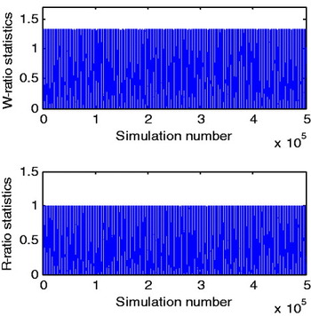
So, for a geometry defined by Qâ, the user controllable fail-rate has to be pre-defined within the range of the upper bound, (0·3260) and the lower bound (0), and any chosen fail-rate beyond the this range is meaningless. The implications for the normally used statistic tests, e.g., R-ratio, F-ratio, W-ratio, Difference test, Projector test, are that there should be upper bounds and lower bounds for the chosen critical values as well, as shown in Figure 6 within the IA estimation framework, for example, the upper bound for W-ratio in this geometry is 1·33. If a user choose a critical value larger than 1·33, the user can be advised that there won't be any integer outcomes, which coincides with the IA fail-rate as 0. Similarly, due to the special structures for R-ratio and F-ratio, their critical value bounds are always 0 and 1.
The simulated statistics for W-ratio and R-ratio tests with the geometry of Qâ.
If the strengthening of the geometry changes, for instance, with the increasing of k, the ILS success-rate for Qâ increases, whereas the fail-rate decreases. Before the ILS fail-rate comes close to 0, the IA fail-rate upper bound has to be narrowed down due to the decreasing of the ILS fail-rate, and then the choice of the pre-defined fail-rate has to be narrowed down as well. As shown in the left side of Figure 7, the allowable chosen area of the IA fail-rate is plotted in grey, and any IA fail-rate above the upper bound (solid blue line) is not appropriate for IA-based ambiguity validation. On the right side of Figure 7, the correspondingly upper bounds for W-ratio's critical values have been plotted. It can be seen there are indeed upper bounds of the critical values for different geometry. As long as the ILS success-rate is extremely close to 1, it implies that almost all the simulated float solutions are within the correct ILS pull-in region, and almost all the most likely integer candidates from LAMBDA are the correct ones with an extremely small fail-rate. An adjustment of the IA fail-rate only tunes the acceptance region, which balances the IA success-rate and the undecided-rate, and hardly changes the fail-rate. Consequently, the pre-defined fail-rate for the IA estimation can be extremely close to 0. In this case, the chosen critical value for W-ratio should be very close to 0, regardless of the upper bound. Ambiguity validation in such an extreme geometry becomes trivial.
Left: The ILS fail-rate of Qâ,k (solid blue line) and the allowable chosen of the IA fail-rate (grey area), right: W-ratio upper bounds for different k.

4.2 Practical Implications
The upper bound for the IA fail-rate is defined by the fail-rate from ILS. Unfortunately, it is very complex to evaluate the ILS fail-rate. Simulation with a large sample size is an ideal way, but the computation burden increases dramatically with the increasing of the ambiguity dimension. As alternatives, the user has to resort to the efficient approximation for the evaluation of the ILS fail-rate, for instance, the approximation based on the Ambiguity Dilution Of Precision (ADOP), as shown in Teunissen (Reference Teunissen1997), Verhagen (Reference Verhagen2005).
Two static data sets have been selected to analyse the upper bound and lower bound in real applications. Data set A is from two CORS stations (‘UNSW’ and ‘CHIP’) in Sydney, Australia, and data set B is from two NGS-CORS stations (‘CHAB and P235’) in California, America. Both of these data sets are processed epoch by epoch by a modified version of GNSS software RTKLIB, (Takasu and Yasuada, Reference Takasu and Yasuda2009), with single-frequency only and dual-frequency respectively. During the data processing, an elevation dependent stochastic model was applied. In each data set, several epochs were eliminated due to their inadequate quality, and there are 5747 epochs and 2879 epochs for data set A and B. A summary of the data sets can be found in Table 1.
Static data summary.
To perform an ambiguity validation procedure by the pre-defined IA fail-rate, the users should then choose the fail-rate they preferred. However, a meaningful chosen of the IA fail-rate should be based on the upper bound. As shown for data sets A and B in Figures 8 and 9, the blue lines are the ILS fail-rates, which were calculated with the knowledge of approximation of the ILS success-rate by the ADOP. Providing the ILS fail-rate as the upper bound, it can be shown that the upper bound varies with the epoch number, and for the user's benefits, the knowledge of the upper bound for the IA fail-rate allows the user to choose a reasonable fail-rate at the designing stage. For example, the dual-frequency upper bound (the upper figures) can help the user to choose different fail-rates to obtain relevant success-rates for different epochs, even before they conduct a GNSS survey. In addition, it should be noted that the smaller (or larger) the IA fail-rate upper bound, the stronger (or poorer) the ambiguity geometrical strength is, especially when the IA fail-rate upper bound is 0, the geometry is strong enough to theoretically guarantee the resolved ambiguities are correct. So, for the dual-frequency scenario, in epochs around 1000, 2500, 3500 for data set A and epochs around 1300, 2500 for data set B, the user is advised of enough confidence to choose the IA fail-rate close to the upper bound, so as to allow more correct acceptances.
Upper bounds and lower bounds for IA fail-rate in case of single-frequency and dual-frequency for data set A.

Upper bounds and lower bounds for IA fail-rate in case of single-frequency and dual-frequency for data set B.

For the single-frequency scenario, the user has been informed a large range for the chosen IA fail-rate. The larger of the IA fail-rate ranges indicates the poorer of the ambiguity geometrical strength. Therefore, a wise decision is to narrow down the acceptance region to exclude more incorrect acceptances.
In Figures 10 and 11, the upper bounds for the Wa-ratio statistics are plotted for both data sets. There are upper bounds for different scenarios. The dash red lines show the dual-frequency upper bounds for the Wa-ratio tests and the solid blue lines show the upper bounds for single-frequency. As a result, if the user is going to validate the resolved integer ambiguities by WIA, the chosen critical value in each epoch has to be smaller than that of the upper bound in the corresponding epoch. Otherwise, no integer outcomes can be obtained. The same holds true for the difference test and the projector test, for which the user should be reminded of the upper bound for the selection of critical values.
Upper bounds for Wa-ratio in case of single-frequency (solid blue) and dual-frequency (dash red) for data set A.

Upper bounds for Wa-ratio in case of single-frequency (solid blue) and dual-frequency (dash red) for data set B.

5. CONCLUSION
Ambiguity validation is an important step for precise GNSS positioning and the IA estimation has been established to provide a framework for the ambiguity validation methods. Consequently, using the pre-defined fail-rate to validate the resolved ambiguities is more user-specific than choosing the critical value. Due to the importance of the IA fail-rate, in this contribution, we have analysed the upper bound and the lower bound for the determination of the IA fail-rate. It has been shown that a chosen IA fail-rate should be within the upper bound and the lower bound, and since the IA fail-rate and the critical value are connected according to simulation, these bounds for the fail-rate also imply there are upper bound and lower bound for the critical values of the normally used ambiguity validation methods. Two dimensional simulations have been performed to illustrate the benefits of the upper bound and the lower bound for the IA fail-rate. In addition, in cases where the ILS fail-rate comes extremely close to 0, as an upper bound, the IA's fail-rate should be chosen also as extremely close to 0, and this indicates that under such a strong geometry, all the float solutions can be accepted with an extremely small fail-rate.
In terms of practical implications, the approximation based on the ADOP value for evaluating the ILS success-rate is suggested, and then the upper bound for the IA fail-rate can be determined. Therefore, the user can acquire the knowledge of the range for the purpose of choosing the reasonable fail-rate they preferred. Real GNSS data sets have been processed to reveal the procedure of determining the IA fail-rate in a reasonable range, and also the implicated upper bound for the critical values has been presented. It turns out that users should be aware of the useful upper bound and the lower bound on the basis of the IA estimation.
It is worth mentioning that neither the traditional ambiguity validation tests nor the IA based method considers the influence of the biased float solution. Future research will be focused on the formula derivation for the bounds of the critical values as well as analysing how large a bias can cause a wrong ambiguity validation decision.
ACKNOWLEDGEMENTS
The first author would like to acknowledge the Chinese Scholarship Council (CSC) for supporting his PhD studies at The University of New South Wales, Sydney, Australia. The authors also would like to thank the anonymous reviewers for their valuable comments and suggestions.


