


1. Introduction
Turbulent mixing plays a key role in regulating the thermohaline circulation of the ocean as originally described by the theoretical model of Munk (Reference Munk1966). A key result from Reference MunkMunk's (Reference Munk1966) analysis was the rather large value for the vertical diffusivity representative of the ocean (Naveira Garabato & Meredith Reference Naveira Garabato and Meredith2022), and this has inspired a considerable amount of theoretical, experimental and field research over the past half-century on the controls on the mixing of a stratified fluid (Osborn Reference Osborn1980; Ledwell et al. Reference Ledwell, Montgomery, Polzin, St. Laurent, Schmitt and Toole2000; Waterhouse et al. Reference Waterhouse2014; Ferrari et al. Reference Ferrari, Mashayek, McDougall, Nikurashin and Campin2016; McDougall & Ferrari Reference McDougall and Ferrari2017; Naveira Garabato et al. Reference Naveira Garabato2019; Spingys et al. Reference Spingys, Garabato, Legg, Polzin, Abrahamsen, Buckingham, Forryan and Frajka-Williams2021).
Field studies have shown that there is considerable spatial variation in the mixing, typically being weaker in the ocean interior and more intense near the ocean floor and boundaries (Polzin et al. Reference Polzin, Toole, Ledwell and Schmitt1997; Waterhouse et al. Reference Waterhouse2014). The process of mixing involves a combination of internal wave breaking and shear-driven mixing (Winters et al. Reference Winters, Lombard, Riley and D'Asaro1995; Caulfield Reference Caulfield2021; Howland, Taylor & Caulfield Reference Howland, Taylor and Caulfield2021; Mashayek, Caulfield & Alford Reference Mashayek, Caulfield and Alford2021), as well as localised boundary mixing (Thorpe Reference Thorpe2007; Echeverri et al. Reference Echeverri, Flynn, Winters and Peacock2009; Winters Reference Winters2015; Jagannathan, Winters & Armi Reference Jagannathan, Winters and Armi2017; Polzin & McDougall Reference Polzin and McDougall2022) which then interacts with the remainder of the fluid. From a theoretical perspective, turbulent mixing in a stratified fluid involves a number of complex processes, and depends in detail on the balance between the dissipation of kinetic energy, the generation of potential energy, the ambient stratification and both the mean velocity and the shear (Osborn Reference Osborn1980).
Armi (Reference Armi1978) suggested that transect data near the Bermuda Islands showed enhanced mixing near the boundaries and topographic features, as characterised by the step-like structure of the temperature and salinity field. It was suggested that this layering is advected laterally and gradually becomes smoothed into a more continuous profile away from the boundaries, leading to an effective vertical diffusivity averaged across the basin,  $\bar {\kappa }$, as given by the relation
 \begin{equation} \bar{\kappa} = \kappa_{bound} A_r , \end{equation}
where  $\kappa _{bound}$ is the vertical eddy diffusivity at the boundary and $A_r$ is the ratio of boundary-to-basin cross-sectional area. This equation assumes that the effect of boundary mixing is the primary contributor in determining the bulk diffusivity ( $10^{-4}\ \text {m}^2\ \text {s}^{-4}$), which is an order of magnitude greater than the local measurements of the interior diffusivity ( $10^{-5}\ \text {m}^2\ \text {s}^{-5}$).
A number of laboratory experiments have been reported in which an initial two layer stratification was mixed by a local mixer at the end of a long experimental tank. In many of these experiments, as the stratification evolves through vertical mixing in the boundary region, lateral intrusions of the mixed fluid spread from the boundary into the interior (Ivey & Corcos Reference Ivey and Corcos1982; Thorpe Reference Thorpe1982; Phillips, Shyu & Salmun Reference Phillips, Shyu and Salmun1986). As a result, surfaces of constant density tend to remain approximately horizontal, with the stratification evolving at the same rate in both the boundary and interior regions. Phillips et al. (Reference Phillips, Shyu and Salmun1986) showed that, even if the mixing occurs on a sloping boundary, a similar pattern of mixing arises, albeit with a secondary circulation which occurs due to the no-flux condition at the boundary (see also Garrett Reference Garrett1990; Woods Reference Woods1991). The presented work involves mixing in a vertical plane, and so our results do not depend on processes specifically associated with a sloping boundary.
Many of the experiments (Ivey & Corcos Reference Ivey and Corcos1982; Thorpe Reference Thorpe1982; Phillips et al. Reference Phillips, Shyu and Salmun1986) involved a transient flow, and focused on quantifying the intensity of the mixing in the boundary region by exploring the balance between the kinetic energy supplied through the mechanical agitation and the evolution of the potential energy associated with the stratification. There has been less focus on the mechanisms of buoyancy and tracer transport by such boundary mixing, especially in steady state, where there is a constant vertical flux of buoyancy. In systems where the evolution of buoyancy and tracer can be measured, it is of interest to understand how the bulk mixing is related to the spatial distribution of the mixing through the system, and we explore this in the present paper.
In particular, we investigate the evolution of the salinity and also of a passive tracer in both the interior and boundary regions of a stratified fluid that is mixed in a localised region adjacent to the vertical wall of a laboratory tank and in which a buoyancy flux is supplied at the base and extracted at the surface. This arrangement, in which the imposed buoyancy fluxes are imposed, represents a generalisation of the processes that drive the buoyancy fluxes in ocean systems, where vertical transport is driven by a combination of advection and mixing and maintained through the supply of cold, saline water at large depths, is one where surface heating provides a flux of heat at the ocean's surface and the detailed balance between evaporation and precipitation provides a supply of fresh water closer to the surface. Our simplified system provides a useful means to investigate the effects of local mixing in steady-state systems. In the oceans, the turbulent mixing is driven by a combination of tidal motions and internal wave breaking that leads to a turbulent diffusive flux that is nonlinearly dependent on the strength of the buoyancy gradient. In this study, a vertically uniform, oscillating rake is used to generate the turbulence. We examine the steady-state density stratification and compare this with a reference experiment in which the mixing occurs through the whole tank. We then explore how the stratification evolves in response to a change in the source buoyancy flux.
In the boundary mixing experiment, we find that, in steady state, the vertical transport of salinity occurs primarily in the boundary region and there is negligible mixing of fluid or vertical transport of salinity in the interior of the space. In contrast, with mixing throughout the tank, we find that tracer injected into the fluid does become mixed vertically throughout the tank, even if the density field is in steady state (cf. Whitehead & Wang Reference Whitehead and Wang2008). If the boundary conditions change and there is a transient adjustment of the stratification, then we find, with boundary mixing, that a net upwards or downwards flow develops in the boundary region. This drives an opposite flow in the interior. If the density gradient becomes nonlinear, this leads to a divergence of the diffusive flux in the boundary region and a net lateral flow between the boundary and the interior which may be interpreted as the previously documented intrusion-like structures. These processes together lead to an evolution of the density profile in the interior. We develop a quantitative model for the transient evolution of the density in terms of the intensity of the local mixing in the boundary region, and test this with our experimental data.
The paper is structured as follows. First, we describe the experimental apparatus in § 2. In § 3, we present the results of our steady-state experiments and in § 4 we use these data to test a model for steady boundary mixing. In § 5 we describe a series of experiments in which the stratification evolves in time owing to a change in the boundary conditions, and in § 6 we test our model for the transient boundary mixing. In Appendix C we compare the model with new experimental results in which a two-layer stratification is mixed near the boundary for comparison with the earlier experiments of Ivey & Corcos (Reference Ivey and Corcos1982) and Phillips et al. (Reference Phillips, Shyu and Salmun1986). In § 7 we draw some conclusions.
In a companion paper (Li and Woods Part 2), we explore the additional interaction of a net upwelling with the buoyancy transport described in this paper. This builds on the results in the present paper, but the upwelling leads to a more complex, nonlinear density gradient as in the original model of Munk (Reference Munk1966). Again, we compare the difference in the mixing and transport of buoyancy and also of tracer between the boundary mixing and interior mixing regimes.
2. Experimental apparatus
The experiment (figure 1) involves mechanical mixing of a salt-stratified fluid by an oscillating rake of vertical bars of diameter  $d = 1$ cm spaced $1$ cm apart. By controlling the horizontal amplitude of oscillation of the rake we can produce either local boundary mixing or mixing across the full lateral extent of the tank. The experimental tank is of length $L = 120$ cm, width $B = 10$ cm, height 60 cm and the fluid in the tank is maintained at a depth of $H = 55$ cm. To investigate boundary mixing (BM), the rake is driven by an in-house manufactured pneumatic system and oscillates back and forth a distance $a = 10.6$ cm at an approximately constant speed $U = ( 13.1 \pm 0.66 ) \text { cm s}^{-1}$ and impulsively changes direction once reaching the end of each stroke. The amplitude and speed of the oscillations can be set, but these values have been chosen to produce vigorous mixing and minimise sloshing in the tank. To investigate whole-tank (WT) mixing, the rake is driven by an electric motor and travels at the same speed $U = ( 13.1 \pm 0.3 )\text { cm s}^{-1}$ from one end of the tank to the other and then changes direction impulsively.

There are simple nozzles at the top and bottom of the tank through which fluid may be injected or extracted. Two nozzles are paired together to reduce the flow speed. The nozzles are positioned so that fluid is injected and extracted at approximately the same depth while aiming to minimise short circuiting of fluid. At the surface, the fresh water is injected through the nozzles which sit above the nozzles through which tank fluid is extracted. At the base of the tank, saline fluid is injected through nozzles which sit below the nozzles through which tank fluid is extracted. The nozzles are simple fittings, approximately 1 cm in diameter, and attached to the end of the tubing which points horizontally in the ‘width’ direction. Fluid is supplied and removed at the same rate to maintain a buoyancy flux at that depth, while driving no net flow through the system. The pumping of fluid disturbs the fluid only in the neighbourhood of the nozzles, and does not have a significant impact on the flow field as compared with that produced by the mechanical stirring. By measuring the flow rate and salinity of the supply and extract fluid, we are able to determine this net buoyancy flux at the base and surface of the tank. The fluid is pumped in or out using Watson Marlow peristaltic pumps.
Three configurations are described in this paper: (a) an experiment with buoyancy fluxes at both the base and top of the tank in which the system reaches steady state (§ 3); (b) an experiment with a surface buoyancy flux only in which an initial linear stratification evolves to a well-mixed state (§ 5); and (c) an experiment in which the tank initially has a two-layer stratification, analogous to earlier studies (Appendix C). For experiments with a net buoyancy flux at the base of the tank, we injected fluid of salinity  $S_B \sim 0.08$ g cm $^{-3}$ with volume flux $Q_B \sim ( 5.8 \pm 0.6)$ cm $^3$ s $^{-1}$ and extracted an equal volume flux of fluid from the base of the tank. In the case with a net buoyancy flux at the top of the tank, fresh water with salinity $S_T \sim 0$ is injected at the top-most nozzle at a rate of $Q_T \sim (5.0 \pm 0.6)$ cm $^3$ s $^{-1}$ and an equal volume of fluid is extracted from the top of the tank. The volume flux of injected fluid can drift and careful manual adjustments to the extracted fluid flow rate are made to keep the volume constant. The parameters used for the different experimental series are summarised in table 1.
Table 1. Parameters used in the presented steady-state and transient experiments. The mixing type can be (a) locally intensified, denoted as BM or (b) uniformly distributed, denoted as WT mixing. As described in the text, fresh fluid is injected at rate  $Q_T$ at the surface of the tank and fluid with salinity $S_B$ is injected at rate $Q_B$ at the bottom of the tank.

Salinity profiles were taken by sampling approximately  $5\ \text {ml}\unicode{x2013}10\ \text {ml}$ of fluid at vertical intervals of 5 cm using a long, thin pipe connected to a syringe. The salinity of the samples was measured using a digital refractometer in units degrees Brix to 1 decimal place and converted to units $\text {g cm}^{-3}$ using a conversion table (Haynes, Lide & Bruno Reference Haynes, Lide and Bruno2016). Salinity samples taken at the two ends of the tank at the same height coincided within measurement error, suggesting the surfaces of constant salinity were nearly horizontal. The data presented in the paper correspond to measurements from the right-hand side (turbulent side in the case of BM, see figure 1) of the tank for consistency across the experiments.
2.1. Release of dye into experiments
In some experiments presented in this paper, dye is introduced into the tank to visualise the flow. Two methods that were used to introduce dye into the tank are described herein.
For the primary method, which is used to produce horizontal lines of dyed fluid, fluid is slowly injected or extracted from nozzles on the left-hand side of the tank which point towards the interior of the tank (figure 1). The nozzles are simple fittings attached to the end of tubing, and are attached to the side of the tank at heights of 25 and 45 cm above the base of the tank. To produce the horizontal lines, the experiment is paused and the pumps and mechanical agitation are turned off. Fluid is extracted slowly through the nozzles using a syringe, which is then mixed with coloured food dye, and it is then reinjected slowly back in at the same depth. Before the dye is reinjected, its density is checked and if necessary adjusted so that it matches the original density. The fluid spreads slowly and laterally upon reinjection, and is left to do so for an hour, upon which the spreading has mostly stopped. At this point the experiment is resumed and the pumps and mechanical agitation are turned back on.
The other method, used only once in § 3.2, involves the release of a cloud of dye into the turbulent region. Dye is mixed with fluid of salinity  $S_B$ and squirted downwards into the turbulent boundary region near the base of the tank using a syringe attached to a long, thin needle. This injection of fluid produces a small turbulent jet that dissipates quickly in the turbulence of the mechanical agitation.
3. Steady-state observations
In this section, we present a series of experiments in which we supply a constant buoyancy flux to the base and remove a buoyancy flux from the surface of the experimental tank. In this configuration, the system reaches a steady state with a continuous transport of buoyancy through the depth of the tank and we investigate two configurations in which the mechanical mixing is either local to one end of the tank (BM) or uniformly distributed (WT mixing).
First, we present experimental data showing the convergence of the system to steady state. Secondly, we inject dyed fluid to illustrate the flow patterns by assessing the time evolution of parcels of dyed fluid.
3.1. Steady state
The final stratification generally does not depend on the starting stratification. The system is deemed to have reached a steady state once the salinity profiles are steady and the flux of salinity supplied to the base of the tank matches the flux of salinity removed from the top of the tank. We then check that these salinities do not vary beyond measurement error over an interval of approximately  $2$ hours. An example illustrating the convergence to steady state for the data in experiment 1 (BM) is shown in figure 2. Here, we plot the salinity profiles as a function of time. After approximately five hours it can be seen that the salinity profiles converge to a nearly linear vertical profile. The convergence to steady state is then quantified by calculating the root-mean-square (r.m.s.) error between each profile $S_n(z)$ taken at time $t_n$ and the mean of a selection of converged profiles $\bar {S}(z) = \varSigma _{n=N}^M ({S_n(z)}/({M-N})$:
 \begin{equation} {RMSE}_n = \frac{ \sqrt{\displaystyle \frac{1}{H}\int_0^H[ \bar{S}(z)-S_n(z) ]^2\,{\rm d}{z}}}{\displaystyle \frac{1}{H} \int_0^H\bar{S}(z)\,{\rm d}{z}}.\end{equation}
After six hours, the error decreases to a value of approximately  $5\,\%$ and remains smaller than this value for the duration of the experiment. This pattern is generally true for all steady-state experiments.

Figure 2. Experimental data (experiment 1) taken showing convergence of system to steady state. (a) Vertical salinity profiles as the stratification develops. The profiles are chronologically coloured blue–red–purple, and within each coloured subset also differentiated in order by: crosses and open circles; solid and dashed lines. A steady profile taken as an average of the profiles once the experiment has converged to steady state is plotted as a thicker black line. The salinities of the top and bottom fluid inputs are marked with red and blue arrows, respectively, for reference. (b) Salinity of the extracted fluid (solid) and the injected fluid (dashed) for the top (red) and bottom (blue) sets of nozzles as a function of time. (c) The r.m.s. error (as described in the text) between the profiles and the mean of steady profiles as a function of time.
We also plot (figure 2a) the net supply of salinity to the base of the tank (blue dashed and blue solid lines) and the net removal of salinity from the top of the tank (red dashed and red solid lines) as a function of time. These data also appear to converge to a steady state after six hours. The difference between the top and bottom buoyancy fluxes is smaller than  $4\,\%$ of the mean value.
3.2. Boundary mixing flow description
Experiment 2 (BM) converges to steady state after approximately 9.5 hours. At this time, two lines of red dye are injected into the tank interior at heights of 25 and 45 cm. The reinjected cloud of dye spreads slowly and laterally at this depth and then, after approximately one hour, the experiment is resumed, which we label as time  $t = 0$ mins in figure 3, or time $t=9.5$ hours in figure 2. The dye study runs for a period of approximately three hours from the time of injection, which is contained fully within the data shown in figure 2.

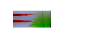
Figure 3. Illustration of flow patterns in the BM, steady-state experiment (experiment 2). (a) Snapshots of the front view, see figure 1 of the evolution in time of two lines of dye along with two later injections of green dye. Two lines of red dye are initially injected into the tank interior away from the mixing grid and laterally spread with no vertical mixing, with images detailing their state at times  $t =$ (ai) 0 mins, (aii) 40 mins, (aiii) 80 mins after the injection of red dye. After 120 minutes, green dye is released at the bottom of the mixing zone at the right-hand side of the tank and turbulently mixes (av–aviii). (aiv) Schematic summary of the flow. Fluid in the interior of the tank remains quiescent, and does not mix or move. Fluid in the turbulent mixing region mixes in eddy structures, which in turn drives oscillatory movement in the fluid that is near the edge of the turbulent region, which can be seen to oscillate towards and away from the turbulent mixing region. (b) False-colour time series of the red dye intensity of a vertical line in the interior, approximately 40 cm from the left wall of the tank, containing the red dye lines (after subtracting background and cropping the intruding green dye). (c) True-colour time series of a horizontal line (chosen at middepth), starting from when the stronger injection of green dye, into the BM region, reaches midway up the tank ( $t = 130$ mins). Note that the movement of the rake can be seen in this time series as an oscillating black structure.
In figure 3 we present a series of photographs showing the evolution of the dye. For two hours the lines of dye in the interior fluid spread laterally towards the mixing region, and tiny amounts of dye are mixed in the turbulent region but this cannot be seen in the photographs. The bulk of the red lines of dye show no net vertical movement and very little mixing (figures 3ai–3aiii); this can be seen in a time series of the dye concentration of a vertical line in figure 3(b). Afterwards. green dye is squirted into the bottom of the turbulent mixing region using a long, thin needle attached to a syringe in two phases: at first, a weak pulse of green dye is released (for image analysis in figure 6) and four minutes later a stronger pulse of green dye is released (for clarity in the true-colour photographs that can be seen in figure 3(av–avii). We observe that the green dye mixes rapidly and is confined to the width of the turbulent mixing region and, within sixteen minutes, also mixes vertically through the depth of the tank. Throughout this process, there is negligible lateral transport. This can be inferred from the stationary lines of red dye, which both do not move vertically or mix. Over a longer time scale, there is an additional, slow exchange of fluid between the boundary and the interior, and this can be seen over the next fifty minutes, where a time series of a horizontal line of pixels (figure 3c), taken at mid depth, shows the width of the green zone growing very slowly over time. The edge of the green dyed fluid has a series of intrusion-like structures that oscillate towards and away from the BM region.
The flow appears to be partitioned into three regions. Near the oscillating mixing rake, on the right-hand side of the tank, there is a turbulent region with width of approximately 25–40 cm, marked by the horizontal extent of the red lines. On the left-hand side of the tank, far from the mechanical mixing, is a largely quiescent region where there is no mixing or net flow, but where there appears to be small oscillatory vertical movement from surface gravity waves. Between the quiescent interior and the turbulent mixing zone is an intermediate region in which there is a series of intrusions which move into and out of the BM zone but there remains a distinct interface between the green and clear fluid. In figure 3(aiv) we summarise this picture schematically. The vertical transport of salinity appears to be dominated by the turbulent diffusive mixing in the turbulent boundary region, with negligible transport in the interior region.
3.3. Whole-tank mixing flow description
We now illustrate the flow patterns in the case of WT mixing. In this case the mixing rake traverses the length of the tank with a speed approximately similar to that in the case of BM.
A single line of dye is introduced in a similar fashion to that described in § 2.1. Five photographs (figure 4ai–av) illustrate the evolution of this line of dye, which mixes vertically and laterally as the rake continuously stirs the fluid.

Figure 4. Images detailing the evolution of a dye line in steady state in the case of WT mixing (experiment 3). (ai–av) Photographs showing the spreading of a dye line with WT mixing for thirteen minutes after introduction. (b) False-colour time series of the dye concentration of a vertical line in the case of WT mixing. (avi) Schematic summary of the flow. Circular arrows represent the eddies that are left in the wake of the rake's traversal. The dissipation of these eddies leads to mixing of the fluid, which can be visualised by the spreading of the red dye, represented with jagged arrows.
The rake traverses the entirety of the tank approximately every half-minute. The rake traverses at a constant speed through the cloud of dye, which is in turn mixed by the dissipation of eddies that are left in the trailing wake. The eddies appear to be uniform in intensity across the horizontal extent of the tank, and we observe that the dye mixes at approximately the same rate across the tank subject to these eddies. A time series of a vertical line of pixels shows the vertical spread of the dye as a function of time (figure 4b). Dye reaches the bottom of the tank after approximately two minutes and the top of the tank after six minutes. A schematic summarising the flow patterns is shown in figure 4(avi).
4. Steady-state model
In § 3 we showed that, in the case of WT mixing, mixing occurs approximately uniformly throughout the tank, as the dye, although not uniformly mixed horizontally, has a vertical extent that increases at approximately the same rate throughout. In the case of BM, dye and salinity vigorously mix in the region with mechanical mixing but are quiescent elsewhere. In this section, we present a simple one-dimensional diffusion model to compare the effective diffusivity associated with the buoyancy transport and that associated with the dye mixing.
4.1. Calculating the bulk diffusivity for BM
In both cases of boundary and WT mixing, mixing by the mechanical turbulence transports salt through the depth of the tank. If we describe this with a tank-averaged effective diffusion process then the effective diffusivity can be calculated based on the steady-state linear salinity stratification and the buoyancy fluxes supplied at the upper and lower boundaries.
The salt fluxes on the top and bottom boundaries are given by  $Q_TS_t, \ Q_B ( S_{B} - S_b )$, respectively, where $S_t, \ S_b$ are the salinities of output fluid from the top and bottom boundaries of the tank, respectively. As noted previously, the difference between these salt fluxes is less than 4 % once the experiment reaches steady state. The effective diffusive mixing, $\bar {\kappa }$, drives a salinity flux over the cross-sectional area of the tank, $BL$, with flux $-\bar {\kappa } BL ({{\rm \Delta} S}/{{\rm \Delta} z})$ where ${{\rm \Delta} S}/{{\rm \Delta} z}$ is the salinity gradient.
The effective area-averaged diffusivity  $\bar {\kappa }$ may be calculated by averaging the boundary salinity flux at the top and bottom of the domain as given by
 \begin{equation} \frac{1}{2}[ Q_T ( S_t ) + Q_B ( S_{B} - S_b ) ] ={-}\bar{\kappa} BL \frac{{\rm \Delta} S}{{\rm \Delta} z}.\end{equation}
 For each value of  $\bar {\kappa }$, the salinity gradient ${{\rm \Delta} S}/{{\rm \Delta} z}$ is calculated. We then fit the linear profile $S(z)$ through the steady-state salinity profiles, minimising the error between the fitted profile and the experimental data as given by the r.m.s. error between the data and the matched salinity profile $\mathcal {S}(z)$:
 \begin{equation} {RMSE} = \frac{1}{N} \sum_n^N \frac{ \sqrt{\displaystyle \frac{1}{H}\int_0^H[ \mathcal{S}(z)-S_n(z) ]^2 \,{\rm d}{z}}}{\displaystyle \frac{1}{H}\int_0^H\mathcal{S}(z)\,{\rm d}{z}}.\end{equation}
 Over the range of  $\bar {\kappa }$, a range of possible salinity profiles $S(z)$ can match the data within the experimental error. An example of the resulting fit is shown in figure 5(a) (experiment 1).

Figure 5. (a) Example of fitting linear solution to the experimental data in experiment 1 (steady state), resulting in  $\bar {\kappa } = 0.12 \text { cm}^2\ \text {s}^{-1}$. (b) The r.m.s. error as a function of the calculated value for $\bar {\kappa }$ using (4.1). The salinity of the basal input fluid takes the values $S_B = 0.04 \text { g cm}^{-3}$ (experiment 4), $0.082 \text { g cm}^{-3}$ (experiments 1, 2), $0.12 \text { g cm}^{-3}$ (experiment 5).
For experiments 1, 2, 4 and 5 given in table 1, this r.m.s. error is less than 10 % for values of  $\bar {\kappa }_{BM}$ in the range
 \begin{equation} \bar{\kappa}_{BM} = (0.13 \pm 0.03)\text{ cm}^2\ \text{s}^{{-}1}.\end{equation}
We note that there is a small difference in the salinity at the top and base of the tank relative to the linear gradient model associated with vertical turbulent transport with effective eddy diffusivity  $\kappa$. Near the base and top of the tank, there is some additional turbulent mixing owing to the injection and extraction of fluid that drives the net buoyancy flux. However, for simplicity, in developing the model, we assume the diffusivity is constant across the tank.
In the case of WT mixing (experiment 3), a similar process is carried out to estimate the diffusivity. Again, we measure the vertical distribution of salinity and balance the interior diffusive flux with the salinity fluxes supplied at the boundaries. This gives that the bulk diffusivity for the WT mixing set-up is
 \begin{equation} \bar{\kappa}_{WT} = ( 0.29 \pm 0.06 )\text{ cm}^2\ \text{s}^{{-}1}.\end{equation}
4.1.1. Sensitivity to the imposed flow rate and rate of mixing
The flux of buoyancy across the stratification driven by the turbulent mixing from the oscillating rake is matched by the flux of buoyancy at the top and bottom of the tank associated with the injection and extraction of fluid at both locations. This flux depends on the salinity of injected and extracted fluid, which is indirectly set by the rate of mixing and by the imposed flow rate. Our experiments show that the vertical buoyancy flux through the tank depends on the flow rate through the supply and extraction nozzles, the salinity of the supply fluid and the rate of mixing of the rake, which have been varied within the ranges as described in § 2 and table 1. A similar experimental set-up, in which there was an imposed injection and extraction of fluid at the top and bottom of the tank, although with a different turbulent mixing mechanism, was reported by Petrolo & Woods (Reference Petrolo and Woods2019). The referenced study, using a similar mechanism to control the vertical buoyancy flux through the tank, provides additional details concerning the robustness of buoyancy transport as the flow rate changes. In particular, for that study, there is a case in which the vertical transport of buoyancy is limited by the rate of turbulent mixing.
4.2. Dye mixing in the WT mixing experiments
We now investigate the mixing of dye released into the interior of the tank, comparing its mixing with a simple diffusion model using the values estimated for the diffusivity from the buoyancy transport (§ 4.1).
We assume that the light intensity anomaly is linearly correlated with dye concentration within the values used (Cenedese & Dalziel Reference Cenedese and Dalziel1998). We choose a vertical strip within the tank and find the vertical distribution of dye as a function of time. We assume that the dye concentration,  $C$, evolves according to the diffusion equation with diffusivity $\bar {\kappa }$:
 \begin{equation} {\frac{\partial{C}}{\partial{t}}} = \bar{\kappa}\left( {\frac{\partial^2{2}}{\partial{C}^2}}{x} + {\frac{\partial^2{2}}{\partial{C}^2}}{z} \right) . \end{equation}
In the case of a non-uniform horizontal line of dye, this leads to the prediction that the concentration has the form
 \begin{equation} C(x, z, t) = F(x,t)\exp \left(-\frac{(z-z_0)^2}{4\bar{\kappa}(t-t_0) }\right),\end{equation}
provided the dye has not spread to the top and bottom boundaries of the tank. Here,  $F(x,t)$ is an amplitude term that is a function of the initial distribution of dye, which is approximately uniform over the measured section. Additionally, the dye appears to mix rapidly horizontally and as an approximation we focus on the vertical distribution of the dye.
The vertical distribution of the dye within the tank at each time can be fitted with a Gaussian profile to measure the thickness of the line of dye for comparison with the model. According to the model, the variance,  $\sigma ^2$, should increase linearly in time,
 \begin{equation} \sigma^2 = 2 \bar{\kappa} (t - t_0) .\end{equation}
Examples of the fits of the Gaussian profiles to the experimental data are shown in Appendix A in figure 11.
We look at mixing of the red line of dye released into the interior of the tank in the WT mixing (experiment 3). The measured variances (solid lines) are shown in figure 6(a) (blue) as a function of time along with the theoretical variance (dashed lines) (4.7), where  $\bar {\kappa } = \bar {\kappa }_{WT}(1 \pm 0.1)$ is the tank-averaged diffusivity calculated from salinity transport (4.4) with error margins shown by the dotted lines. The estimate of the diffusion coefficient associated with the mixing of the dye is consistent with the diffusivity estimated for the salinity transport for the first 500 seconds of the experiment.

Figure 6. (a) Variance of a Gaussian fit to the spreading of dye lines (solid) in the case of BM (red, experiment 2) and WT mixing (blue, experiment 3), compared with the theoretical spreading (dashed) with corresponding effective diffusivity  $\bar {\kappa }$ and $\pm 0.03 \ \text {cm}^2\ \text {s}^{-1}$ error margins (dotted). (b) Variance of a Gaussian fit to the spreading of green dye in the BM region (solid, experiment 2), compared with the theoretical spreading (dashed) with the intensified effective diffusivity, or boundary diffusivity, $\kappa _B$ and $\pm 0.08\ \text {cm}^2\ \text {s}^{-1}$ error margins (dotted).
4.3. Dye mixing in the BM experiments
First we look at the vertical mixing of red dye released into the interior of the tank (experiment 2). The variance of the vertical distribution of dye is shown in figure 6 by a solid line. This appears to be constant in time. This is compared with the theoretical variance (4.7) (dashed line), where  $\bar {\kappa } = \bar {\kappa }_{BM}$ is the tank-averaged diffusivity calculated from salinity transport (4.3). By comparison, we see that the dye shows no signs of mixing on this time scale.
Secondly, we look at the vertical mixing of the green dye in the turbulent boundary region in the case of BM (experiment 2). The intensified diffusivity in the boundary region, given by (1.1),  $\kappa _B = \bar {\kappa }({L}/{L_B})$, where $L = 120\text { cm}$, depends on the width of the turbulent BM zone which we estimate to be $L_B= (30 \pm 5) \text { cm}$ from figure 3(c). The variance of the vertical distribution of the green dye injected in the BM region (as shown in figure 3) is plotted (solid line) in figure 6(b) as a function of time, along with the theoretical variance (4.7) (dashed and dotted lines), using the value $\kappa _B = (0.56 \pm 0.08)\ \textrm{cm}^2\ \textrm{s}^{-1}$ as measured from the salinity field. The agreement is good suggesting that the local dye and salt mixing processes are equivalent.
5. Transient experiment observations
The previous experiments have shown that, in steady state and with BM, the interior fluid is quiescent and does not mix or have any net movement. The BM experiments (experiments 6 and 7) in this section investigate the case in which the stratification changes in time to determine how the interior fluid density evolves when there is no interior turbulent mixing. We start with an initial stratification, that is either linearly stratified (experiment 6) or well mixed (experiment 7), which then evolves in time when the buoyancy flux at the base of the tank is removed, and where we inject fresh fluid at the surface while also removing an equal volume of fluid from the tank.
In experiment 7 we add a line of red dye and a line of green dye at heights of  $25 \text { cm}$ and $45 \text { cm}$ and track how they move in time. These are added in a fashion similar to the experiments described in § 2.1.
In figure 7 we present photographs showing the evolution of the dye as the experiment progresses. The two lines of green and red dye do not undergo any turbulent mixing whilst in the interior. The lower line of green dye downwells at a faster speed than the higher line of red dye and, after forty minutes, most of the green dye has reached the base whilst red dye moves only a few centimetres. Near the bottom boundary there appears to be a boundary zone a few centimetres deep due to the no-flux condition applying at the base of the interior portion of the tank. This region features strong horizontal advection and we observe that the green dye travels quickly across the length of the tank towards the mixing rake over the course of approximately five minutes. Upon reaching the mixing rake, the green dye can be seen to mix upwards from the base, whilst some fluid intrudes back into the interior of the tank. From  $t = 80$ minutes to $t = 200$ minutes the green dye mixes in the boundary region whilst a front of green fluid detrains from the mixing zone into the interior. In contrast, during this time the red dye maintains a distinct boundary with the surrounding clear fluid as it downwells towards the bottom-left corner of the tank. The divergence of this downwelling flow with depth leads to a change in shape of the red dye pulse, which becomes thicker in the vertical and of smaller horizontal extent.

Figure 7. Overview of the time evolution of two lines of green and red dye in experiment 7 from time of injection. (a) Photographs of the dye evolution as the experiment progresses (see figure 1 for camera location). The snapshots (aiv–avi) in the right-hand column have symbols overlain which correspond to the theoretical evolution predicted by the model in § 6, starting from the initial positions at  $t = 80\text { mins}$. The differing symbols (dot, star, triangle) differentiate the particles which are in turn entrained (where triangles disappear at $t = 140 \text { mins}$ and stars disappear at $t = 200 \text { mins}$). (b) Schematic overview of the flow pattern. The shape of the green front is motivated by the photographs. Left-pointing arrows representing the depth-varying lateral velocity are schematic representations of the model velocity predictions in § 6. (c) Vertical salinity profiles, ordered chronologically (blue–red, and, within each coloured subset, crosses–open circles; solid and dashed lines).
There is a continuous removal of salinity from the surface of the tank and the salinity stratification eventually adjusts to a self-similar shape, with decreasing salinity as the experiment progresses. Salinity profiles taken from this experiments are shown in figure 7(c).
6. Transient model
In this section we present an analytical model for the transient evolution of the system as described in § 5, using equations for a local and global mass flux balance. The model predictions are then compared with the experimental data on the evolution of the salinity profile and also the distribution of the profile of dye.
6.1. Analytical model
Previous studies (Hopfinger & Toly Reference Hopfinger and Toly1976; Ivey & Corcos Reference Ivey and Corcos1982; Thorpe Reference Thorpe1982; Phillips et al. Reference Phillips, Shyu and Salmun1986) have proposed models for the mixing length scale  $L_B$ and turbulent diffusivity $\kappa _B$ in terms of the experimental parameters. The dynamics within the turbulent mixing region can be described by the time-averaged equations for the local mass conservation and by the vorticity equation (see Woods Reference Woods1991).
In the transient experiments, we envisage that the removal of the buoyancy flux supplied to the base of the tank results in an eventual decrease in the buoyancy of fluid parcels in the lower part of the BM region subject to the continued mixing from above. This leads to an upwards, buoyancy-driven flow in the boundary region, and an equal and opposite flow in the interior as seen by the downward migration of the lines of dye in the interior of the fluid. Intrusions form as a result of any divergence of the flow in the boundary region, which then change the spacing between interior isopycnals in a manner consistent with the changing system stratification, even though there is no evidence of mixing of the interior fluid parcels themselves. The flow in each region is exactly such that both regions appear to mix with an effective diffusivity, which is the same as the mean diffusivity,  ${\kappa _B L_B}/({L_I + L_B})$.
We continue by assuming that the salinity is horizontally uniform with the exception being in the boundary layers which form at the top and bottom boundaries. We partition the tank into two regions; the BM zone with a uniform turbulent diffusivity and the quiescent interior as shown in figure 8. In the experiments, the horizontal lines of dye are injected and continue to remain horizontal as the stratification evolves, and so we assume that the vertical velocity is a function of depth only. Furthermore, in the steady-state experiments, the vertical buoyancy gradient is uniform and so we make the simplification that the turbulent diffusivity is independent of height. The convergence of flow in the boundary drives an intrusion into the interior, and by conservation of flux requires that the net vertical volume flux in the boundary region and interior is zero:
 \begin{equation} {\frac{\partial}{\partial{z}}} ( W_BL_B ) ={-}U ={-} {\frac{\partial}{\partial{z}}} ( W_IL_I ),\end{equation}
where  $U$ is the lateral flow into the interior from the boundary boundary, $W_I$, $W_B$ are the vertical velocities in the interior and boundary regions and $L_I$, $L_B$ are the widths of these two flow domains and subscript $I$ refers to the interior and subscript $B$ refers to the boundary. Similar to the approach taken by Munk & Wunsch (Reference Munk and Wunsch1998), integrating over a fluid control volume in the boundary region with diffusivity $\kappa _B$ gives that
 \begin{equation} {\frac{\partial}{\partial{t}}}(L_B S ) + {\frac{\partial}{\partial{z}}}( W_B L_B S ) - {\frac{\partial}{\partial{z}}} \left( L_B \kappa_B {\frac{\partial{S}}{\partial{z}}} \right) ={-}US, \quad L_I \leq x \leq L_I + L_B. \end{equation}
Combining this with (6.1) leads to the result
 \begin{equation} {\frac{\partial{S}}{\partial{t}}} + W_B(z,t){\frac{\partial{S}}{\partial{z}}} = \kappa_B {\frac{\partial^2{2}}{\partial{S}^2}}{z}, \quad L_I \leq x \leq L_I + L_B,\end{equation}
and similarly in the interior with molecular diffusivity,  $\kappa _I \ll \kappa _B$, we have
 \begin{equation} {\frac{\partial{S}}{\partial{t}}} + W_I(z,t){\frac{\partial{S}}{\partial{z}}} = \kappa_I {\frac{\partial^2{2}}{\partial{S}^2}}{z}, \quad x \leq L_I.\end{equation}
The fluid parcels in the boundary region undergo diffusive mixing whilst in the ambient there is negligible molecular diffusion. Note that there may be transport of fluid between the interior and boundary regions according to (6.1), and that the vertical velocities may vary with height and may be divergent as a result.

Figure 8. Overview of the idealised one-dimensional model describing the BM experiments where the domain is partitioned into a diffusive region with a stagnant ambient. Equations are derived by assuming that salinity is always horizontally uniform and balancing diffusive and advective fluxes across a fluid slice.
By considering a fluid slice across the whole domain, there is no net advective flux (by (6.1)) and so by adding (6.2) multiplied by the length,  $L_B$, and the complement of (6.2) multiplied by $L_I$ for the interior, we find that the divergence of the diffusive salinity flux suggests that the global stratification evolves according to the relation
 \begin{equation} {\frac{\partial{S}}{\partial{t}}} = \frac{\kappa_B L_B + \kappa_I L_I}{L_I + L_B} {\frac{\partial^2{2}}{\partial{S}^2}}{z} \approx \frac{\kappa_B L_B}{L_I + L_B} {\frac{\partial^2{2}}{\partial{S}^2}}{z}.\end{equation}
This equation suggests that the salinity evolves as if the diffusivities are averaged over the length of the tank. In the situation that the BM dominates,  $\kappa _B L_B \gg \kappa _I L_I$, as in the present paper, where $\kappa _I$ corresponds to the molecular mixing value, and so we can neglect the mixing in the interior. The assumption that the isopycnals remain horizontal relies on the time scale of the stratification, ${1}/{N}$ to be smaller than the time scale for turbulent mixing across the depth of basin in the boundary-mixed zone, ${H^2}/{\kappa _B}$, and this applies in the present experiments until the system becomes virtually uniformly mixed through the depth of the experimental tank.
In general, (6.3) may be rearranged so that the boundary velocity  $W_B$ may be expressed as
 \begin{equation} W_B = \frac{\displaystyle \kappa_B {\frac{\partial^2{2}}{\partial{S}^2}}{z} - {\frac{\partial{S}}{\partial{t}}} }{\displaystyle {\frac{\partial{S}}{\partial{z}}} } . \end{equation}
In the case that the system is in steady state,  ${\partial S}/{\partial t} = 0$ and, by (6.5), we also have that ${\partial ^2 S}/{\partial z^2} = 0$ and thus we have no vertical velocity in the boundary and also none in the interior, as was previously shown in the steady-state experiments. This model suggests that it is only possible to have vertical velocities if the buoyancy stratification is transitioning over time.
6.2. Boundary conditions
To describe the transient experiments (experiments 6 and 7), we impose the boundary condition that there is no buoyancy flux at the bottom boundary:
 \begin{equation} {\frac{\partial{S}}{\partial{z}}}(0, t) = 0.\end{equation}
At the top boundary the interior diffusive flux balances the flux for a matched inflow at a volume flux  $Q$ of salinity $S_{T} = 0$ and outflow of salinity $S(H, t)$:
 \begin{equation} -\kappa_B B L_B{\frac{\partial{S}}{\partial{z}}}(H,t) = QS(H, t), \end{equation}
where  $B$ is the width of the tank.
We look for a separable solution to find
 \begin{equation} S(z,t) = \sum_n A_n\exp(-\gamma_n t)\cos(\lambda_n z), \quad \lambda_n > 0,\end{equation}
where
 \begin{equation} \lambda_n(\kappa_B L_B)^2 = \frac{\gamma_n ( L_I + L_B )}{\kappa_B L_B} ,\end{equation}
and, in this case,  $\lambda _n(\kappa _B L_B) H$ satisfies
 \begin{equation} \tan \lambda_n H = \frac{Q H}{\kappa_B B L_B} \frac{1}{\lambda_n H}.\end{equation}
 With an initial stratification  $S(z,0) = S_0(z)$, the coefficients $A_n$ may be calculated using Sturm–Liouville theory to get that
 \begin{equation} A_n = \frac{\displaystyle \int_0^HS_0(z)\cos(\lambda_n z)\,{\rm d}{z}}{\displaystyle \int_0^H\cos^2(\lambda_n z) \,{\rm d}{z}}. \end{equation}
At long times the leading-order solution may be approximated by only the slowest decaying mode  $n=0$. Using (6.4) we can then express the interior velocity as
 \begin{equation} W_I = \frac{\gamma_0}{\lambda_0} \cot(\lambda_0 z),\end{equation}
excluding the bottom boundary layer. From (6.13) it follows that the streamfunction  $\psi$ satisfying $\boldsymbol {u} = \boldsymbol {\nabla } \times \psi \hat {\boldsymbol {y}}$ is
 \begin{equation} \psi = \frac{\gamma_0}{\lambda_0} \cot(\lambda_0 z)x,\end{equation}
and the height of a fluid parcel  $z(t)$ is given by
 \begin{equation} t - t_0 = \frac{1}{\gamma_0} \log \left(\frac{\cos(\lambda_0 z)}{\cos(\lambda_0 z_0)}\right),\end{equation}
where the height  $z=z_0$ at time $t = t_0$.
6.3. Comparison of the leading-order mode and the observations
The next mode has  $\lambda _1 \approx \lambda _0 + {{\rm \pi} }/{H}$ and so $\gamma _1 - \gamma _0 = ({\kappa _B L_B}/({L_B + L_I})) ({{\rm \pi} ^2}/{H^2} + 2({{\rm \pi} }/{H}) \lambda _0 ) \approx 5 \times 10^{-4}\ \text {s}^{-1}$. Our samples are generally taken at times $t_m \gg 10^{3}\ \text {s}$ and so the leading-order mode becomes a good approximation.
We can check the accuracy of the model presented in § 6 by calculating the r.m.s. difference between the leading-order model solution  $S^0(z,0) = A_0\exp (-\gamma _0 t)\cos (\lambda _0 t)$ and the $M-1$ experimental samples, $S_m(z)$ taken at time $t_m$, by
 \begin{equation} {Error} = \frac{1}{M-1}\sum_{m=2}^M \frac{\sqrt{\displaystyle \frac{1}{H}\int_0^H[ S^0(z,0)-S_m(z)\exp(\gamma_0 t_m) ]^2\, {\rm d}{z}}}{\displaystyle \frac{1}{H}\int_0^HS^0(z, 0)\,{\rm d}{z}}. \end{equation}
 The first ( $m=1$) data sample is used to find the initial condition for $S^0(z,t)$. We find that, at subsequent times, the difference between the model solution and the experimental data is less than 9 % for $\kappa _B$ within the range $\kappa _B L_B = 11.2\pm 0.8 \ \text {cm}^3\ \text {s}^{-1}$. This is consistent, although more constrained, than the value calculated in § 4. In figure 9, we scale the salinity profiles onto time $t=0$, $S_m(z)\exp (\gamma _0 t_m)$, and compare them with the leading-order model solution, $S^0$.

Figure 9. Salinity profiles from (a) experiment 7 and (b) experiment 6, scaled onto time  $t = 0$, $S_m(z)\exp (\gamma _0 t_m)$, using $\kappa _B L_B = 11.2 \text { cm}^3\ \text {s}^{-1}$. Overlain is the leading-order model solution from § 6, where the leading coefficient $A_0$ is calculated from the first ( $m = 1$) profile at time $t = 0$.
The best fit value for  $\kappa _B L_B$ is consistent with the value found in § 4. The salinity profiles from this model are consistent with the experimental profiles and are displayed in Appendix B in figure 12. This is further discussed in Appendix B.
6.4. Velocity profiles
We now compare the horizontal and vertical evolution of dye streaks in the experiment with the predictions of the model. Using the interior streamfunction given by (6.14) we predict the vertical and horizontal locations of interior dye parcels in experiment 7 with  $\kappa _B L_B = 11.2 \text { cm}^3\ \text {s}^{-1}$.
As shown in figure 7, green dye downwells in the interior, horizontally advects towards the mixing zone and intrudes back into the interior after vertically mixing. In figure 7(aiv), a series of points are marked which track the dye front at  $t = 80 \text { mins}$. These can be integrated in time using the streamfunction (6.14) and the subsequent points at times $t = 140 \text { mins}$ and $t = 200 \text { mins}$ are given in figures 7(av) and 7(avi).
We can plot a time series of a vertical line in the tank to track the vertical positions of the green and red dye lines in experiment 7. In figure 10(a) this is plotted and overlain with the vertical positions of the top and bottom edges of the dye line given by (6.15). Furthermore, in figure 10(b), we plot the horizontal position of the tip of the red dye line and this is compared with the model solution. There is reasonably good correspondence of the model prediction with the experimental observations providing support for the theoretical picture proposed herein.

Figure 10. (a) Time series of a vertical line in experiment 7 showing the time evolution of the vertical positions of the red and green lines. Overlain is the vertical tracking of the top and bottom edges of the dye lines using (6.15). (b) Time evolution of the horizontal distance of the tip of the red dye line plotted against model prediction (which follows the streamline described by  $\psi = \exp (-2.8) \text { cm}^2\ \text {s}^{-1}$).
7. Discussion
In this paper we investigated the steady-state mixing that occurs in a stratified fluid across which there is a constant flux of buoyancy. Through a series of laboratory experiments, we explored the spatial distribution of buoyancy transport when mixing occurs either uniformly across the tank or is confined to a region of the tank of narrow horizontal extent. As stated previously, the results presented in this paper are a result of mixing in a vertical plane, and in isolation of any sloped-induced effects. With BM, the transport of buoyancy occurred primarily through the turbulent boundary region while fluid in the interior did not mix or have any net movement. Between these two regions was a slowly growing region of intrusion structures with smaller transport over a much longer time scale. The same stratification developed throughout the tank. In the case of WT mixing, the salinity is transported uniformly through the tank in the vertical.
We also investigated the transient evolution of the stratification in the case of boundary mixing. Our experiments involved a removal of buoyancy from the surface of the tank, and fluid parcels mixing in the boundary region formed intrusions which spread into the interior fluid, leading to a downward advection of isopycnals, which remained horizontal throughout the experiment. The nonlinear density gradient led to a divergent downflow in the interior and an equal and opposite upflow in the boundary region, resulting in a downward spreading of the isopycnals and a change in the local density gradient. Interior fluid parcels could be seen to follow the advection of the isopycnals without turbulent mixing.
Motivated by this dynamics, we presented a simple model using the conservation of buoyancy and volume. We partitioned the tank into two regions, one with a turbulent diffusive mixing and one with no mixing, where the salinity is assumed to always remain horizontally uniform. The model was able to replicate the evolution of the salinity profiles as well as the vertical and lateral motion of the interior fluid observed in the experiments.
The mixing that occurs when an initial two-layer system is stirred through local BM is explored with a further new experiment in Appendix C. The salinity profile in this new experiment also evolves according to the model presented in the present paper, as the system gradually becomes well mixed, and this provides further insight into the historical studies of Ivey & Corcos (Reference Ivey and Corcos1982) and Phillips et al. (Reference Phillips, Shyu and Salmun1986).
We find a fundamental difference in the evolution of buoyancy and tracer: the buoyancy field evolves according to bulk properties of the mixing owing to the horizontal homogenisation of buoyancy, while tracer evolves with local values of diffusivity. In a steady system with BM, the mixing of passive tracers in the interior occurs through the interior diffusivity  $\kappa _I$ and cannot provide information about the intensity of the mixing on the boundary, where tracer would mix with diffusivity $\kappa _B$. On the other hand, the vertical distribution of the salinity is a result of the bulk diffusivity for mixing across the basin, $\bar {\kappa } = {\kappa _B L_B}/({L_I+ L_B})$, where $L_I$ and $L_B$ are the widths of interior and boundary regions, respectively, in a two-dimensional system as for the experiments herein (or alternatively they would represent areas for a three-dimensional system).
These effects may have important implications for the interpretation of mixing data in oceanographic tracer release data, such as the North Atlantic Tracer Release Experiment (Sundermeyer & Price Reference Sundermeyer and Price1998), Brazil Basin Tracer Release Experiment (Polzin et al. Reference Polzin, Toole, Ledwell and Schmitt1997; Ledwell et al. Reference Ledwell, Montgomery, Polzin, St. Laurent, Schmitt and Toole2000) and the Diapycnal and Isopycnal Mixing Experiment in the Southern Ocean (Sheen et al. Reference Sheen2013). In these ocean systems the bulk diffusivity, averaged over the basin, may exceed the local value of the interior diffusivity, ( $\bar {\kappa } \gg \kappa _I$), suggesting that the effects of enhanced mixing from the boundary or other regions of intense mixing, as detailed in this paper, may be significant. The experiments in this paper involve mixing adjacent to one boundary of the tank, consistent with previous laboratory experiments on the topic, but the results may be generalised to any region of enhanced mixing. Nonetheless, there is an important distinction to make between the effective diffusivity of buoyancy and the local mixing of passive tracer.
In a companion paper we build on the present results and investigate effect of a net upflow on both the buoyancy profile and net flow pattern in a system which is subject to BM, and we contrast this with the case where the mixing occurs across the basin.
Declaration of interest
The authors report no conflict of interest.
Appendix A. Dye intensity Gaussian fits
Within this appendix we show examples of the Gaussian fits to the dye concentration data. We choose a vertical strip of pixels and find the vertical distribution of dye concentration as a function of time. This is then fitted with a Gaussian profile, with a variance which evolves linearly in time as given by (4.6). There is a choice in choosing different vertical strips, but we find similar variances were recovered within an error of 5 %. In figure 11 we present examples in the case of (a) red dye mixing in the interior in experiment 3 and (b) green dye mixing in the turbulent mixing region (experiment 2).

Figure 11. Examples of Gaussian fits to the concentration of (a) red dye in the interior region at times  $t = 85 \text { s}$ (red), $t = 221 \text { s}$ (green), $t = 447 \text { s}$ (blue) (experiment 3, WT mixing) and (b) green dye released into the BM region at times $t = 18 \text { s}$ (red), $t = 40 \text { s}$ (green), $t = 85 \text { s}$ (blue) (experiment 2, BM). Dye concentration is plotted with the dotted lines and the Gaussian fit is plotted with the dashed line. The example fits are shown throughout the experiment at times $t = 30 \text { s}$ (red), $t = 130 \text { s}$ (green), $t = 220 \text { s}$ (blue).
Appendix B. Steady-state model solution
Within this appendix we briefly show that the salinity profiles from the models presented in §§ 4 and 6 are consistent.
To describe the steady-state experiments as in § 3, buoyancy flux boundary conditions are applied at the top and bottom boundaries, and these balance in a steady state so that there is no net flux of buoyancy into the system. These are imposed by injecting fresh and salty water at the surface and base of the tank with equal amounts of fluid removed and the vertical salinity profile eventually adjusts so that both buoyancy fluxes are equal.
The steady solution has the form
 \begin{equation} \hat{S}(z) = \hat{S}(0) + \frac{\hat{S}(H) - \hat{S}(0)}{H}z, \end{equation}
where the buoyancy flux is constant at each height where the surface volume flux is  $Q_T$ and the basal volume flux is $Q_B$ with input salinities $S_T$ and $S_B$ at the surface and base, respectively. A balance between surface, basal and interior buoyancy flux results in the equation
 \begin{equation} Q_T ( \hat{S}(H) - S_T ) = Q_B ( S_B - \hat{S}(0) ) ={-}\kappa B L_B \frac{\hat{S}(H) - \hat{S}(0)}{H}.\end{equation}
In figure 12 the model solution with the value  $\kappa L_B = 11.19$, as in § 6 is plotted and compared with the experimental data from experiment 1. This has a r.m.s. error of 0.11, compared with the error of 0.08 using $\bar {\kappa } = 0.138$ as in § 4.


Appendix C. Mixing a two-layer stratification
In this appendix we present experimental data from an experiment involving the run-down mixing of a two-layer stratification where the mixing type is BM. This set-up has been used by Ivey & Corcos (Reference Ivey and Corcos1982) and Phillips et al. (Reference Phillips, Shyu and Salmun1986) and we use it to test the model.
The system starts with a layer approximately 25 cm deep with salinity  $0.082\text { g cm}^{-3}$, overlain with a layer of fresh water of depth 25 cm to a total depth of 50 cm.
As the two layers are mixed, intermediate fluid intrudes between the two layers, and the width of this fluid eventually reaches the upper and lower boundaries.
At early times the two-layer system evolves according to the error function
 \begin{equation} S(z,t) = S(\eta) = \bar{S}(1 - {\rm erf}(\eta)); \quad \eta = \frac{z - z_0}{2\sqrt{\bar{\kappa}(t + t_0)}}, \end{equation}
where  $\bar {S}$ is the mean salinity, and there is a virtual origin $t_0 = 50 \text { s}$ and the interface is initially located at $z_0 = 24\ \text {cm}$. In figure 13(b), we present the early experimental salinity profiles $S_M$ which are overlain with the error function solution at each time $t_m$. This has good fit with the profile up to the time $t = 10\ \text {mins}$, at which point the mixing has not significantly changed from the surface and basal boundary salinity values.

Figure 13. (a) Time-scaled salinity profiles using  $\kappa _B L_B = 11.19 \text { cm}^3 \ \text {s}^{-1}$, $(S_m(z) - \bar {S})\exp (\gamma _1 t_m)$, plotted in blue and red, overlain with the leading-order ( $n = 1$) model modes as described in the text. (b) Comparison of (blue) early-time profiles with the (red) error function solution using $\kappa _B L_B = 11.19\ \text {cm}^3\ \text {s}^{-1}$, with virtual origin $t=50 \text { s}$ and $z_0 = 24 \text { cm}$.
For use with the analytical model in § 6, we impose no flux of salinity through the top surface:
 \begin{equation} {\frac{\partial{S}}{\partial{z}}}(H, t) = 0 ,\end{equation}
as well as through the base of the tank (6.7).
Subsequently, the salinity profile is given by the model solution (6.9) and (6.10) where  $\lambda _n(\kappa _B L_B)H$ satisfies
 \begin{equation} \sin(\lambda_nH) = 0,\end{equation}
and  $A_n$ are given by
 \begin{equation} A_n = \begin{cases} \frac{\displaystyle \int_0^HS_0(z)\,{\rm d}{z}}{\displaystyle H} & n = 0 \\ \frac{\displaystyle \int_0^HS_0(z)\cos(\lambda_n z) \,{\rm d}{z}}{\displaystyle \int_0^H\cos^2(\lambda_n z) \,{\rm d}{z}} & n \geq 1 \end{cases}.\end{equation}
In figure 13(a), we plot the time-scaled salinity profiles  $((S_m(z) - \bar {S})\exp (\gamma _1 t_m)$, where $\bar {S} = ({1}/{H}) \int _0^H S_0(z) \,{\rm d} {z}$, and overlay the second modes of the model solution ( $n=1$, where $n=0$ is the constant term equivalent to $\bar {S}$), in which the coefficient $A_1$ is calculated from using the initial salinity profile, $S_0$. This generally has good agreement with the experimental data with the exception of the early time and late time profiles. However, at subsequent times, the boundaries begin to affect the solution and it tends towards the solution given by (6.9), (6.10), (C3) and (C4) and can be seen in figure 13(b). At very late times, the density gradient across the entire stratification has weakened so that the salinity is no longer horizontally homogeneous and the data sampling is not representative of the whole tank. Additionally, in the case of figure 13(a), the salinity profiles are scaled in time and so any errors are scaled in time. Thus the model begins to break down, which shows as the experimental data deviate from the theoretical solution.


 Open access