2.1. Laboratory breaking-wave experiments

This study investigates the dynamics of waves, the evolution of the plunging jet and the energy budget during the process of wave breaking. The aim is to establish quantitative relationships of the main cavity, breaking criteria and energy dissipation with respect to the fluid properties and initial conditions by reproducing experimental waves through 2-D DNS. A series of breaking-wave experiments were conducted in a 6 m long, 0.3 m wide and 0.6 m high wave flume, with the aim of investigating the breaking processes and the dispersion of oil spills by breaking waves (Li et al. Reference Li, Miller, Wang, Koley and Katz2017; Afshar-Mohajer et al. Reference Afshar-Mohajer, Li, Rule, Katz and Koehler2018; Wei et al. Reference Wei, Li, Dalrymple, Derakhti and Katz2018). The breaking waves are initialized by driving a piston-type wavemaker over a constant water depth $d$. A single-wave breaking event is produced by a single push of the wavemaker, and its trajectory $x(t)$ and associated wave plate velocity $U(t)$ are determined by the following functions:

(2.1)$$\begin{gather} x(t) = \frac{s}{2}(1 - \cos \sigma t ),\quad 0\le t\le \frac{1}{2f}, \end{gather}$$

(2.2)$$\begin{gather}U(t) = s{\rm \pi} f \sin \sigma t,\quad 0\le t\le \frac{1}{2f}, \end{gather}$$

where $s$ is the wavemaker stroke length; $\sigma = 2 {\rm \pi}f$ is the angular frequency; and $t$ is the time. A single push of the wavemaker for a half-period $1/(2f)$ is applied to produce a wave with a single crest. During the motion of the wave plate, the maximum wave plate stroke is $s$, and the maximum wave plate velocity is $U_{max}=s{\rm \pi} f$. Multiple types of waves can be generated by varying the stroke $s$, frequency $f$ and water depth $d$, ranging from non-breaking regular waves to breakers with different intensities. In comparison with the conventional motion of the piston-type wavemaker that produces sinusoidal waves with an oscillatory motion of $x(t) = s/2 \sin \sigma t$, the piston trajectory here can steepen the wave profile and promote the wave to break. The origin of the experimental domain is located at the undisturbed water surface on the left-hand boundary, where $x$ represents the streamwise direction, and $y$ is the vertical direction, with right and upwards being positive. The wavemaker is initially located at $x=0.535$ m from the left-hand boundary (see figure 1). High-speed imaging is implemented to visualize the plunging jet impact and the subsequent breakup processes during wave breaking. The turbulence produced by breaking is characterized using particle image velocimetry (PIV). The PIV images are processed to calculate the time evolution of turbulence in the wave tank. Digital inline holography, a 3-D imaging technique, is employed to measure the size of the produced droplets and bubbles and to qualify the subsurface particle size distribution.

Figure 1.

Sketch of the laboratory breaking wave experiment and numerical domain.

On the basis of laboratory experiments, 2-D simulations of a range of breaking waves are conducted using the Basilisk solver. Three different breaking waves are simulated to numerically reproduce the breaking characteristics. The wave plate stroke $s$, frequency $f$ and water depth $d$ for generating the three breakers as well as the corresponding maximum wave plate velocity $U_{max}$ are summarized in table 1. One of the breakers, a typical plunging breaker with $s=0.5334$ m and $f=0.75$ Hz, is chosen for model verification and detailed analysis. Furthermore, a parametric study is performed to relate the wave characteristics to the initial conditions by extensively varying the stroke $s$, frequency $f$ and water depth $d$.

Table 1.

Parameter space for generating three different breaking waves. The column labels are as follows: $s$, wave plate stroke; $f$, frequency; $d$, water depth; $U_{max}$, maximum piston speed; $c$, shallow water wave speed; $U_{max}/c$, ratio of the maximum piston speed to the shallow water wave speed.

2.2. Dimensional analysis of waves generated by a wave plate

In this section, a dimensional analysis of the waves generated by wave plates is performed. Considering a 2-D wave, the wave generated by the wave plate is assumed to be dependent on the fluid properties and the initial conditions. If the wave process is restricted to air–water systems close to standard temperature and pressure, then the density and kinematic viscosity ratios of the two phases are those of air and water in the experiments, which will not be regarded as altering the wave features. Then, the dependent variables for identifying this specific wave can be expressed as follows:

(2.3)\begin{equation} f(g, \nu, \rho, \gamma, s, f, d), \end{equation}

where $g$ [dimension L T$^{-2}$] is the gravitational acceleration, $\nu$ [${\rm L}^2\ {\rm T}^{-1}$] is the water kinematic viscosity, $\rho$ [M L$^{-3}$] is the water density and $\gamma$ [M T$^{-2}$] is the surface tension. The piston stroke $s$ [${\rm L}$] and frequency $f$ [${\rm T}$] of the wave plate and the undisturbed depth of water $d$ [${\rm L}$] are referred to as the initial conditions. Buckingham's theorem can be used to construct the following dimensionless parameters by selecting $\rho$, $g$ and $d$ as the repeating variables:

(2.4a–d)\begin{equation} \frac{g^{1/2} d^{3/2}}{\nu}=Re, \quad \frac{\rho g d^2}{\gamma}=Bo, \quad \frac{s}{d}, \quad \frac{f}{\sqrt{g/d}}=\frac{fd}{c}. \end{equation}

The above dimensional analysis indicates that wave characteristics are determined by the Reynolds number $Re$, Bond number $Bo$, $s/d$ and $fd / c$, where $c=\sqrt {gd}$ is the wave speed in shallow water. Of particular interest in this study is the maximum wave height before breaking $H$ [${\rm L}$], the breaking wave crest $H_b$ [${\rm L}$] of the plunging breaker, the total energy per unit length transferred by the motion of the wave plate $E_l$ [ML T$^{-2}$] and the dissipation of the wave energy per unit length of the breaking crest, $\epsilon _l$ [ML T$^{-3}$]. These wave characteristics should be dimensionless to connect to the dimensionless parameters representing the fluid properties and the initial conditions in (2.4). Using dimensional analysis, the dimensionless parameters for these wave features are as follows:

(2.5a–d)\begin{equation} \frac{H}{d}, \quad \frac{H_b}{d}, \quad \frac{E_l}{\rho g d^3}, \quad \frac{\epsilon_l}{\rho g^{3/2} d^{5/2}}. \end{equation}

Quantifying the influence of these dimensionless parameters is of great significance for elucidating the wave shape evolution, energy transfer and air entrainment mechanisms.

3.1. Basilisk solver

The Navier–Stokes equations for incompressible gas–liquid two-phase flow with variable density and surface tension are simulated using the Basilisk library. The Basilisk package, developed as the successor to the Gerris framework (Popinet Reference Popinet2003, Reference Popinet2009), is an open-source program for solving various systems of partial differential equations on regular adaptive Cartesian meshes with second-order spatial and temporal accuracy. A quadtree-based adaptive mesh refinement scheme is used in 2-D calculations to improve computational efficiency by concentrating computational resources on important solution domains. The generic time loop is implemented in the numerical scheme and the time step is limited by the Courant–Friedrichs–Lewy condition. The incompressible, variable density Navier–Stokes equations with surface tension can be written as

(3.1)$$\begin{gather} \rho(\partial_t\boldsymbol{u}+(\boldsymbol{u}\boldsymbol{\cdot}\boldsymbol{\nabla})\boldsymbol{u}) ={-}\boldsymbol{\nabla} p+\boldsymbol{\nabla}\boldsymbol{\cdot}(2\mu{{\boldsymbol{\mathsf{D}}}})+\boldsymbol{f}_\gamma, \end{gather}$$

(3.2)$$\begin{gather}\partial_t\rho+\boldsymbol{\nabla}\boldsymbol{\cdot}(\rho\boldsymbol{u})=0, \end{gather}$$

(3.3)$$\begin{gather}\boldsymbol{\nabla}\boldsymbol{\cdot}\boldsymbol{u}=0, \end{gather}$$

where $\boldsymbol {u}=(u,v,w)$ is the fluid velocity, $\rho \equiv \rho (x,t)$ is the fluid density, $p$ is the pressure, $\mu \equiv \mu (x,t)$ is the dynamic viscosity, ${{\boldsymbol{\mathsf{D}}}}$ is the deformation tensor defined as $D_{ij}\equiv (\partial _i u_j+\partial _j u_i)/2$ and $\boldsymbol {f}_\gamma$ is the surface tension force per unit volume (Deike et al. Reference Deike, Melville and Popinet2016).

The liquid–gas interface is tracked by the momentum-conserving volume-of-fluid (VOF) advection scheme (Fuster & Popinet Reference Fuster and Popinet2018), while the corresponding volume fraction field is solved by a piecewise linear interface construction approach (Scardovelli & Zaleski Reference Scardovelli and Zaleski1999, Reference Scardovelli and Zaleski2000) with the interface normal being computed by the mixed-Youngs-centred method (Aulisa et al. Reference Aulisa, Manservisi, Scardovelli and Zaleski2007). The VOF method was originally developed by Hirt & Nichols (Reference Hirt and Nichols1981) and has been modified by Kothe, Mjolsness & Torrey (Reference Kothe, Mjolsness and Torrey1991), and further coupled with momentum conservation by Fuster & Popinet (Reference Fuster and Popinet2018), with the advantage of allowing variable spatial resolution and sharp representation along the interface while restricting the appearance of spurious numerical parasitic currents (Zhang, Popinet & Ling Reference Zhang, Popinet and Ling2020). The interface of two-phase flow is reconstructed by a function $\alpha (x,t)$, defined as the volume fraction of a given fluid in each cell of the computational mesh, assuming values of 0 or 1 for each phase. The density and viscosity can thus be computed by arithmetic means as

(3.4)$$\begin{gather} \rho(\alpha)=\alpha\rho_1+(1-\alpha)\rho_2, \end{gather}$$

(3.5)$$\begin{gather}\mu(\alpha)=\alpha\mu_1+(1-\alpha)\mu_2, \end{gather}$$

where $\rho _1$ and $\rho _2$, $\mu _1$ and $\mu _2$ are the density and viscosity of the first and second fluids, respectively.

An equivalent advection equation for the volume fraction can be obtained by replacing the advection equation for the density:

(3.6)\begin{equation} \partial_t \alpha+\boldsymbol{\nabla}\boldsymbol{\cdot}(\alpha \boldsymbol{u})=0. \end{equation}

A momentum-conserving scheme is applied in the advective momentum fluxes near the interface to reduce numerical momentum transfer through the interface. Total fluxes on each face are obtained by adding the diffusive flux due to the viscous term, which are computed by the semi-implicit Crank–Nicholson scheme (Pairetti et al. Reference Pairetti, Popinet, Damián, Nigro and Zaleski2018). The Bell–Collela–Glaz second-order upwind scheme is used for the reconstruction of the liquid and gas momentum per unit volume to be advected in the cell (Bell, Colella & Glaz Reference Bell, Colella and Glaz1989).

Surface tension is treated with the method of Brackbill, Kothe & Zemach (Reference Brackbill, Kothe and Zemach1992) and the balanced-force technique (Francois et al. Reference Francois, Cummins, Dendy, Kothe, Sicilian and Williams2006), as further developed by Popinet (Reference Popinet2009, Reference Popinet2018). A generalized version of the height-function curvature estimation is implemented to address the inconsistency at low interface resolution, giving accurate and efficient solutions for surface-tension-driven flows. The surface tension force per unit volume $\boldsymbol {f}_\gamma$ can be expressed as

(3.7)\begin{equation} \boldsymbol{f}_\gamma=\gamma\kappa\delta_s\boldsymbol{n}, \end{equation}

where $\gamma$ is the surface tension coefficient; $\delta _s$ is the interface Dirac function, indicating that the surface tension term is concentrated on the interface; and $\kappa$ and $\boldsymbol {n}$ are the curvature and normal to the interface, respectively.

The integrals over the entire water phase are performed numerically to identify the energy budget in the water. The kinetic energy $E_k$ and the gravitational potential energy $E_p$ of the propagating wave are provided as follows:

(3.8)$$\begin{gather} E_k=\frac{1}{2}\int_V\rho|\boldsymbol{u}\boldsymbol{\cdot}\boldsymbol{u}|\,\mathrm{d} V, \end{gather}$$

(3.9)$$\begin{gather}E_p=\int_V\rho gy\,\mathrm{d} V - E_{p0}, \end{gather}$$

where $V$ is the domain occupied by water in the system and $E_{p0}$ is the gravitational potential energy of the still water at the beginning. The mechanical energy $E_m$ of the wave is calculated as the sum of the kinetic and potential components:

(3.10)\begin{equation} E_m=E_k+E_p. \end{equation}

The non-conservative energy dissipation from the action of viscosity, $E_d$, can be calculated directly from the deformation tensor:

(3.11)\begin{equation} E_d(t)=\int_0^t\int_v\mu\frac{\partial u_i}{\partial x_j}\frac{\partial u_j}{\partial x_i}\,\mathrm{d} V\,\mathrm{d}t. \end{equation}

Thus, the total conserved energy budget is given by $E_t=E_k+E_p+E_d$.

3.2. Numerical set-up

The numerical methodology employed in this investigation involves the simulation of the incompressible flow of two immiscible fluids. To accurately capture the physical features of the wave profiles, the Navier–Stokes equations are solved numerically on sufficiently fine grids so that viscous and capillary effects can be retained. Gravity is accounted for using the ‘reduced gravity approach’ (Wroniszewski, Verschaeve & Pedersen Reference Wroniszewski, Verschaeve and Pedersen2014) by re-expressing gravity in two-phase flows as an interfacial force. An initial depth of water $d$ is used in a square box with a side length of $L_0=24d=6$ m. The wave propagates in the $x$ direction from left to right. The density and kinematic viscosity ratios of the two phases are those of air and water in the experiments, which are 1.29/1018.3 and $1.39\times 10^{-5}/1.01\times 10^{-6}$, respectively. The Reynolds number in the breaking wave event generated by the wave plate can be defined by $Re=g^{1/2}d^{3/2}/\nu = c d/\nu$, where $c=\sqrt {gd}$ is the wave phase speed in shallow water. Due to the limitation of computational resources, combined with the decreasing effects of the Reynolds number on the evolution of wave breaking (Mostert & Deike Reference Mostert and Deike2020), it is possible to use a Reynolds number that is smaller than the actual value. Breaking waves are normalized using the reference length and velocity scales, which in this case are the still water depth $d$ and wave speed in shallow water $c$, respectively; the reference time scale is defined as $t_0 = d/c = \sqrt {d/g}$. For the plunging breaking wave with $s/d=2.13$ and $fd/c=0.12$ at a water depth of $d=0.25$ m, a Reynolds number of $6 \times 10^4$ is employed, which corresponds to a viscosity six times smaller than that of the water. Notably, the fundamental nature of the breaking processes is not expected to be significantly altered by Reynolds number effects. The surface tension can be expressed by the Bond number $Bo=\rho g d^2/\gamma$, where $\gamma$ is the constant surface tension coefficient between water and air. The physical value of the water surface tension coefficient with air, $\gamma =0.0728$ kg s$^{-2}$, is used to analyse the effect of surface tension on the formation of the main cavity, resulting in $Bo=8600$.

The numerical resolution is given by $\varDelta =L_0/2^{l_{max}}$, where $l_{max}$ is the maximum level of refinement in the adaptive mesh refinement scheme. Three sets of the maximum level of refinement used for mesh convergence analysis in this study are 13, 14 and 15, corresponding to minimum mesh sizes $\varDelta / d$ of 0.00293, 0.00146 and 0.00073, respectively. The number of grids to represent the water depth in each set is 342, 683 and 1366, respectively. As the surface tension scheme is time-explicit, the maximum time step is the oscillation period of the smallest capillary wave. For the maximum level of refinement $l_{max}=15$, the corresponding maximum time step $\Delta t / t_0$ should not be larger than $4\times 10^{-4}$. A Courant–Friedrichs–Lewy number of 0.5 is utilized to ensure numerical stability. The VOF tracers are used to capture the air–water interfaces and the moving boundary of the wave plate. This capability of local dynamic grid refinement significantly reduces the computational cost of representing a breaking wave that propagates within an extended physical domain at a high resolution. This makes it especially appropriate for the present application where wave profile evolution and wave breaking are expected. The piston is implemented by initializing a volume fraction field at each time step, which corresponds to the position and speed of the moving piston. This approach has been effectively employed in previous studies (Wu & Wang Reference Wu and Wang2009; Lin-Lin, Hui & Chui-Jie Reference Lin-Lin, Hui and Chui-Jie2016). Since the moving piston is updated at each time step, the grids intersected with the piston are refined to the finest level all the time, thus ensuring the accurate representation of the moving boundary in the adaptive meshes. The refinement criterion is based on the wavelet-estimated discretization error in terms of the velocity and VOF fields. The corresponding mesh will be refined as required when initializing the wave. The wave plate boundary and the air–water interface are initially refined to the finest level, while the remainder of the domain remains at a level of refinement of 10. The refinement algorithm is invoked at every time step to refine the mesh whenever the estimated error of the wavelet exceeds the prescribed threshold for both the velocity and volume fraction fields.

3.3. Mesh convergence

The choice of the effective numerical resolution is related to the numerical convergence. A key physical feature of simulating two-phase breaking waves is the thickness $\delta$ of the viscous boundary layer at the free surface. The estimation from Batchelor's method suggests the defining length scale $\delta \sim d/\sqrt {Re} \approx 0.004d = 1.0$ mm (Deike et al. Reference Deike, Popinet and Melville2015, Reference Deike, Melville and Popinet2016). Based on this estimation, the viscous sublayer is resolved with more than five grid cells at $l_{max} = 15$, allowing us to resolve the dissipation rate associated with the breaking waves (Mostert et al. Reference Mostert, Popinet and Deike2022). Furthermore, the grid convergence of the numerical results is analysed by considering three sets of simulations with $l_{max} = 13$, 14 and 15, corresponding to the effective resolution, which is equivalent to $4096^2$, $8192^2$ and $16384^2$ on a regular grid, respectively. The numerical convergence is discussed in terms of the evolution of the free surface, velocity field, energy budget and size distribution of the bubbles entrapped by wave breaking. Figure 2(a,b) illustrate the influence of mesh resolution on the development of the free surface for wave 1. The wave breaks at $t / t_0 = 3.25$, characterized by a vertical slope at the front of the wave (figure 2a). As the maximum level of refinement $l_{max}$ increases from 13 to 15, the differences at the tip of the overturning jet become progressively smaller. The overturning jet curls over itself and impacts the surface of the wavefront at $t / t_0 = 4.25$ (figure 2b). Although slight phase shifts can be observed at different resolutions, the shape and size of the entrained air by the plunging jet remain similar. Figure 2(c,d) shows the temporal evolution of the horizontal component (figure 2c) and vertical component (figure 2d) of the velocity field in the broken-bore propagation region at $x/d = 10.8$. A better agreement is observed between the cases with resolutions of $2^{14}$ and $2^{15}$ compared with those between $2^{13}$ and $2^{14}$. Regarding the energy budget, figure 2(e) indicates numerical convergence in the evolution of kinetic energy $E_k$, gravitational potential energy $E_p$ and conservative energy $E_m = E_k + E_p$ for all cases. This convergence suggests that numerical accuracy is achieved in the energy transfer between $E_k$ and $E_p$. However, differences in $E_t = E_k + E_p + E_d$ at different resolutions imply that the dissipated energy cannot be fully captured by the current grid cells directly. Nevertheless, as the wave dissipation rate can be calculated based on the conservative energy $E_m$, numerical convergence is also attained in estimating energy dissipation when calculated from the loss of $E_m$.

Figure 2.

Convergence study at three different mesh resolutions for wave 1 with $s/d = 2.13$, $fd / c = 0.12$; green, $2^{13}$; blue, $2^{14}$; red, $2^{15}$. Grid convergence of the free surface during wave breaking at $t / t_0 = 3.25$ (a) and jet impact at $t / t_0 = 4.25$ (b); the temporal evolution for horizontal component $u$ (c) and vertical component $v$ (d) of the velocity field in the broken bore propagation region at $x/d = 10.8$; and the energy budget (e) for kinetic energy $E_k$ (dotted), gravitational potential energy $E_p$ (dashed), mechanical energy $E_m$ (dash–dot), and total conserved energy $E_t$ (solid).

The above convergence studies have confirmed that all results are well converged, with no significant changes observed as the maximum level of refinement increases from 13 to 15. The resolution of $2^{15}$ is used to realize a more precise parametric study to determine the wave characteristics as a function of the fluid properties and initial conditions. Consequently, all presented results in the following sections have attained convergence with respect to grid resolution.

3.4. Breaking-wave verification

A high-speed camera with a frame rate of 500 frames per second is used in the experiments to visualize the development of wave breaking and subsequent breakup processes. The field of view, $4.12 \times 4.12$, is centred horizontally at $x/d=6.74$, with left and right view sides of 4.68 and 8.8, respectively. The vertical centre of the camera is adjusted to the initial free surface. The numerical results of the temporal evolution of the free surface for wave $1$ are compared with experimental snapshots for model verification. Comparisons of the free-surface profile between the simulation results and snapshots taken during the experiments are shown in figure 3. The camera is located upstream of the wave direction close to the side of the wave plate. This device is primarily responsible for recording the development of the plunging jet, jet impact, and air entrapment and the generation of the first splash-up. Comparisons of the free-surface evolution at $t / t_0 = 3.8$, 4.4 and 5.0 show excellent agreement between the current simulation and the experimental results. The configuration in the motion of the wave plate leads to the formation of a highly asymmetric wave profile during the prebreaking period. As the wave slope increases and the wave crest curls over, the formation of a plunging jet becomes evident at $t / t_0 = 3.8$, with a downwards projection towards the water surface. At $t / t_0 = 4.4$, the plunging jet impacts the rising wavefront, leading to the formation of the main cavity through the entrapment of an air tube. At $t / t_0 = 5.0$, a splash-up is generated, propelled by the primary plunging jet, moving upwards. It is accompanied by the emission of droplets from fractured ligaments. The slight discrepancy between the height of the splash-up and the development of the aerated region is attributed to the 3-D instability in the spanwise direction, which falls beyond the scope of this study. Overall, the evolution of the free surface during the breaking process, including the curvature of the overturning wave crest, the size of the main cavity and the height and location of the first splash-up, can be accurately predicted by our numerical simulations.

Figure 3.

Qualitative comparison of free surface profiles between laboratory images and numerical results for wave 1 with $s/d = 2.13$ and $fd / c = 0.12$.

Furthermore, figure 4 shows the simulated free-surface profiles over time for wave 1 recorded at three designated positions ($x/d = 4.8$, 7.2 and 9.6) corresponding to the prebreaking, breaking and postbreaking regions, respectively, with a comparison with the experimental high-speed imaging results. The free-surface profile at the first position ($x/d = 4.8$) remains smoothly curved, which corresponds to the prebreaking stage where the free surface is smooth, without the formation of the vertical interface and the generation of bubbles and droplets. The numerical simulation accurately reproduces the evolution of the free surface, including the development of the rise and fall of the wave profile, with only a slight underestimation at the peak value of the wave profile at $t / t_0 = 3.1$. The second position is located at $x/d = 7.2$, within the wave-breaking region, near the main cavity entrapped by the plunging jet. In the experiment, the free surface exhibits an immediate increase after jet impact at approximately $t / t_0 = 4.4$, indicating the penetration of the plunging jet into the wavefront and the formation of the main cavity. Figure 4(b) shows that our numerical simulation can closely capture the phenomenon of how waves break. The only discrepancy can be caused by the lack of small ejections when the plunging jet penetrates into the wavefront due to the absence of the 3-D effect. The wave propagates to the third position and develops into turbulent flow, forming a large amount of spray and bubbles. There are apparent fluctuations in the free surface between $t / t_0 = 5.6$ and 8.8, showing a strongly turbulent phenomenon in this region. Figure 4(c) shows an overall underestimation of the free-surface elevations from $t / t_0 = 5.6$ to 8.8 by our numerical simulation. This result is most likely due to differences in the recordings of the free-surface elevations from the experiments and numerical simulations. In the experiment, the value of the free-surface elevations is the maximum elevation of the wave profile, splashing bubbles and droplets, as the free-surface elevations are recorded from the black region in the experimental snapshots. However, in the numerical simulation, the free-surface elevations are primarily determined by wave profiles rather than splashing droplets scattered above the water surface. In general, the temporal evolution of free-surface profiles can be precisely reproduced by our simulation when compared with laboratory experiments at each location.

Figure 4.

Qualitative comparison of surface elevations over time at $x/d = 4.8$ (a), 7.2 (b) and 9.6 (c) for wave 1 with $s/d = 2.13$ and $fd / c = 0.12$.

In summary, although our 2-D simulation has limitations in capturing droplets and ligaments in the spanwise direction, the model demonstrates its capability to accurately depict wave hydrodynamics. This is evidenced by its ability to reproduce the wave height, wave speed and wave-breaking process, as demonstrated in the aforementioned comparisons.

4.1. Wave-breaking dynamics

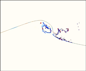
Sequences of three different plunging breakers with contours of the normalized velocity magnitude $(u,v)/c$ are shown in figure 5. For wave 1, the wave begins to break as the wave crest steepens and becomes multivalued at $t / t_0 = 3.19$. A curled jet is formed projecting ahead of the wave, and a high and flat interface accumulates at the rear side of the wave crest. The overturning jet develops further and impacts the wavefront, forming a closed cavity from the entrapped air at $t / t_0 = 4.25$. The phenomena of the breaking event from wave breaking and jet impact to splash-up formation among waves 1, 2 and 3 are quite similar. However, some differences exist at the rear side of the wave crest and regarding the size and shape of the closed cavity. Due to the highly unsteady and rapidly evolving breaking crest, determining the location and speed of the crest is challenging. Instead, the maximum horizontal particle velocity $u$ is used to analyse the speed evolution from incipient breaking to jet impact. Notably, the phase speed in shallow water $c$, calculated using linear wave theory, exhibits significant discrepancies when compared with the measured wave phase speed, which can be determined by the distance between two crests. These discrepancies may arise from the highly nonlinear and asymmetric wave profile, as well as the persistent motion of the wave plate during wave breaking. For simplicity, we continue to use the shallow water phase speed $c$ here. Prior to wave breaking, the maximum horizontal particle velocity is located at the wave crest. The green star in figure 5 indicates the position where the maximum horizontal particle velocity is located at that moment. As the wavefront approaches vertical, the particle velocities become almost horizontal with the order of the phase speed. The location of the maximum horizontal particle velocity then shifts downwards to the vertical plane along the longitudinal direction. At this stage, the maximum horizontal particle velocity begins to increase until the plunging jet impacts, reaching its maximum value at the top of the entrapped air cavity within the curling jet. For wave 1, the front face becomes nearly vertical at $t / t_0 = 3.19$, with a horizontal crest particle velocity of $u / c = 1.57$. Upon impact of the plunging jet at $t / t_0 = 4.25$, the horizontal crest particle velocity increases to $u / c = 1.99$, representing a 27 % increase. For wave 2 and wave 3, the front face becomes nearly vertical at $t / t_0 = 2.88$ and $t / t_0 = 4.51$, respectively, with velocity increases of 40 % and 14 % up to the impact of the plunging jet at $t / t_0 = 4.19$ and $t / t_0 = 5.63$, respectively.

Figure 5.

Evolution of the free surface for the three different plunging breakers, labelled with the normalized velocity vectors $(u,v)/c$. Panels (a,c,e) correspond to the time when the wavefront nears vertical, while (b,d, f) indicate the time when the plunging jet impacts the wavefront. The green star indicates the position where the maximum horizontal particle velocity is located at that moment.

The wave-breaking process is illustrated using wave 1 as a representative example. Figure 6 shows the normalized streamwise velocity $u/c$, vertical velocity $v/c$ and vorticity $\omega / \omega _0$ at different stages of wave overturning (figure 6a,d,g, $(t-{t_{im}}) / t_0 = -1$), jet impingement (figure 6b,e,h, $(t-{t_{im}}) / t_0 = 0$), and splash-up (figure 6c, f,i, $(t-{t_{im}}) / t_0 = 1$), where $t_{im}$ denotes the time when the plunging jet impacts the wavefront, and $\omega _0=\sqrt {g/d}$ represents a reference vorticity. Figure 6(a–c) presents the distribution of the streamwise velocity component, with the maximum values $u/c = 1.62$ (figure 6a) at the neck below the wave crest, 2.21 (figure 6b) at the impact point where the toe of the jet connects with the wavefront and 2.65 (figure 6c) near the tip of the splash-up. Combined with the distribution of the vertical velocity, the water–particle velocities of the wave crest are found to be approximately horizontal, as shown by PIV measurements of breaking waves by Perlin, He & Bernal (Reference Perlin, He and Bernal1996). The vertical asymmetry can be clearly observed from the distribution of the vertical velocity. Vortices are identified as concentrated at the free surface as the wave overturns, becoming more intense during cavity closure and subsequent splash-ups. Figure 7 illustrates the normalized streamwise velocity $u/c$, vertical velocity $v/c$ and vorticity $\omega / \omega _0$ during the late stage of wave breaking at $(t-{t_{im}}) / t_0 = 2$, 4 and 6. Notably, the highest streamwise velocity components are concentrated on the ruptured ligaments and ejected droplets resulting from the splash-ups, reaching a maximum value of $u/c = 2.65$, as depicted in figure 7(a–c). By examining the distribution of the vertical velocity component in figure 7(d–f), we can identify the location of the original wave crest, as well as the number and positioning of the primary splash-up processes, since the vertical velocity component $v/c$ equals zero at the positions of the original wave crest and impact point. As the wave experiences repetitive jet impacts and splash-ups, the wavefront interfaces become turbulent, resulting in irregular turbulent patches. Figure 7(g–i) demonstrates that the vortices do not interact with the bottom, suggesting that the wave depth does not significantly influence the turbulent clouds induced by wave breaking in our study.

Figure 6.

Detailed normalized streamwise velocity $u/c$ (a–c), vertical velocity $v/c$ (d–f) and vorticity $\omega / \omega _0$ (g–i) during wave overturning (a,d,g), $(t-{t_{im}}) / t_0 = -1$; jet impact (b,e,h), $(t-{t_{im}}) / t_0 = 0$; and splash-up (c,f,i), $(t-{t_{im}}) / t_0 = 1$.

Figure 7.

Detailed normalized streamwise velocity $u/c$, vertical velocity $v/c$ and vorticity $\omega / \omega _0$ in the late stage after wave breaking at $(t-{t_{im}}) / t_0 = 2$, 4 and 6.

4.2. Energy budget

This section investigates the temporal evolution of the energy input by the wave plate, energy loss during wave breaking and the corresponding dissipation rate. Before proceeding, we acknowledge the inherent 3-D nature of turbulence and the potential controversies surrounding the use of 2-D simulations. Although 2-D simulations may not fully capture the complexities of 3-D turbulence, they have been widely employed in studying breaking waves due to their ability to reproduce key features and capture the dominant mechanisms governing the breaking process. Specific aspects of breaking waves, such as wave overturning and energy evolution, have been found to yield valuable insights through 2-D simulations. Previous studies, such as Iafrati (Reference Iafrati2009), have indicated that the overturning of the jet and the initial jet impact are primarily 2-D processes. Moreover, the assumption of two-dimensionality is reasonable, particularly in the early stages after the onset of breaking, when large air bubbles are entrapped. The use of 2-D DNS has also proven effective in capturing the dissipative scales of the breaking wave process, as demonstrated by Deike et al. (Reference Deike, Popinet and Melville2015). The 3-D effects are expected to become significant only in the subsequent stage, where instabilities in the cross-direction strongly influence both the fragmentation process of the air cavity and the dynamics of large vortical structures. Figure 8(a–c) illustrate the energy evolution in the wave tank for each case. Initially, there is no energy in the system, but as the wave plate begins to move and interact with the water body, the generation of waves leads to a simultaneous increase in gravitational potential energy and kinetic energy. The total energy continues to increase until the moment when the plunging jet impacts the wavefront. For waves 1, 2 and 3, this occurs at $t / t_0 = 4.25$, 4.19 and 5.63, respectively. Prior to the jet impact, two visible energy transfers between kinetic and potential energy can be observed, resulting from wave steepening and the descent of the plunging jet. Figure 8(d–f) present the temporal evolution of the total mechanical energy starting from the initial jet impact for three different waves. The associated dissipation rate is also depicted using dashed lines. Examining wave 1 in figure 8(d), the energy dissipation rate remains relatively small and constant from the impact of the plunging jet until just before the first splash-up impact, occurring at approximately $(t-t_{im}) / t_0 = 1$. Subsequently, as the first splash-up and its associated shedding droplets collide with the water surface, the energy dissipation rate begins to increase. From $(t-t_{im}) / t_0 = 1$ onwards, the wavefront interface undergoes significant perturbations due to multiple jet impacts, splashing events and the formation of entrapped bubbles and ejected droplets. These breaking processes enhance energy transfer and dissipation, leading to a rapid increase in the energy dissipation rate and a continuous decay of the total mechanical energy. After $(t-t_{im}) / t_0 = 3$, as the wave becomes more turbulent, the dissipation rate reaches its maximum, entering a plateau that remains relatively constant until approximately $(t-t_{im}) / t_0 = 8$. Following the intense dissipation caused by turbulence, the dissipation rate starts to decrease at a constant rate, with a noticeable reduction observed at approximately $(t-t_{im}) / t_0 = 13$. A similar trend is observed in waves 2 and 3, with a weaker energy transfer and turbulence region due to wave breaking. Notably, all scales of the breaking wave, from energy dissipation to the formation and breakup of bubbles and droplets in a two-phase turbulent environment, must be resolved in order to accurately capture the physics of breaking waves. However, this is not feasible in 2-D DNSs. The energy dissipation rates presented in figure 8(d–f), which are based on the decay of the mechanical energy, were used as a way of determining the active breaking period. The natural end time of breaking is not immediately obvious, but examining the evolution of dissipation rates provides a way to identify the point at which the wave has stopped breaking. While our 2-D results on the energy budget and dissipation provide a brief overview of energy evolution during breaking and its associated causes from a 2-D perspective, some physical phenomena such as the rupture of the main air cavity cannot be represented due to the absence of 3-D information. Consequently, it is not advisable to extrapolate from these 2-D results to infer the complete physical processes occurring during breaking.

Figure 8.

The temporal evolution of the normalized energy per unit length $E_l/(\rho g d^3)$ for wave 1 (a), wave 2 (b) and wave 3 (c) from the initiation of wave plate motion until the moment of jet impact. The motion of the wave plate transfers energy to the stationary water column, resulting in the propagation of waves at a constant water depth. Jet impact occurs at $t / t_0 = 4.25$, 4.19 and 5.63 for waves 1, 2 and 3, respectively. Panels (d–f) present the normalized energy per unit length $E_l/(\rho g d^3)$ and the normalized energy dissipation rate per unit length $\epsilon _l/(\rho g^{3/2} d^{5/2})$ starting from the time of jet impact for the three different waves. The energy dissipation is enhanced upon the plunging jet striking the wavefront. The dissipation rate first increases and then remains relatively constant for a period. Subsequently, the energy dissipation rate starts to decline, marking the end of the active breaking stage. Three grey lines indicate specific time points at $(t-t_{im}) / t_0 = (1/(2f))/t_0$, $(1/f)/t_0$ and $(3/(2f))/t_0$.

5.1. Influence of the Bond number on the main cavity

In this section, the effect of dimensionless parameters responsible for the wave evolution and breaking characteristics on the geometry of the main cavity at impact is investigated.

The effect of the Reynolds number on the wave evolution is expected to be small before wave breaking, as the jet thickness is independent of the Reynolds number, and no apparent dependence of the cavity size on the Reynolds number is discovered (Iafrati Reference Iafrati2009; Mostert et al. Reference Mostert, Popinet and Deike2022). The Reynolds independence of the wave characteristics and main cavity features is checked by comparing the numerical results for distinct Reynolds numbers of $6 \times 10^4$ and $6 \times 10^5$ with experimental data. These findings confirm the results obtained previously by Iafrati (Reference Iafrati2009). The influence of the Reynolds number on the wave features is neglected in this study since it has been shown to be negligible at high Reynolds numbers in breaking waves. Since our 2-D simulation provides a reasonable estimate of the wave profile and the formation of a plunging jet, which is considered the laminar structure before jet impingement occurs, the effects of the Bond number on the evolution of the wave profile and breaking characteristics of plunging breakers are determined by examining extensive cases with a wide range of Bond numbers. The Bond number increases from $6000$ to $80\,000$ in increments of $2000$, while all other parameters remain constant. Note that $Bo=8600$ refers to the surface tension between air and water in the experiments. Previous studies have revealed that a larger value of $Bo$ results in greater separation between the wavelength and Hinze scale, necessitating the use of costly numerical resources if all scales are to be resolved (Wang, Yang & Stern Reference Wang, Yang and Stern2016). Our high-resolution meshes that benefit from adaptive mesh refinement criteria can resolve breakers with greater separation between length scales, allowing us to vary $Bo$ over a wide range. For instance, for $Bo = 80\,000$, the capillary length $l_c = \sqrt {d^2/Bo} = 0.884$ mm, and the capillary length relative to the smallest grid size $l_c /\varDelta \sim 5$ at $l_{max}=15$. A similar capillary length to the smallest grid size ratio was utilized in the 3-D wave breaking DNS of $Re = 100\,000$ and $Bo = 1000$ by Mostert et al. (Reference Mostert, Popinet and Deike2022). Additionally, a grid number of 6.4 was employed to represent the initial sheet for investigating the motion and stability of the edge of a liquid sheet in 2-D. A rim forms at the edge of the free end of the sheet, and a neck appears just behind the rim, resembling the phenomena observed in the stretching of the plunging jet (Fuster et al. Reference Fuster, Agbaglah, Josserand, Popinet and Zaleski2009). These applications suggest that the current grid resolution is adequate for capturing the formation and geometry of the plunging jet. In addition, a convergence study was conducted to assess the ability of our 2-D simulation to capture the formation and geometry of the plunging jet, considering three different $l_{max}$ values of 14, 15 and 16 for $Bo = 80\,000$. As shown in figure 9, we observe that the agreement between $l_{max} = 15$ and 16 is better than that between $l_{max} = 14$ and 15, and the results for $l_{max} = 15$ and 16 are nearly coincident. This suggests that $l_{max} = 15$ is sufficient for achieving grid convergence, even at relatively high Bond numbers. Figure 10 illustrates the evolution of the wave profile under various Bond numbers at $t / t_0 = 2.5$, 3.1, 3.8 and 4.1. Qualitatively, the wave profile evolution does not exhibit a significant influence of $Bo$. The impact of $Bo$ primarily manifests in the development of the plunging jet, which features a rounded edge due to capillary retraction (Fuster et al. Reference Fuster, Agbaglah, Josserand, Popinet and Zaleski2009). At $t / t_0 = 2.5$, the generated wave crest experiences the effects of surface tension, resulting in a bulge on the front face of the steepening wave crest. The inset of figure 10(a) reveals a smaller bulge with the increasing Bond number, accompanied by a slightly larger wave height prior to breaking. This behaviour indicates that surface tension induces capillary ripples on the forwards face of the wave, leading to a bulge on the water surface. Experimental studies by Perlin et al. (Reference Perlin, He and Bernal1996) captured the appearance of parasitic capillary waves on the upper section of the vertical wavefront, specifically along the highest elevations of the lower front face of the plunging wave. Moreover, Diorio, Liu & Duncan (Reference Diorio, Liu and Duncan2009) observed that the bulge and capillary waves on the crest-front faces of the spillers at breaking onset are self-similar, independent of the breaking-wave-generation mechanism. This geometric similarity is limited to the crest-front profiles of the spillers and is attributed to the crest flow being dominated by surface tension and gravity. For larger Bond numbers where the influence of surface tension is negligible, a smaller bulge is formed. The slopes of the free surface upstream of the toe and the curvature of the bulge appear to increase with surface tension. The profile shapes and trends depicted in figure 10(a) exhibit qualitative similarities to numerical simulations of deep-water plunging and spilling breakers reported by Perlin et al. (Reference Perlin, He and Bernal1996) and Diorio et al. (Reference Diorio, Liu and Duncan2009). However, the detailed quantitative characteristics of the capillary ripples are beyond the scope of this study and are not discussed here. At $t / t_0 = 3.1$ (figure 10b), as the horizontal asymmetry of the wave profile develops further, the edge of the bulge erupts from a point just forwards of the crest and becomes tangent to the wave direction, presenting different widths of the bulge due to different surface tensions. The bulge due to surface tension projects forwards and develops into a plunging jet at $t / t_0 = 3.8$ (figure 10c), and a thicker jet can be observed at a smaller Bond number, indicating that jet thickness is dependent on the Bond number due to capillary effects caused by surface tension. Figure 10(d) shows that at $t / t_0 = 4.1$, the plunging jets at $Bo = 6000$ and 8000 impact the rising wavefront, ingesting a tube of air, while the plunging jets at $Bo = 12\,000$ and 16 000 still need more time to form the cavity. As the Bond number increases, the instant at which the plunging jet impinges on the front of the wave is delayed, and the plunging jet becomes thinner and projects farther forwards ahead of the wave, entrapping more air into the wave. The cross-sectional shape of the air cavity is affected by surface tension. Increasing the effect of surface tension causes the plunging jet to thicken and reduces the volume of air entrapped at the jet impact. The geometric properties of the main cavity caused by plunging breakers are identified by New (Reference New1983), showing that the surface profiles underneath the overturning crest may be represented by an ellipse of axes ratio $\sqrt {3}$, with its major axis rotated at an angle of approximately $60^{\circ }$ to the horizontal. A similar shape can be confirmed in our cases as shown in figure 11. The vertical height of the main cavity $h_c$, calculated as $h_c = h - h_t$, is closely related to the size of the main cavity entrapped by the plunging jet, where $h$ is the breaking height and $h_t$ is the height from the breaking crest to the cavity top. The cross-sectional area of the initially ingested cavity in the breaking process can be estimated by applying the ellipse area formula $A = {\rm \pi}(h_c/\sin 60^{\circ })^2/4\sqrt {3}$, where $h_c$ is the vertical height of the main cavity. By normalizing the main cavity using the cross-sectional area $A_0$, we obtain $A/A_0 \propto (h_c/h)^2$. A new scaling regarding the cavity correction factor for the entrained cavity is proposed as $A/A_0 = ((h-{\rm \pi} l_c)/h)^2$ by Mostert et al. (Reference Mostert, Popinet and Deike2022), with very good agreement at high Bond numbers and weaker agreement at lower Bond numbers. This indicates that $h_c = h-{\rm \pi} l_c$, where $l_c$ is the capillary length. Similar scaling can be proposed, but a coefficient of 0.6 should be used to mediate the difference between the width of the jet and the breaking height when it exhibits a greater separation between the wave scale and capillary length due to the larger Bond number in the present work, which gives $A/A_0 = (0.6(h - {\rm \pi}lc)/h)^2$. Figure 12(a) illustrates the geometry of the main cavity when the plunging jet connects with the front of the wave at $t/t_0 = 4.32$. It is observed that the size of the main cavity appears to be independent of the surface tension when increasing the Bond number, indicating a convergence of the main cavity size as the Bond number increases. Figure 12(b) shows very good agreement between this scaling and the present DNS results. As previously stated, the wave jet becomes thinner and projects farther forwards ahead of the wave as the surface tension decreases. It exhibits a breaking height $h_0$ in the absence of surface tension, which represents the maximum value of all breaking heights when surface tension is considered. The decreased breaking height caused by the shortened project distance normalized by $d$ is proportional to the cube of the capillary length normalized by $d$, which gives $(h_0-h)/d \propto ({l_c}/d)^3$, as shown in figure 12(c), while $h_t$ remains constant under a distinct Bond number. Figure 12(d) shows the comparison of the numerical results of $h/d$ to the estimated values of $h/d$ calculated using $h_0/d - C(l_c/d)^3$ by the proposed power-law scaling, with $C$ being a proportionality constant.

Figure 9.

Evolution of the free surface, spanning from jet formation to jet impact, is examined with a time interval of $\Delta t / t_0 = 0.16$. A large Bond number of $80\,000$, which represents a significant scale separation, is used for grid convergence analysis. The comparison between $l_{max} = 15$ and 16 exhibits better agreement compared with that between $l_{max} = 14$ and 15, indicating that $l_{max} = 15$ adequately achieves grid convergence, even for relatively high Bond numbers.

Figure 10.

The spatial evolution of the free surface and the development of overturning jet for wave 1 at various Bond numbers when $t / t_0 = 2.5$ (a), 3.1 (b), 3.8 (c), 4.1 (d).

Figure 11.

Estimation of the breaking height $h$, which is the sum of the height from the breaking crest to the cavity top $h_t$ and the vertical height of the main cavity $h_c$. The main cavity size $A$ is assumed to be proportional to ${h_c}^2$, which can be normalized by $A_0 \propto h^2$, giving that $A/A_0 \propto (h_c/h)^2$.

Figure 12.

Estimation of the main cavity size and breaking height. (a) The geometry of the main cavity when the plunging jet connects with the front of the wave at $t/t_0 = 4.32$ under various Bond numbers. (b) Relationship between cavity area and Bond numbers. (c) Linear relationship between the decreased breaking height caused by shortened project distance and the capillary length, $(h_0-h)/d \propto ({l_c}/d)^3$. (d) A scaling to estimate the breaking height at different Bond numbers.

5.2. Breaking criteria

This section develops the relationship between wave parameters, i.e. maximum wave height before breaking $H$ [${\rm L}$], breaking-wave crest $H_b$ [${\rm L}$] of the plunging breaker, and the initial conditions used to generate waves in this study by numerical data fitting, following the above dimensional analysis as stated in (2.4) and (2.5):

(5.1)$$\begin{gather} \frac{H}{d} = f_H\left(Re, Bo, \frac{s}{d}, \frac{fd}{c}\right), \end{gather}$$

(5.2)$$\begin{gather}\frac{H_b}{d} = f_{H_b}\left(Re, Bo, \frac{s}{d}, \frac{fd}{c}\right). \end{gather}$$

As discussed in § 5.1, $Re$ and $Bo$ do not significantly influence the wave characteristics, so the wave is considered independent of $Re$ and $Bo$ when discussing the scaling of $H$ and $H_b$ to the initial conditions. Thus,

(5.3)$$\begin{gather} \frac{H}{d} = f_H\left(\frac{s}{d}, \frac{fd}{c}\right) \propto \left(\vphantom{\frac{fd}{c}}\frac{s}{d}\right)^{\alpha_H} \left(\frac{fd}{c}\right)^{\beta_H}, \end{gather}$$

(5.4)$$\begin{gather}\frac{H_b}{d} = f_{H_b}\left(\frac{s}{d}, \frac{fd}{c}\right) \propto \left(\vphantom{\frac{fd}{c}}\frac{s}{d}\right)^{\alpha_{H_b}} \left(\frac{fd}{c}\right)^{\beta_{H_b}}. \end{gather}$$

This dimensional analysis demonstrates the dependence of the wave characteristics on the dominant dimensionless variables derived from the initial conditions. Their quantitative relations are investigated by conducting various cases for different combinations of $s$, $f$ and $d$ to determine the corresponding coefficients in the dimensionless expressions.

First, the wave characteristics are estimated from the simplified theory for plane wavemakers. In shallow water, a simple theory for the generation of waves by wavemakers was proposed by Galvin (Reference Galvin1964), who reasoned that the water displaced by the wavemaker should be equal to the crest volume of the propagating waveform. As breaking waves are generated by a piston wavemaker with a stroke of $s$ over a constant water depth $d$, the volume of water displaced over a whole stroke is $sd$. If the resulting waves are vertically symmetric with one single crest before breaking, then the crest volume of the propagating waveforms in a wavelength is $\int _{0}^{L/2}(H/2)(1-\cos kx)\,\mathrm {d}\kern0.06em x=HL/4$, where $L$ is the wavelength and $k = 2 {\rm \pi}/ L$ is the wavenumber; equating the two volumes gives

(5.5)\begin{equation} sd = \frac{HL}{4}. \end{equation}

According to the dispersion relation of shallow-water waves, the wavelength is $L = T \sqrt {gd}$. Then the resulting connection between the wave height and the initial conditions of the wave plate can be expressed as

(5.6)\begin{equation} \frac{H}{d} = \frac{4 s}{T \sqrt{gd}}. \end{equation}

Notably, the wave parameters $H$, $L$ and $T$ in this expression are theoretical values and do not represent the real values in actual waves, which already break before forming a symmetrical waveform, but it provides us with a possible relationship that can be used to determine the fit to the numerical data.

Then, the scaling of the maximum wave height before breaking $H$ of the experimental waves generated by the wave plate is fitted through the numerical results under various initial conditions. It can be seen from (5.3) that $H/d \propto s^{\alpha _H} f^{\beta _H} d^{{\beta _H}/2 - \alpha _H} g^{-{\beta _H}/2}$, so $H \propto s^{\alpha _H} f^{\beta _H} d^{{\beta _H}/2 - \alpha _H + 1} g^{-{\beta _H}/2}$. At the same frequency $f$, numerical results show that $H/d \propto s d^{-1/2}$ and $H \propto s d^{1/2}$, so we have $\alpha _H = 1$ and $\beta _H = 1$; thus, it gives

(5.7)\begin{equation} \frac{H}{d} \propto \frac{sf}{\sqrt{gd}} \propto \frac{U_{max}}{c}, \end{equation}

where $U_{max} = s{{\rm \pi} }f$ is the maximum wave plate velocity and $c = \sqrt {gd}$ is the linear velocity. This is quite similar to the theoretical result proposed in (5.6). Furthermore, the scaling of the breaking-wave crest $H_b$ with the initial conditions is also fitted through the numerical results. Based on the same method of analysing the numerical data, the exponents in the power-law scaling can be determined as $\alpha _{H_b} = 2/3$ and $\beta _{H_b} = 1/3$; thus

(5.8)\begin{equation} \frac{H_b}{d} \propto \left(\vphantom{\frac{fd}{c}}\frac{s}{d}\right)^{2/3} \left(\frac{fd}{c}\right)^ {1/3}. \end{equation}

Figure 13(a,b) shows the relationship between the normalized maximum wave height before breaking $H/d$ and breaking-wave crest $H_b/d$ to the initial conditions. A linear correlation between the maximum wave height before breaking $H$ and the maximum wave plate speed $U_{max}$ is revealed, showing that the wave height increases as the maximum wave plate speed increases. As indicated in figure 13, the generated wave remains non-breaking for $H/d\le 0.65$. The breaking is of the spilling type for $0.65\ge H/d\le 0.80$, whereas it is of the plunging type for $H/d\ge 0.80$. The above results agree with the measurement performed by Li (Reference Li2017), who showed that the critical value for spilling and plunging waves is $H/d=0.80$. For plunging breakers, a linear correlation between breaking-wave crest $H_b$ and initial conditions is also proposed, which is in good agreement with the numerical results.

Figure 13.

Scaling for the maximum wave height before breaking (a) and breaking wave crest (b) with respect to the initial conditions. Normalized wave height from (5.3) with the parameters $\alpha _H = 1$ and $\beta _H = 1$. This indicates that the wave height normalized by the water depth is proportional to the maximum wave plate velocity normalized by the wave phase speed. (b) The normalized breaking wave crest from (5.4) with the parameters $\alpha _{H_b} = 2/3$ and $\beta _{H_b} = 1/3$. (c) Relationship between the maximum fluid particle velocity before jet impact and the maximum wave plate speed.

We also present the relationship between the maximum fluid particle velocity at the moment of jet impact and the initial conditions. Figure 13(c) demonstrates a generally linear dependence between $u_{max}/c$ and $U_{max}/c$, where lower values of $U_{max}/c$ tend to correspond to higher values of $u_{max}/c$, while larger values of $U_{max}/c$ result in lower values of $u_{max}/c$. Deviations from this linear dependence may be attributed to nonlinearity and asymmetry introduced by our wave-making method. Waves associated with larger $U_{max}/c$ break earlier, limiting the acceleration of water particles, whereas waves corresponding to smaller $U_{max}/c$ receive energy from the rear side of the wave crest. In addition, the shoaling effect induced by higher nonlinearity leads to an increase in wave height and a decrease in fluid particle velocity.

5.3. Energy dissipation due to breaking

The energy dissipation rate due to breaking can be defined as $\epsilon _l = \Delta E_m / \Delta t$, which is the average decrease in the conservative energy $E_m$ over the active breaking period $\Delta t$. Notably, different studies have adopted varying definitions for the active breaking period. For instance, in the laboratory measurements conducted by Drazen and Kirby (2008) on deep-water breaking due to dispersive focusing, the duration of the breaking event is determined by differencing the start and stop times of breaking from the spectrogram of the hydrophone signal. On the other hand, when considering breaking solitary waves on plane slopes in shallow water, Mostert & Deike (Reference Mostert and Deike2020) defined the active breaking period as commencing when the wave face becomes vertical and ending when the kinetic energy $E_k$ equals the potential energy $E_p$. This definition ensures that the contribution of bottom boundary layer friction during run-up is excluded from the calculation of the dissipation during breaking. In the current case, where the wave breaks due solely to nonlinearity in a tank with a level bottom, the dominant mechanism of dissipation comes from viscous dissipation by turbulence in the upper layers. If we assume that most of the viscous dissipation occurs while the wave is actively breaking, then the active breaking phase ends when the energy dissipation rate slows. As shown in figure 8(d–f), the energy dissipation rate initially exhibits a rapid increase with time, reaching its maximum at approximately $(t-t_{im}) / t_0 = (1/(2f))/t_0$. Subsequently, the dissipation rate remains relatively constant for a duration of $1/(2f)$, after which it begins to decay. A noticeable decay in the energy dissipation rate can be observed at approximately $(t-t_{im}) / t_0 = (3/(2f))/t_0$, which may indicate the end of the active breaking stage. Therefore, in this study, the active breaking period is defined as the period starting when the jet impacts and lasting $\Delta t = 3/(2f)$, once the quasiequilibrium stage has ended and the energy dissipation rate begins to decay.

The physical parameters for the energy budget are the total energy per unit length transferred by the motion of the wave plate $E_l$ [ML T$^{-2}$] and the energy dissipation per unit length of the wave crest $\epsilon _l$ [ML T$^{-3}$] for plunging breakers. Then, the dimensional analysis for the energy budget gives

(5.9)$$\begin{gather} \frac{E_l}{\rho g d^3} = f_{E_l}\left(Re, Bo, \frac{s}{d}, \frac{fd}{c}\right), \end{gather}$$

(5.10)$$\begin{gather}\frac{\epsilon_l}{\rho g^{3/2} d^{5/2}} = f_{\epsilon_l}\left(Re, Bo, \frac{s}{d}, \frac{fd}{c}\right). \end{gather}$$

Likewise, the energy budget is assumed to be independent of the Reynolds number and Bond number. Thus,

(5.11)$$\begin{gather} \frac{E_l}{\rho g d^3} = f_{E_l}\left(\frac{s}{d}, \frac{fd}{c}\right) \propto \left(\vphantom{\frac{fd}{c}}\frac{s}{d}\right)^{\alpha_{E_l}} \left(\frac{fd}{c}\right)^{\beta_{E_l}}, \end{gather}$$

(5.12)$$\begin{gather}\frac{\epsilon_l}{\rho g^{3/2} d^{5/2}} = f_{\epsilon_l}\left(\frac{s}{d}, \frac{fd}{c}\right) \propto \left(\vphantom{\frac{fd}{c}}\frac{s}{d}\right)^{\alpha_{\epsilon_l}} \left(\frac{fd}{c}\right)^{\beta_{\epsilon_l}}. \end{gather}$$

We first determine the relationship between the total energy per unit length and the initial conditions. According to linear wave theory, the total energy per wave unit width is given by $E_l = \rho g H^2 L / 8$. Thus, the dimensionless wave energy can be expressed as $E_l / (\rho g d^3) = H^2 L / (8 d^3)$. Assuming that the generated wave has the same frequency as the wave plate, we can calculate the nominal wavelength $L$ using the dispersion relationship in shallow water, i.e. $L = T \sqrt {gd} \propto \sqrt {gd} / f$. Furthermore, we have derived the scaling between wave height and the initial conditions as $H / d \propto sf / \sqrt {gd}$. Consequently, we find that $E_l / (\rho g d^3) = H^2 L / (8 d^3) \propto (s/d)^2 (fd/c)$. Therefore, the scaling of the energy budget with respect to the initial conditions is determined by $\alpha _{E_l} = 2$ and $\beta _{E_l} = 1$ and can be described as

(5.13)\begin{equation} \frac{E_l}{\rho g d^3} \propto \left(\vphantom{\frac{fd}{c}}\frac{s}{d}\right)^2 \left(\frac{fd}{c}\right). \end{equation}

Figure 14 shows the relationships between the total energy transferred by the motion of the wave plate $E_l$ and the initial conditions. It is evident that the measured total energy from the numerical data is generally in agreement with the estimated results from the initial conditions. However, in the lower range of total energy, which corresponds to lower nonlinearity, the estimated total energy derived from the initial conditions tends to underestimate the measured total energy.

Figure 14.

Scaling for the total energy transferred by the motion of wave plate $E_l$. Normalized total energy from (5.13) with the parameters $\alpha _{E_l} = 2$ and $\beta _{E_l} = 1$.

Next, we aim to establish a scaling relationship between the energy dissipation rate during wave breaking and the wave parameters. This scaling is based on an inertial model for estimating the energy dissipation rate, similar to the approach employed by Drazen et al. (Reference Drazen, Melville and Lenain2008) for deep-water breakers and Mostert & Deike (Reference Mostert and Deike2020) for shallow-water breakers. We seek to validate the applicability of this framework in predicting energy dissipation during breaking in shallow water over a flat-bed geometry. To establish a connection between the isotropic turbulence assumption and the empirical relationship, accurate estimations are required for the turbulent integral length scale $l$, the characteristic velocity scale $w$ and the turbulent cloud cross-section $A$. In the study by Drazen et al. (Reference Drazen, Melville and Lenain2008) on plunging breaking waves in deep water, an inertial model is employed to estimate the dissipation rate, using the local wave height $h$ and velocity at impact as the length and velocity scales, respectively. The trajectory of the toe, as measured in the experiment, indicates that the toe of the breaker is in freefall under gravity, descending a height $h$. Consequently, the vertical velocity of the toe at impact can be approximated as $w = \sqrt {2gh}$. By assuming a cylindrical cloud of turbulence of cross-sectional area $A = {\rm \pi}h^2 /4$ and applying the linear dispersion relationship in deep water, they argued that the breaking parameter $b$ should be proportional to $S^{5/2}$, where $S = hk$ is the local slope at breaking. Following the same inertial model, Mostert & Deike (Reference Mostert and Deike2020) quantified the energy dissipation caused by breaking solitary waves in shallow water on a gentle slope. They determined the impact velocity of the plunging jet as $w = \sqrt {2gH_b}$, where $H_b$ is the wave height at breaking. The turbulent integral length scale $l$ is estimated by the undisturbed depth at breaking $d_b$, as $d_b$ sets the upper limit on the size of eddies that form from the breaking process. This was corroborated by examining the vorticity in the liquid phase during the breaking event, which demonstrated that the mixing zone reaches the slope bed and is constrained by the depth. Utilizing the inertial model, they established a relationship between the dissipation resulting from wave breaking during the active breaking period and the local wave height, depth and beach slope, denoted as $b \propto (H_b/d_0)^{7/2}(d_b/d_0)^{-1}$, where $d_0$ is the water depth before the wave enters the slope. The same estimation method utilized by Mostert & Deike (Reference Mostert and Deike2020) can be applied to our breaking waves in shallow water. However, there are notable distinctions between our breaking waves and the wave breaking on a slope examined in their work. Unlike waves breaking on a slope, our waves propagate in a tank with a flat bottom and break due to strong nonlinearity. Although in many cases the breaking height $H_b$ exceeds the water depth $d$, since the plunging jet descends from a wave crest and impacts the wavefront, the mixing zone is situated near the initial water depth and is still bounded by the breaking height $H_b$. This can also be supported by the vorticity field during the postbreaking period, as depicted in figure 7. By considering a cylindrical cloud of turbulence with a cross-sectional area of $A = {\rm \pi}{H_b}^2 /4$, a vertical height of $H_b$ and an impact velocity of the toe $w = \sqrt {2gH_b}$, the dissipation per unit length along the wave crest is

(5.14)$$\begin{gather} \epsilon_l = \rho A \epsilon = \rho \frac{{\rm \pi} {H_b}^2}{4} \frac{\sqrt{2gH_b}^3}{H_b} \propto \rho g^{3/2} {H_b}^{5/2}, \end{gather}$$

(5.15)$$\begin{gather}b = \frac{\epsilon_l}{\rho {c}^5 / g} = \frac{\epsilon_l}{\rho g^{3/2} d^{5/2}} \propto \left(\frac{H_b}{d}\right)^{5/2}. \end{gather}$$

This scaling demonstrates that the dominant dimensionless variable describing the energy dissipation by breaking in shallow water is the ratio of $H_b$ and $d$. Multiple experimental measurements have demonstrated that energy dissipation associated with wave breaking exhibits a threshold dependence on $S$, with the dissipation rapidly approaching zero at low values of $S$. Drawing on laboratory data from various sources, Romero et al. (Reference Romero, Melville and Kleiss2012) proposed a semiempirical result by introducing a slope-based breaking threshold $S_0$, which can be expressed as $b = a(S - S_0)^n$, where $a$ is a constant and $S_0$ is a threshold slope for breaking. Based on a visual fit through the data, a power of $5/2$ consistent with the inertial scaling of Drazen et al. (Reference Drazen, Melville and Lenain2008), as well as a slope threshold of $S_0 = 0.08$ and a scaling factor of $a = 0.4$ were obtained. In the shallow-water cases, our numerical results also reveal a threshold behaviour in the energy dissipation associated with wave breaking. As shown in figure 15(a), the green dotted line represents a fit to the inertial scaling $b = a (H_b/d)^{5/2}$ with a coefficient value of $a = 0.06$. However, when the inertial scaling is extended to smaller values of $H_b/d$, it overestimates the dissipation rate compared with the numerical data. This discrepancy clearly indicates that the energy dissipation approaches zero at low values of $H_b/d$, exhibiting threshold behaviour. To account for this observation, we adopt a semiempirical scaling relationship of the form $b = a(H_b/d - \chi _0)^n$, where $\chi _0$ denotes the critical value for $H_b/d$. By fitting the numerical data, we can obtain the best-fitting parameters for this scaling relationship as

(5.16)\begin{equation} \frac{\epsilon_l}{\rho g^{3/2} d^{5/2}} = a\left(\frac{H_b}{d} - \chi_0\right)^n = 0.21\left(\frac{H_b}{d} - 0.65\right)^{1.5}. \end{equation}

This reveals a threshold value of $\chi _0 = 0.65$ and a power law scaling of $n = 1.5$. Figure 15(a) illustrates the fitted curve that smoothly connects all the numerical data. Notably, the obtained threshold $\chi _0$ closely aligns with the breaking criterion $H/d = 0.65$, which distinguishes between breaking and non-breaking waves. Note that this link between the energy dissipation rate and the local breaking parameters is applicable to plunging breakers. Although spilling waves exist within the $H_b/d$ range of 0.65–0.76, the dissipation associated with spilling breakers is not depicted in this context. The validation of the relationship between dissipation caused by spilling breakers and local breaking parameters would require additional data, but it exceeds the scope of this discussion. This critical value for $H_b/d$ can be justified by the absence of energy dissipation in non-breaking waves. It is worth highlighting that in deep water scenarios, the scatter of the data at high values of $S$ and the relatively small threshold slope $S_0$ allow for retaining the power law of $5/2$ in the inertial scaling proposed by Drazen et al. (Reference Drazen, Melville and Lenain2008) when the slope threshold is introduced. However, in shallow-water cases, the critical value $\chi _0 = 0.65$ significantly modifies the power law from the inertial scaling of $5/2$ to $1.5$. As stated in § 5.2, based on the relationship of the normalized breaking-wave crest to the initial conditions $H_b/d = 1.19(s/d)^{2/3}(fd / c)^{1/3}$, the energy dissipation rate can also be connected to the initial conditions. Figure 15(b) shows a good dependence between the energy dissipation rate and the initial conditions.

Figure 15.

Scaling for the energy dissipation per unit length of breaking wave $\epsilon _l$ (a) with respect to the initial conditions. (a) Scaling for energy dissipation per unit length of breaking wave $\epsilon _l$ with respect to local breaking parameters $H_b/d$, as shown in (5.16). (b) Normalized energy dissipation rate based on the relationship between the breaking wave crest $H_b/d$ and the initial conditions.

Based on the aforementioned analysis, the magnitude of the breaking parameter $b$ in shallow-water breaking waves is influenced by the ratio of the local breaking crest height to the water depth, highlighting the significant role of water depth in energy dissipation in shallow water. The breaking parameter $b$ exhibits a threshold dependence on $H_b/d$, rapidly tending to zero for low values of $H_b/d$. As $H_b/d$ increases, the breaking parameter asymptotically converges to the inertial scaling of $5/2$. These findings, which combine a local inertial turbulent argument and empirical results through least squares fit to the numerical data, establish a relationship between the dissipation rate and wave parameters, providing predictive insights into the dissipation rate of breaking waves in shallow water.

A comparative analysis was conducted using data from the literature in both deep water (sourced from Deike (Reference Deike2022)) and shallow water (sourced from Boswell et al. (Reference Boswell, Yan and Mostert2023)) conditions. As originally proposed by Beji (Reference Beji1995) and subsequently applied in the numerical investigation conducted by Boswell et al. (Reference Boswell, Yan and Mostert2023), a nonlinearity parameter $F = ga/c^2$ was used to connect the two distinct regimes, where $a$ is a representative amplitude and $c$ is a phase speed. In deep water, where $c = \sqrt {g/k}$, the nonlinearity parameter $F \sim ak = S$ corresponds to the wave slope, while it converges to $a/d$ in shallow water, with $c = \sqrt {gd}$. In our cases, $F$ approaches $H_b/d$ as $a \sim H_b$. Figure 16 shows the breaking parameter $b$ for deep-water breakers from a variety of experimental and numerical sources (Kendall Melville Reference Kendall Melville1994; Banner & Peirson Reference Banner and Peirson2007; Drazen et al. Reference Drazen, Melville and Lenain2008; Grare et al. Reference Grare, Peirson, Branger, Walker, Giovanangeli and Makin2013; Deike et al. Reference Deike, Popinet and Melville2015, Reference Deike, Melville and Popinet2016; Derakhti & Kirby Reference Derakhti and Kirby2016; De Vita et al. Reference De Vita, Verzicco and Iafrati2018; Mostert et al. Reference Mostert, Popinet and Deike2022), along with the shallow-water dataset from Boswell et al. (Reference Boswell, Yan and Mostert2023) and the present study. The breaking dissipation in this study falls between the previously established deep-water regimes and the shallow-water breaking waves documented by Boswell et al. (Reference Boswell, Yan and Mostert2023), and shows favourable consistency within the range of overlap between our data and Boswell's data. Furthermore, our data extend the left-hand boundary of this range by extending the nonlinearity parameter, specifically, $H_b/d$ from 0.85 to 0.75. This particular range displays a discernible diminishing trend in the breaking parameter $b$ as the nonlinearity parameter $F$ decreases. A similar trend can also be observed in Boswell's data. However, there is a clear discontinuity between the deep-water and shallow-water regimes, rendering a single power-law scaling inadequate for capturing both datasets. As introduced by Romero et al. (Reference Romero, Melville and Kleiss2012), a heuristic examination of the breaking threshold was undertaken to fit the extensive experimental and numerical observations in deep-water scenarios, yielding a semiempirical formulation $b = 0.4(S - 0.08)^{5/2}$, where $S \sim F$ under deep-water conditions. Notably, Boswell et al. (Reference Boswell, Yan and Mostert2023) made a commendable effort to address the discontinuity across various depth regimes using the same concept of breaking threshold dependence, and a slope threshold $F* = 0.7$ was determined in Boswell's shallow-water solitary wave cases. In our cases, the critical breaking threshold $F*$ was determined to be 0.65 through the best fit to our numerical data. The expression $b = 0.212(F - 0.65)^{1.5}$ collapses the DNS data presented in the present study favourably. However, the proposed semiempirical scaling fails to encompass the DNS data of shallow-water solitary breaking waves from Boswell et al. (Reference Boswell, Yan and Mostert2023). Therefore, further endeavours should be made to develop a comprehensive breaking parametrization. Nevertheless, the available datasets summarized in figure 16 offer valuable insights into this unsolved problem. The data suggest the possibility of a varying breaking threshold, particularly in the context of transitioning between deep and shallow water conditions. A determination relation governing the breaking threshold could be proposed to accommodate the different depth regimes. This remains to be explored in future work.

Figure 16.

Energy dissipation from laboratory experiments and numerical simulations: DW, deep water; SW, shallow water. The solid line is the semiempirical formulation in deep water regimes, $b = 0.4(F - 0.08)^{5/2}$ (Romero et al. Reference Romero, Melville and Kleiss2012), with breaking threshold $F*=0.08$, while the dotted line is the semiempirical formulation in deep water regimes proposed by Boswell et al. (Reference Boswell, Yan and Mostert2023) with $F*=0.65$. The dashed line is a visual fit through the present data, giving $b = 0.212(F - 0.65)^{1.5}$. THL, Tainan Hydraulics Laboratory wave tank; SIO, Scripps Institution of Oceanography wave tank; DNS, direct numerical simulations; LES, large eddy simulations.