


1. Introduction
The interaction of sea surface waves with natural and artificial marine structures lends itself to a wealth of analytical and numerical models (Faltinsen Reference Faltinsen1993; Linton & McIver Reference Linton and McIver2001; Mei, Stiassnie & Yue Reference Mei, Stiassnie and Yue2005; Folley Reference Folley2016). Intensive computations, such as those required for structure optimisation or for the determination of long-term force and motion statistics, together with the need for intelligibility and analytical tractability, call for relatively simple models, whereby wave force calculations and the structure dynamics are based on linear hydrodynamic theory, and extensions thereof through additional modelling terms. Such models are essential tools in the design and optimisation of ships, offshore structures, etc. – without negating the importance of more realistic numerical models to study specific events.
For structures of characteristic dimension small with respect to wavelength, and comparable to or smaller than the wave amplitude, wave forces are dominated by inertial terms (i.e. the dynamic pressure forces due to the incident, undisturbed flow, also termed Froude–Krylov forces, together with added-mass terms) and drag terms (i.e. due to flow separation) (Mei et al. Reference Mei, Stiassnie and Yue2005). Slender structures (Luhar, Infantes & Nepf Reference Luhar, Infantes and Nepf2017) and small surface scatterers (Garnaud & Mei Reference Garnaud and Mei2010) belong to this category. In contrast, for structures with characteristic size comparable to or larger than the wavelength and wave height, diffraction forces (i.e. due to the flow modification induced by the presence of the solid body) dominate. Between those two archetypal scenarios, there exist more nuanced cases where inertia is significant, alone or in combination with diffraction, and cases where the three types of forces should be modelled. Those different wave force regimes are depicted in the diagram of figure 1, reproduced from Chakrabarti (Reference Chakrabarti1987).

Figure 1. Different wave force regimes (Chakrabarti Reference Chakrabarti1987), as reproduced from Negro et al. (Reference Negro, López-Gutiérrez, Dolores Esteban and Matutano2014). For structures of characteristic dimension small with respect to wavelength ( ${\rm \pi} D/\lambda \ll 1$), and comparable to or smaller than the wave amplitude ( $H/D\geq 1$), wave forces are dominated by inertial and drag terms. For structures with characteristic size comparable to or larger than the wavelength ( ${\rm \pi} D/\lambda \geq 1$) and wave height ( $H/D\leq 1$), diffraction forces dominate. Between those two archetypal scenarios, there exist more nuanced cases.
In drag- and inertia-dominated situations, the effect of the structure on the wave field is assumed negligible, and one is therefore primarily interested in the structure forces or motion, rather than in the flow. Hydrodynamic forces are typically modelled as a quadratic damping drag term and a linear inertial term (Morison, Johnson & Schaaf Reference Morison, Johnson and Schaaf1950). The damping term is similar in form to the force used for constant flows, with a different coefficient, which accounts for the oscillatory nature of the flow (Keulegan & Carpenter Reference Keulegan and Carpenter1956). Such formulations are convenient, since they are not difficult to compute in numerical simulations, and they encapsulate the nonlinear nature of drag-induced forces, which increase more than linearly with the amplitude of the relative flow velocity. However, they do not indicate how the wave field is modified. In many cases, however, the effect on the wave field is also important to examine, when collective effects enter into account (seagrass, arrays of cylinders or other wave-dissipating structures Garnaud & Mei Reference Garnaud and Mei2010; Luhar et al. Reference Luhar, Infantes and Nepf2017; Nové-Josserand, Godoy-Diana & Thiria Reference Nové-Josserand, Godoy-Diana and Thiria2019), or when the motion of the structures is such that a significant fraction of the wave energy can be absorbed or dissipated, in spite of the small structure dimension, as is often the case for ‘point-absorber’ wave energy converters (Budal & Falnes Reference Budal and Falnes1975).
When diffraction is dominant, the effect of the structures on the wave field is duly represented in linear hydrodynamic models. However, even diffraction-dominated structures may require the inclusion of drag-induced terms, at least to avoid unrealistically large predictions of the structure or fluid motion, for example around the resonant frequency of a floating structure or for particular fluid modes. Drag forces are especially important when the wave energy budget is of interest, in particular for diffraction-dominated wave energy converters such as the large, flap-like devices known as ‘oscillating wave surge converters’ (Cummins & Dias Reference Cummins and Dias2017), or for coastal protection devices such as breakwaters. In such cases, consistently with the additional quadratic force formulation, vortices lead to a loss of energy, that should be (physically) subtracted from the wave field. To our knowledge, this effect has not been taken into account in the numerical modelling of wave energy arrays (Folley Reference Folley2016; Verbrugghe et al. Reference Verbrugghe, Stratigaki, Troch, Rabussier and Kortenhaus2017; Vervaet et al. Reference Vervaet, Stratigaki, De Backer, Stockman, Vantorre and Troch2022).
In short, there are a variety of situations where it is important to model accurately both the diffraction effect of structures on the wave field, together with drag-induced forces and the resulting flow modifications. In those situations, drag-induced dissipation should reduce the amplitude of the waves that are diffracted and radiated to the far field, while, in return, wave diffraction or radiation by the structures modify the flow locally, thus making the pertinent relative velocity different from that of the incident flow, which should alter drag-induced dissipation. This relation between the far-field and locally dissipated energy is seldom articulated in hydrodynamic models. A notable exception concerns the study of slotted barriers (Bennett, McIver & Smallman Reference Bennett, McIver and Smallman1992; Isaacson, Premasiri & Yang Reference Isaacson, Premasiri and Yang1998), porous screens and media (Arnaud et al. Reference Arnaud, Rey, Touboul, Sous, Molin and Gouaud2017; Mackay & Johanning Reference Mackay and Johanning2020) and other breakwater-like devices, designed at reflecting and dissipating a significant fraction of the incident wave energy. Concerning the hydrodynamics of rigid, impermeable bodies, where dissipation mostly occurs near corners and sharp edges, the authors of the present study have not been able to find any study which indicates how vortex shedding affects the far-field flow. At best, based on experimental data, a couple of studies limit themselves to noting that drag-dissipated energy seems to be removed from the transmitted, rather than the reflected, wave (Knott & Mackley Reference Knott and Mackley1980; Stiassnie, Naheer & Boguslavsky Reference Stiassnie, Naheer and Boguslavsky1984).
In this article, we highlight experimentally the importance of the interplay between wave diffraction, on the one hand, and drag-induced forces and dissipation, on the other hand, and we suggest modelling approaches which encapsulate it. To do so, we consider the simple case of wave diffraction by a vertical plate in a channel, which is equivalent to an infinite row of fixed vertical structures parallel to the wave front. In such a set-up, the far-field representation reduces to incident, reflected and transmitted waves, which greatly simplifies the analysis. In particular, we shall make use of the geometrical framework proposed by Mérigaud, Thiria & Godoy-Diana (Reference Mérigaud, Thiria and Godoy-Diana2023), which consists of representing the transmission coefficient in the complex plane, and allows for a straightforward visualisation of the energy budget between reflected waves, transmitted waves and power dissipation near the structure.
The remainder of this article is organised as follows: in § 2, linear potential flow theory is used to model the diffraction problem, and the inclusion of drag-induced dissipation and forces within this modelling framework is discussed, while the details of the mathematical and numerical solution are left to Appendix A. Based on a geometrical representation, § 3 discusses how the far-field flow (that is, reflected and transmitted waves) may be modified in the presence of drag-induced dissipation, and explores the connection between wave reflection and the hydrodynamic forces exerted onto the structure. In § 4, the application of the more usual Morison drag force model is detailed for our case study. Section 5, complemented with Appendix B, introduces the experimental set-up and procedure, and § 6 shows the experimental results, compared with their numerical counterparts. Finally, conclusions and avenues for future work are outlined in § 7.
2. Potential flow model and numerical solution
2.1. Linear potential flow model
A vertical, rigid, rectangular plate is located in the middle of a channel of width  $W$, filled with water. The plate extends vertically throughout the whole water depth $h$, assumed constant, laterally over a width $w$, and it is considered infinitely thin. The origin of the Cartesian frame is chosen to be the middle of the channel, at the bottom of the barrier; $x$,
$x$,  $y$ and $z$ represent the longitudinal, lateral and vertical position coordinates, respectively. The problem geometry and notations are summarised in figure 2.

Figure 2. Problem geometry and main notations: (a) side view, (b) front view. A vertical, rigid, rectangular plate of width  $w$ is located in the middle of a wave channel of width $W$ and depth $h$. The flow is described through linear potential theory. The incident wave, represented by the incident potential flow $\phi _I$, impinges upon the barrier. The scattered flow is denoted as $\phi _-$ in the up-wave zone, and $\phi _+$ in the down-wave zone.
The fluid is assumed inviscid, incompressible and the flow irrotational. The flow can thus be described through potential flow theory whereby, everywhere, the flow local velocity vector  $\boldsymbol {u}$ is calculated from the potential function $\phi (x, y,z,t)$ as
 \begin{equation} \boldsymbol{u} = \boldsymbol{\nabla} \phi. \end{equation}
Small perturbations are assumed, so that linear potential theory can be employed throughout. The potential satisfies the Laplace equation within the fluid domain, which reads
 \begin{equation} \nabla^2\phi = 0, \end{equation}
together with boundary conditions. The kinematic-dynamic boundary condition at the free surface reads
 \begin{equation} \frac{\partial^2 \phi}{\partial t^2} + g\frac{\partial \phi}{\partial z} = 0 \quad \text{in } z = h, \end{equation}
where  $g$ is the gravity constant.
No-flow conditions hold on solid boundaries, i.e. at the sea bottom
 \begin{equation} \frac{\partial \phi}{\partial z} = 0 \quad \text{in } z = 0, \end{equation}
at the vertical lateral walls
 \begin{equation} \frac{\partial \phi}{\partial y} = 0 \quad\text{in } y ={\pm} W/2 \end{equation}
and on the two sides of the vertical barrier
 \begin{equation} \frac{\partial \phi}{\partial x} = 0 \quad\text{in } x = 0^+_-,\quad |y| \leq w/2. \end{equation}
 A harmonic incident wave with frequency  $\omega$ travels forward along the channel. Using the problem linearity, in steady state, all quantities can be defined harmonically. In particular, the potential, dynamic pressure, flow velocity and free-surface elevation are defined from spatial complex functions $\hat {\phi }(x,y,z)$, $\hat {p}(x,y,z)$, $\hat {\boldsymbol {u}}(x,y,z)$ and $\hat {\eta }(x,y)$ as
 \begin{equation} \begin{cases} \phi(x,y,z,t) = {\rm Re} \{\hat{\phi}(x,y,z) {\rm e}^{-{\rm i}\omega t}\} \\ p(x,y,z,t) = {\rm Re} \{\hat{p}(x,y,z) {\rm e}^{-{\rm i}\omega t}\} \\ \boldsymbol{u}(x,y,z,t) = {\rm Re} \{\hat{\boldsymbol{u}}(x,y,z) {\rm e}^{-{\rm i}\omega t}\}\\ \eta(x,y,t) = {\rm Re} \{\hat{\eta}(x,y) {\rm e}^{-{\rm i}\omega t}\}. \end{cases} \end{equation}
2.2. Introducing drag-induced dissipation to the potential solution
Although the incident wave amplitude may be smaller than the obstacle characteristic dimension  $w$, the singularities at the sharp edges of the thin barrier result in a locally large flow velocity, thus inducing flow separation and vortices, which cannot be represented in a potential flow framework. We therefore adopt an approach similar to that of Cummins & Dias (Reference Cummins and Dias2017), which consists of introducing a porous-wall condition across a virtual dissipative surface near the edges of the barrier, where vortices are known to occur. Such conditions at an interface are commonplace in the modelling of breakwaters, porous screens or slotted structures (Bennett et al. Reference Bennett, McIver and Smallman1992; Isaacson et al. Reference Isaacson, Premasiri and Yang1998; Mackay & Johanning Reference Mackay and Johanning2020), where they allow the determination of the structure reflection and transmission coefficients. Only more recently have they been proposed for impermeable bodies, with the different aim of preventing the calculation of unrealistic spikes in the hydrodynamic response of oscillating structures or fluid modes (Chen, Duan & Liu Reference Chen, Duan and Liu2011; Cummins & Dias Reference Cummins and Dias2017; Feng, Chen & Dias Reference Feng, Chen and Dias2018).
In the work of Cummins & Dias (Reference Cummins and Dias2017), the virtual surface has two parameters, which should both be calibrated experimentally, namely a dissipation coefficient, and the width of the virtual surface where dissipation is expected to take place. Note, however, that this is only one of many possibilities to introduce dissipation on the virtual surface. It could be imagined, for example, that the porosity properties instead change gradually according to some continuous profile. Such an idea is detailed further in Appendix A.
In this work, we simplify the model by extending the width of the virtual porous screen to the whole gap between the barrier edge and the channel lateral wall (i.e.  $w/2 \leq |y| \leq W/2$), so that only the porosity coefficient needs to be tuned. In addition, the pressure drop at the interface is expressed as a quadratic function of the local flow velocity. In spite of the chosen homogeneous porosity profile, because of the quadratic pressure drop, energy dissipation increases cubically with the local flow velocity, so that the model should predict energy dissipation occurring predominantly in the vicinity of the barrier edge singularity, where the local flow velocity grows to infinity.
In mathematical terms, the porous-wall condition implies that the  $x$-wise velocity is continuous, while the drop in dynamic pressure $p = -\rho ({\partial \phi }/{\partial t})$ is expressed as
 \begin{equation} -\rho\left[\frac{\partial \phi_+}{\partial t} - \frac{\partial \phi_-}{\partial t}\right] = -\frac{1}{2}\rho \epsilon_q |\boldsymbol{\nabla} \phi|^2 \,\text{sign}\left(\frac{\partial \phi}{\partial x}\right), \end{equation}
where  $\epsilon _q$ is a non-dimensional parameter to identify from our experiments. In this way, the instantaneous dissipated power $P = \frac {1}{2} \rho \epsilon _q |{\partial \phi }/{\partial x}||\boldsymbol {\nabla } \phi |^2$ is proportional to the flux of kinetic energy across the virtual surface.
For the problem to be solved numerically, we need to linearise condition (2.8), as
 \begin{equation} -\rho\left[\frac{\partial \phi_+}{\partial t} - \frac{\partial \phi_-}{\partial t}\right] = -\rho \frac{g}{\omega} \epsilon_l \frac{\partial \phi}{\partial x}, \end{equation}
where  $\epsilon _l$ is found according to the Lorentz linearisation principle, i.e. such that the dissipated power is equal for both quadratic and linear pressure drop formulations. The latter condition reads $P_l(\epsilon _l) = P_q(\epsilon _l)$, where the ‘linear-case’ and ‘quadratic-case’ dissipated power values are given as follows:
 \begin{equation} \begin{cases} P_l(\epsilon_l) = \dfrac{1}{T}\rho \epsilon_l \dfrac{g}{\omega}\displaystyle\int_{0}^T\int_{0}^h \displaystyle\int_{ -W/2}^{W/2} \left|\dfrac{\partial \phi_{\epsilon_l}}{\partial x}\right|^2 |\hat{\eta}_I|^2 \, \mathrm{d}y\, \mathrm{d} z\, \mathrm{d} t \\[10pt] P_q(\epsilon_l) = \dfrac{1}{T}\dfrac{1}{2}\rho \epsilon_q \displaystyle\int_{0}^T\displaystyle\int_{0}^h \displaystyle\int_{ -W/2}^{W/2} |\boldsymbol{\nabla} \phi_{\epsilon_l}|^2 \left|\dfrac{\partial \phi_{\epsilon_l}}{\partial x}\right| |\hat{\eta}_I|^3 \,\mathrm{d}y\, \mathrm{d} z\, \mathrm{d} t, \end{cases} \end{equation}
where  $\phi _{\epsilon _l}$ is the potential per unit incident wave amplitude, obtained from the linear problem with condition (2.9), and $\hat {\eta }_I$ is the complex incident wave amplitude.
The quadratic loss coefficient  $\epsilon _q$ could be finely tuned based on experimental data. However, in this article, the choice is made to set this coefficient to a constant value of 1 throughout all wave frequencies, amplitudes and barrier dimensions, which amounts to stating that the energy, dissipated by the vortices during every half-wave cycle, equals the flux of kinetic energy through the interface during the same period of time. As shall be seen in § 6, even such a simple approximation gives satisfactory agreement with experimental data across the range of test conditions.
2.3. Numerical solution
Wave diffraction by a vertical barrier in a channel is a well-known hydrodynamic problem, which can be efficiently solved using matched eigenfunction expansion methods, as in Dalrymple & Martin (Reference Dalrymple and Martin1990). The approach of Dalrymple & Martin (Reference Dalrymple and Martin1990) is extended, by Wang et al. (Reference Wang, Qiu, Ye and Liang2016), to the solution of the radiation problem for oscillating wave surge converters (i.e. when the vertical barrier is able to pitch). In this work, we introduce minor generalisations of Dalrymple & Martin (Reference Dalrymple and Martin1990) and Wang et al. (Reference Wang, Qiu, Ye and Liang2016), namely by allowing the vertical structure to undergo arbitrary deflection modes, and by defining an arbitrary matching profile which accommodates, in a unified formulation, solid-wall, porous-wall and continuity conditions, across the interface of the vertical barrier plane. The mathematical and numerical details of the solution method are provided in Appendix A.
3. Far-field solution and hydrodynamic forces
3.1. Effect of drag on the far field
Assuming that the wave frequency is below the channel cutoff frequency (that is, the wavelength is larger than  $W$), the far-field scattered solution reduces to a transmitted plane wave and a reflected plane wave. Complex coefficients of reflection $\hat {R}$ and transmission $\hat {T}$ can thus be defined, which account for both a change in amplitude and a phase shift. In this section, we explain how transmission and reflection coefficients can be used to summarise and understand the main outcomes of the wave–structure interaction.
To do so, we adopt the geometric representation of reflection and transmission coefficients proposed by Mérigaud, Thiria & Godoy-Diana (Reference Mérigaud, Thiria and Godoy-Diana2021) and further generalised and detailed by Mérigaud et al. (Reference Mérigaud, Thiria and Godoy-Diana2023). Since the barrier is infinitely thin, it can be shown (Mérigaud et al. Reference Mérigaud, Thiria and Godoy-Diana2021) that
 \begin{equation} \hat{R}+\hat{T} = 1. \end{equation}
Thus, it suffices to represent  $\hat {T}$ to also represent $\hat {R}$, which can be read as $1-\hat {T}$. Note that, for other shapes of obstacles, one would still have the property $|\hat {R}+\hat {T}| = 1$ (Mérigaud et al. Reference Mérigaud, Thiria and Godoy-Diana2023).
Without dissipation, the incident wave energy is preserved in transmitted and reflected waves, which translates mathematically as  $|\hat {R}|^2 + |\hat {T}|^2 = 1$. Combined with (3.1), this ensures that $\hat {T}$ is located on a circle with centre $( 1/2, 0)$ and radius $1/2$, as exemplified in figure 3 through the case labelled ${\unicode{x24EA}}$. When dissipation is introduced, as explained in § 2.2, or as will be the case with physical experiments, the sum of transmitted and reflected energy coefficients decreases below unity, and the transmission coefficient location thus moves towards the interior of the circle, as in cases ${\unicode{x2460}}$, ${\unicode{x2461}}$ and ${\unicode{x2462}}$ of figure 3. More precisely, the dissipated power $P_d$, relative to the incident wave power $P_{wave}$, can be read through the distance $r$ from $\hat {T}$ to the centre $(1/2, 0)$, as $P_d/P_{wave} = 2(1/4-r^2)$ (Mérigaud et al. Reference Mérigaud, Thiria and Godoy-Diana2023).

Figure 3. Transmission and reflection coefficients  $\hat {T}$ and $\hat {R}$ represented in the complex plane, in a dissipation-free scenario ${\unicode{x24EA}}$ and in three possible dissipative scenarios ${\unicode{x2460}}$, ${\unicode{x2461}}$ and ${\unicode{x2462}}$. ${\unicode{x2460}}$ Assumes that only $\hat {T}$ is affected by dissipation, ${\unicode{x2461}}$ assumes that only $\hat {R}$ is affected, while ${\unicode{x2462}}$ assumes an intermediate situation.
As explained in the introduction, one of the primary objectives of this work is to study how drag-induced dissipation affects the far-field solution. Using the proposed geometric approach allows a straightforward visualisation of whether transmission, reflection or both, are modified by introducing drag, as illustrated in figure 3. In the figure, cases  ${\unicode{x2460}}$, ${\unicode{x2461}}$ and ${\unicode{x2462}}$ outline different possible hypotheses regarding the far-field modification due to drag: in case ${\unicode{x2460}}$, only transmitted energy decreases, leaving the reflection coefficient magnitude unchanged, in case ${\unicode{x2461}}$, on the contrary, only reflected energy decreases, while case ${\unicode{x2462}}$ represents an intermediate scenario.
3.2. Hydrodynamic forces and reflection coefficients
In this subsection, a linear potential flow solution is assumed, as in § 2. Consider  $\zeta (z)$ the deflection profile of the vertical barrier in the $x$ direction (in this case, a small rotation around its hinge axis), and $\hat {p} = {\rm i} \omega \rho \hat {\phi }$ the dynamic pressure from the potential solution $\hat {\phi }$ for a unit amplitude incident wave. With an incident wave with amplitude $\hat {\eta }_I$, the hydrodynamic force due to the unsteady pressure can be calculated as
 \begin{equation} \hat{f}_h = \hat{e} \hat{\eta}_I, \end{equation}
where the excitation force coefficient  $\hat {e}$ is calculated as follows:
 \begin{equation} \hat{e} = \int_0^h\int_{ -W/2}^{W/2} \zeta(z) [\hat{p}^-(y,z) - \hat{p}^+(y,z)] \,\mathrm{d}y \,\mathrm{d}z. \end{equation}
 When no dissipation occurs, as is usually the case in the linear hydrodynamics of impermeable bodies, the pressure continuity in the gap between the barrier and the wall ensures that the integral contribution for  $|y|>w/2$ is zero in (3.3). We denote as $\hat {e}_0$ the excitation coefficient obtained at a given frequency, assuming no dissipation.
Let us now consider the modified potential flow solution, with a pressure drop at the interface, as detailed in § 2.2. Applying (3.3) results in a generalised excitation force coefficient  $\hat {e}$, different from that of the dissipation-free case $\hat {e}_0$. In particular, with the virtual porous surface, the pressure contribution for $|y|>w/2$ is no longer zero. The difference with respect to $\hat {e}_0$ can thus be interpreted as the linearised drag force coefficient, $\hat {e}_d = \hat {e}-\hat {e}_0$. The total hydrodynamic force can now be further detailed as
 \begin{equation} \hat{f}_h = \hat{f}_0 + \hat{f}_{d,l}, \end{equation}
with  $\hat {f}_0 = \hat {e}_0 \hat {\eta }_I$ the traditional (dissipation-free) excitation force, and $\hat {f}_{d,l} = \hat {e}_d \hat {\eta }_I$ the drag force.
There exists a direct mathematical connection between the far-field solution and the excitation force. More specifically, it can be shown, see (A30), that
 \begin{equation} \hat{e} = 2 \rho g W \gamma_0 \hat{R}, \end{equation}
where  $\gamma _0$ denotes the projection of the deflection profile onto the first fluid vertical eigenmode, defined in (A27).
Thus, the coefficient  $\hat {R}$, as visualised in the complex plane according to our proposed geometrical framework, indirectly represents both the magnitude and the phase of the generalised excitation force coefficient. Figure 4 illustrates how the connection between hydrodynamic forces and reflection coefficients can be employed, to infer the complex drag force coefficient from reflection measurements. By considering the difference, in $\hat {R}$, between the dissipation-free ${\unicode{x24EA}}$ and dissipative ${\unicode{x2460}}$ cases, i.e. using $\hat {R}_d = \hat {R}_1 - \hat {R}_0$, the linearised drag force can be inferred using (3.5)
 \begin{equation} \hat{f}_{d,l} = \hat{e}_{d} \hat{\eta}_{I}, \end{equation}
with
 \begin{equation} \hat{e}_{d} = 2 g \rho W \gamma_0 \hat{R}_d. \end{equation}
Figure 4. Transmission and reflection coefficients  $\hat {T}$ and $\hat {R}$ represented in the complex plane, in a dissipation-free scenario ${\unicode{x24EA}}$ and in a dissipative scenario ${\unicode{x2460}}$. The reflection coefficient $\hat {R}_1$ can be decomposed into a dissipation-free component $\hat {R}_0$, related to the linear excitation force coefficient $\hat {e}_0$ through (3.5), and a drag component $\hat {R}_d$, related to the drag force through (3.6) and (3.7).
It is also interesting to note that the drag force does not necessarily increase the total hydrodynamic force magnitude: depending on how exactly  $\hat {R}$ is modified by the occurrence of drag, which indicates the relative phase of the two excitation force components, the total force magnitude may increase, decrease or remain unchanged. Although it is based on linear potential flow results, (3.5) will be verified experimentally in § 6, where it will be used to indirectly measure the drag force magnitude.
4. Morison model for drag-induced forces
A more common approach to accommodating drag forces, in an otherwise linear hydrodynamic model, consists of introducing a quadratic force term acting on the structure, as proposed by Morison et al. (Reference Morison, Johnson and Schaaf1950). Let  $u_{rel}$ be an appropriately chosen relative velocity between the structure and the oscillatory flow. Then the drag force is usually expressed as
 \begin{equation} f_M(t) = \tfrac{1}{2}\rho w C_D u_{rel}(t) |u_{rel}(t)|, \end{equation}
where  $\rho$ is the density of water, $w$ is some characteristic dimension of the structure and $C_D$ is a drag coefficient. In the case of vertical plates which we study here, $C_D$ can be given by a semi-empirical formula depending on the Keulegan–Carpenter number $KC$, see for example Luhar & Nepf (Reference Luhar and Nepf2016), of the form
 \begin{equation} C_D = \alpha KC^{ -1/3}, \end{equation}
with  $KC = T U_{rel} / w$, $T$ being the period of the reciprocating motion, $U_{rel}$ the amplitude of the relative velocity oscillations $u_{rel}$ and $\alpha$ a constant, real positive coefficient. Regarding the coefficient $\alpha$, slightly different values are reported in the literature, such as 7.8 (Graham Reference Graham1980) or 8 (Faltinsen Reference Faltinsen1993), but in the rest of this study, following Luhar & Nepf (Reference Luhar and Nepf2016), this coefficient is rounded up to $\alpha = 10$. As $KC$ tends to infinity, however, the formula should be corrected to ensure that $C_D$ tends to its ‘stationary stream’ value of $1.95$. In the case of a fixed vertical structure, the relative velocity $u_{rel}(t)$ is usually chosen as the horizontal velocity of the incident, undisturbed flow, $u_{x,I}(t)$.
In the application of (4.1) to our case study, the formula is modulated along the depth to account for vertical variations in the flow velocity, as in Luhar & Nepf (Reference Luhar and Nepf2016). The local drag force thus reads
 \begin{equation} f_M(z,t) = \tfrac{1}{2}\rho w C_D (z) u_{x,I}(z,t) |u_{x,I}(z,t)|, \end{equation}
where
 \begin{equation} u_{x,I}(z,t) = {\rm Re} \left\{\frac{gk}{\omega} \frac{\cosh kz}{\cosh kh}\hat{\eta}_I {\rm e}^{-{\rm i}\omega t}\right\}, \end{equation}
and  $C_D(z)$ is obtained from (4.2) using
 \begin{equation} U_{rel}(z) = \frac{gk}{\omega} \frac{\cosh kz}{\cosh kh}|\hat{\eta}_I|. \end{equation}
From (4.3), the time-averaged local power dissipation is obtained as
 \begin{equation} P_M(z) = \frac{1}{T} \frac{1}{2}\rho w C_D(z) \int_{0}^T |u_{x,I}(z,t)|^3 \, \mathrm{d} t, \end{equation}
which, after some simple algebra, yields
 \begin{equation} P_M(z) = \frac{4}{3{\rm \pi}} \frac{1}{2} \rho w \left(\frac{T}{w}\right)^{ -1/3} \left(\frac{\cosh kz}{\cosh kh}\right)^{8/3} \left|\frac{gk}{\omega}\hat{\eta}_I\right|^{8/3}, \end{equation}
where the term  $({gk}/{\omega })\hat {\eta }_I$ represents the horizontal velocity amplitude at the free surface.
The local Morison force  $f_M(z,t)$ can be approximated linearly following Lorentz's principle, to ensure that the corresponding dissipation is equal in the quadratic formulation and in its linear approximation. Such a linear drag force formulation reads, for example
 \begin{equation} f_{M,l}(z,t) = \tfrac{1}{2}\rho w C_l (z) u_{x,I}(z,t). \end{equation}
The corresponding average dissipated power is found to be
 \begin{equation} P_{M,l}(z) = \frac{1}{4} \rho w C_l (z) \left(\frac{\cosh kz}{\cosh kh}\right)^{2} \left|\frac{gk}{\omega}\hat{\eta}_I\right|^{2}. \end{equation}
Equating  $P_{M,l}(z)$ and $P_M(z)$, one finds
 \begin{equation} C_l (z) = \frac{8}{3{\rm \pi}} \left(\frac{T}{w}\right)^{ -1/3} \left(\frac{\cosh kz}{\cosh kh}\right)^{2/3} \left|\frac{gk}{\omega}\hat{\eta}_I\right|^{2/3}. \end{equation}
 Finally, integrating (4.8) along the barrier deflection profile, and taking the Fourier transform, provides the total linearised drag force  $\hat {f}_{M,l}$, which relates to the incident wave amplitude through a linearised drag force coefficient $\hat {e}_{d,M}$
 \begin{equation} \hat{f}_{M,l} = \hat{e}_{d,M} \hat{\eta}_I, \end{equation}
where
 \begin{equation} \hat{e}_{d,M} = \frac{1}{2}\rho w \frac{gk}{\omega} \int_{0}^{h} \frac{\cosh kz}{\cosh kh} \zeta(z) C_l (z) \, \mathrm{d} z. \end{equation}
 The parameter  $\hat {e}_{d,M}$ in (4.11) is the equivalent for $\hat {e}_d$ in (3.6). In the Morison force model, the drag force is synchronised with the incident velocity, as in (4.3). Accordingly, the resulting linearisation coefficient $\hat {e}_{d,M}$ of (4.12) is a real number, so that the drag force of (4.11) is in phase with the incident wave elevation $\eta _I$.
The Morison force model does not explicitly specify how the flow is affected by dissipation. However, if one were to speculate about a possible relation between the drag force and the far-field flow, it would not be without merit to assume that (3.7) remains valid. In such a case, because  $\hat {e}_{d,M}$ is a real number, the reflection coefficient $\hat {R}$ would change horizontally, from a dissipation-free case to a dissipative case.
5. Experimental set-up and procedures
5.1. Experimental set-up
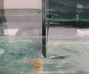
A series of experiments was carried out in the wave flume of the , in Le Havre, France. The LOMC wave flume is 35 m long, 1.2 m high and 0.9 m wide. It is equipped with a piston-type wavemaker at one end of the channel, and a sloping beach at the other end to reduce wave reflection. Two arrays of four resistive wave gages each are used for accurate free-surface elevation measurements. Throughout all experiments of this study, the water depth is 0.4 m. The general set-up is depicted in figure 5. Note that the wavemaker features an active wave absorption system, which efficiently prevents unwanted consecutive reflections on the wavemaker surface.

Figure 5. Wave channel set-up.
As depicted in figure 5, a polymethyl methacrylate plate is positioned vertically, centred across the channel width, approximately half-way between the wavemaker and the beach. The plate is hinged to the flume bottom, while it is maintained vertically by a force transducer, rigidly connected to the flume superstructure. Thus, the transducer force measurements give access to the total moment, about the hinge axis, of the fluid forces exerted by the flow on the barrier.
The resistive wave gages record the wave elevation with a 100 Hz sampling frequency, while the transducer has a 1000 Hz sampling frequency. In the latter case, the large sampling frequency allows for effectively filtering out the sensor noise, as detailed in Appendix B.3. In any case, most of the analysis presented in this work relies on the Fourier amplitude of the signals at the wavemaker frequency (between 0.4 and 1.2 Hz), which makes the sampling rates more than sufficient for the purpose of this study.
5.2. Experimental plan
Plates of three different width values,  $w = 20$, 40 and 60 cm, are studied. In each experiment, the wavemaker generates a monochromatic wave, with a target frequency and amplitude (as measured at the wavemaker position). The nominal frequencies range from 0.4 to 1.2 Hz, while the nominal amplitudes range from 2 to 80 mm. However, some frequency–amplitude combinations were not explored, to prevent possible damage onto the plate or transducer. In addition, in some of the experiments, large higher-order wave harmonics do not allow for accurate measurements of the energy budget. Those experiments were discarded, following the procedure outlined in Appendix B.3. Finally, the range of nominal frequencies and amplitudes, initially considered, and eventually included in the analysis, are summarised in the tables of figure 19.
5.3. Signal processing
Each experiment is at least 100 s long, to ensure that the steady state is reached along the whole channel length. The recorded signals are the eight resistive wave probe signals and the force transducer signal. For every experiment, only the second half of the record is used, to ensure that the steady-state regime is reached. The Fourier transform of each signal is calculated, at the prescribed wavemaker frequency. Prior to the Fourier transform, however, the signal is truncated so that its duration is a multiple of the prescribed wavemaker period, which mitigates frequency leakage. An example of experimental record is presented in more detail in Appendix B.3.
Eventually, each experiment results in 8 complex wave amplitudes  $\hat {\eta }_i$, $i = 1\ldots 8$, and the complex transducer force amplitude $\hat {F}_m$. The transducer force amplitude is used to infer the total excitation force in the pitch mode of motion, as explained in § 5.4, and the wave amplitudes are used to calculate forward- and backward-propagating wave components, in the up-wave and down-wave zones, using the procedure outlined in Appendix B.1, ensuring that the longitudinal dissipation in the flume is accounted for. Those wave components are employed to calculate the reflection and transmission coefficients, as also detailed in B.1.
5.4. Force measurements
The transducer force measurement  $F_m$ is related to the pressure forces as follows:
 \begin{equation} H F_m(t) = \int_{y= -w/2}^{w/2}\int_{z=0}^{h} z [p_-(y,z,t)-p_+(y,z,t)] \, \mathrm{d} z\, \mathrm{d}y, \end{equation}
where  $H = 0.80$ m is the height of the transducer with respect to the hinge axis, $h$ is the water depth and $p_-(y,z,t)$ and $p_+(y,z,t)$ are the pressure profiles onto the back and front sides of the barrier. Taking the Fourier transform of (5.1) in steady state, one recognises the generalised excitation force of (3.3), with the deflection mode $\zeta (z) = z$, which corresponds to a small pitch angle rotation about the plate hinge axis. Thus, the transducer measurements $\hat {F}_m$ and the hydrodynamic force $\hat {f}_{h}$ are related as follows:
 \begin{equation} \hat{f}_{h} = H \hat{F}_m. \end{equation}
 Thus, in our experiments, the generalised hydrodynamic force  $\hat {f}_{h}$ takes the form of the moment, about the barrier hinge axis, of hydrodynamic pressure forces.
5.5. Reflection and transmission coefficient measurements
The main focus of this work is to assess the effect of drag-induced dissipation on the far-field diffracted flow, which is described by means of reflected and transmitted travelling waves. With that aim, incident waves of various amplitudes and frequencies are sent to interact with the vertical plate, and the resulting transmitted and reflected waves are measured. As the incident wave amplitude is increased linearly, the magnitude of drag-induced forces should increase quadratically, so that the dissipated energy should increase cubically, while the incident wave energy increases with the square of the amplitude. The effect of drag on the far-field flow should then become more visible as the wave amplitude increases: with small wave amplitudes, very little departure from linear theory should be observed, while, with larger amplitudes, dissipation should have an appreciable effect on the flow, by withdrawing a significant fraction of the energy diffracted away from the structure.
More specifically, reflection and transmission coefficients should be affected, in a way which accounts for the energy withdrawn from the wave field, as discussed in § 3.1. By measuring transmitted and reflected waves propagating away from the structure, the ratio of energy dissipation is calculated as  $P_{d}/P_{wave} = 1-|\hat {R}|^2 - |\hat {T}|^2$, where $\hat {T}$ and $\hat {R}$ are the measured (complex) transmission and reflection coefficients. In addition, it can be assessed whether the dissipated energy is rather withdrawn from the transmitted wave, the reflected wave or both.
In summary, reflection and transmission measurements are instrumental in understanding the flow energy budget, and its drag-induced modifications. In addition, as shown in § 3.2, the reflection coefficient can also be used to estimate the excitation and drag force magnitude, as will be seen in § 6.2. The detail of the calculation of  $\hat {R}$ and $\hat {T}$, based on wave amplitudes $\hat {\eta }_i$, $i = 1\ldots 8$, is presented in Appendix B.1.
6. Results
6.1. Transmission and reflection coefficients
Reflection and transmission results are presented in figure 6 for the three plates, and for various frequencies and nominal wavemaker amplitudes, using the geometrical framework summarised in § 3. For each experimental point, its model counterpart (from the model of §§ 2.1 and 2.2) is plotted using the same marker shape and face colour, but with a black border. The dissipation-free model results (which do not depend on the wave amplitude) are also shown for each frequency, as black markers, which all rightly appear along the circle since no energy is dissipated.

Figure 6. Transmission coefficient in the complex plane: experiments and model. Black markers indicate the model dissipation-free coefficients. (a) Small plate –  $w=20\ {\rm cm}$. (b) Medium plate – $w=40\ {\rm cm}$. (c) Large plate – $w=60\ {\rm cm}$.
Let us first briefly comment on the linear behaviour of the barrier, i.e. the transmission coefficient for the smallest wave amplitudes. As frequency increases, transmission decreases (and reflection increases). Besides, at any given frequency, the transmission coefficient decreases with the plate width. In short, reflection is more important when  $kw$ increases. The precise location of $\hat {T}$, for the smallest incident wave amplitudes (where the least dissipation is expected to take place), is in reasonably good agreement with that predicted by the potential flow model of § 2.1 with no dissipation, and which is exactly located on the circle.
However, by examining figure 6(c), which shows reflection and transmission results for the largest plate, it can be noted that the potential flow model does not accurately capture the angular position of the transmission coefficient along the circle observed experimentally. This error, however, does not seem to depend on the incident wave amplitude, and thus cannot be attributed to an inherently nonlinear modelling error. A couple of tests, based on the numerical model of § 2, have helped us formulate plausible explanations. In practice, the plates were not perfectly rigid, so that appreciable deflection occurred during the experiments, of the order of 1 cm of maximum deflection for a 4 cm amplitude wave (8 cm trough to crest). Although relatively modest at first glance, for the largest plate the waves radiated by this motion may not be negligible, and thus may explain inaccuracies in the numerical results, which only represent the diffraction problem. Another possible explanation lies in the narrow width (15 cm) of the gaps between the large barrier edges and the flume vertical sidewalls. For the modelling of an oscillatory flow through narrow slots, it is customary to introduce a linear added inertial term in the boundary condition, with an empirically tuned ‘effective orifice length’ parameter, see e.g. Bennett et al. (Reference Bennett, McIver and Smallman1992) or Mei et al. (Reference Mei, Stiassnie and Yue2005), chapter 6. As pointed out in Appendix A.1, the addition of such an inertial term in our model is possible, although beyond the scope of this work. Since this added inertia is a linear, non-dissipative effect, it would result in a change in the angular position of  $\hat {T}$ along the circle contour. Nevertheless, in the absence of accurate plate deflection measurements throughout our set of experiments, we will not speculate further about the cause of the observed mismatch.
Now considering the effect of wave amplitude on the reflection and transmission coefficients, the experimental observations confirm that, as the wave amplitude increases, more and more energy (relative to the incident wave energy) is withdrawn from the wave field, as can be seen from the transmission coefficient location entering further inside the circle. The direction in which the transmission coefficient moves indicates that the dissipated energy is primarily at the expense of the transmitted wave, and yet does not, in general, leave reflection unchanged. In fact, the reflection coefficient may at times increase (for smaller  $kw$ values, i.e. small plate or small frequencies), or decrease (larger $kw$). The drag-induced far-field modifications are thus not as simple as either case 1 or 2 in figure 3, but, by comparing model and experimental points in figure 6, those modifications are relatively well captured by the pressure drop model of § 2.2.
Finally, a Morison force model would be consistent with a horizontal modification of the reflection coefficient, as discussed at the end of § 4. From figure 6, this only appears to be the case, experimentally, for low  $kw$ (especially for the small plate), i.e. precisely in the conditions where the forces are drag dominated, see figure 1. In contrast, the pressure drop model captures the drag-induced far-field modifications across all conditions.
6.2. Drag forces and power dissipation
We now turn our attention to a more quantitative analysis of the results. In this section, we intend to examine how the experimental drag forces compare with the predictions of the pressure drop model of § 2.2, and those of the Morison force model of § 4. Ideally, one would use the transducer measurements, which give access to  $\hat {f}_h = \hat {f}_0 + \hat {f}_d$, see (5.1). One would measure $\hat {f}_h$ for the smallest incident waves, which would be an approximation for $\hat {f}_0$, while other measurements of $\hat {f}_h$ would provide $\hat {f}_d$ through the relation $\hat {f}_d = \hat {f}_h-\hat {f}_0$. However, comparing the angle of $\hat {f}_h$ across experiments would require force measurements to be precisely synchronised across experiments (with respect to incoming waves).
Unfortunately, the wavemaker and wave probe measurement systems were distinct from the transducer data acquisition set-up, so that wave elevation and force measurements could not be precisely synchronised. This means that we do not have direct access to the phase relation between  $\eta$ and the hydrodynamic forces, and we thus cannot compare $\hat {f}_h$ across two different experiments.
However, we can make good use of (3.5) to infer the excitation force coefficient  $\hat {e}$ in each experiment, using solely the reflection coefficient measured and plotted in § 6.1. Before doing so, we verify experimentally the validity of (3.5), by comparing the magnitude of $\hat {f}_h$ (directly measured from the transducer) with that estimated through (3.5), as shown in figure 7. The agreement is found excellent for almost all experimental points. Therefore, it seems a valid approach to relate the hydrodynamic forces to the reflection coefficient, following (3.5).

Figure 7. Experimental measurement of hydrodynamic moment (excitation  $+$ drag): direct measurement through the force transducer vs indirect measurement through the wave reflection coefficient. (a) Small plate – $w=20\ {\rm cm}$. (b) Medium plate – $w=40\ {\rm cm}$. (c) Large plate – $w=60\ {\rm cm}$.
Denoting as  $\hat {R}_d = \hat {R} - \hat {R}_0$ as the difference in reflection coefficient between the drag-free and dissipative cases, the drag force can now be inferred as
 \begin{equation} \hat{f}_{d,est} = 2 g \rho W \gamma_0 \hat{\eta}_I \hat{R}_d. \end{equation}
It remains to estimate an experimental value for  $\hat {R}_0$. To do so, for each frequency and for each plate, the value $\hat {T}$ for the smallest incident wave amplitude ( $A_0 = 2$ mm) is projected onto the circle where dissipation-free coefficients should be located, thus yielding an estimate for $\hat {T}_0$ and $\hat {R}_0 = 1-\hat {T}_0$, as illustrated in figure 8 for the medium-size plate.

Figure 8. Experimental estimation of the drag-free transmission coefficient, for the medium plate ( $w = 40$ cm).
The drag moment magnitude, empirically estimated through the above procedure, is shown in figure 9, and compared with its model counterparts, obtained through the Morison force model (left-hand side figures) and through the pressure drop model (right-hand side figures). Both models seem to capture experimental results reasonably well. The surfaces show how the two models extend beyond the experimental range of amplitudes. Overall, the two models predict a similar drag force magnitude, except for larger  $kw$ values, where the curves of the pressure drop model bend significantly. This bending of the pressure drop model occurs for $kw \approx {\rm \pi}$, i.e. when the structure width is comparable to half a wavelength, and it can be interpreted as the diffracted flow having a substantial effect on drag creation.

Figure 9. Moment of drag forces. Each experimental point is vertically connected to its model equivalent through a dashed grey line. The surface represents how the model drag force extends across and beyond the experimental range. All model points (black squares) are located on the surface. (a,b) Small plate –  $w=20\ {\rm cm}$. (c,d) Medium plate – $w=40\ {\rm cm}$. (e, f) Large plate – $w=60\ {\rm cm}$.
Finally, the amount of dissipated power, relative to that of the incident wave, can also be measured as  $P_{d}/P_{wave} = 1-|\hat {T}|^2-|\hat {R}|^2$. Figure 10, which is organised identically to figure 9, compares this amount with its model equivalents, i.e. by integrating (4.6) over $z$ in the Morison force model, and by calculating $1-|\hat {T}|^2-|\hat {R}|^2$ in the pressure drop model (which is equivalent to, and easier than, using (2.10)).

Figure 10. Average dissipated power relative to incident wave power. Each experimental point is vertically connected to its model equivalent through a dashed grey line. The surface represents how the model dissipation extends across and beyond the experimental range. All model points (black squares) are located on the surface. (a,b) Small plate –  $w=20\ {\rm cm}$. (c,d) Medium plate – $w=40\ {\rm cm}$. (e, f) Large plate – $w=60\ {\rm cm}$.
The two models seem to perform similarly well under most conditions. However, the pressure drop model has a tendency to overestimate power dissipation for the small plate, more markedly so than the Morison force model. For the large plate, and for the larger  $kw$ values (which correspond to $f = 1$ Hz and $f = 1.2$ Hz), the Morison force model strongly overestimates the dissipated power. In contrast, the curvature of the pressure drop model accurately captures the experimental data, thus highlighting the importance of including the diffraction effect in the calculation of drag in cases where diffraction is dominant.
7. Conclusion
The experimental results clearly demonstrate the interplay between diffraction and drag-induced forces and dissipation. In all conditions, i.e. for drag- or diffraction-dominated flows, energy dissipation in the vortices has a marked effect on the far-field diffracted flow. Overall, the dissipated energy is subtracted predominantly from the transmitted wave, which is consistent with the results of previous studies (Stiassnie et al. Reference Stiassnie, Naheer and Boguslavsky1984) discussed in the introduction, but it would not be accurate to state that the reflected wave remains unchanged. In fact, depending on the frequency and magnitude of the incident wave, the presence of drag may reduce or increase the reflected wave amplitude with respect to that of a hypothetical dissipation-free scenario; additionally, in all cases, the phase of the reflection coefficient is modified.
Conversely, the results for the largest  $kw$ values (which correspond to the largest plate and largest frequencies) show that the diffraction-induced flow modification should be taken into account when calculating drag forces and dissipation. Indeed, in those cases, the experimental results show a marked bend, which is well captured by the pressure drop model (where the diffracted flow is represented), but not by the Morison force model (which is solely based on the incident flow).
Except for the latter case, the Morison force model compares well with experimental data, in terms of drag force magnitude and power dissipation. However, it does not account for the drag-induced far-field modification, nor does it represent accurately the phase of the radiation force, except for the drag-dominated flows (smallest  $kw$ values, which occur for the small plate).
The results from the pressure drop model, in terms of wave reflection and transmission, drag forces and dissipation, albeit imperfect, are satisfactory across all conditions. In particular, the far-field flow modification in the presence of drag seems to be realistically represented. Note that those results were obtained using a relatively crude pressure drop model, with only one parameter (namely, a dimensionless quadratic loss coefficient), which was kept identical throughout all conditions. The agreement with experimental points could certainly be improved, by fine tuning this parameter depending on the frequency and on the plate size. Introducing a second parameter governing, for example, the lateral extent of the virtual porous screen, would further enhance the results. However, instead of heading towards more complexity, the point of this work is rather to account for the diffraction–drag interplay with the least possible parameter tuning.
Funding
This project has received funding from the European Union's Horizon 2020 research and innovation programme under the Marie Skłodowska-Curie grant agreement no. 842967.
Declaration of interests
The authors report no conflict of interest.
Appendix A. Numerical solution methods
A.1. Scattering problem formulation
Consider the hydrodynamic problem described in § 2. The variables are all written as harmonic functions, as specified in (2.7). Thus, (2.2)–(2.6) can be reformulated in terms of the complex potential function. In the fluid domain, the Laplace equation reads
 \begin{equation} \nabla^2\hat{\phi} = 0. \end{equation}
At the free surface, the kinematic-dynamic boundary condition becomes
 \begin{equation} -\omega^2 \hat{\phi} + g \frac{\partial \hat{\phi}}{\partial z} = 0. \end{equation}
The no-flow conditions through the flume bottom and lateral walls are expressed as
 \begin{equation} \frac{\partial \hat{\phi}}{\partial z} = 0, \quad z = 0, \end{equation}
and
 \begin{equation} \frac{\partial \hat{\phi}}{\partial y} = 0, \quad y ={\pm} W/2. \end{equation}
 Finally, conditions apply over the vertical plane  $x = 0$, where the barrier is located. On the barrier, a no-flow condition applies
 \begin{equation} \frac{\partial \hat{\phi}}{\partial x} = 0, \quad x = 0, \quad |y| \leq w/2. \end{equation}
Without modelling the dissipation, the potential is continuous through the interface on the two sides of the barrier, that is
 \begin{equation} \hat{\phi}_+ - \hat{\phi}_- = 0, \quad x = 0, \quad |y| \geq w/2{,} \end{equation}
while the introduction of dissipation across a virtual porous wall, as in (2.9), takes the following form:
 \begin{equation} \hat{\phi}_+ - \hat{\phi}_- = \frac{jg}{\omega^2} \epsilon_l \frac{\partial \hat{\phi}}{\partial x}, \quad x = 0, \quad |y| \geq w/2. \end{equation}
We remark that conditions (A5), (A6) and (A7) generalise into the following condition, valid along the whole lateral extent of the flume:
 \begin{equation} \lambda(y) \left[ \hat{\phi}_+ - \hat{\phi}_- \right] = \frac{{\rm i} g}{\omega^2}\left[1-\lambda(y)\right]\frac{\partial \hat{\phi}}{\partial x}, \quad x = 0, \quad |y| \leq \frac{W}{2}, \end{equation}
where  $\lambda (y)$ is a real or complex function of $y$, which may vary continuously or stepwise, over the flume width.
First, considering that  $\lambda$ is a real-valued function, $\lambda (y) = 0$ amounts to condition (A5) (impermeable barrier condition), $\lambda (y) = 1$ amounts to condition (A6) (continuity condition) and $0 < \lambda (y) < 1$ amounts to condition (A7) (porous-wall condition), with the equivalence
 \begin{equation} \lambda(y) = \frac{1}{1+\epsilon_l}. \end{equation}
Eventually, the set of equations to solve reduces to (A1)–(A4), together with (A8).
The function  $\lambda (y)$, which we choose to call the ‘matching profile’, accommodates any $y$-wise variation in porosity. For example, it would be possible to make the profile vary continuously between $0$ at the barrier and $1$ far from the barrier, for a refined representation of where dissipation occurs the most. In addition, it would not be difficult to also make $\lambda$ vary with depth. Finally, in the study of porous screens and slotted or pierced barriers, it is not uncommon to find matching conditions also involving inertial terms, in the form
 \begin{equation} \hat{\phi}_+ - \hat{\phi}_- = \left[\frac{jg}{\omega^2} \epsilon_l + L \right] \frac{\partial \hat{\phi}}{\partial x}, \quad x = 0, \end{equation}
where  $L$ is an ‘effective orifice length’ parameter, see e.g. Bennett et al. (Reference Bennett, McIver and Smallman1992). In such a case, (A8) still holds, with $\lambda$ taking complex values
 \begin{equation} \lambda(y) = \frac{1}{1+\epsilon_l - {\rm i}\dfrac{\omega^2}{g}L}. \end{equation}
A.2. Matched eigenfunction expansion solution
We now turn our attention to the mathematical and numerical solution of (A1)–(A4) and (A8), through a matched eigenfunction expansion method. Although the approach relies on the same principle as that of Dalrymple & Martin (Reference Dalrymple and Martin1990) and Wang et al. (Reference Wang, Qiu, Ye and Liang2016), the more general matching profile formulations, proposed here, make it useful to provide the mathematical and numerical procedure in some detail.
Since the depth is constant, using separation of variables, the problem is decomposed into vertical fluid eigenmodes  $Z_n(z)$, $n \in \boldsymbol {N}$, see for example chapter 8 of Mei et al. (Reference Mei, Stiassnie and Yue2005). However, in the present diffraction problem, because the structure walls are perfectly vertical, only the flow component following the mode $Z_0$ is non-zero (Dalrymple & Martin Reference Dalrymple and Martin1990), where
 \begin{equation} Z_0(z) = \frac{\cosh k z}{\cosh kh}. \end{equation}
Hence, the scattered potential can be written as follows:
 \begin{equation} \hat{\phi}(x,y,z) = Z_0(z)(\hat{a}_I {\rm e}^{{\rm i}kx} + \hat{\varphi}_0(x,y)). \end{equation}
 In (A13), the first term  $\hat {a}_I Z_0(z){\rm e}^{{\rm i}kx}$ represents the incident potential flow, where $\hat {a}_I$ relates to the incident free-surface elevation amplitude $\hat {\eta }_I$ as follows:
 \begin{equation} \hat{a}_I = \frac{-{\rm i}g}{\omega} \hat{\eta}_I. \end{equation}
When solving the problem numerically, the incident potential amplitude is assumed equal to unity, i.e.  $\hat {a}_I = 1$.
The function  $\hat {\varphi }_0$ satisfies the Helmholtz equation
 \begin{equation} \left[\nabla^2+\kappa_0^2\right]\hat{\varphi}_0 = 0. \end{equation}
 Let  $\hat {\varphi }_0^-$ denote the solution in the up-wave zone ( $x\leq 0$), and $\hat {\varphi }_0^+$ the solution in the down-wave zone ( $x\geq 0$). Using again separation of variables, the $y$ dependency of the potential functions $\hat {\varphi }_0^-$ and $\hat {\varphi }_0^+$ is decomposed into a set of sinusoids. Also using the Helmholtz equation (A15) and the fact that the diffracted potential is always going away from the structure, one finds
 \begin{equation} \begin{cases} \hat{\varphi}^ -_0(x,y) = \displaystyle\sum\limits_{p= -\infty}^{\infty} \hat{a}^-_p \exp({{\rm i}(-\beta_p x + \alpha_p y)}) \\[10pt] \hat{\varphi}^+_0(x,y) = - \displaystyle\sum\limits_{p= -\infty}^{\infty} \hat{a}^+_p \exp({{\rm i}(\beta_p x + \alpha_p y)}), \end{cases} \end{equation}
where
 \begin{equation} \begin{cases} \alpha_p = \dfrac{2 p{\rm \pi}}{W}\\[10pt] \beta_p^2 + \alpha_p^2= \kappa_0^2, \end{cases} \end{equation}
and  $\hat {a}^+_p$ and $\hat {a}^-_p$, $p = -\infty \dots \infty$ represent two sets of unknown complex coefficients.
The modes of (A16) represent propagating waves for all  $|p|$ such that $\kappa _0^2-\alpha _p^2>0$, while larger values of $|p|$ yield evanescent modes, with amplitude decaying exponentially away from the structure location. Note that, in the case of an incident wave length $2{\rm \pi} /k$ larger than the channel width $W$, the only propagating mode is for $p = 0$.
In  $x=0$, the $x$-wise flow velocity is continuous through the interface between the up-wave and down-wave regions, that is
 \begin{equation} \frac{\partial \hat{\varphi}_0^+}{\partial x} - \frac{\partial \hat{\varphi}_0^-}{\partial x} = 0, \quad x = 0,\quad |y| \leq W/2. \end{equation}
Replacing  $\hat {\varphi }$ with its expression (A16), multiplying the equality by ${\rm e}^{-{\rm i}\alpha _n y}$, integrating over $y \in [-W/2;W/2]$ and using orthogonality of the functions ${\rm e}^{{\rm i}\alpha _p y}$, it is easy to find that $\forall p$, $\hat {a}^+_p = \hat {a}^-_p$, which allows us to drop the $\pm$ superscript and denote the unknown coefficients as $\hat {a}_p$ (see also Dalrymple & Martin Reference Dalrymple and Martin1990).
Finally, in order to determine the unknown coefficients  $\hat {a}_p$, (A16) is injected in the generalised matching condition of (A8), to derive the following equation:
 \begin{equation} G(y)=0, \quad |y| \leq W/2, \end{equation}
where
 \begin{equation} G(y) = \sum_{p= -\infty}^{\infty}\left[ \left(2-\frac{g\beta_p}{\omega^2} \right) \lambda(y) + \frac{g \beta_p}{\omega^2} \right] \hat{a}_p {\rm e}^{{\rm i}\alpha_p y} - \left[ 1-\lambda(y)\right] \frac{gk}{\omega^2}, \end{equation}
and
 \begin{equation} \lambda(y) = \begin{cases} 0 & (|y| \leq w/2), \\ 1 & (|y| > w/2). \end{cases} \end{equation}
 Equation (A19) can be solved using a spectral method, that is, by projecting the equation onto the basis functions  ${\rm e}^{{\rm i}\alpha _p y}$, up to a chosen truncation order. However, such a method was found prone to numerical inaccuracies. Therefore, instead, the equation is solved through the minimisation of the $L_2$ norm, i.e. by minimising
 \begin{equation} F(\hat{a}_{ -P},\ldots, \hat{a}_0,\ldots\hat{a}_P) = \int_{ -W/2}^{W/2} |G_P(y)|^2 \, \mathrm{d}y \end{equation}
with respect to the coefficients  $\hat {a}_p$, where $P$ is the truncation order, and $G_P$ is the $P$th-order truncation of $G$. The approach is thus similar to the one of Dalrymple & Martin (Reference Dalrymple and Martin1990), with differences in the implementation because of the different formulation for the matching function $G(y)$.
By writing the optimality condition
 \begin{equation} \frac{\partial F}{\partial \hat{a}_q} = 0, \end{equation}
for  $q = -P\ldots P$, one finds, after some cumbersome but simple algebra, the following set of $2P+1$ linear equations:
 \begin{align}
&\sum_{p= -P}^{P}\left[4 A_{p-q} +
\frac{g^2}{\omega^4}\beta_p \beta_q^* B_{p-q} +
\frac{2g}{\omega^2} \beta_p C_{p-q} + \frac{2g}{\omega^2}
\beta^*_q C^*_{q-p}\right] \hat{a}_p\nonumber\\
&\quad = \left[ \frac{k
g^2}{\omega^4} \beta^*_q B_{ -q} + \frac{2 k g}{\omega^2}
C_{ -q} \right],
\end{align}
\begin{align}
&\sum_{p= -P}^{P}\left[4 A_{p-q} +
\frac{g^2}{\omega^4}\beta_p \beta_q^* B_{p-q} +
\frac{2g}{\omega^2} \beta_p C_{p-q} + \frac{2g}{\omega^2}
\beta^*_q C^*_{q-p}\right] \hat{a}_p\nonumber\\
&\quad = \left[ \frac{k
g^2}{\omega^4} \beta^*_q B_{ -q} + \frac{2 k g}{\omega^2}
C_{ -q} \right],
\end{align}
where the terms  $A_p$, $B_p$ and $C_p$, $-2P\leq p \leq 2P$, are defined as
 \begin{equation} \begin{cases} A_p = \dfrac{1}{W} \displaystyle\int_{ -W/2}^{W/2} |\lambda(y)|^2 {\rm e}^{{\rm i}\alpha_p y}\, \mathrm{d}y \\[10pt] B_p = \dfrac{1}{W} \displaystyle\int_{ -W/2}^{W/2} |1-\lambda(y)|^2 {\rm e}^{{\rm i}\alpha_p y}\, \mathrm{d}y \\[10pt] C_p = \dfrac{1}{W} \displaystyle\int_{ -W/2}^{W/2} \lambda^*(y)\left[1-\lambda(y)\right] {\rm e}^{{\rm i}\alpha_p y}\, \mathrm{d}y. \end{cases} \end{equation}
 Once the  $2P+1 \times 2P+1$ linear problem of (A23) is solved, the excitation force can be found by integrating the pressure difference $\hat {p}_+-\hat {p}_-$ over the surface $x=0$, $|y|< W/2$, $0\leq z \leq h$. Because the deflection profile $\zeta (z)$ depends on $z$ only, the contribution of modes ${\rm e}^{{\rm i}\alpha _n y}$, $|n| \geq 1$, is zero, which yields
 \begin{equation} \hat{f}_h = 2{\rm i}\omega \rho W \gamma_0 \hat{a}_0, \end{equation}
where  $\gamma _0$ is the projection of the deflection mode onto the first vertical eigenmode, defined as follows:
 \begin{equation} \gamma_0 = \int_0^h \zeta(z) Z_0(z) \, \mathrm{d} z. \end{equation}
The reflection and transmission coefficients are simply given as follows:
 \begin{equation} \begin{cases} \hat{R} = \hat{a}_0, \\ \hat{T} = 1-\hat{a}_0. \end{cases} \end{equation}
Using (A14), the hydrodynamic force (A26) can be reformulated as
 \begin{equation} \hat{f}_h = \hat{e} \hat{\eta}_I, \end{equation}
where the excitation coefficient reads
 \begin{equation} \hat{e} = 2\rho g W \gamma_0 \hat{a}_0, \end{equation}
A.3. Lorentz linearisation
It remains to introduce a quadratic loss function at the interface as in (2.8), instead of the linear one of (2.9). Given a quadratic loss coefficient  $\epsilon _q$ and incident wave amplitude $\hat {A}$, one seeks to find a linear loss coefficient $\epsilon _l$, such that the quadratic and linear average power values $P_q$ and $P_l$, of (2.10), are equal. One could proceed iteratively, i.e. start with an initial guess $\epsilon _l^{(0)}$, calculate $P_q(\epsilon _l^{(0)})$ and $P_l(\epsilon _l^{(0)})$ and adjust $\epsilon _l$ as $\epsilon _l^{(1)} = P_q(\epsilon _l^{(0)})/P_l(\epsilon _l^{(0)})$, and so on with $\epsilon _l^{(i+1)} = P_q(\epsilon _l^{(i)})/P_l(\epsilon _l^{(i)})$, until some convergence criterion is met.
However, in this work, we rather adopt a different method, which avoids resorting to an iterative procedure for every new wave amplitude. By defining
 \begin{equation} R(\epsilon_l) = \frac{\omega}{2g\epsilon_l}\frac{ \displaystyle\int_{0}^T\int_{0}^h \int_{ -W/2}^{W/2} |\boldsymbol{\nabla} \phi_{\epsilon_l}|^2 \left|\dfrac{\partial \phi_{\epsilon_l}}{\partial x}\right| \mathrm{d}y \, \mathrm{d} z \, \mathrm{d} t}{ \displaystyle\int_{0}^T\int_{0}^h \int_{ -W/2}^{W/2} \left|\dfrac{\partial \phi_{\epsilon_l}}{\partial x}\right|^2 \, \mathrm{d}y\, \mathrm{d} z\, \mathrm{d} t}, \end{equation}
the quadratic-to-linear power ratio can be expressed as
 \begin{equation} \frac{P_q(\epsilon_l)}{ P_l(\epsilon_l)} = R(\epsilon_l) \epsilon_q |\hat{A}|. \end{equation}
 Thus, the potential solution  $\phi _{\epsilon _l}$ is first calculated for a wide enough range of $\epsilon _l$ values, and $R(\epsilon _l)$ is saved. Subsequently, for any values of $\epsilon _q$ and $\hat {A}$, the equivalent linear coefficient $\epsilon _l$ is found by numerically solving $R(\epsilon _l) = (\epsilon _q |\hat {A}|)^{-1}$. Finally, the corresponding potential solution $\phi _{\epsilon _l}$, and the results of interest such as hydrodynamic forces and reflection–transmission coefficients are calculated. Note that, although $\epsilon _q$ could be more finely tuned, it is kept equal to 1 throughout the present study.
Appendix B. Experimental data processing
B.1. Reflection and transmission coefficient calculation
Measuring reflected and transmitted waves requires the separation of forward- and backward-propagating wave components, in the up-wave and down-wave regions of the flume, using probe measurements. The procedure adopted in this work is based on the method of Mansard & Funke (Reference Mansard and Funke1980), which is slightly modified to account for longitudinal wave dissipation along the flume.
Assume, as we do in the rest of this article, that the wave frequency is below the flume cutoff, which ensures that the wavelength  $2{\rm \pi} /k$ is larger than the flume width $W$. Also assume that the waves are small enough for Airy's wave theory to be a valid representation. Far enough from the barrier, the damping beach or the wavemaker, the free-surface elevation thus consists of forward- and backward-propagating plane waves, which allows for writing
 \begin{equation} \eta(x,t) = {\rm Re} \{\hat{\eta}_{\rightarrow} \exp({{\rm i}(k(\omega)x - \omega t)}) + \hat{\eta}_{\leftarrow} \exp({{\rm i}( -k(\omega)x - \omega t)})\}, \end{equation}
where  $x$ is the longitudinal position along the flume, $x=0$ is the barrier position, the dependency of the wave field on $y$ has been dropped and the wavenumber $k$ depends on $\omega$ through the dispersion relation. Equation (B1) implies that the amplitude of each wave remains unchanged as the wave travels. In reality, however, the waves undergo longitudinal dissipation, which can occur predominantly at the flume bottom and sidewalls, and near the water surface. Dissipation can be accounted for by modifying (B1) as follows:
 \begin{equation} \eta(x,t) = {\rm Re} \{\hat{\eta}_{\rightarrow} \exp({{\rm i}(\tilde{k}(\omega)x - \omega t)}) + \hat{\eta}_{\leftarrow} \exp({{\rm i}(-\tilde{k}(\omega)x - \omega t)})\}, \end{equation}
where  $\tilde {k}(\omega ) = k(\omega ) + {\rm i}\nu (\omega )$ and $\nu (\omega )$ is a real, positive dissipation coefficient. The dissipation coefficient $\nu (\omega )$ is calibrated experimentally for each frequency using a series of barrier-free tests, which are detailed in § B.2.
Figure 11 illustrates how an incident (forward-propagating) wave is superimposed with a reflected (backward-propagating) wave, to form the total wave field. Both forward- and backward-propagating components undergo longitudinal dissipation, as represented in (B2).

Figure 11. Forward- and backward-propagating wave components with longitudinal dissipation (first and second graphs, respectively), as well as their sum as per (B2) (third graph). Each graph represents the wave elevation at a different instant across a wave period  $T_w$, indicated by the line colour.
In each zone of the flume (up-wave and down-wave), the signal  $\eta$ is recorded by a rack of 4 wave probes located at positions $x_i, i = 1\ldots 4$. The probe positions can be deduced from the distances specified in figure 12, bearing in mind that the barrier location is taken as the origin $x = 0$. In every experiment, the signal $\eta$, in steady state, is Fourier transformed at the wavemaker frequency $\omega _0$, to obtain a set of four Fourier coefficients $\hat {\eta }_i$, which are related to forward- and backward-propagating wave components through (B2), as follows:
 \begin{equation} \hat{\eta}_i = \hat{\eta}_{\rightarrow} \exp({{\rm i}\tilde{k}(\omega)x_i}) + \hat{\eta}_{\leftarrow} \exp({-{\rm i}\tilde{k}(\omega)x_i}). \end{equation}
Figure 12. Dimensions and distances in the wave flume, expressed in cm.
The two unknowns  $\hat {\eta }_{\rightarrow }$ and $\hat {\eta }_{\leftarrow }$ are found from the four equations using complex linear least squares. Doing so in the up-wave ( $-$) and down-wave ( $+$) zones yields four complex amplitude coefficients $\hat {\eta }^-_{\rightarrow }$, $\hat {\eta }^-_{\leftarrow }$, $\hat {\eta }^+_{\rightarrow }$ and $\hat {\eta }^+_{\leftarrow }$. If it is assumed that the dissipation beach perfectly prevents wave reflection in the down-wave zone ( $\hat {\eta }^+_{\leftarrow }=0$), then the plate reflection and transmission coefficients could simply be expressed as the fractions $\hat {R} = \hat {\eta }^-_{\leftarrow }/\hat {\eta }^-_{\rightarrow }$ and $\hat {T} = \hat {\eta }^+_{\rightarrow }/\hat {\eta }^-_{\rightarrow }$. However, it is more robust to estimate $\hat {R}$ and $\hat {T}$ in a way which accounts for possible backward-propagating wave component in the down-wave zone.
In general, the four complex amplitude coefficients  $\hat {\eta }^-_{\rightarrow }$, $\hat {\eta }^-_{\leftarrow }$, $\hat {\eta }^+_{\rightarrow }$ and $\hat {\eta }^+_{\leftarrow }$ are related to $\hat {R}$ and $\hat {T}$ as follows:
 \begin{equation} \begin{cases} \hat{\eta}^-_{\leftarrow} = \hat{R} \hat{\eta}^-_{\rightarrow} + \hat{T} \hat{\eta}^-_{\leftarrow} \\ \hat{\eta}^+_{\rightarrow} = \hat{T} \hat{\eta}^-_{\rightarrow}+ \hat{R} \hat{\eta}^+_{\leftarrow}, \end{cases} \end{equation}
and therefore
 \begin{equation} \begin{pmatrix} \hat{R} \\ \hat{T} \end{pmatrix} = \begin{pmatrix} \hat{\eta}^-_{\rightarrow} & \hat{\eta}^-_{\leftarrow} \\ \hat{\eta}^+_{\leftarrow} & \hat{\eta}^-_{\rightarrow} \end{pmatrix}^{ -1} \begin{pmatrix} \hat{\eta}^-_{\leftarrow} \\ \hat{\eta}^+_{\rightarrow} \end{pmatrix}. \end{equation}
 However, as already documented by Mérigaud et al. (Reference Mérigaud, Thiria and Godoy-Diana2021), the phase of  $\hat {R}$ from (B5) is highly sensitive to the exact distances between the probes and the barrier, while that of $\hat {T}$ is highly sensitive to the exact value of the wavelength (which, in experiments, may slightly deviate from the theoretical dispersion relation, due to the presence of a mean surface current, for example). To represent the two coefficients in the complex plane, we thus rather use the fact that $\hat {R} + \hat {T} = 1$ (Mérigaud et al. Reference Mérigaud, Thiria and Godoy-Diana2021), to determine $\hat {R}$ and $\hat {T}$ based solely on the magnitude of (B5), which is a procedure almost insensitive to the probe location and wavelength. More specifically, the law of cosines is used for the triangle of side lengths $1$,
$1$,  $|\hat {R}|_{exp}$ and $|\hat {T}|_{exp}$, as illustrated in figure 13. This yields two possible locations for $\hat {T}$, together forming a complex-conjugate pair. However, the linear potential flow model of § 2 predicts that the transmission coefficient is located in the upper half of the circle, as seen in figure 6. Thus, in the notations of figure 13, it can reasonably be assumed that $\hat {T}_1$ should be chosen.

Figure 13. Geometrical determination of the phase of  $\hat {T}$, using the law of cosines.
B.2. Dissipation calibration
To calibrate the dissipation coefficients, experiments are carried out without the barrier. Similarly to the procedure described in § B.1, forward- and backward-propagating wave components are separated at the up-wave ( $-$) and down-wave ( $+$) probe racks, assuming $\nu = 0$ in (B2). Implicitly, such an approach assumes that the dissipation is negligible over the span of each probe rack. By doing so, one finds $\hat {\eta }^-_{\rightarrow }$ and $\hat {\eta }^+_{\rightarrow }$, with $|\hat {\eta }^+_{\rightarrow }| \leq |\hat {\eta }^-_{\rightarrow }|$, due to the longitudinal dissipation taking place over the distance between the two probe racks.
Defining as  $\bar {x}_-$ and $\bar {x}_+$ the average longitudinal positions of the up-wave and down-wave probe racks, respectively, the dissipation coefficient $\nu$ is found as
 \begin{equation} \nu = \frac{\log|\hat{\eta}^+_{\rightarrow}| -\log |\hat{\eta}^-_{\rightarrow}|}{\bar{x}_+ -\bar{x}_-}. \end{equation}
 For each frequency,  $\nu$ is estimated for three incoming wave amplitudes (2, 4 and 10 mm), to ensure that the coefficient does not exhibit a strong wave-amplitude dependency. The results are summarised in figure 14, which indeed suggests that the dissipation coefficient is relatively similar across wave amplitudes, while increasing consistently with the frequency. The average value (dashed line in figure 14) is retained, and used in (B3) to identify forward- and backward-propagating wave components, throughout all experiments.

Figure 14. Empirically estimated dissipation coefficient for different wave amplitudes and frequencies.
B.3. Data quality and selection
Figures 15, 16 and 17 show a detailed example of the recorded experimental signals, where the target wave amplitude is 8 mm and the wave frequency is 1.2 Hz. The 1.2 Hz frequency is chosen as an example because, among the frequency values of the experimental plan, 1.2 Hz waves are those with the slowest propagation speed, and it is therefore the frequency for which the steady-state regime takes the most time to be reached.

Figure 15. Wave probe signals from the up-wave probe group,  $f_0=1.2$ Hz, $A = 8$ mm.

Figure 16. Wave probe signals from the down-wave probe group,  $f_0=1.2$ Hz, $A = 8$ mm.

Figure 17. Force transducer signal,  $f_0=1.2$ Hz, $A = 8$ mm. The raw, unfiltered signal is shown by thin grey lines.
Figures 15 and 16 show the raw signals from the up-wave and down-wave resistive probe groups, respectively, together with the steady-state segment of the data extracted for Fourier analysis, as mentioned in § 5.3, corresponding to an integer number of wave periods.
Figure 17 shows the force transducer measurements for the same experiment (8 mm wave amplitude and 1.2 Hz wave frequency), also highlighting the transition to steady state. The transducer measurements are subject to significant measurement noise (in the present example, of magnitude comparable to the signal). However, the noise is essentially from the power supply, so that all the noise energy is located at the 50 Hz utility frequency and its higher harmonics. In this context, the 1000 Hz sampling rate of the transducer makes it easy to effectively suppress most of the noise using frequency-domain filtering, adopting 10 Hz as a cutoff frequency: the signal is Fourier transformed, the frequency components above 10 Hz are set to 0 and the signal is then transformed back to the time domain through the inverse Fourier transform. Figure 17 shows both unfiltered and filter signals.
The initial experimental plan included waves with amplitudes ranging from 2 to 80 mm, and frequencies between 0.4 and 1.2 Hz. However, the experiments for some pairs of conditions were eventually not carried out, when the plate deformation became too important, which may have led to damage to the plate itself or to the connection with the force transducer.
In some experiments, typically with the largest wave amplitudes, significant higher-order wave effects are visible, either by examining the time trace of the wave signal (figure 18a), or by analysing the frequency content of the waves (figure 18b). For low wave frequencies, the flume represents shallow water conditions, and as the wave amplitude grows, the wave signal takes an asymmetric shape resembling cnoidal waves (left-hand side of figure 18a). At larger wave frequencies, as the wave steepness increases, the wave crests become sharper and the wave profile approaches a higher-order Stokes wave (right-hand side of figure 18a). In addition to those nonlinear wave profiles, which result in bound harmonics, the possibly nonlinear wave–structure interaction at the barrier may result in the creation, and propagation, of free harmonics.

Figure 18. Nonlinear wave effects measured at the up-wave probe rack, in the experiments with the small plate ( $w = 20$ cm). (a) Phase-averaged wave pattern, measured by the first probe, at the lowest (left-hand side) and largest (right-hand side) frequencies. The bottom graphs show the same wave patterns, normalised by their $L_2$ norm, so that the changes in wave shape, with increasing wave amplitude, can be better appreciated. (b) Fourier amplitudes of the wave signal (averaged over the four up-wave probes), at the incident wave frequency $f_0$ and its harmonics, at the lowest (left-hand side) and largest (right-hand side) frequencies. In the bottom graphs, the same amplitudes are shown, normalised by that of the fundamental $f_0$.
Regardless of the causes for the observed higher-order harmonics, seen in figure 18(b), the energy budget established through the Fourier analysis at the incident wave frequency, as described in § B.1, is certainly biased when a significant fraction of the energy is diverted to those harmonics. In addition, in such cases, the linear summation of forward- and backward-propagating waves, which is the basis for the calculation of reflection and transmission coefficients, can no longer be assumed. Therefore, those experiments, where wave nonlinearities jeopardise the accuracy of experimental results, are discarded. As a nonlinearity measure, the amplitude ratio of the first harmonic to the fundamental, at the up-wave probes, is chosen, and the experiments where that ratio exceeds 15 % are discarded, i.e.
 \begin{equation} \left|\frac{\hat{\eta}(2f_0)}{\hat{\eta}(f_0)} \right| \geq 15\,\%. \end{equation}
In the examples shown in the bottom graphs of figure 18(b), one would discard those experiments where the second peak (at  $2f_0$) exceeds 0.15.
Figure 19 summarises the frequency–amplitude conditions which are eventually exploited in this article (blue entries), those for which the experiments were carried out but discarded based on the criterion of (B7) (red entries), and those which were not carried out (grey entries).

Figure 19. Frequency–amplitude conditions for the small (a), medium (b) and large (c) plates, which are eventually exploited in this article (blue entries), for which the experiments were carried out but discarded based on the criterion of (B7) (red entries), and which were not carried out to preserve the set-up integrity (grey entries).


 Open access