1. Introduction

In 1988/89 the Swedish Antarctic Research Programme (SWEDARP) built the research station Wasa on the Basen nunatak, Dronning Maud Land (DML) (73˚02' S, 13˚25' W). Since then glaciologists have been able to maintain a continuous scientific program in the Vestfjella–Heimefrontfjella area. One important question is whether this small drainage area in DML is in balance with present climate. Previous work in this area includes numerous studies of present and past snow-accumulation rates, ice and air temperatures, aerial cover of blue ice, ice surface elevation, bed topography and ice dynamics (Table 1).

Table 1 Relevant previous work

In this paper, we focus on Plogbreen (Fig. 1), one of two ice streams draining the Ritscherflya ice field (the other is the ∼20 times larger ice stream Veststraumen). Plogbreen covers approximately 20–25km in width and 60 km in length from the higher ground at Herculessletta to the grounding line at Riiser-Larsen Ice Shelf. The ice surface decreases from 750ma.s.l. at the ice divide on Herculessletta (near Ritscherflya) to about 150ma.s.l. at the grounding line 10– 15 km northwest of the Vestfjella mountain range. The most prominent features in this area are the nunataks Basen and Plogen, which constrain the ice flow through a channel-like section at about 200 –250 ma.s.l. (Fig. 1).

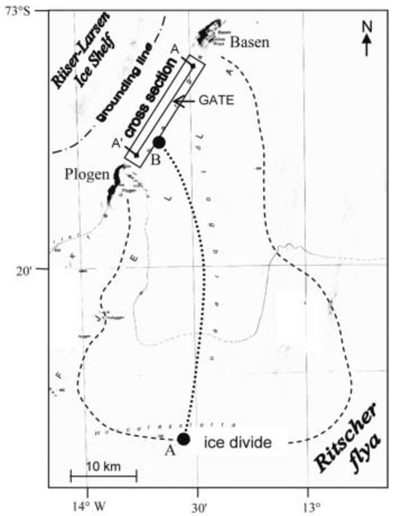
Fig. 1. Overview of the study area. The rectangle at the cross-section shows the approximate area/gate of the DGPS and GPR surveys. The dashed line is an outline of the catchment area. The dotted line represents the trajectory path used in the modeling of temperature with ice depth, where A and B stand for different stages in the model algorithm. Also included in the northwest corner is the approximate location of the grounding line. Swarms of small triangles indicate zones of observed crevasses.

Previous unpublished radar sounding measurements between Basen and Plogen indicate an overdeepening in the south reaching ice depths of 1000 m with the base below sea level (personal communication from J.-O. Reference Näslund and ReuterskiöldNäslund, 2003). Measured ice surface velocities reach a maximum of ∼100ma^–1 in the same area (Reference Holmlund, Richardson and OerterHolmlund and others, 1989). Crevasses in the area are mainly associated with the grounding line and restricted areas with relatively steep slope gradients. However, crevasses are also found in large flat areas completely lacking topographic undulations.

The accumulation rate varies from 0.25 mw.e. a^–1 on Ritscherflya to 0.40 mw.e. a^–1 on the Riiser-Larsen Ice Shelf, while average values for Plogbreen are 0.32–0.34mw.e. a^–1 (Reference HookeIsaksson and Karlén, 1994a).

Until recently, most studies have focused on Veststraumen. The physical setting of Plogbreen in combination with the available background data makes Plogbreen a suitable target for further studies of ice flux in relation to climate change. We aim to determine whether Plogbreen is in steady state by comparing ice influx, φ _in, with outflux, φ _out. φ _out is calculated at a gate (Fig. 1) using Glen’s flow law aided by a thermodynamic model and force-budget estimations from a model fed by measurements of ice surface velocities and ice geometry. φ _in is based on calculations of ice accumulation upstream of the gate. The input data are presented further below.

We first present the velocity and geometry data along with a brief description of collection techniques. The theroretical background for the numerical scheme used to calculate φ _out is well established and we do not describe it in detail; however, the major steps are shown in section 3. In sections 4–6 respectively, we present the results, followed by a sensitivity test and concluding discussion.

2. Data

A detailed study of the ice surface velocity and bed topography of Plogbreen, DML, Antarctica, was undertaken in the austral summer of 2002/03. Presented below are the data collection techniques and the data.

Repeated L1 carrier-phase differential global positioning system (DGPS) measurements of 40 evenly spaced aluminium stakes were used to construct a grid of ice surface velocities in a section where Plogbreen flows between two nunataks, Basen and Plogen (Fig. 1). The frame of the grid covered 3 km along and 18 km transverse to the ice-flow direction. The spatial extent was limited by crevassed areas both upstream and downstream of the chosen area. The maximum distance between the rover antenna and the reference station was 21 km. The first stake survey took place on 23–25 December 2002 followed by a second survey 3weeks later on 17–18 January 2003. The instrumentation (MK-1 receivers from DataGrid) was pre-tested to provide 0.01 m accuracy in the horizontal plane (x, y) and 0.25m accuracy in the vertical plane (z) using static recording mode for 15 min. This measurement technique was used consistently throughout both surveys, together with an accurately established fix point at the Swedish station Wasa (Reference Korth, Perlt, Dietrich and DietrichKorth and others, 2000) located on the Basen nunatak. During the recording epochs, the number of satellites was never allowed to fall below six during the post-processing procedure, generating an average uncertainty of ±1%. Considering the Antarctic severe ionospheric conditions in combination with single baseline measurements, the errors in achieved positions are probably larger than specified by the GPS manufacturer. By using only the relative movements of the stakes, we apply similar errors to all measurements when calculating velocity vectors. This way, the data prove consistent even for very short measurement intervals.

The ice surface slope was obtained directly from the vertical coordinate (z) in the DGPS survey of the 40 stakes. Ice depth was determined by a total of 174 km of ground-penetrating radar (GPR) transects using 8 MHz dipole antennas with a 20m antenna separation. A Tektronix THS 720 oscilloscope docked to a laptop permitted logging of 2500 samples per shot using a time window of 20 μs. The distance, d from transmitter to the ice–bedrock interface was calculated as:

(1)

where c is the speed of an electromagnetic wave in a vacuum, ε _ice is the dielectric permittivity of ice (here ε _ice = 3.2 assuming constant ice density; personal communication from J. Moore, 2002) and TWT is the two-way travel time of a radio wave (neglecting refraction effects). Each transect was surveyed twice and interpreted separately to ensure the bedrock location within an error range of ±10%.

The ice body is assigned a grid system with three dimensions, x, y and z, with a certain cell size. In this case, x and y directions will represent the horizontal plane, and the z direction represents the vertical plane counted positive downwards. The data and results are presented in a rotated local grid system (for efficient calculation) ranging from 0 to 3 km in the horizontal x direction (parallel to glacier flow direction), 0 to 18 km in the horizontal y direction (perpendicular to glacier flow direction) and 0 to 1200m in the vertical z plane (ice depth). The spatial resolution, i.e. grid interval, is set to 100 m, and the vertical depth integration step length is 1 m. The data are fitted to the grid system by using an interpolation technique described in Reference SandwellSandwell (1987). The force-balance model (described below) considers each point in the grid system; however, gradients are calculated using a spatial interval corresponding to average ice depth.

Ice surface velocities and elevation from the DGPS campaign are presented in Figure 2a–c, and the GPR-derived ice depth in Figure 2d. The results from the GPR campaign suggest there is a significant overdeepening down to 850 m below sea level in the southwestern region of the surveyed area, near the Plogen mountain range, after which the bedrock gradually rises to near sea level in the central and northeastern parts of the glacier. This corresponds to a maximum ice depth of ∼1100m near Plogen, ∼500m in the central parts, gradually decreasing to ∼200m near the Basen nunatak. The pattern of the horizontal surface velocities strongly reflects the bedrock topography by showing fast-flowing ice in the deep channel near the Plogen massif (y = 12–16 km). Lower velocities are observed from the trough towards the Basen nunatak, with the exception of a local maximum just east of the center line (y = 7 km) where the bedrock tends to deepen slightly. Both the velocity and geometry data correspond roughly with previous measurements in this area (personal communication from P. Reference HedforsHolmlund and J.-O. Näslund, 2003).

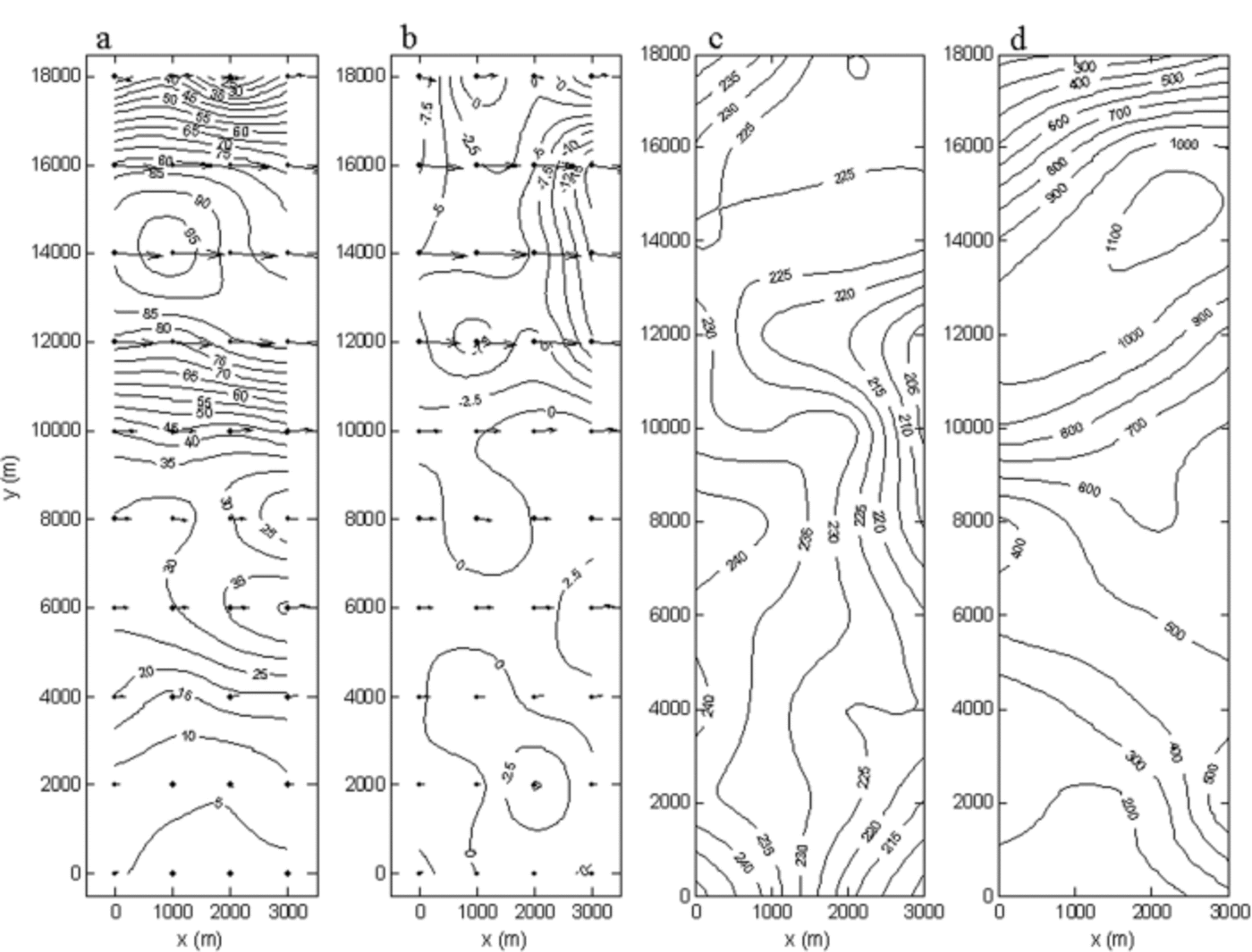
Fig. 2. Collected field data. (a, b) Horizontal surface velocities (m a^–1) in the x and y directions respectively. Arrows show relative velocity vectors projected from the actual 40 stake positions (black dots). (c) Surface elevation (m a.s.l.) (locally referenced). (d) Ice depth (m). The GPR recording traveled straight (twice) in between all stake columns (perpendicular to ice flow) and rows (parallel to ice flow). The figure uses a local coordinate system rotated approximately 160˚ in comparison with the frame outlined in Figure 1 (the top of the figure stands toward Plogen and the bottom is near Basen).

The drainage area of Plogbreen was outlined using satellite imagery in combination with Advanced Very High Resolution Radiometer (AVHRR)-based photoclinometry-derived digital elevation models (data from National Snow and Ice Data Center (NSIDC), Boulder, CO, USA), and estimated to 1420 ± 300km². This gives a total inflow of φ _in=0.48±0.1 km³ a^–1 from the upstream area, based on the accumulation rate, 0.33 ± 0.01mw.e. a^–1 (Reference IsakssonIsaksson and Karlén, 1994a). The error in accumulation rate (± 0.01mw.e. a^–1) was estimated from the variation in accumulation rates between two ice cores taken downstream and upstream of the major accumulation area (0.34 and 0.32 mw.e. a^–1 respectively).

3 Method

Irrespective of glacier shape, the flow through a cross-sectional gate, φ _out, should balance the incoming mass upstream, φ _in (Reference ClarkeClarke, 1987; Reference HookeHooke, 1998). Due to a temporal change in the mass balance, or in the ice-dynamical situation, this balance may deviate. φ _in is found by integrating the accumulation rate over a confined drainage basin (Fig. 1) upstream of the cross-section (presented above as data). φ _out is found through Glen’s flow law where deformation of ice (′′) is in constitutive relation to the temperature (T)-dependent viscosity (B) and shear stress (τ _e and τxz). Using x and z for longitudinal and vertical directions respectively, the relation is written:

(1)

where the experimental flow exponent n=3 and U is ice velocity. The value of B is calculated following Reference Pohjola and HedforsPohjola and Hedfors (2003), giving B=B ₀ exp(T ₀/T); B ₀ = 1.928 Pa a^(1/n) and T ₀ = 3155 K. The stress components, τ _e and τxz , depend on the force balance for the gate at the local site (Fig. 1 and 2). Once the strain rates with depth are known, φ _out is given by integrating velocity over cross-sectional length (y direction). φ _in is then compared with φ _out to test for steady-state conditions. Below are descriptions of the methodology in obtaining, first, the ice temperature needed for the viscosity calculations and, second, the force balance that provides information on the stress components.

3.1. Ice temperature

The viscosity is known to decrease as temperature increases, leading to increased deformation rates in accordance with Glen’s flow law (Reference PatersonPaterson, 1994). Hence, much of the deformation takes place in the bottom layers where temperature is raised due to geothermal heat, ice compaction and heat production from internal heat sources. The ice temperature depth profiles were modeled using a thermodynamic model described as:

(3)

where T is temperature, t is time, c is specific heat capacity, K is thermal conductivity, ρ is ice density, and Q is heat generated from internal and external heat sources (Reference Pohjola, Hedfors and HolmlundPohjola and Hedfors, 2003). The parameters c and K are functions of temperature, and their empirical relations are given in Reference PatersonPaterson (1994).

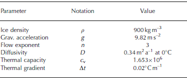
Model input to Equation 1 consists of ice surface temperatures, T _s =–18˚C (Reference Isaksson and KarlénIsaksson and Karlén, 1994b), an accumulation rate of 0.25mw.e. a^–1 (Reference Isaksson and KarlénIsaksson and Karlén, 1994a), an estimated average ice depth, H= 1000 m, and average surface slope, α=0.7˚. The vertical velocity, w, is assumed to decrease linearly with depth to a value of zero at the bed. The geothermal heat flux is set constant through the experiment. Additional constants used are presented in Table 2. For simplicity, the same temperature profile is used laterally towards the mountainsides at the site of the cross-section, where the vertical extension is compressed into the actual ice depth at the specific coordinate.

Table 2 Constants used for temperature modeling

The ice-temperature runs were divided into two different stages. The first stage calculates a steady-state profile over 10 000 years for the accumulation area adjacent to the ice divide (A in Fig. 1). Secondly, this profile is allowed to move 500 km downstream, from the ice divide to the site of the gate (B in Fig. 1), picking up heat over a period of 1000 years predominantly from internal heat production due to deformation. This produced the temperature profile used for the force-balance calculations shown in Figure 3.

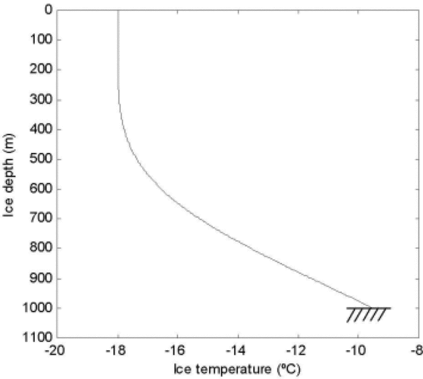
Fig. 3. Calculated ice temperature profiles using one stage of steady-state modeling followed by a stage of temperature development due to higher driving stresses.

3.2. Force balance

We have chosen to present only the fundamental laws of the force-balance method to find the stress conditions at the gate. Full numeric solution procedures are found in Reference Van der VeenVan der Veen and Whillans (1989), Reference Van der Veen and WhillansVan der Veen (1999), Reference HedforsHedfors (2002) and Reference Pohjola and HedforsPohjola and others (2004).

Taking resistive stresses constant with depth and neglecting vertical resistive stresses, we can write the so-called isothermal block-flow model for the horizontal direction, x as:

(4)

where the driving stress, τ _d x, is balanced by basal drag, τ _b x, and resistive stresses, Rxx and Rxy, for ice depth H (Reference Van der VeenVan der Veen and Whillans, 1989). The purpose is to solve for basal drag (τ _b x) which in turn provides the means for calculating the shear stress (τ _e and τxz) used in Equation 1. The driving stress in the longitudinal direction is calculated from the glacier geometry through the familiar expression:

(5)

where g is the gravitational acceleration (9.82 ms^–2) and ∂z/∂x is the surface slope. Measured surface velocities are used to determine the strain rates (έ _e, and έ _ij ; i, j = x, y, z) from which the resistive stresses at the surface are calculated via deviatoric stresses as:

(6)

and

(7)

using a value of B calculated from the average temperature in the bottom third of the modeled temperature profile (650– 1000 m in Fig. 3). The effective deviatoric stress (τ _e) is described analogous to effective strain rate as:

(8)

where

(9)

Since the calculated resistive stresses act on the body in all planes except at the base, the force budget must be balanced by a basal shear stress component, basal drag (τ _b x), which now can be calculated as the only unknown in Equation 1. Equation 1 is simplified assuming τ _e is constant with depth, which allows depth-integrated values from the force budget to be used. The vertical stress component, τ_xz , is set to zero at the glacier surface and increases linearly to a value equal to the basal drag at the bed.

3.3. Ice flux

Horizontal velocity with depth, U_x , is calculated at the cross-section using Equation 1 with the stress information obtained from the force-balance model above:

(10)

where m is the level below the glacier surface and w is found from the vertical velocity distribution calculated from the vertical strain rates (έ _zz ); w is assumed to be zero at the bed. The ice flux is determined by integrating the calculated horizontal velocity in the longitudinal direction (x plane) over the ice depth and length of the chosen cross-section in the transverse direction (y plane):

(11)

where h–b is total ice thickness and A–A' represents the length of the section in the horizontal y plane.

4. Results

A force-balance study generally produces a wide range of spatially and temporally distributed dynamical parameters such as strain rates, stress deviators and components of driving and frictional stresses which in themselves deserve a thorough discussion. Our results focus on the ice flux given from the distribution of the horizontal ice velocity with depth. In relation to this, horizontal distribution of basal drag and effective strain rates with depth are presented with the aim of understanding the dynamical situation in the vicinity of the cross-section on Plogbreen. Figure 4a–c show the resulting basal drag at the bed, the depth-integrated effective strain rates and the horizontal velocity component perpendicular to the cross-section, respectively, at the chosen cross-section defined by the coordinates, x = 1.5km and y = 1–17 km.

Fig. 4. (a) Horizontal projection of basal drag, τ _b x (kPa), with the cross-section marked (dashed line) at x = 1500m (A–A'). Ice flow is from top to bottom. (b) Depth-integrated effective strain rates, έe (a^–1). (c) Horizontal velocity with depth, Ux (ma^–1). The effective strain rate (b) and velocity field (c) are shown looking upstream with a depth exaggeration (×4) for better visualization.

Basal drags are highest in the deeper parts near Plogen, since this part has the highest driving stresses (mainly due to the large ice depth). The longitudinal decrease in basal drag at x = 1.2–1.6km and y = 14 km may be due to the fact that the grounding line appears just 10–15km downstream of the investigated area (Fig. 1). High drags (300 kPa) are observed at the northeastern margin at y = 1 km. These may be caused by increased pressures from the turning of flow around Basen in combination with low temperatures in the relatively shallow ice.

The effective strain rates, έ _e, shows values of up to 0.5 a^–1 near the bed in the deepest section. We also observe relatively high strain rates near the surface at y = 11 km, separating the flow in the deep channel from a parallel flow at y = 8 km. This is likely to indicate that the deeper channel is dynamically separated from the shallow area, and that the contact between the ice bodies is separated by a shear zone. An area of crevasses has been observed in the central parts of the glacier a short distance upstream of the cross-sectional area (Fig. 1). The origin of these crevasses is not fully understood, but the shear zone revealed by our calculations provides a logical explanation for their genesis.

The horizontal velocity in the x plane, U_x , indicates that the deep trough dominates the flux, but the width of the glacier makes the low velocities in the northeast region a significant contributor (∼12%) to the total ice flux.

The calculated outgoing volume gives φ _out=0.55km³ a^–1. At a first glance, this provides a negative balance for this glacial system if compared to the incoming ice flux, φ _in=0.48 km³ a^–1. Before any conclusions can be drawn, we need to consider the model sensitivity to errors in the incoming- and outgoing-flux components.

5. Sensitivity Tests

The methodology used does not allow a straightforward test of all parameters involved, but a few fundamental elements such as accumulation area, accumulation rates, the flow exponent, n, ice depth and surface velocities can be treated to vary within their error ranges.

The delineation of the ice divide was estimated to fall within a 5km accuracy. Since the exact drainage area is difficult to estimate, it also comes with the highest uncertainty (Reference Price and WhillansPrice and Whillans, 1998). Together with the error in accumulation rate, this generates an average error range of ±23% in the total incoming ice flux. For comparison, Reference Fricker, Warner and AllisonFricker and others (2000) found an uncertainty of ±20% in the incoming mass in their precipitation model as they compared measured and modeled balance fluxes for the Amery Ice Shelf, East Antarctica.

The outgoing ice flux has a lower average error range of ∼±10%, when adding up the effect of the different input parameters. The flow exponent was tested with values ranging from 2.5 to 3.5, where the most commonly used value for glacier ice is 3 (Reference PatersonPaterson, 1994). The effect of this variation on the calculated ice flux is small (±2.1%). The ice velocity has the lowest uncertainty due to good instrumentation accuracy and well-established surveying techniques (±1%). The error was estimated by applying maximum instrument error (0.02 m) to the average movement of the stakes (∼3m) between the recording occasions (25 days). Errors of ±3% (±1 dm of average movement) were tested to show a non-significant change in calculated outflux. The ice depth derived from the GPR survey was assigned a large error (±10%) due to the complexity of interpreting radio waves. The possibility of independently interpreting the same transect twice provided a good tool to estimate the error in the interpretation phase. This gave errors within ±5%, but additional errors reside in the mathematics. Refraction effects were neglected and a constant value for dielectric permittivity of ice was assumed. This has implications for the result; however, since our measurements fell within ±10% of values obtained on previous radar sounding campaigns, a ±10% error seem reasonable.

The force-balance model used is simple to implement but has drawbacks. The viscous terms in the balance calculation (the last two terms in Equation 1) tend to be overestimated if surface values are applied to the entire glacier thickness. Hence, the inferred value of basal drag is a limiting value. The other extreme is found by setting the basal drag equal to the driving stress (B = 0). The actual basal drag should fall between these two extremes and this is recognized in our force-balance calculations by applying the lower part of the modeled temperature profile to the isothermal block-flow scheme.

The contributions of each numerical error to the balance calculations are summarized in Table 3. Figure 5 shows the balance calculations of incoming (φ _in) and outgoing (φ _out) volume, with the combined maximum errors projected on each flux component. The result is a balanced system, within the error bars; φ _out = 0.55 ± 0.05km³ a^–1 and φ _in = 0.48 ± 0.1km³ a^–1. However, if the errors are not combined in the worst way, the trend points toward a system in a negative state – the mass leaving the system exceeds the incoming mass.

Fig. 5. Calculated incoming and outgoing ice flux with estimated errors.

Table 3 Tested error ranges (%)

6. Concluding Discussion

Establishing mass balances for Antarctic glacial systems involves the handling of large uncertainties. Especially when considering the incoming mass, large uncertainties arise from outlining the drainage area and from determining the temporally and spatially variable accumulation rate. A better way of finding the mass flux seems to be through ice-flow calculations in a well-confined area that represents the outgoing mass. In this paper, the uncertainty of the calculated outflux was less than half of that of the incoming mass. When put bluntly, our data show a balanced system, or even a positive balance, within the uncertainty limits. By only considering the median values of the flux components, the Plogbreen system can be said to be in a negative state where the mass leaving the system is greater than the incoming mass. This is also suggested from ice-core records showing a falling trend in accumulation (–25%) over the past 70 years (Reference IsakssonIsaksson and Karlén, 1994a). The transport time from precipitation to flow through the cross-section is roughly 1000 years if average surface velocities are assumed to be around 50ma^–1. Present-day measurements may reflect higher accumulation rates in the past, but, looking further back in time, no such trend in accumulation is available to support greater influxes centuries ago. More interesting is the glacier’s proximity (∼10 km) to the grounding line and the sub-sea-level overdeepened trough (∼800m below sea level) observed towards the Plogen massif. This environmental setting may allow for detection of signals of global warming. Thus, as a speculative comment, we argue that the indications of a negative mass balance can be explained by the recent rise in global sea level, as it is likely to induce glacier acceleration due to a reduction in resistive forces at the site of the gate. The argument is supported by observations of recent ice-shelf break-up at the Riiser-Larsen Ice Shelf in front of Plogbreen. However, more studies of a similar kind in this area are required to fully understand the processes that affect the glacier response to climate change. Accordingly:

• 1. We find that, within the uncertainty limits, the ice flux of Plogbreen is balanced between incoming and outgoing mass;

• 2. The result indicates a negative mass balance considering the median values of both components. This is to some extent supported by the trend in accumulation rates over the past 70 years, but may, speculatively, be an indication of glacier acceleration due to global warming and sea-level rise – an early warning signal of ice-shelf collapse in front of Plogbreen;

• 3. The calculated outgoing volume is a better estimate of the balance flux than the incoming volume, due to smaller uncertainties.