


1 Introduction
The design decisions that have the highest impact on the final design’s performance and cost are made during the early conceptual phase of the design process in which design criteria are not fully formulated and multiple design alternatives are explored (Krish Reference Krish2011; Østergård et al. Reference Østergård, Jensen and Maagaard2016). However, even though most computer-aided design (CAD) software provide capability to support the latter stages of design, with functionality such as fine-tuning parameters and analysis of performance, many designers still rely on these tools during the conceptual design phase. This introduces the pitfall of committing to one design concept very early on in the design process, which can impede a designer’s ability to creatively solve engineering problems (Robertson and Radcliffe Reference Robertson and Radcliffe2009).
CAD focusing on the conceptual stage of design has been a topic of research in academia and is predicted to be an integral part of CAD in the future (Goel et al. Reference Goel, Vattam, Wiltgen and Helms2012). Two key requirements that must be met for CAD to support conceptual design are (i) the CAD tool should not infringe on a designer’s natural work flow and (ii) it should support the emergence of new designs that are inspired by and are reactions to previous generations of designs (Krish Reference Krish2011). Popular existing generative design techniques include shape grammars (Tapia Reference Tapia1999; Cui and Tang Reference Cui and Tang2013; Tang and Cui Reference Tang and Cui2014) and parametric modeling (Wong and Chan Reference Wong and Chan2009; Krish Reference Krish2011; Turrin et al. Reference Turrin, Von Buelow and Stouffs2011; Zboinska Reference Zboinska2015). These techniques require the design space to be manually parameterized either through the construction of rules and vocabulary for a grammar or through the creation of a descriptive representation of designs through design variables. Thus, these techniques either require parameterization to have been performed by another designer for the specific application a priori or require designers to parameterize the design space themselves, which requires a high degree of domain expertise. Developing parameterizations for specific applications is a subject of ongoing research (Hardee et al. Reference Hardee, Chang, Tu, Choi, Grindeanu and Yu1999; Shahrokhi and Jahangirian Reference Shahrokhi and Jahangirian2007; Sripawadkul et al. Reference Sripawadkul, Padulo and Guenov2010). Thus, the ability of these methods to capture the breadth of the existing design space heavily relies on the expertise of the person who designed the parameterization.
In contrast, generative neural networks (GNNs) use a large data set of previous designs  $\mathbf{X}$ to estimate a statistical distribution over the designs and their associated attributes
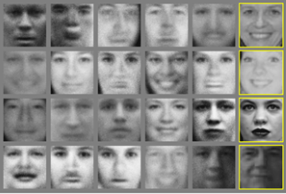
  $p(\mathbf{X})$. This distribution is then sampled to generate new designs that are both similar to designs in the data set overall, yet unique to any particular design in the data set. GNNs learn this distribution automatically through a training process, and thus, automatically parameterize the design space. Moreover, because GNNs learn from a data set of previous designs, they naturally combine features from different designs in novel ways, which supports the emergence of new designs from previous generations (Krish Reference Krish2011). The viability of this approach stems from recent advances in deep neural networks to automatically learn features from dense data representations with thousands of parameters, such as images and 3D models. Figure 1 shows an example from Goodfellow et al. (Reference Goodfellow, Pouget-Abadie, Mirza, Xu, Warde-Farley, Ozair, Courville and Bengio2014) of generated face images to illustrate the ability to maintain similarity to the training set overall without being identical to any image in the training set. The ability to use these ‘raw’ data formats enables the circumvention of the aforementioned manual parameterization task. For these reasons, GNNs offer a unique approach to conceptual CAD.
Example of GNN output from Goodfellow et al. (Reference Goodfellow, Pouget-Abadie, Mirza, Xu, Warde-Farley, Ozair, Courville and Bengio2014). The rightmost column shows the nearest training sample to the neighboring generated sample column. These results demonstrate the two aspects of GNNs desirable for conceptual CAD, diversity of output while maintaining similarity to the training set overall to capture its embedded information.
While GNN research initially focused on image or caption generation problems (Goodfellow et al. Reference Goodfellow, Pouget-Abadie, Mirza, Xu, Warde-Farley, Ozair, Courville and Bengio2014; Radford et al. Reference Radford, Metz and Chintala2015; Dosovitskiy and Brox Reference Dosovitskiy and Brox2016; Sønderby et al. Reference Sønderby, Raiko, Maaløe, Sønderby and Winther2016; Sbai et al. Reference Sbai, Elhoseiny, Bordes, LeCun and Couprie2018), more recently GNN methods for 3D shapes have been developed (Maturana and Scherer Reference Maturana and Scherer2015; Burnap et al. Reference Burnap, Liu, Pan, Lee, Gonzalez and Papalambros2016; Qi et al. Reference Qi, Su, Mo and Guibas2017; Groueix et al. Reference Groueix, Fisher, Kim, Russell and Aubry2018; Liu et al. Reference Liu, Giles and Ororbia2018), coinciding with the availability of large-scale 3D model repositories such as ShapeNet (Chang et al. Reference Chang, Funkhouser, Guibas, Hanrahan, Huang, Li, Savarese, Savva, Song and Su2015) and ModelNet40 (Wu et al. Reference Wu, Song, Khosla, Yu, Zhang, Tang and Xiao2015). There are multiple ways to represent a 3D shape, including voxels, point clouds, polygonal meshes, and through multiple 2D views of the shape. While polygonal meshes tend to be ideal for physics-based simulation, the output of GNNs has been mostly limited to either a voxel-based representation (Maturana and Scherer Reference Maturana and Scherer2015; Liu et al. Reference Liu, Giles and Ororbia2018) or a point cloud (Qi et al. Reference Qi, Su, Mo and Guibas2017; Groueix et al. Reference Groueix, Fisher, Kim, Russell and Aubry2018; Li et al. Reference Li, Zaheer, Zhang, Poczos and Salakhutdinov2018), which can then be transformed into a polygonal mesh via a post-processing step. Point cloud models avoid the memory problem that voxel-based representations suffer from at finer resolutions, as the number of voxels scales cubically with the resolution (Groueix et al. Reference Groueix, Fisher, Kim, Russell and Aubry2018). In contrast, the number of surface points in a point cloud model scales closer to quadratically, as only the surface area of the model is captured by the points. Moreover, sensors that can acquire point cloud data are becoming more accessible such as Lidar on self-driving cars, Microsoft’s Kinect, and face identification sensors on phones (Li et al. Reference Li, Zaheer, Zhang, Poczos and Salakhutdinov2018), allowing large data sets to be easily created.
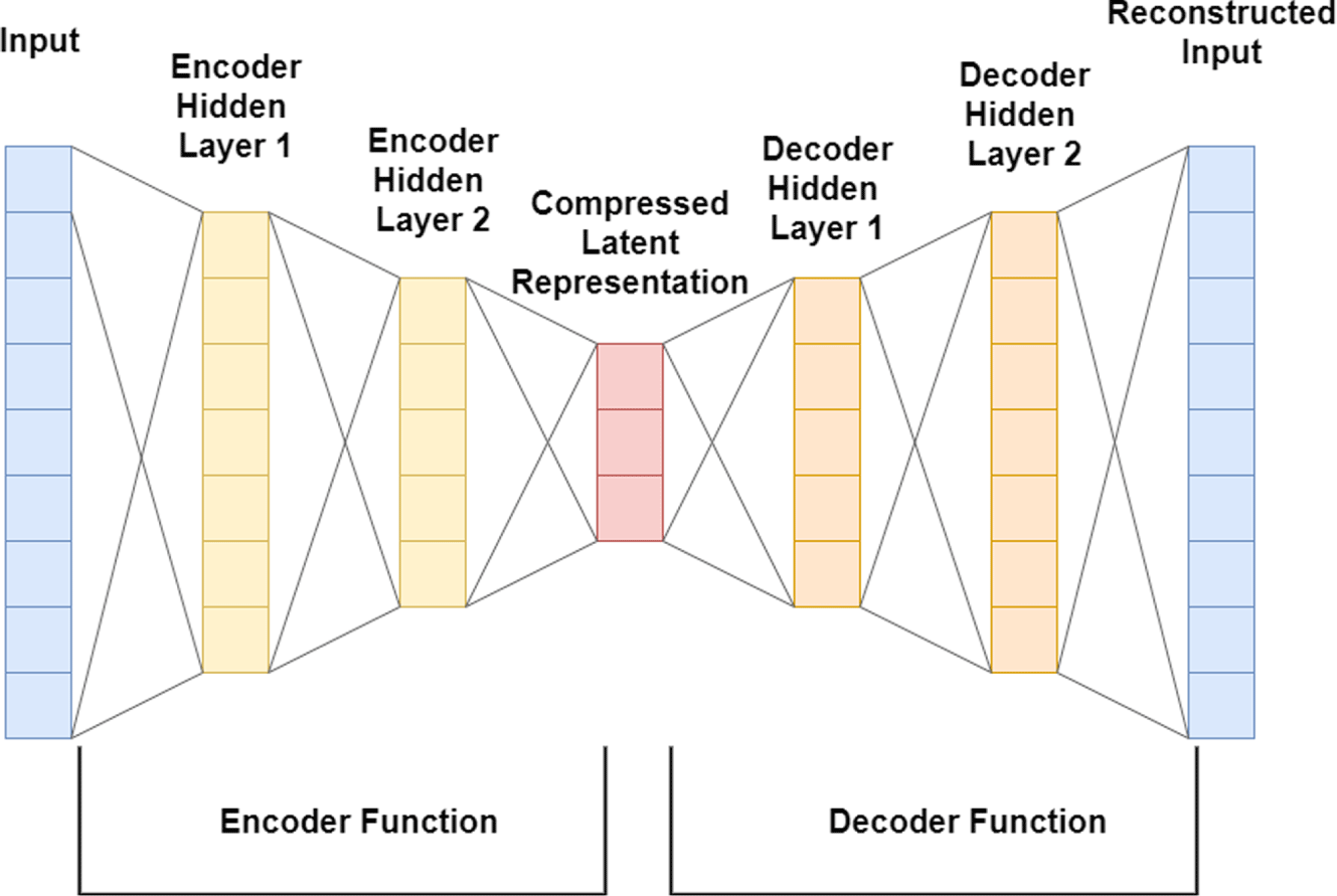
Simplified illustration of the architecture of a deep autoencoder. In reality, there are additional hidden layers, and the hidden layers are themselves often constructed as blocks containing more complex neural network architectures such as ResNet (He et al. Reference He, Zhang, Ren and Sun2016).
While 3D object GNNs have achieved impressive reconstruction results, they are implemented outside of a design context the vast majority of the time. Consequently, generated shapes are typically validated according to their resemblance to objects in the data set, with no physics-based evaluation (Dosovitskiy et al. Reference Dosovitskiy, Springenberg and Brox2015; Wu et al. Reference Wu, Zhang, Xue, Freeman and Tenenbaum2016). In typical contexts in which GNNs are used, the evaluation phase is meant to explore the scope of the learned latent space, and thus sampling the latent space using Gaussian noise or interpolating between different objects in the training data achieves this goal. However, in a design context, in order to effectively transition into the detailed design phase, the latent space must be narrowed down to functionally superior designs (Ulrich Reference Ulrich2003). There is currently a knowledge gap in what optimization strategy would be most effective for improving the functionality of generated designs from state-of-the-art GNNs, without sacrificing the aspects of GNNs that make them appealing in the first place.
GNNs are a group of artificial neural network models that are used to estimate the underlying probability distribution of a data space. Training of GNNs requires a set of samples from a training data set. In practice, the number of samples in the training data set is finite. With a well-trained GNN model as an estimator of the data probability distribution, new samples can be generated from the data space. An example of a data space is the group of all images of a vehicle. In this case, the finite training data set is a finite set of vehicle images. By training a GNN model with such a data set, the user can obtain new images of a vehicle that do not exist in the training data set. Various GNN models have been proposed such as generative adversarial networks (GANs) (Goodfellow et al. Reference Goodfellow, Pouget-Abadie, Mirza, Xu, Warde-Farley, Ozair, Courville and Bengio2014), variational autoencoder (VAE) (Kingma and Welling Reference Kingma and Welling2013), flow-based generative models (Dinh et al. Reference Dinh, Krueger and Bengio2014) and autoregressive generative models (Van den Oord et al. Reference Van den Oord, Kalchbrenner, Espeholt, Vinyals and Graves2016). Among the various GNN models, an autoencoder is chosen by the authors as the generative model for generating 3D designs due to its convenient structure for bijection between the data space of 3D designs and the latent space that is used to specify design parameters. Unlike the popular GAN model, which only takes a latent variable as the input and outputs a 3D design, an autoencoder model uses both an encoder model to convert a 3D design to a latent variable and a decoder model to convert the latent variable back to a 3D design.
The basic design of a deep autoencoder is illustrated in Figure 2. The latent space in this GNN formulation is more amiable to parametric optimization due to the fact that it does not require latent vectors to be normally distributed to produce meaningful results, and latent vectors of designs in the training set can be easily identified using the encoder. The latter aspect allows training data to be used to initialize parametric optimization techniques, which is not suitable in the GAN formulation.
In our previous work (Cunningham et al. Reference Cunningham, Simpson and Tucker2019), we used a pre-trained implementation of the state-of-the-art point cloud generating autoencoder AtlasNet (Groueix et al. Reference Groueix, Fisher, Kim, Russell and Aubry2018) that used a 1024-dimensional latent vector. We noted that when passing a point cloud from the training set through the encoder of this network, the resulting latent vector was on average 64% zeros. This empirical result aligns with Qi et al.’s description of the closely related PointNet (Qi et al. Reference Qi, Su, Mo and Guibas2017) as a deep autoencoder that learns a ‘sparse set of keypoints’ to describe the geometry of a point cloud. Thus, the authors hypothesize that optimization methods that encourage sparsity would result in objects that are more similar to the training data and, as a result, preserve the training set’s embedded design knowledge.
This work proposes a method to generate a diverse set of 3D designs from a point cloud generating autoencoder that will outperform the training data set with respect to some performance metric. A naïve approach would be to use a standard genetic algorithm (GA) to optimize the performance metric over the latent space of a GNN, with the initial population of latent vectors initialized randomly. We refer to this approach as naïve latent space optimization (LSO). However, we hypothesize that this naïve approach would tend to result in a lower-diversity set of designs than a method that specifically exploits the structure of the latent vectors, even when a GA that is well-suited to discovering multiple solutions is used, such as differential evolution (DE) (Li et al. Reference Li, Epitropakis, Deb and Engelbrecht2016).
This work introduces an  $\ell _{0}$ norm penalty to the loss function of the GA, which we refer to in this work as sparsity preserving latent space optimization (SP-LSO). We hypothesize that this modification will encourage sparsity in the output, as well as reduce the likelihood of the GA converging to a single design. We also hypothesize that sparsity is further encouraged by replacing the random initialization of latent vectors in the naïve approach with initialization to the latent vectors of objects from the training set, which we will refer to as training data set initialization (TDI-LSO). The proposed method combines both of these approaches, and thus we refer to it as training data initialized sparsity preserving latent space optimization (TDI-SP-LSO). To highlight the impact of each of these modifications on the LSO task, we compare the proposed method to TDI-LSO and naïve LSO.
We formulate four hypotheses about the performance of the proposed method. The first is that the proposed method will produce designs that are on average functionally superior to designs in the training data set, as quantified by some performance metric.
The second and third hypotheses are that the proposed method will increase the average diversity of point clouds in the output population compared to the naïve approach and the TDI approach, respectively. This can be quantified using a standard similarity metric for point sets such as the Hausdorff distance (Taha and Hanbury Reference Taha and Hanbury2015; Zhanga et al. Reference Zhanga, Lia, Lic, Lina, Zhanga and Wanga2016; Zhang et al. Reference Zhang, Zou, Chen and He2017). The Hausdorff distance between point sets  $A$ and $B$ is defined as
 $$\begin{eqnarray}H(A,B)=\max _{a\in A}\left\{\min _{b\in B}\{d(a,b)\}\right\},\end{eqnarray}$$
 where  $d(\cdot ,\cdot )$ is the Euclidean distance between points $a$ and $b$. Intuitively, it defines the distance between two point sets as the maximum distance of a set to the nearest point in the other set. We would then say that two point clouds with a large Hausdorff distance are dissimilar. Extending this notion to a population of point clouds, we can say that a population is diverse if the average Hausdorff distance between all unique pairs of point clouds in the population is large. This is the method by which the second and third hypotheses are quantified.
The fourth and final hypothesis is that the proposed method will result in a population of designs that is more similar to the training data set than the naïve approach. Once again, similarity is quantified in terms of the Hausdorff distance. Stating each of these hypotheses formally, we have:
- H1.

- H2.
- H3.
- H4.


where
∙
$N$ is the number of point clouds $\mathbf{p}$ in a population of designs $\mathbf{P}$∙
$\mathbf{t}$ is a particular point cloud from the training data set $\mathbf{T}$; these point clouds have the same dimensionality as those in $\mathbf{P}$∙
$L(\cdot )$ is the loss function tied to some performance metric∙ The subscript
$0$ in H1 refers to the initial population for the TDI-SP method, which consists of sample designs from the training set∙
$H(\mathbf{p}_{1},\mathbf{p}_{2})$ is the Hausdorff distance, a standard method for measuring the similarity between two point sets∙ The subscripts TDI-SP, TDI, and naïve refer to the final population of each of these methods.


A realization of the proposed method in a CAD tool would be able to generate 3D models of hundreds of unique candidate conceptual design solutions that are validated with respect to a specific performance criterion. Moreover, these candidate designs would be familiar to the human designer by virtue of their similarity to human-created designs in the training set. The human designer could cycle through these many design candidates until a design is found that sparks inspiration as a creative solution to the problem. The advantage of this method over GNN approaches that do not generate 3D models is that the candidate design is already in a form that is amiable to transition into the detailed design phase, and has been validated with respect to the target performance criteria. This approach is adaptable depending on the needs of the designer in the sense that if a specialized data set for the target application is available, the GNN can be retrained specifically to this data set. Otherwise, a GNN that has been pre-trained on publicly available data sets containing a variety of shapes can be used. Each of these approaches is examined in the experiments conducted in this work.
The key contribution of this paper is the introduction of an  $\ell _{0}$ norm penalty that exploits the fact that deep point cloud generating autoencoders represent 3D objects as a sparse latent vector. Preserving this sparsity improves the diversity of designs generated from LSO, as well as prevent LSO from deviating wildly from objects in the training data set. While this method is proposed with sparse GNN latent spaces in mind, it is applicable to any parametric space where sparsity that exists in the initial population should be preserved. The rest of this paper is organized as follows. Section 2 reviews related literature, Section 3 provides the details of the method, and Section 4 then applies this method to two case studies, a toy example and a practical example. Section 5 discusses results of the experiments and Section 6 provides conclusions of our findings.
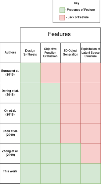
Comparison of features of this proposed method to most closely related literature
2 Related works
In this section, we discuss existing non-GNN-based and GNN-based approaches to conceptual design support, as well as GAs for parametric optimization. Table 1 outlines the features of previous contributions compared to our method.
2.1 Non-GNN approaches to conceptual design support
Shape grammars, first introduced by Stiny and Gips (Reference Stiny and Gips1971) in 1971, are a broad category of methods for design exploration and optimization. Shape grammar methods construct a formal language using a vocabulary of shapes, a set of rules, a set of labels, and an initial shape. The rules are applied recursively to the initial shape until they reach an end point at which no further rule can be applied, and this constitutes a unique shape. Shape grammars were initially popular in the field of architecture, with early incarnations such as the Palladian Grammar (Stiny and Mitchell Reference Stiny and Mitchell1978), the Prairie House Grammar (Koning and Eizenberg Reference Koning and Eizenberg1981), and the Queen Anne House Grammar (Flemming Reference Flemming1987). Shape grammars have been used to generate designs that adhere to a certain ‘brand identity’ (Pugliese and Cagan Reference Pugliese and Cagan2002; McCormack et al. Reference McCormack, Cagan and Vogel2004) as well as interpolate between different classes of designs (Orsborn et al. Reference Orsborn, Cagan, Pawlicki and Smith2006). Shape grammar methods provide users with a flexible method to explore a design space grounded in design constraints as long as a shape grammar has already been constructed for that design space. Creating a shape grammar for a new application is non-trivial, which is a drawback when compared to other methods including the one presented in this work (Gips Reference Gips1999).
Another category of conceptual design support aims to simulate a work flow that involves sketching by hand. Bae et al. (Reference Bae, Balakrishnan and Singh2008) propose ILoveSketch, which is a system to translate virtual 2D sketches into 3D models. Users draw designs from multiple perspectives, and computer vision techniques are used to construct a 3D model out of these perspectives. Kazi et al. (Reference Kazi, Grossman, Cheong, Hashemi and Fitzmaurice2017) propose a method called DreamSketch, which is a 3D design interface that incorporates free-form sketching with generative design algorithms. The user coarsely defines the design problem via a sketch, and then uses topology optimization to generate several 3D objects that satisfy the sketched design constraints. Zoran and Paradiso (Zoran and Paradiso Reference Zoran and Paradiso2013) introduce a 3D Freehand digital sculpting tool. A virtual model of a 3D object is used in conjunction with a custom sculpting device. This device is made to sculpt a block of foam and provide haptic feedback to the user so that the user is able to precisely sculpt the desired object. These methods maximize the designers’ ability to explore their mental representations of designs in a virtual environment, but unfortunately they have not been efficiently implemented such that they can be used in real time to satisfy design constraints (Zboinska Reference Zboinska2015; Kazi et al. Reference Kazi, Grossman, Cheong, Hashemi and Fitzmaurice2017).
Parametric modeling entails reducing the design space into a parameterized form, and then searching over that design space via these parameters. Krish (Reference Krish2011) proposes a framework for conceptual generative designs that starts with using genetic strategies to search over a parameterized design space (which he calls genotypes). Krish acknowledges that many representations should be experimented with, as the choice of representations will impact the quality of the final designs. Practical considerations for integrating this method into CAD software is also discussed. Turrin et al. (Reference Turrin, Von Buelow and Stouffs2011) propose the use of a GA to incorporate performance driven designs into the early exploration of architectural geometry. Bayrak et al. (Reference Bayrak, Ren and Papalambros2016) create a parameterization for hybrid powertrain architectures using a modified bond graph representation, which can then be solved for the optimal powertrain design. These techniques suffer from the drawback that the best parameterization of the design space is not obvious, takes an extensive amount of work to develop, and has a substantial impact on the final result. Our method overcomes this drawback by leveraging the ability of GNNs to automatically learn an effective parameterization of the design space.
2.2 Genetic algorithms for parametric optimization
While manual parameterizations of the design space have their drawbacks, the optimization strategy over the latent space of an autoencoder is not fundamentally different from parametric optimization techniques, and thus literature on this topic is reviewed here. Renner and Ekárt (Reference Renner and Ekárt2003) gives an overview of GAs in CAD with respect to both parametric design and creative design problems. He states that GAs facilitate the combination of components in a novel and creative way, making them a good tool for creative design problems while also having the ability to optimize a parameterized shape with respect to performance criteria. Rasheed and Gelsey (Reference Rasheed and Gelsey1996) discuss modifications to the simple classical implementation of the GA based on binary bit mutation and crossover that are more conducive to solving complex design problems. These modified GAs included parametric GA, selection by rank, line crossover, shrinking window mutation, machine learning screening, and guided crossover. These works motivate the use of GA in a design context, and provide the inspiration for using GA to optimize the latent space of an autoencoder. However, the proposed method improves on these methods further by specifically exploiting the structure of latent vectors in the training set.
Yannou et al. (Reference Yannou, Dihlmann and Cluzel2008) propose an interactive GA system that uses a designer’s subjective impression of each generation as a basis for the fitness function of the algorithm. Poirson et al. (Reference Poirson, Petiot, Boivin and Blumenthal2013) propose another interactive GA technique eliciting user’s perceptions about the shape of a product to stimulate creativity and identify design trends. While the proposed method is agnostic to the fitness function outside of the addition of an  $\ell _{0}$ norm penalty, and thus could in theory be compatible with these methods, there have been other works with GNNs that are specifically geared for this type of subjective evaluation problem (discussed in the following subsection). For these reasons, the proposed method is better suited for fitness functions tied to an objective performance criterion, an area where existing GNN CAD approaches are lacking.
Part of the motivation for introducing an  $\ell _{0}$ norm penalty into the GA cost function is to promote diversity in the output designs. Approaches that focus on finding multiple optimal or near-optimal solutions in a single simulation run are known as niching methods or multi-modal optimization methods. In Li et al.’s survey of niching methods (Li et al. Reference Li, Epitropakis, Deb and Engelbrecht2016), a variety of modified GAs for niching are discussed. One popular GA variant for niching is fitness sharing, in which the fitness function penalizes the fitness of an individual based on the presence of neighboring individuals. Another technique, crowding, relies instead on a competition mechanism between an offspring and its close parents to allow adjusted selection pressure that favors individuals that are far apart and fit. Differential evolution creates offspring using scaled differences between randomly sampled pairs of individuals in the population. This property makes DE’s search behavior self-adaptive to the fitness landscape of the search space and has been shown in other work (Epitropakis et al. Reference Epitropakis, Tasoulis, Pavlidis, Plagianakos and Vrahatis2011, Reference Epitropakis, Plagianakos and Vrahatis2012) to cluster around either global or local optima as the algorithm iterates. Niching methods can be used in conjunction with the proposed method to further promote the discovery of diverse solutions, and for this reason, DE is chosen as the particular GA for LSO in the experiments in this work. Moreover, the $\ell _{0}$ norm penalty introduced in this work also serves to ensure that output designs do not stray too far from human designs, which niching methods alone do not attempt to enforce.
2.3 GNNs for conceptual design support
Before robust GNNs for generating 3D models existed, early work in using GNNs for design leveraged 2D image generating GNNs. Burnap et al. (Reference Burnap, Liu, Pan, Lee, Gonzalez and Papalambros2016) incorporated a VAE into a design context by generating 3D automobile designs. The VAE showed the ability to generate novel models of automobiles that represented specific brands, as well as interpolation between the different brands. However, the authors used crowdsourcing as a functional validation tool as opposed to an objective function evaluation software. A later work by Burnap et al. (Reference Burnap, Hauser and Timoshenko2019) builds on the previous work by using a GNN approach to augment images of human designs to be more aesthetically appealing. However, this approach only generates 2D images and leaves a human designer to determine how to realize the full 3D design in a functionally feasible way. Dering et al. (Reference Dering, Cunningham, Desai, Yukish, Simpson and Tucker2018) propose a method that leverages a VAE model called sketch-RNN to generate 2D designs that are then evaluated in a 2D simulation software. Instead of directly optimizing over the latent space, the authors continually replace designs in the data set with high performing designs from the evaluation software. Chen et al. (Reference Chen, Chiu and Fuge2019) propose a generative model for parameterizing airfoil curves in two dimensions, which are also evaluated in a 2D software. Oh et al. (Reference Oh, Jung, Lee and Kang2018) combine GNNs and topology optimization to optimize the shape of generated images of wheels according to their compliance. Raina et al. (Reference Raina, McComb and Cagan2019) propose a deep learning method to learn to sequentially draw 2D truss designs from a data set of human pen strokes. This approach allows the learning agent to dynamically participate in the design process with a human designer, and is not mutually exclusive with the proposed method that is aimed at providing a human designer with a population of conceptual candidate designs as potential starting points. While these works offer the ability to aid human designers by synthesizing 2D images, extension to 3D models is necessary for GNNs to be feasible in many design applications, and better facilitate a transition into the detailed design phase.
Zhang et al. (Reference Zhang, Yang, Jiang, Nigam, Soji, Furuhata, Shimada and Kara2019) developed a GA-LSO method to improve the gliding height of 3D glider designs using a voxel-based VAE that is modified to generate a lattice of signed distance fields (SDFs). Modifying the voxel output to SDFs allows for the generation of smooth surfaces. Their approach most closely resembles the TDI-LSO approach discussed in Section 1. However, their method also applies two significant restrictions to achieve diversity in the output and similarity to the training set, which are relaxed in this work. Specifically, the authors use a variant of the GA that employs a line crossover restriction; that is, it restricts the combination of parent latent vectors to linear interpolations. This offsets the problem of the naïve GA deviating heavily from the training set by restricting it to linear combinations of objects in the training set, but also limits the GA to discovering a small subset of the total latent space. Second, they use a binary pass/fail performance metric to overcome the challenge of the GA converging to a single-optimal design concept. However, this limits the information provided in the final population of designs, as gliders that surpass the threshold by a wide margin are seen as functionally equivalent to those that narrowly achieve it. Our method is able to overcome the same challenges without applying either of these restrictions through the addition of the  $\ell _{0}$ norm penalty function to the loss function of the GA.
Non-GNN approaches rely on manual parameterization of design spaces, which is not always practical. The use of GNNs in a design context to this point has relied on heavy restrictions such as 2D output or binary performance metrics. Our work overcomes these limitations by proposing a method to enable the use of GNNs in a 3D design context without these restrictions.
3 Method
In this section, we detail our proposed method to sample functionally superior designs from a point cloud generating autoencoder with respect to some performance metric, while maintaining diversity and similarity to the training set in the output.
3.1 Sparsity preserving latent space optimization
We consider the following loss function for the GA:
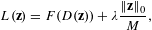 $$\begin{eqnarray}L(\mathbf{z})=F(D(\mathbf{z}))+\unicode[STIX]{x1D706}\frac{\Vert \mathbf{z}\Vert _{0}}{M},\end{eqnarray}$$
where
∙
$L(\cdot )$ is the loss function that is to be minimized∙
$\mathbf{z}$ is the latent representation of the design∙
$F(\cdot )$ is the function implied by the evaluation method, which quantifies design performance∙
$D(\cdot )$ represents the decoder of the AE, as well as the subsequent mesh reconstruction procedure∙
$\Vert \cdot \Vert _{0}$ is the $\ell _{0}$ norm, which is the number of non-zero elements in the vector∙
$\unicode[STIX]{x1D706}$ is the scalar weight of the norm penalty∙
$M$ is the length of the latent vector $\mathbf{z}$.


Flow diagram of how the loss function is calculated from a latent variable  $\mathbf{z}$, as detailed in Equation (2).
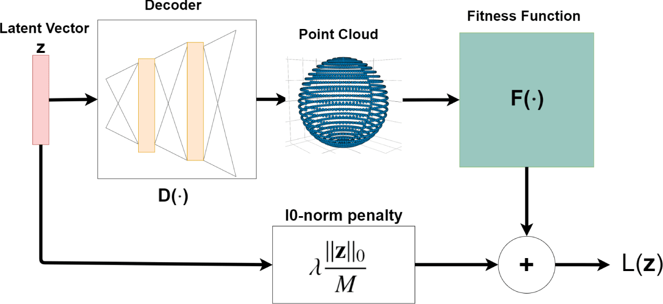
Figure 3 illustrates how this loss function is calculated. The hyperparameter  $\unicode[STIX]{x1D706}$ that is most effective is highly application dependant, and will vary based on the range of $F(\cdot )$ and the average sparsity ratio of latent vectors in the training set being utilized. A hyperparameter search over a range such that neither the sparsity penalty nor the evaluation function is completely dominated by the other is recommended.
A GA is used to search the latent variable space  $\mathbf{Z}$ in order to minimize $L(\mathbf{z})$. GAs refer to a family of computational models that have been used in a wide variety of applications to optimize black-box functions (Whitley Reference Whitley1994). For the purposes of this approach, we will refer to any algorithm that applies crossover, mutation, and selection as a GA, and show through an examination of the DE implementation applied in this method that the expected natural loss of sparsity can be mitigated using an $\ell _{0}$ norm penalty.
3.2 Differential evolution
The details of the DE implementation used in this work are given in Algorithm 1.

We are interested in examining how the average sparsity of vectors in the population is expected to change from one generation to the next. Let the sparsity ratio of a vector  $\mathbf{z}$ be defined as $r=1-(\Vert \mathbf{z}\Vert _{0}/M)$. The quantity we are then interested in is the expected value of the sparsity ratio of $\mathbf{z}^{\prime }$ in Algorithm 1. First, we can say that the expected value of the sparsity in any given vector from generation $g$ is the average sparsity ratio of all vectors in the population $\mathbf{P}_{g}$, which we denote by $r_{g}$.
Continuing with Algorithm 1, the expected sparsity ratio of  $\mathbf{z}_{\text{diff}}$ must be calculated next. Given that the elements of $\mathbf{z}$ are continuous, $z_{\text{diff}}(i)=0$ with non-zero probability only when both $z_{2}(i)$ and $z_{3}(i)$ are 0. Furthermore, throughout this analysis, we will treat the values of vector elements as independent from other vectors in the population, and assume that all elements of a given vector are equally likely to be zero (which is equivalent to saying that each element is 0 with probability $r$). For the expected sparsity ratio of $\mathbf{z}_{\text{diff}}$, we have
 $$\begin{eqnarray}E[r_{\text{diff}}]=\frac{1}{M}\mathop{\sum }_{i=0}^{M}P[z_{3}(i)=0]P[z_{2}(i)=0]=\frac{1}{M}\mathop{\sum }_{i=0}^{M}r_{g}^{2}=r_{g}^{2}.\end{eqnarray}$$
 Continuing through Algorithm 1, the expected sparsity ratio of  $\mathbf{z}_{\text{donor}}$ must be determined. It can be easily shown by the same method as Equation (3) that the resulting expected sparsity ratio is $r_{\text{donor}}=r_{g}^{3}$.
Now the expected sparsity ratio of  $\mathbf{z}^{\prime }$ after recombination can be calculated as
 $$\begin{eqnarray}E[r^{\prime }]=\frac{1}{M}\mathop{\sum }_{i=0}^{M}cP[z_{\text{donor}}(i)=0]+(1-c)P[z(i)=0]=cr_{g}^{3}+(1-c)r_{g}.\end{eqnarray}$$
 This result tells us how the sparsity of vectors in the population degrades when the fitness function  $F(\mathbf{z})$ has no dependence on the sparsity of $\mathbf{z}$. For example, with a recombination rate of $c=0.75$ and a sparsity ratio in the current generation of $r_{g}=0.6$, we will have $E[r^{\prime }]=0.312$. Therefore, any newly created vectors that are introduced into the population will be expected to have approximately half the sparsity of vectors from the previous generation.
However, when an  $\ell _{0}$ norm penalty is introduced into the fitness function, the more the sparsity lost by a particular vector $\mathbf{z}^{\prime }$, the less likely that the vector is to be included in the next generation’s population, proportional to the penalty weight $\unicode[STIX]{x1D706}$.
A critical feature to note with this method is that it does not produce a population of vectors with higher sparsity than the previous generation. In the case where the fitness function is nothing but the  $\ell _{0}$ norm penalty, the sparsity will stay the same as no new vectors will be introduced into the population. This method preserves sparsity by slowing its natural decay in evolutionary optimization.
In our proposed method, the sparsity in the initial population comes from the encoded latent vectors in the training set. However, a naïve implementation would typically sample the initial population randomly, and thus lack this sparsity in the initial population. For this reason, there is no benefit to applying the  $\ell _{0}$ norm penalty in conjunction with the naïve approach.
4 Application and evaluation
In this section, we investigate the effectiveness of TDI-SP-LSO compared to benchmark test cases that do not use components of our method. We implement two test cases: a toy problem of generating ellipsoid point clouds subject to an evaluation function based on their shape and a practical test case of generating watercraft models where  $F(\cdot )$ is the coefficient of drag. To promote reproducibility, the source codes for the experiments in this work have been published online.Footnote 1
4.1 Ellipsoid case study
This simple test case is included in order to gain an intuition about the proposed method and easily visualize the benefits in design performance and diversity that it offers. Consider a design space of ellipsoids with  $x$ and $y$ radii in the range $[0,10]$ and a fixed $z$ radius of 10. Additionally, consider that the performance metric for each ellipsoid is dictated by its $x$ and $y$ radii as shown in Figure 4, where a higher score is better. Note that there are four separate regions that achieve optimal performance.
Performance function of the ellipsoid design space.
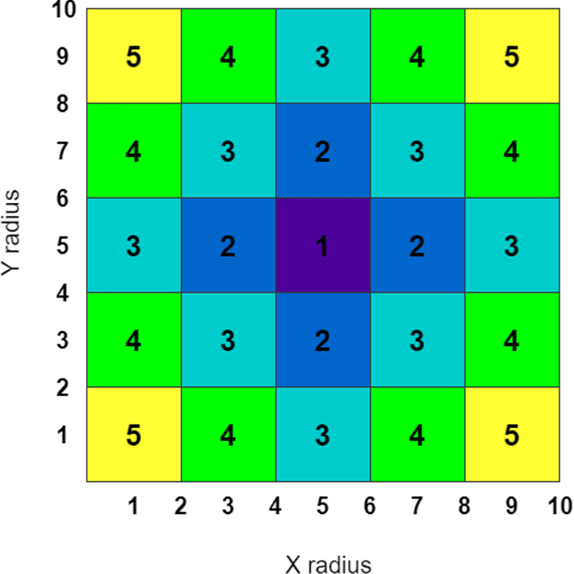
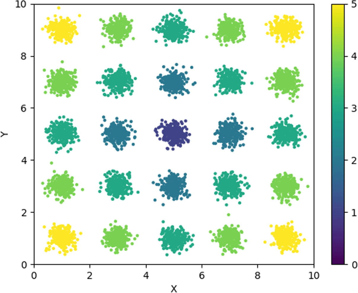
Figure 5 shows the performance distribution of the training data set constructed for this case study. There are 25 Gaussian distributed clusters corresponding to each region of the design space. Each cluster was sampled 250 times for a total of 6250 designs in the data set.
Distribution of training data.
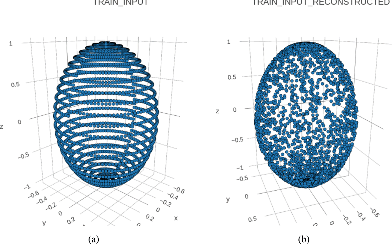
Once this data set was constructed, AtlasNet was trained to learn a 1024-dimensional latent space representation from which it could accurately reconstruct ellipsoids from the training data set. Reconstruction results from AtlasNet after 120 epochs of training on the ellipsoid data set are shown in Figure 6. The reconstructed ellipsoid is accurate with respect to the overall shape of the original, but the finer structures of the point arrangements are lost. This is consistent with state-of-the-art point cloud reconstruction results (Qi et al. Reference Qi, Su, Mo and Guibas2017; Groueix et al. Reference Groueix, Fisher, Kim, Russell and Aubry2018).
(a) Sample ellipsoid point cloud from the training data set. (b) AtlasNet’s reconstruction of this ellipsoid after 120 epochs of training on the ellipsoid data set.
Once AtlasNet has been retrained on the ellipsoid data set, the decoder can be used to generate ellipsoid point clouds from 1024-element latent vectors. The performance of these ellipsoids can then be determined by finding the minimum bounding ellipsoid of the generated point cloud, and taking its  $x$ and $y$ radii. In order to frame this as a minimization problem, the loss function for this problem is defined as
 $$\begin{eqnarray}\min _{\mathbf{z}}L(\mathbf{z})=\min _{\mathbf{z}}\left(\frac{1}{P_{\mathbf{z}}}+\unicode[STIX]{x1D706}\frac{\Vert \mathbf{z}\Vert _{0}}{M}\right),\end{eqnarray}$$
 where  $P_{\mathbf{z}}$ is the performance function defined in Figure 4 for the reconstructed point cloud decoded from latent vector $\mathbf{z}$.
This toy problem is useful for validating the proposed method because the performance landscape over the design space is very simple and the optimal solutions are known a priori.
4.2 Watercraft case study
First, the data set of watercraft on which the GNNs were trained is described, then the simulation environment for calculating the drag force is detailed, and finally the experiments discussed in this work are described.
4.2.1 3D model data set
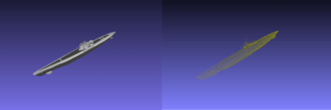
The data set used for this experiment was derived from the ShapeNet data set (Chang et al. Reference Chang, Funkhouser, Guibas, Hanrahan, Huang, Li, Savarese, Savva, Song and Su2015). Specifically, 3879 models from the watercraft category were sampled to create our data set. This category of ShapeNet includes both submarine watercrafts and watercrafts that operate at the interface (e.g. boats), and within those categories the designs vary widely in their intended function. In our experiments, this data set is sampled indiscriminately in order to demonstrate the ability of the proposed method to extract functional designs without the need for careful pruning of an existing data set. Figure 7 shows an example of an object from the data set in both point cloud and mesh format. A pre-trained AtlasNet encoder made publicly available by Groueix et al. (Reference Groueix, Fisher, Kim, Russell and Aubry2018) was used to convert the 3D models into latent vectors of size 1024.
Sample of mesh (left) and corresponding point cloud (right) models from the watercraft data set.
4.2.2 Objective function
The equation for the drag coefficient of a 3D object is as follows:
 $$\begin{eqnarray}C_{D}=\frac{2F_{D}}{\unicode[STIX]{x1D70C}\unicode[STIX]{x1D707}^{2}A},\end{eqnarray}$$
where
∙
$C_{D}$ is the drag coefficient∙
$F_{D}$ is the drag force generated by fluid flow∙
$\unicode[STIX]{x1D70C}$ is the density of the fluid∙
$\unicode[STIX]{x1D707}$ is the flow speed of the fluid∙
$A$ is the 2D-projected area of the object, which is perpendicular to the fluid flow.


Because  $\unicode[STIX]{x1D70C}$ and $\unicode[STIX]{x1D707}$ are constants for all models, we only need to calculate the ratio $R=F_{D}/A$ to get a value that is proportional to the coefficient of drag for each model. Therefore, the optimization problem is cast as
 $$\begin{eqnarray}\min _{\mathbf{z}}L(\mathbf{z})=\min _{\mathbf{z}}\left(R_{\mathbf{z}}+\unicode[STIX]{x1D706}\frac{\Vert \mathbf{z}\Vert _{0}}{M}\right),\end{eqnarray}$$
 where  $R_{\mathbf{z}}$ is the value $R$ returned by the evaluation environment for a particular latent vector $\mathbf{z}$.
4.2.3 Evaluation environment
This section describes the evaluation environment that returns the  $R$ value for a polygonal mesh model. The environment was created using NVIDIA FLeX 1.10, a smoothed-particle hydrodynamics fluid simulation library developed by NVIDIA for both Unity and unreal real-time engine platforms. It provides GPU accelerated fluid, cloth, and soft body real-time simulation (NVIDIA Gameworks 0000). FLeX has been used in both robotics simulation (Collins and Shen Reference Collins and Shen2016; Guevara et al. Reference Guevara, Taylor, Gutmann, Ramamoorthy and Subr2017) and medical simulations (Camara et al. Reference Camara, Mayer, Darzi and Pratt2016, Reference Camara, Mayer, Darzi and Pratt2017; Stredney et al. Reference Stredney, Hittle, Medina-Fetterman, Kerwin and Wiet2017). However, FLeX fluid simulation is intended for real-time visual effects, and thus is a reduced accuracy tool compared to high fidelity CFD software. However, due to time constraints concerning the several trials and variations of the proposed method conducted in our experiments, FLeX was chosen for its ability to run in real time and greatly reduce the run time of our several experiments.
The Unity real-time (Juliani et al. Reference Juliani, Berges, Vckay, Gao, Henry, Mattar and Lange2018) engine has grown from an engine focused on video game development to a flexible general-purpose physics engine, which is used by a large community of developers for a variety of interactive simulations, including high-budget console games and AR/VR experiences. Because of its flexibility and ability to run in real time, Unity is being used as a simulation environment development platform for many research studies (Burda et al. Reference Burda, Edwards, Pathak, Storkey, Darrell and Efros2018; Jang and Han Reference Jang and Han2018; Namatēvs Reference Namatēvs2018). It also includes a robust native physics engine (NVIDIA’s PHYSX) as well as support for custom physics supplements that can be acquired easily from the Unity asset store to which thousands of developers contribute.
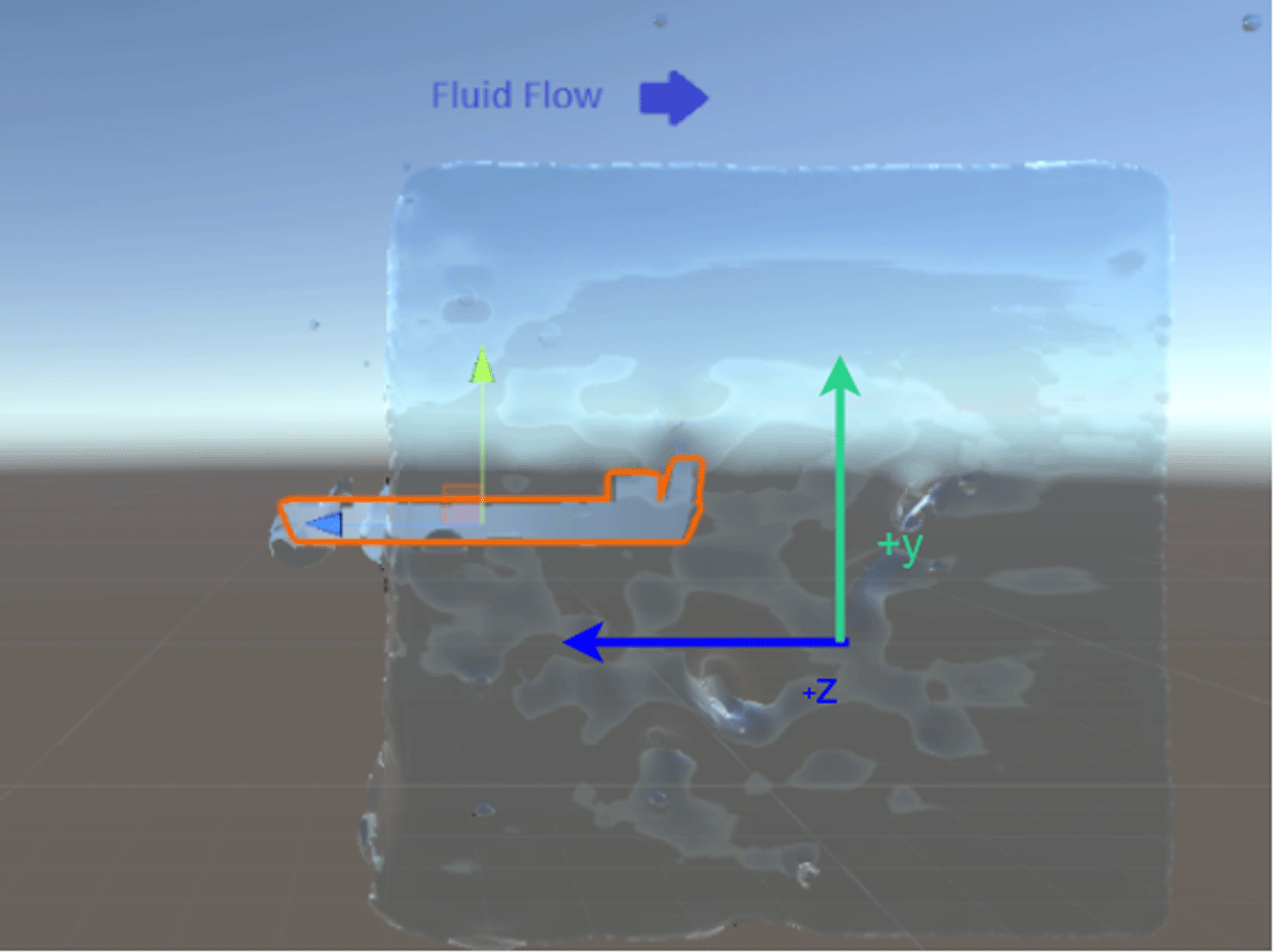
We develop a drag force evaluation environment in Unity by placing the generated object at the center of a cube of 80 000 fluid particles, which are moving toward the object along the negative  $z$ axis, as shown in Figure 8.
Fluid simulation environment for calculating drag coefficient.
At each step of the simulation, the acceleration of the object in the  $z$ direction is calculated. Each object’s mass is calculated according to the assumption that every object is made of material of the same density. The average acceleration is calculated over the course of the simulation, and this value is multiplied by the mass of the object to return the average drag force. Next, we detail the method for calculating the 2D-projected surface area of the object.
4.3 Mesh generation
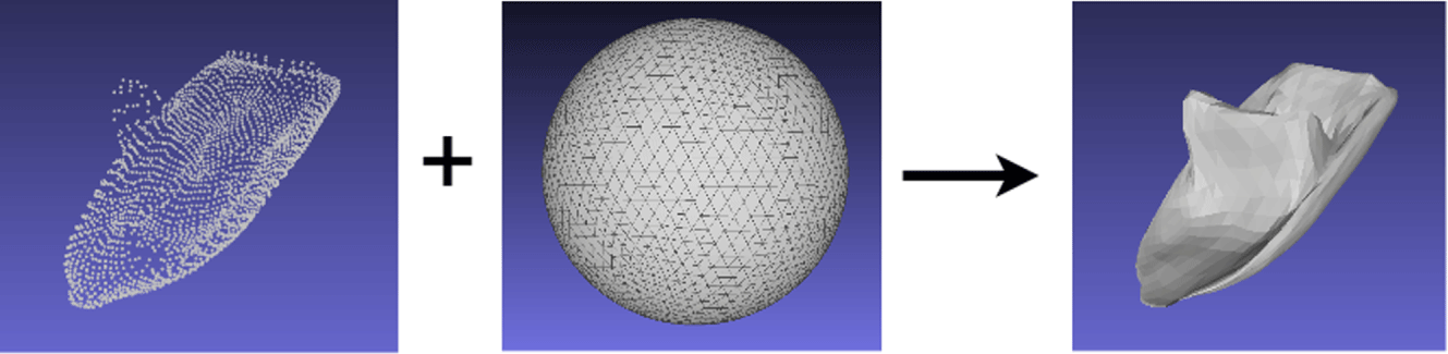
Once point clouds have been generated, they must be converted into a polygonal mesh to be validated with respect to many physics simulations. AtlasNet also provides functionality for mesh reconstruction. Constructing a mesh from a point cloud can be thought of as deciding how to connect a set of vertices to create a smooth surface. AtlasNet’s generated point clouds have a fixed number of vertices that are chosen to be the same as the number of vertices in a reference sphere pictured in Figure 9. The generation of the point cloud can be thought of as morphing the reference sphere by transforming the position of each of its surface points, yet maintaining the same connectivity. Therefore, by using the generated point cloud as the vertices and the sphere’s face connectivity information, the mesh corresponding to the generated point cloud is constructed.
Flow diagram of the mesh reconstruction process.
4.3.1 Surface area projection
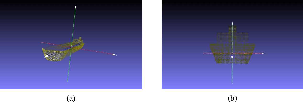
Because the fluid flow is set to arrive from the positive  $z$ axis in the fluid simulation environment, projecting the 3D point cloud to a 2D point cloud is done by setting the $z$ coordinate of each of the points to 0. Figure 10 shows an example of this process.
View of 3D model prior to projection onto 2D plane. Fluid flow is from  $z$ axis. Projection of 3D model onto 2D plane perpendicular to fluid flow.
Once the 2D-projected point cloud has been created, we calculate the area of this point cloud by using the face connectivity information in the 3D mesh, which lists the three vertices in each triangular face of the 3D mesh model. Using the corresponding vertices in the 2D-projected point cloud, the areas of each triangle are calculated and summed together. Then this sum is divided by 2 to account for surfaces in the rear of the object relative to the fluid flow to give the projected area of the object. Combining this quantity with the drag force calculated in the previous section, we are able to calculate  $R_{\mathbf{z}}$ in Equation (7).
This test case evaluates the proposed method with respect to a real design scenario, and an autoencoder that has been pre-trained on a diverse shape data set that is not specialized to the target application.
5 Results and discussion
In this section, we examine the results of the case studies outlined in Section 4, particularly with respect to our hypotheses in Section 1. Each of the following benchmarks is implemented in order to evaluate the proposed method against approaches that remove some of its features.
(1) TDI-SP-LSO (proposed method): The initial population is created by sampling the training data set, and an
$\ell _{0}$ norm penalty is applied to the cost function.(2) Benchmark 1 (TDI-LSO): The initial population of the GA is sampled from the training data set, but the
$\ell _{0}$ norm penalty is applied to the cost function.(3) Benchmark 2 (Naïve): DE is applied with random initialization and no
$\ell _{0}$ norm penalty.


First, we analyze the results of the ellipsoid case study and then the watercraft case study, before tying the analyses of both case studies together and reexamining the hypotheses in Section 1.
For both case studies, multiple trials for each benchmark and the proposed method are run. The initial population of vectors is held constant for a given trial across benchmarks for a fair comparison, but is changed from trial to trial. The DE algorithm is used for LSO with a recombination rate of 0.9 and a mutation rate of 0.05, and run for a total of 35 generations. For all sparsity preserving methods, a hyperparameter search is performed for multiple  $\unicode[STIX]{x1D706}$ values.
5.1 Ellipsoid case study
For this case study, each population consists of 120 latent vectors. Given that the performance landscape is known a priori to have four optimal regions with a performance of  $1/P_{\mathbf{z}}=0.2$, the lambda values of 0.1, 0.2, and 0.4 were chosen for the hyperparameter search. These values correspond to cases where the $\ell _{0}$ norm penalty is weighed half as much as the optimal performance, equal to the optimal performance, and twice as much as the optimal performance, respectively.
Performance evolution for each method averaged across all trials with shaded 0.95 confidence interval.
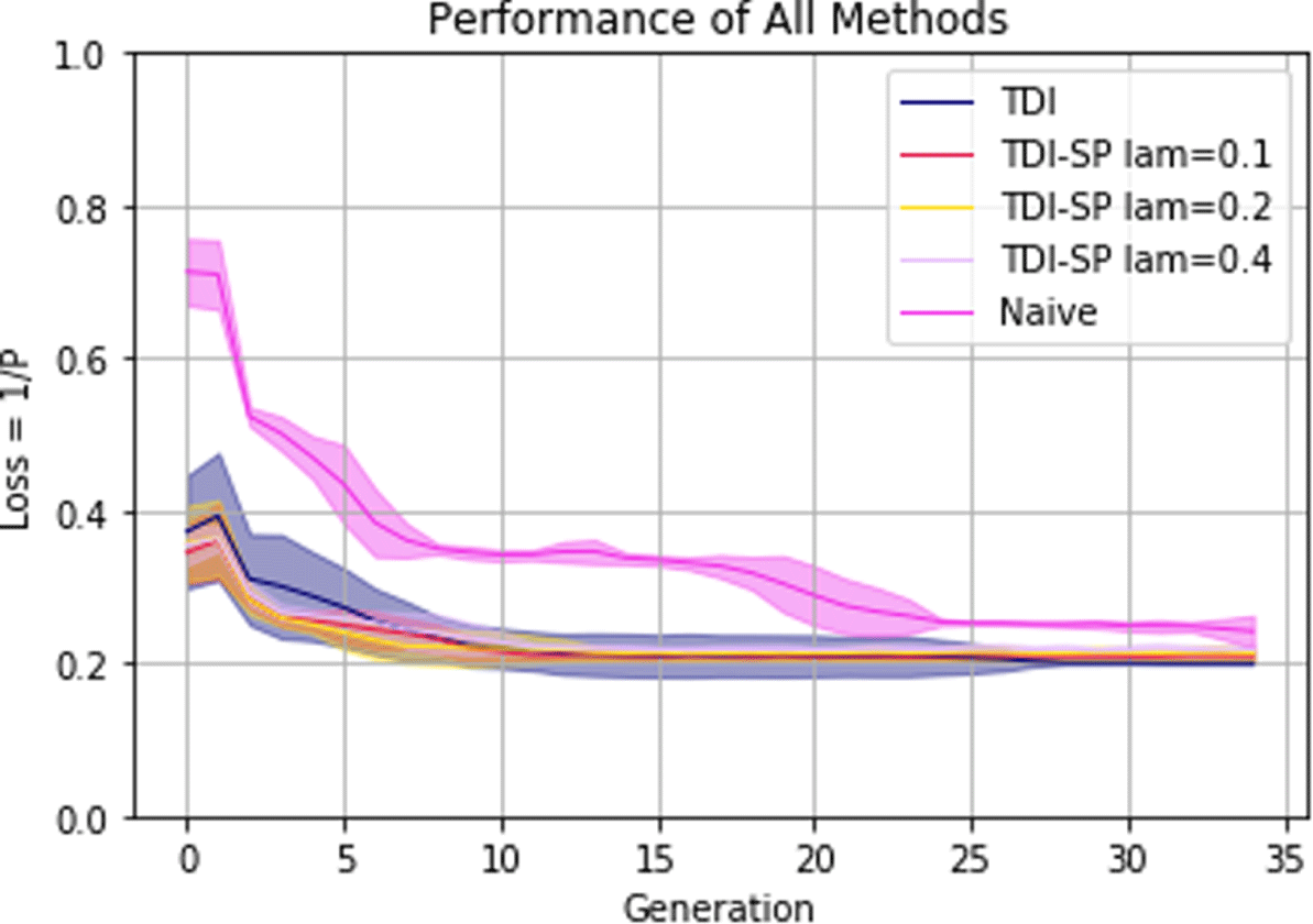
Figure 11 shows the performance curve over the 35 DE steps for each method. The curves shown are the averages for each method across all five trials with a shaded 0.95 confidence interval. Figure 11 makes it clear that data initialization has a dominant effect on the learning curve of the loss, but both methods eventually converge to optimal or near-optimal performance. The improved initial performance of the TDI methods is to be expected based on the assumption that designs in the training data set perform better than a purely random set of parameters. This finding lends support to the claim that performance knowledge is embedded in the training data set, even for a toy problem such as this test case.
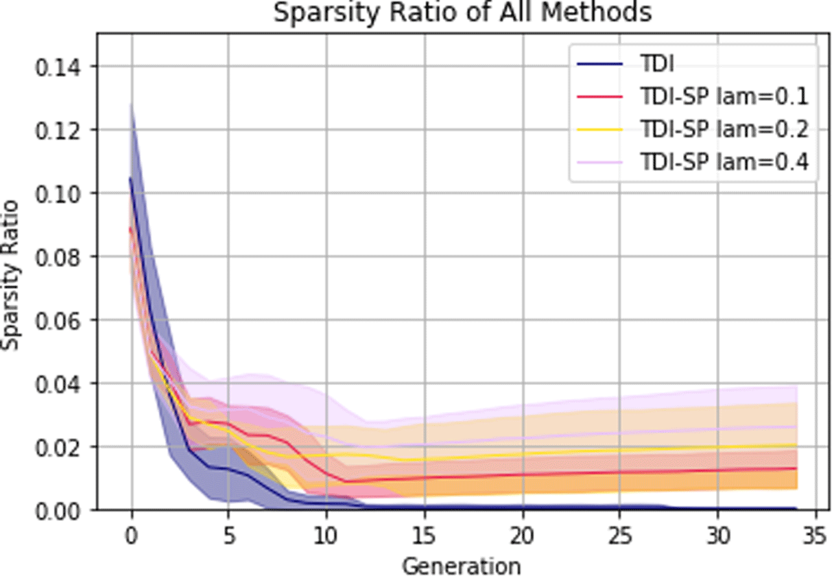
Sparsity evolution averaged across all trials for each TDI method with shaded 0.95 confidence interval. The naïve method is omitted due to it having a sparsity ratio of 0 at all times.
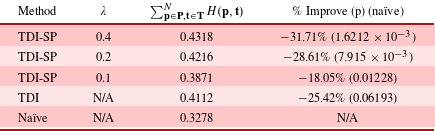
In order to evaluate H1, we compare the performance of the 120 designs in the initial and final populations. The values displayed in Table 2 are the averages of these values across the five trials for each method. We can see that in all of the benchmark methods and the proposed method, the final generation’s average performance is significantly improved compared to the initial generation. Therefore, these results support H1, that is, the proposed method results in functionally superior designs on average compared to sampling the training data set randomly.
(H1) Average difference between average scores of initial and final populations for each method across all trials. Percentage improvement and  $p$-values are calculated between the initial and final generations for each method
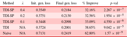
Figure 12 shows how the sparsity ratio of the latent vectors changes as the DE optimization process runs. The fact that the naïve method never produces a population of latent vectors with average sparsity greater than 0 shows that initializing with sparse latent vectors from the data set is critical to enforce sparsity in the final solution set. We can also observe that the sparsity at the end of the curve increases with  $\unicode[STIX]{x1D706}$ although there are diminishing returns going from 0.2 to 0.4 compared to 0.1 to 0.2. Also worth noting is that the sparsity ratio of latent vectors in the training set is only 11% on average compared to 64% for the pre-trained ShapeNet AtlasNet latent vectors. This shows the versatility of the method for multiple application domains that may result in varying sparsity ratios for the training set.
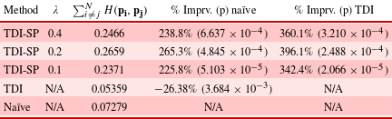
(H2 and H3) Average mean Hausdorff distance across the five trials for different point clouds within the final set of designs  $\mathbf{P}$ for each method. The TDI percentage improvement and $p$-value are calculated with respect to the naïve method, and the TDI-SP percentage improvement and $p$-values are calculated with respect to both the naïve method and the TDI method.
(H4) Average mean Hausdorff distance across the five trials between point clouds in training data set  $\mathbf{T}$ and point clouds of final generation of each method $\mathbf{P}$. Both percentage improvement and $p$-values are calculated with respect to the naïve method.
In order to evaluate H2 and H3, we examine the mean Hausdorff distance across trials between point clouds in the same population for each method, which, as discussed in Section 1, is a standard similarity metric between two point sets. H2 and H3 claim that the proposed method will lead to a set of solutions with more diversity than the benchmarks of the naïve and TDI methods, respectively. In terms of the Hausdorff distance, a larger distance between point clouds within the solution set indicates more diversity. From Table 3, we can see that the proposed method significantly improves in this regard over both the TDI and naïve approaches. This evidence strongly supports both H2 and H3.
Distribution of the 120 ellipsoids in the final generation for each method. The top row shows the initial population for each trial, which was held constant for each method.
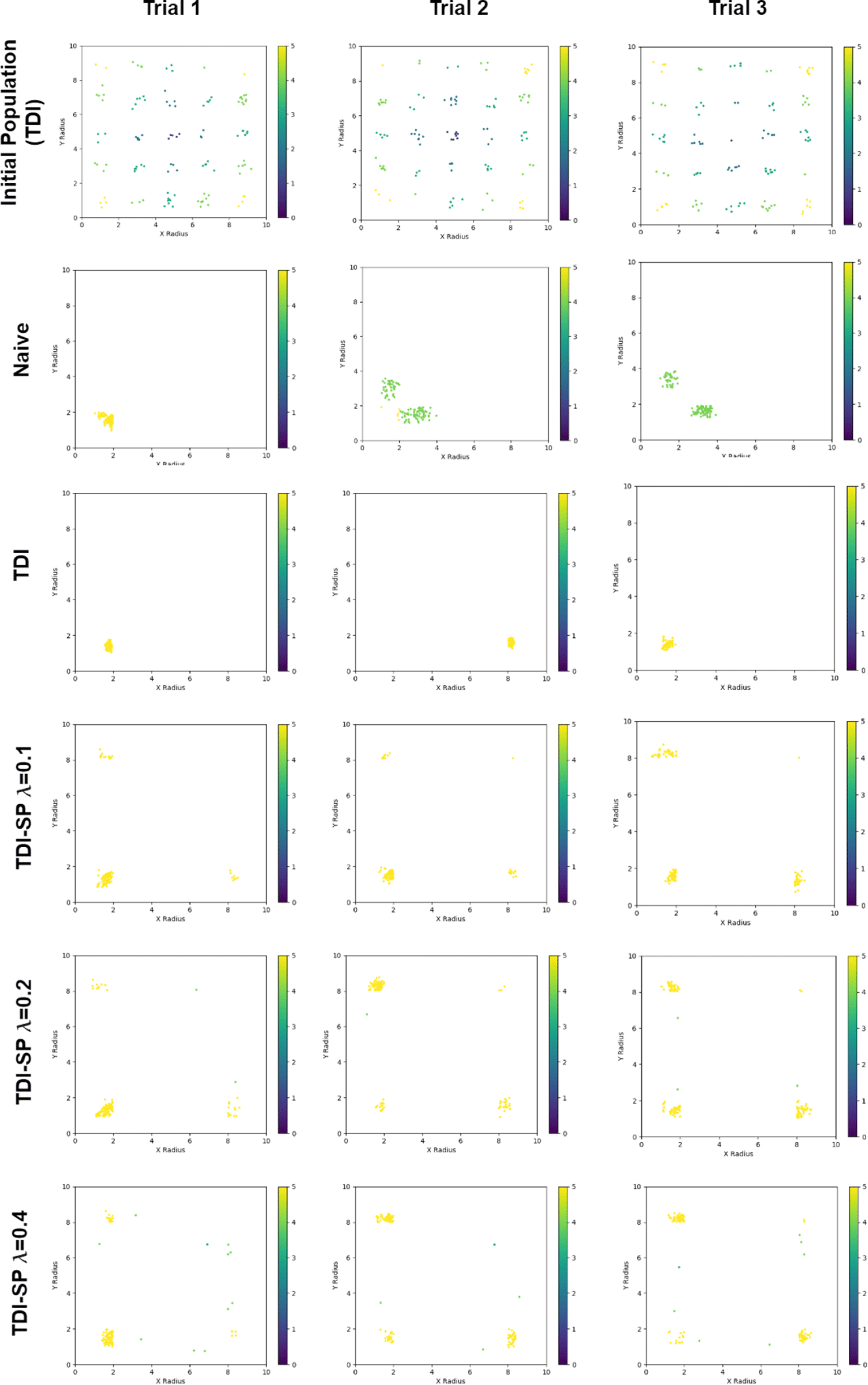
Because of the simply defined performance space of this toy example, we can also easily examine the diversity in the solution space visually. Figure 13 shows the distribution of the final solution set generated by each method, compared to the initial population for the TDI methods for the first three trials. From these plots, we can see that non-sparsity-preserving methods converge at or near only one of the optimal regions for each trial. By contrast, the proposed sparsity preserving method discovers at least three of the four optimal regions in every trial for all choices of  $\unicode[STIX]{x1D706}$. The choice of $\unicode[STIX]{x1D706}=0.1$ results in the highest performing solution set as is expected, but concentrates more in a single cluster compared to the higher $\unicode[STIX]{x1D706}$ values. At the other end, $\unicode[STIX]{x1D706}=0.4$ ensures a diverse population, with the sacrifice of more sub-optimal designs in the population. This visualization confirms in an intuitive manner the findings from the Hausdorff similarity metric, that is, the proposed sparsity preserving method improves design diversity in the solution set.
In order to examine H4, we observe the Hausdorff distance between generated point clouds in the final generation for each method and point clouds in the training data set. In this case, the proposed method was predicted by H4 to have a greater similarity (and a correspondingly lesser Hausdorff distance) to the training set than the benchmark methods. Table 4 shows that the naïve method has a lesser distance to the training set than all other methods, including the proposed method. This is a surprising result that contradicts the prediction of H4.
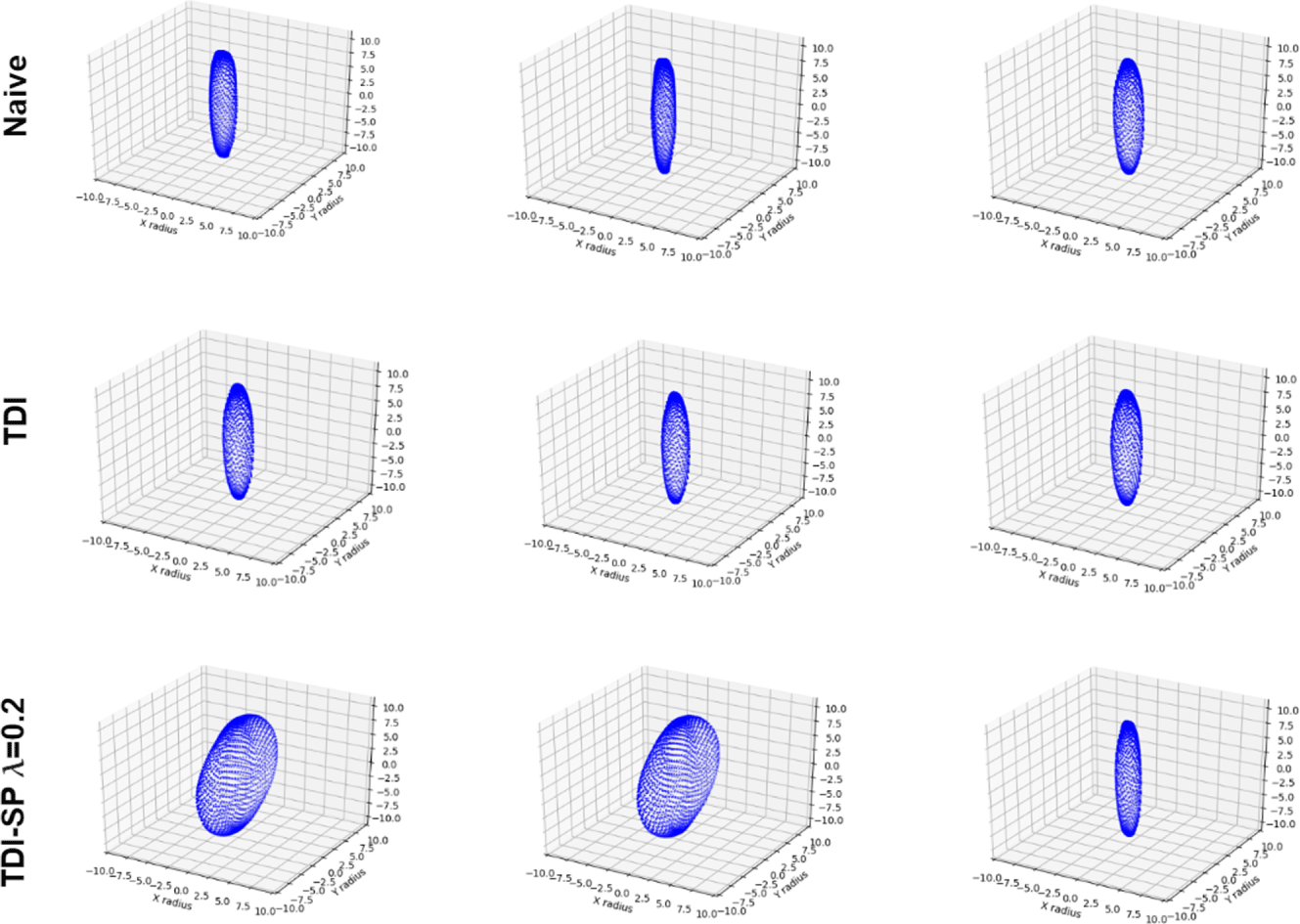
In order to gain an intuitive sense of these and other differences between the point clouds generated with each of these methods, we show three randomly sampled designs from the solution set of each method in the first trial in Figure 14. We can see from these samples that the proposed method shows samples from multiple shape clusters, while the other methods only display very similar shapes from the same cluster. Moreover, we can see a curious feature in the bottom left and bottom middle ellipsoids that may explain the training set dissimilarity of these methods. All ellipsoids in the training set are oriented with their z radius exactly aligned with the  $z$ axis. However, we see in the bottom row that two of the ellipsoids are rotated with respect to this axis, and this could explain the increased Hausdorff distance to the training set.
(Top) Three randomly sampled designs from naïve method. (Middle) Three randomly sampled designs from TDI-LSO method. (Bottom) Three randomly sampled designs from the proposed TDI-SP-LSO method ( $\unicode[STIX]{x1D706}=0.2$). All samples are taken from the first trial.
5.2 Watercraft case study
For this case study, only three trials and a smaller population size of 50 were used due to the increased complexity of the fitness function evaluation step. Two  $\unicode[STIX]{x1D706}$ values are investigated that are proportional to the range of values produced by the fitness evaluation, $5\times 10^{-5}$ and $1\times 10^{-4}$.
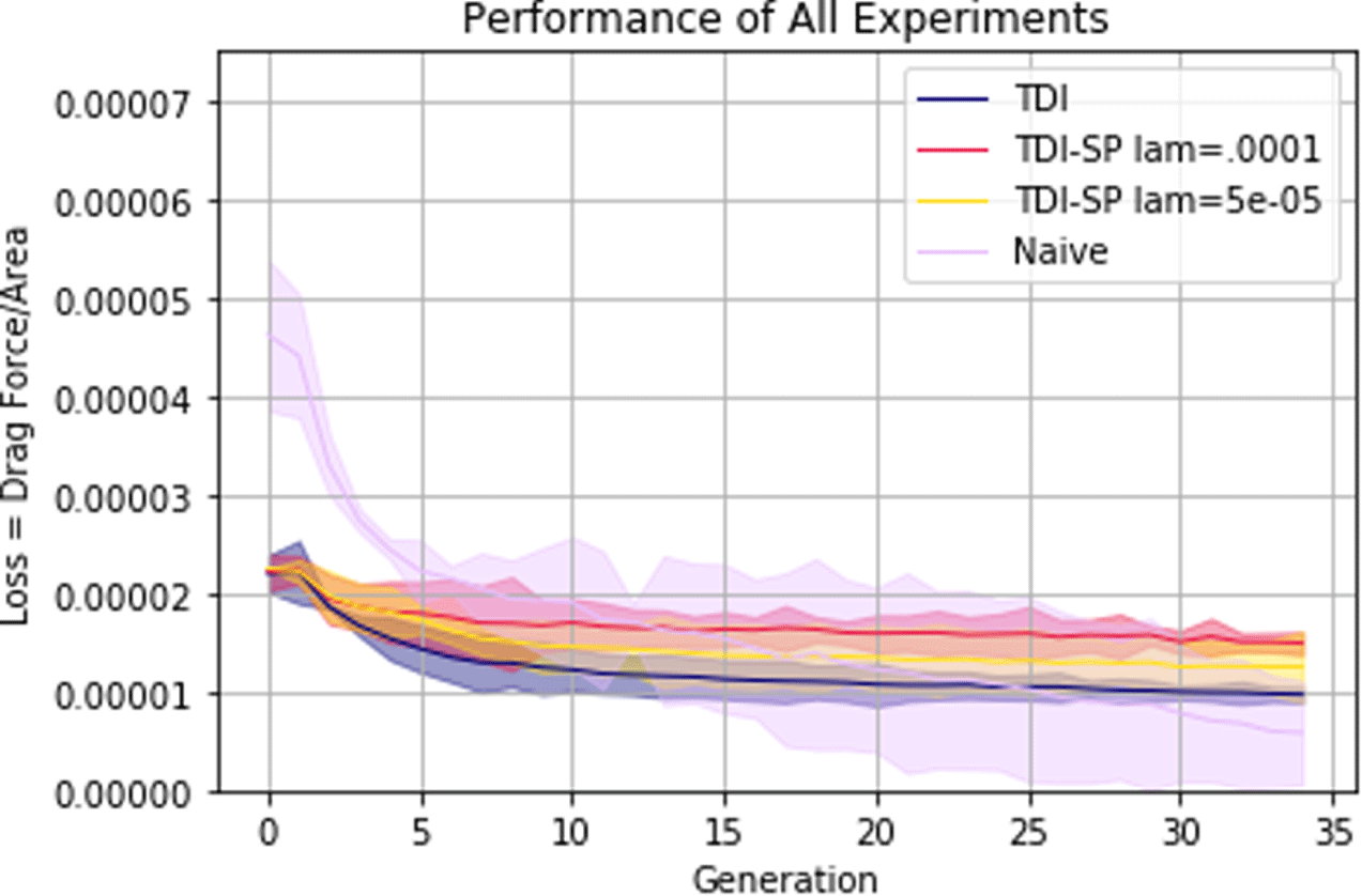
Figure 15 shows the average evolution of the mean  $R$ value across the three trials for each of the methods with a shaded 0.95 confidence interval. The TDI methods are separated by the $\unicode[STIX]{x1D706}$ parameter. As in the previous case study, Figure 15 shows that the data initialization has a dominant effect on the learning curve of the loss, but both methods eventually converge to a similar performance. We can also see a larger gap between the performance of TDI methods and the naïve randomly initialized method. This makes sense given that the data set consists of objects that are designed to have a low drag coefficient.
Evolution of the drag ratio,  $R$, for each method averaged across all trials with shaded 0.95 confidence interval.
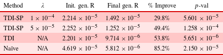
In order to evaluate H1, we compare the average drag ratio,  $R$, of the 50 designs in the initial and final populations. The values displayed in Table 5 are the averages of these values across the three trials for each method. We observe from Table 5 that for all methods, the final performance is improved by a statistically significant margin, the same as in the previous test case. In the case of TDI-SP-LSO with $\unicode[STIX]{x1D706}=1\times 10^{-4}$, the $p$-value between the distribution of performances in the initial and final populations is $5.601\times 10^{-5}$. Therefore, these results support H1, that is, the proposed method results in functionally superior designs compared to sampling the GNN directly.
(H1) Average difference between average scores of initial and final generations for each method across the three trials. Percentage improvement and  $p$-values are calculated between the initial and final generations for each method.
Sparsity evolution averaged across all trials for each TDI method with shaded 0.95 confidence interval. Naïve is omitted due to it having a sparsity ratio of 0 at all times.
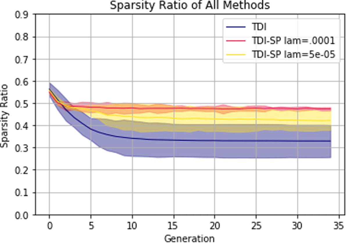
Figure 16 shows how the sparsity of the output changes over the GA optimization process. Contrasting this to Figure 12, we can see that the sparsity is significantly higher when using the AtlasNet weights that had been pre-trained using ShapeNet. This figure also confirms the finding that the  $\ell _{0}$ norm succeeds in preserving sparsity in the final generation.
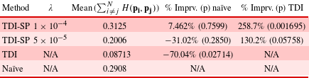
Just as in the previous test case, we examine the mean Hausdorff distance across trials between point clouds in the same population for each method. Table 6 shows that the TDI-SP-LSO diversity is not significantly different from the diversity of the naïve method in this case, and thus contradicts H2. However, TDI-LSO without the  $\ell _{0}$ norm penalty is significantly less diverse both TDI-SP-LSO and the naïve method, indicating that applying the $\ell _{0}$ norm penalty improves diversity when initializing with training data. These findings support H3, the prediction that the $\ell _{0}$ norm penalty resists the tendency of the GA to converge to a set of highly similar high performing designs, while avoiding oversimplifying the optimization task to a discrete categorization.
(H2 and H3) Average mean Hausdorff distance across the three trials for different point clouds within the final set of designs  $\mathbf{P}$ for each method. The TDI percentage improvement and $p$-value are calculated with respect to the naïve method, and the TDI-SP percentage improvement and $p$-values are calculated with respect to both the naïve method and the TDI method.
We examine H4 for this test case by once again observing the Hausdorff distance between generated point clouds in the final generation for each method and point clouds in the training data set. We observe from Table 7 that all TDI methods have a significantly lesser distance to the training data set than random initialization methods, which supports H4 and contradicts the results of the previous test case. This suggests that in this case, TDI was able to successfully constrain the latent space exploration to be similar to the training data set, without requiring a heavy restriction in the formulation of the GA to adhere to the training data.
(Top) Three randomly sampled designs from naïve method. (Middle) Three randomly sampled designs from TDI-LSO method. (Bottom) Three randomly sampled designs from the proposed TDI-SP-LSO method ( $\unicode[STIX]{x1D706}=1\times 10^{-4}$).
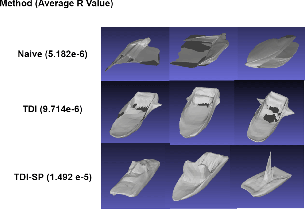
(H4) Average mean Hausdorff distance across the three trials between point clouds in training data set  $\mathbf{T}$ and point clouds of final generation of each method $\mathbf{P}$. Both percentage improvement and $p$-values are calculated with respect to the naïve method.
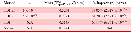
Finally, we visualize the designs in Figure 17 to gain some intuition about how these findings manifest. We observe that the naïve method tends to generate flat objects that do not look like human-designed watercraft. Thus aspects of watercraft that are not directly related to reducing the coefficient of drag are completely lost, which is usually not the goal of early conceptual design. Additionally, although we can see why the diversity is higher in terms of distance as not all objects are the same geometrically, the designs are conceptually nearly identical. In contrast, the TDI is able to successfully generate designs that resemble a human design; however, we are able to see how it fails to generate diversity in that all three randomly sampled designs appear to be the same. Finally, we observe how the proposed method is able to both capture the training data set and generate a diverse set of designs.
Also of note is the darker shaded regions of the meshes pictured for the aforementioned benchmarks. This is due to the mesh being ‘unclean’ with either surfaces with inverted normal vectors or surfaces that pierce the object. This finding is consistent with an observation made by Zhang et al. (Reference Zhang, Yang, Jiang, Nigam, Soji, Furuhata, Shimada and Kara2019) that when these are not constrained to interpolation between designs in the training set, they tend to produce invalid meshes. However, the TDI-SP-LSO avoids these defects in the meshes completely by producing designs that are not as distant from the training data without imposing a strict linear interpolation restriction.
Comparison of case study results
Combining insights from these experiments, we found in both cases that the proposed method was able to significantly improve the average performance of designs in the solution set relative to the training set, and we are thus unable to reject H1.
As for H2, we found in the ellipsoid test case that the proposed method produced more diverse designs, both in terms of the Hausdorff distance and visualization of designs in the 2D performance space. However, in the watercraft test case, we found that the average Hausdorff distance between designs produced by the naïve method was greater than that from the proposed method, contradicting both the previous experiment and H2. For this reason, we must reject H2 due to its formulation in terms of the Hausdorff distance. We believe this speaks to the limitations of simple objective diversity metrics to capture complex notions of diversity in design concepts. As Figure 17 shows, although the designs in the top row generated by the naïve method are more diverse in terms of the Hausdorff distance than those in the rows below it, they are not conceptually diverse.
H3 was similar to H2, but predicted improved diversity over the TDI method instead of the naïve method. In both the ellipsoid and watercraft test cases, this was confirmed by the Hausdorff distance, and in the ellipsoid case visually by the distribution of solution sets in the 2D performance space. Thus, we cannot reject H3.
H4 predicted that the proposed method would result in designs that are more similar to human-created designs in the data set in terms of the Hausdorff distance. The watercraft case study supported this prediction, as all TDI methods had a significantly lesser average distance to designs in the training set compared to the naïve approach. However, the ellipsoid test case contradicted this finding, as the naïve approach had the highest similarity to the training set in terms of the Hausdorff distance. Thus, we must reject H4. However, by once again examining visualizations of the generated objects in Figure 14, we see that a likely explanation for this contradiction is the case of ellipsoids that are rotated compared to designs in the training set. This indicates a possible need for a post-processing step, which normalized output designs in terms of their rotation.
6 Conclusion
We introduced a new method for GA-LSO that exploits the particular structure of the encoded latent vectors of point cloud GNNs to extract high performing designs from the latent space while maintaining both the knowledge captured by the training set and the diversity of generated designs. We demonstrated these aspects of the proposed method through a test case of a GNN trained to generate watercraft models, by framing an optimization task of identifying designs in the latent space with a low coefficient of drag. Moreover, our method relaxes several very simplifying assumptions employed in previous works related to the data format, performance metric, and optimization strategy.
This method has potential to be used as a tool for early conceptual design to aid the creative process in an organic way that supports emergence from previous generations of designs, while taking into account the desired performance metrics at this early stage. However, based on our work it is still unclear whether sparsity in the latent vectors can be exploited with GNNs of other data formats such as voxels or SDG. This is an area that requires further study.
Other possible extensions of this work include optimization methods that do not treat the generator as a black box and improve performance after training is complete, but instead cycle between data-based training updates and performance-based training updates. Extension to multi-objective optimization is another area of research that should be explored.
Acknowledgments
The authors would like to acknowledge Sean Lacey and Simon Miller for their contributions to this work.
Financial support
This research is funded in part by DARPA HR0011-18-2-0008. Any opinions, findings, or conclusions found in this paper are those of the authors and do not necessarily reflect the views of the sponsors.


 Open access