


1. Introduction
The shock-wave/laminar boundary-layer interaction is a fundamental problem of fluid mechanics and is of practical importance in the aerodynamics and propulsion of high-speed flight vehicles (Babinsky & Harvey Reference Babinsky and Harvey2011). If the adverse pressure gradient induced by the shock wave is large enough, the boundary layer separates from the wall and forms a separation bubble.
The shock-induced separated flow can support various local and global flow instabilities (Robinet Reference Robinet2007; Egorov, Neiland & Shvedchenko Reference Egorov, Neiland and Shvedchenko2011; Guiho, Alizard & Robinet Reference Guiho, Alizard and Robinet2016; Sansica, Sandham & Hu Reference Sansica, Sandham and Hu2016; Bugeat et al. Reference Bugeat, Robinet, Chassaing and Sagaut2022) that may lead to unsteadiness and a laminar‒turbulent transition. Experiments and direct numerical simulations (DNSs) with many canonical configurations (Chapman, Kuehn & Larson Reference Chapman, Kuehn and Larson1958; Ginoux Reference Ginoux1960; Simeonides & Haase Reference Simeonides and Haase1995; Benay et al. Reference Benay, Chanetz, Mangin and Vandomme2006; Willems, Gülhan & Steelant Reference Willems, Gülhan and Steelant2015; Roghelia et al. Reference Roghelia, Olivier, Egorov and Chuvakhov2017; Currao et al. Reference Currao, Choudhury, Gai, Neely and Buttsworth2020; Fu et al. Reference Fu, Karp, Bose, Moin and Urzay2021) have shown that strong interactions can promote the laminar‒turbulent transition near flow reattachment, which is frequently accompanied by streamwise streaks in the reattached boundary layer. These instabilities can also be understood by examining the spectrum of the linearised Navier‒Stokes operator. Due to the strong non-parallelism of the base flow, global stability analysis (GSA) is more relevant than local analysis. From a global stability point of view, a flow is called an oscillator if globally unstable and a noise amplifier if globally stable (Huerre & Monkewitz Reference Huerre and Monkewitz1990).
For shock impingement on a Mach 2.15 boundary layer, Robinet (Reference Robinet2007) found that the two-dimensional base flow becomes globally unstable to three-dimensional stationary disturbances beyond a critical incident shock angle by GSA. Similar observations were made in the hypersonic flow regime by Hildebrand et al. (Reference Hildebrand, Dwivedi, Nichols, Jovanović and Candler2018). For a Mach 5 double-wedge flow, Sidharth et al. (Reference Sidharth, Dwivedi, Candler, & Nichols and W2018) also found a stationary unstable mode beyond a critical deflection angle, which is in the form of streamwise streaks downstream of reattachment. A similar unstable mode was identified by Hao et al. (Reference Hao, Cao, Wen and Olivier2021) in a Mach 7.7 compression corner flow. Additional stationary and oscillatory modes appear as the ramp angle is further increased. A companion DNS study (Cao et al. Reference Cao, Hao, Klioutchnikov, Olivier and Wen2021) confirmed that global instability leads to a three-dimensional flow bifurcation to generate pairs of counterrotating streamwise vortices near flow reattachment. After the nonlinear saturation of the leading stationary mode, the flow exhibits broadband low-frequency unsteadiness. More recently, Cao et al. (Reference Cao, Hao, Klioutchnikov, Wen, Olivier and Heufer2022) observed the laminar‒turbulent transition through the breakdown of streamwise vortices by further increasing the Reynolds number. No upstream disturbances were added in the DNS. Under both flow conditions, the distributions of the surface pressure and heat flux, and the spanwise wavelengths of the streamwise streaks agree well with the experiments (Roghelia et al. Reference Roghelia, Olivier, Egorov and Chuvakhov2017). This suggests that the dynamics of a strong oscillator are dominated by its intrinsic instability.
In contrast to oscillators, noise amplifiers feed on the continuous input of external disturbances. Global resolvent analysis is an effective tool to study the dynamics of noise amplifiers, which considers the response of a globally stable flow to time-harmonic forcing with no assumption on the parallelism of the flow (Sipp & Marquet Reference Sipp and Marquet2013; Bugeat et al. Reference Bugeat, Chassaing, Robinet and Sagaut2019). The optimal response can be either modal resonance or non-modal pseudo-resonance due to the non-normality of the linearised Navier‒Stokes operator (Schmid Reference Schmid2007). The latter can be further divided into convective- and component-type non-normalities (Chomaz Reference Chomaz2005). If the base flow is weakly non-parallel, the convective-type non-normality is related to the ‘normal-mode’ instabilities obtained from local analysis, such as Mack's first and second modes (Mack Reference Mack1984), while the component-type non-normality may share some similarities with the algebraic instabilities (Ellingsen & Palm Reference Ellingsen and Palm1975) obtained from transient growth analysis (Hanifi, Schmid & Henningson Reference Hanifi, Schmid and Henningson1996; Tumin & Reshotko Reference Tumin and Reshotko2003; Tempelmann, Hanifi & Henningson Reference Tempelmann, Hanifi and Henningson2012; Quintanilha et al. Reference Quintanilha, Paredes, Hanifi and Theofilis2022). The dynamics of the shock-induced separated flow as a noise amplifier is further complicated by its non-parallelism and has attracted much attention.
Balakumar, Zhao & Atkins (Reference Balakumar, Zhao and Atkins2005) examined the evolution of small-amplitude second-mode disturbances over a 5.5° compression corner at Mach 5.373 by two-dimensional DNS. The disturbances grow exponentially upstream of separation and downstream of reattachment but remain neutral across the separation region. Similar findings were reported by Egorov et al. (Reference Egorov, Novikov and Fedorov2006). For the same flow conditions and geometry, Novikov, Egorov & Fedorov (Reference Novikov, Egorov and Fedorov2016) conducted DNS of a three-dimensional wave packet generated by a wall blowing suction pulse upstream of separation. Depending on the location of the pulse, the evolution of the wave packet is dominated by either the oblique first mode or the planar second mode. Sansica et al. (Reference Sansica, Sandham and Hu2016) numerically studied shock impingement on a Mach 1.5 boundary layer and triggered a laminar‒turbulent transition near flow reattachment by adding a pair of oblique first-mode waves determined by local analysis to the incoming boundary layer.
For a Mach 8 compression corner flow, Dwivedi et al. (Reference Dwivedi, Sidharth, Nichols, Candler and Jovanovic2019) found that the optimal response to forcing upstream of separation is in the form of steady streamwise streaks downstream of reattachment using resolvent analysis. It was also demonstrated that the baroclinic effects contribute most to the amplification of the streamwise vorticity perturbation. Lugrin et al. (Reference Lugrin, Beneddine, Leclercq, Garnier and Bur2021) conducted a high-fidelity simulation of a Mach 5 hollow-cylinder/flare flow with the inlet perturbed by white noise. The noise amplitude was chosen to reproduce the experimental length of the separation region (Benay et al. Reference Benay, Chanetz, Mangin and Vandomme2006). By performing spectral proper orthogonal decomposition and resolvent analysis, the transition process was shown to be associated with the breakdown of streamwise streaks near flow reattachment, which are generated through the nonlinear interaction of oblique first-mode waves upstream of separation and experience a linear amplification in the shear layer. More recently, Bugeat et al. (Reference Bugeat, Robinet, Chassaing and Sagaut2022) applied resolvent analysis to shock impingement on a Mach 2.15 boundary layer. For three-dimensional forcing, both modal resonance and non-modal pseudo-resonance were identified depending on the spanwise wavenumbers. The former represents a direct excitation of the leading global mode, while the latter corresponds to streamwise streaks.
A series of experiments (Esquieu et al. Reference Esquieu, Benitez, Schneider and Brazier2019; Benitez et al. Reference Benitez, Jewell, Schneider and Esquieu2020) was conducted with a cone–cylinder–flare geometry in a Mach 6 quiet wind tunnel at Purdue University. For a 10° flare large enough to induce flow separation, the surface pressure fluctuation measurements captured the second mode and a low-frequency instability on the flare. A similar low-frequency instability was found by Butler & Laurence (Reference Butler and Laurence2021) in the separated shear layer over a cone-flare model in a reflected shock tunnel at Mach 6 and was believed to be generated by the separation bubble. Paredes et al. (Reference Paredes, Scholten, Choudhari, Li, Benitez and Jewell2022) studied the linear evolution of the first and second modes from a location upstream of the cone–cylinder juncture to the end of the flare by solving the harmonic linearised Navier‒Stokes equations. Comparison with the experimental wall-pressure power spectra revealed that the low-frequency instability originates from the oblique first mode. However, they found that the axisymmetric laminar flow is globally unstable. In other words, the cone–cylinder–flare flow is a weak oscillator, which may influence the evolution of upstream disturbances after nonlinear saturation of the global mode (Li et al. Reference Li, Choudhari, Paredes and Scholten2022).
Despite these efforts, many questions regarding the response of shock-induced separated flow to upstream disturbances remain to be answered, e.g. the effect of the interaction strength, the competition between steady streamwise streaks and Mack's modes, the role of the global instability if the flow is marginally unstable, etc. To gain a deeper understanding of the dynamics of shock-induced separated flow as a noise amplifier, the present study investigates hypersonic laminar flow over a compression corner using a combination of computational fluid dynamics and global resolvent analysis, and determines the optimal responses and forcings over a range of flow conditions and geometries.
2. Geometric configuration and flow conditions
The experimental model tested in the hypersonic Aachen Shock Tunnel TH2 by Roghelia et al. (Reference Roghelia, Olivier, Egorov and Chuvakhov2017) is considered here, which has a flat plate of length L = 100 mm with a sharp leading edge (see figure 1). The length of the ramp is set to 100 mm. A Cartesian coordinate system is constructed with the origin at the leading edge, the x direction along the flat plate, the y direction perpendicular to the flat plate and the z direction satisfying the right-hand rule. A body-oriented coordinate system is also defined, where ξ is the distance along the model surface measured from the leading edge and η is the wall-normal distance from the model surface.

Figure 1. Computational domain and schematic of the compression corner configuration.
The baseline free-stream conditions are given as follows: M ∞ = 7.7, ρ ∞ = 0.021 kg m−3, T ∞ = 125 K and Re ∞ = 4.2 × 10⁶ m−1. The wall temperature is assumed to be room temperature (Tw = 293 K or Tw/T ∞ = 2.344) due to the short test time. Four ramp angles (α = 0°, 4°, 8° and 12°) are considered to achieve different interaction strengths. Note that α = 0° represents a hypersonic flat-plate boundary layer as a reference.
3. Computational details
3.1. Governing equations
The three-dimensional compressible Navier–Stokes equations are given in the following conservation form:
 \begin{equation}\frac{{\partial \boldsymbol{U}}}{{\partial t}} + \frac{{\partial \boldsymbol{F}}}{{\partial x}} + \frac{{\partial \boldsymbol{G}}}{{\partial y}} + \frac{{\partial \boldsymbol{H}}}{{\partial z}} = 0,\end{equation}
where U = (ρ, ρu, ρv, ρw, ρe)T is the vector of conservative variables and F, G and H are the vectors of fluxes. In these expressions, ρ is the density, u, v and w are the flow velocities in the x, y and z directions, and e is the total energy per unit mass. A calorically perfect Newtonian fluid is assumed to have a constant specific heat ratio of 1.4. Sutherland's law is used to calculate the dynamic viscosity. The thermal conductivity is obtained with a constant Prandtl number of 0.72. The flow-field variables are non-dimensionalised using the free-stream parameters and the length of the flat plate L.
It is assumed that the vector U can be decomposed into a two-dimensional steady base flow and a small-amplitude three-dimensional time-dependent perturbation as
 \begin{equation}\boldsymbol{U}(x,y,z,t) = \bar{\boldsymbol{U}}(x,y) + {\boldsymbol{U}^{\prime}}(x,y,z,t).\end{equation}
Hereafter, the overbar and prime represent base-flow and perturbation variables, respectively. Note that the base flow also satisfies (3.1). Substituting (3.2) into (3.1) and neglecting the higher-order terms leads to the governing equations of the perturbation as
 \begin{equation}\frac{{\partial {\boldsymbol{U}^{\prime}}}}{{\partial t}} + \frac{{\partial {\boldsymbol{F}^{\prime}}}}{{\partial x}} + \frac{{\partial {\boldsymbol{G}^{\prime}}}}{{\partial y}} + \frac{{\partial {\boldsymbol{H}^{\prime}}}}{{\partial z}} = 0.\end{equation}
3.2. Base-flow solver
The base-flow solutions are obtained using an in-house multiblock parallel finite-volume solver called PHAROS (Hao, Wang & Lee Reference Hao, Wang and Lee2016; Hao & Wen Reference Hao and Wen2020). The inviscid fluxes are calculated using the modified Steger–Warming scheme (MacCormack Reference Maccormack2014), while the viscous fluxes are computed with the second-order central difference. An implicit line relaxation method (Wright, Candler & Bose Reference Wright, Candler and Bose1998) is employed for pseudo time stepping, which allows a Courant–Friedrichs–Lewy number up to 103. The free-stream conditions are specified on the left and upper boundaries of the computational domain (see figure 1). A simple extrapolation is used on the right boundary. The no-slip condition is applied to the isothermal model surface. The grid independence of the base-flow simulations is verified in Appendix A. Subsequent stability analysis requires a clean base flow with little numerical noise. For all cases, a ten orders of magnitude reduction in the Euclidean norm of the density residual is achieved (see Appendix A).
3.3. Resolvent analysis
The operator form of (3.3) is given by
 \begin{equation}\frac{{\partial {\boldsymbol{U}^{\prime}}}}{{\partial t}} = {\boldsymbol{\mathsf{A}}\boldsymbol{U}^{\prime}},\end{equation}
where  $\boldsymbol{\mathsf{A}}$ is the Jacobian matrix evaluated using the base flow. The perturbation U′ is assumed to be in the following modal form:
 \begin{equation}{\boldsymbol{U}^{\prime}}(x,y,z,t) = \hat{\boldsymbol{U}}(x,y)\exp [\textrm{i}\beta z - \textrm{i}({\omega _r} + \textrm{i}{\omega _i})t],\end{equation}
where  $\hat{\boldsymbol{U}}$ is the two-dimensional eigenfunction, β is the spanwise wavenumber, ωr is the angular frequency and ωi is the growth rate. Substituting (3.5) into (3.4) leads to an eigenvalue problem as
 \begin{equation}- ({\omega _r} + \textrm{i}{\omega _i})\hat{\boldsymbol{U}} = \boldsymbol{\mathsf{A}}\hat{\boldsymbol{U}},\end{equation}
which is also discretised using the finite-volume method in accordance with the base-flow solver. The inviscid fluxes are calculated using the modified Steger–Warming scheme near discontinuities and a central scheme in smooth regions. The viscous fluxes are computed with the second-order central difference. The boundary conditions are consistent with those for the base flow. Sponge layers are placed near the far-field and outflow boundaries to ensure no reflection of perturbations (Mani Reference Mani2012). More details regarding the numerical settings can be found in our previous work (Reference Hao, Cao, Wen and OlivierHao et al. 2021).
The discretised eigenvalue problem is solved using the implicitly restarted Arnoldi method implemented in ARPACK (Sorensen et al. Reference Sorensen, Lehoucq, Yang and Maschhoff1996) for a given β in the shift-invert mode. The inversion step is achieved using the lower‒upper decomposition implemented in SuperLU (Li et al. Reference Li, Demmel, Gilbert, Grigori, Shao and Yamazaki1999). For each shift, 100 eigenvalues are requested with a Krylov subspace of size 250. All the eigenvalues are converged with  ${\parallel} \boldsymbol{\mathsf{A}}\hat{\boldsymbol{U}} + ({\omega _r} + \textrm{i}{\omega _i})\hat{\boldsymbol{U}}\parallel{/}(\omega _r^2 + \omega _r^2) \le {10^{ - 10}}$. The flow is globally unstable if an eigenvalue with ωi > 0 can be found. Our previous study showed that the compression corner flow at the baseline flow conditions is globally unstable when the ramp angle is greater than or equal to 13° (Hao et al. Reference Hao, Cao, Wen and Olivier2021).
In this study, only globally stable flows are considered. In other words, all initial perturbations decay to zero in the case of no external forcing. To study the behaviour of the flow as a noise amplifier, a small-amplitude forcing term is added to (3.4) as
 \begin{equation}\frac{{\partial {\boldsymbol{U}^{\prime}}}}{{\partial t}} = \boldsymbol{\mathsf{A}}\boldsymbol{U^{\prime}} + {\boldsymbol{\mathsf{B}}\boldsymbol{f}^{\prime}},\end{equation}
where matrix  $\boldsymbol{\mathsf{B}}$ constrains the forcing to a localised region. If the forcing is assumed to be harmonic in time and in the spanwise direction as
 \begin{equation}{\boldsymbol{f}^{\prime}}(x,y,z,t) = \hat{\boldsymbol{f}}(x,y)\,\textrm{exp}(\textrm{i}\beta z - \textrm{i}{\omega _r}t),\end{equation}
the long-time solution of (3.7) takes the same form as
 \begin{equation}{\boldsymbol{U}^{\prime}}(x,y,z,t) = \hat{\boldsymbol{U}}(x,y)\,\textrm{exp}(\textrm{i}\beta z - \textrm{i}{\omega _r}t).\end{equation}
One should distinguish (3.9) from (3.5) as they have different physical interpretations. Substituting (3.8) and (3.9) into (3.7) gives
 \begin{equation}\hat{\boldsymbol{U}} = \boldsymbol{\mathsf{RB}}\hat{\boldsymbol{f}},\quad \boldsymbol{\mathsf{R}} = {( - {\omega _r}\boldsymbol{\mathsf{I}} - \boldsymbol{\mathsf{A}})^{ - 1}},\end{equation}
which represents the relationship between the forcing and its linear response (Bugeat et al. Reference Bugeat, Chassaing, Robinet and Sagaut2019). Here, matrix  $\boldsymbol{\mathsf{R}}$ is the resolvent matrix and matrix $\boldsymbol{\mathsf{I}}$ is the identity matrix. We are interested in finding the forcing and response that maximise the energy amplification (often referred to as the gain). In this study, the optimal gain σ is defined by
 \begin{equation}{\sigma ^2}(\beta ,{\omega _r}) = \mathop {\max }\limits_{\hat{\boldsymbol{f}}} \frac{{\parallel \hat{\boldsymbol{U}}{\parallel _E}}}{{\parallel \boldsymbol{\mathsf{B}}\hat{\boldsymbol{f}}{\parallel _E}}}.\end{equation}
The Chu energy (Chu Reference Chu1965) is used to evaluate the energy norm as
 \begin{equation}\parallel \hat{\boldsymbol{U}}{\parallel _E} = {\hat{\boldsymbol{U}}^ \ast }{\boldsymbol{\mathsf{M}}\hat{\boldsymbol{U}}},\end{equation}
where the superscript * denotes the complex conjugate and  $\boldsymbol{\mathsf{M}}$ is the weight matrix. The expression of matrix $\boldsymbol{\mathsf{M}}$ is given by Bugeat et al. (Reference Bugeat, Chassaing, Robinet and Sagaut2019). As demonstrated by Sipp & Marquet (Reference Sipp and Marquet2013), Bugeat et al. (Reference Bugeat, Chassaing, Robinet and Sagaut2019) and Dwivedi et al. (Reference Dwivedi, Sidharth, Nichols, Candler and Jovanovic2019), the optimisation problem (3.11) can be converted to an eigenvalue problem as
 \begin{equation}{\boldsymbol{\mathsf{B}}^ \ast }{{\boldsymbol{\mathsf{M}}}^{ - 1}}{\boldsymbol{\mathsf{R}}^ \ast }{\boldsymbol{\mathsf{MRB}}\hat{\boldsymbol{f}}} = {\sigma ^2}\hat{\boldsymbol{f}},\end{equation}
which is solved using ARPACK for a given β and ωr in the regular mode. Five eigenvalues are requested with a Krylov subspace of size 12. All the eigenvalues are converged with the same relative residuals as in the GSA. During this process, the inverses of  $\boldsymbol{\mathsf{R}}$ and its conjugate transpose are calculated using SuperLU. The largest eigenvalue represents the optimal gain, and the corresponding eigenfunction represents the optimal forcing. The optimal response can be readily obtained via (3.10). The grid independence of the resolvent analysis is verified in Appendix A, and the current resolvent analysis solver is validated in Appendix B.
The resolvent analysis and the temporal transient growth analysis describe the response of the flow to external forcing and initial conditions, respectively (Schmid Reference Schmid2007). If the forcing and response are constrained at two different streamwise locations, the resolvent analysis is equivalent to the spatial transient growth analysis (Tumin & Reshotko Reference Tumin and Reshotko2003). In this study, the forcing is always localised at xf/L = 0.2 to represent upstream disturbances, which can be introduced through the receptivity of free-stream noise, leading-edge imperfection, surface roughness, etc. In this case, the submatrices of matrix  $\boldsymbol{\mathsf{B}}$ are set to the identity matrix in cells at the forcing location and zero elsewhere. In contrast, the response in the entire computational domain is considered. In fact, the optimal response is insensitive to the forcing location (see Appendix C).
4. Results
4.1. Base flows and stability analysis
We first examine the general features of the base flows with different ramp angles. According to the classical triple-deck theory (Neiland Reference Neiland1969; Stewartson & Williams Reference Stewartson and Williams1969), supersonic flow over a compression corner is governed by a scaled ramp angle defined as
 \begin{equation}{\alpha ^ \ast } = \frac{{{Re}_L^{1/4}\alpha }}{{{C^{1/4}}{\lambda ^{1/2}}{{(M_\infty ^2 - 1)}^{1/4}}}},\end{equation}
where α is in radians, C is the Chapman–Rubesin parameter and λ equals 0.332 in a Blasius boundary layer. Previous studies have shown that incipient separation occurs when α* ≈ 1.57 (Rizzetta, Burggraf & Jenson Reference Rizzetta, Burggraf and Jenson1978; Ruban Reference Ruban1978; Cassel, Ruban & Walker Reference Cassel, Ruban and Walker1995), and secondary separation forms beneath the primary bubble when α* is between 3 and 5 (Smith & Khorrami Reference Smith and Khorrami1991; Korolev, Gajjar & Ruban Reference Korolev, Gajjar and Ruban2002; Shvedchenko Reference Shvedchenko2009; Gai & Khraibut Reference Gai and Khraibut2019). The precise critical values depend on the wall-to-total temperature ratio (Egorov et al. Reference Egorov, Neiland and Shvedchenko2011; Hao et al. Reference Hao, Cao, Wen and Olivier2021). For the baseline flow conditions considered in this study, α = 0°, 4°, 8° and 12° correspond to α* = 0, 1.147, 2.295 and 3.442, respectively. Therefore, flow separation is expected for the two larger ramp angles.
Figure 2 shows the distributions of the skin friction coefficient Cf, surface Stanton number St and surface pressure coefficient Cp for different ramp angles. The surface quantities Cf, St and Cp are defined by
 \begin{equation}{C_f} = \frac{{{\tau _w}}}{{0.5{\rho _\infty }u_\infty ^2}},\quad St = \frac{{{q_w}}}{{0.5{\rho _\infty }u_\infty ^3}},\quad {C_p} = \frac{{{p_w}}}{{0.5{\rho _\infty }u_\infty ^2}},\end{equation}
where τw, qw and pw are the surface shear stress, heat flux and pressure, respectively. Also shown in the figure is the distribution of the surface pressure gradient dCp/ds*, where s* is the non-dimensional distance along the model surface measured from the leading edge. When α > 0°, an oblique shock is induced by the flow deflection, which elevates the pressure on the ramp and poses an adverse pressure gradient on the boundary layer. At α = 4°, the pressure gradient peaks at the corner, which is not strong enough to cause flow separation. In response, Cf suddenly drops near the corner and slowly rises on the ramp. The St behaves in a similar way to Cf. As α is increased to 8°, the minimum Cf has crossed zero to form the separation and reattachment points marked by the open circles. Meanwhile, the pressure gradient exhibits two local maxima separated by a local minimum. At α = 12°, the local minimum becomes negative and thus poses an adverse pressure gradient to the reverse flow boundary layer. The deceleration of the reverse flow generates a local maximum of Cf near the corner, as reported by Smith & Khorrami (Reference Smith and Khorrami1991), Korolev et al. (Reference Korolev, Gajjar and Ruban2002) and Gai & Khraibut (Reference Gai and Khraibut2019). The local maximum of Cf is still negative, which indicates that the flow is prior to secondary separation. The presence of a pressure plateau region connecting the separation and reattachment processes is indicative of large separation (Burggraf Reference Burggraf1975). The small fluctuations of the surface quantities near x/L = 1.6 are caused by the impingement of an expansion wave induced by the interaction of the separation and reattachment shock waves.

Figure 2. Distributions of the (a) skin friction coefficient, (b) surface Stanton number, (c) surface pressure coefficient and (d) surface non-dimensional pressure gradient for different ramp angles. Open circles, separation and reattachment points; horizontal line, zero skin friction; vertical line, corner.
It is well known that flow separation can support self-sustained instability (Theofilis Reference Theofilis2011). For hypersonic flow over a compression corner, our previous study (Hao et al. Reference Hao, Cao, Wen and Olivier2021) demonstrated that the leading global instability is a three-dimensional stationary mode, which becomes unstable beyond a critical scaled ramp angle. For the current flow conditions, the critical value of α* is approximately 3.729 (α = 13°). Although the base flows at the four ramp angles are globally stable, modal resonance may be important when the spanwise wavenumber and frequency of the forcing are close to those of the leading mode. Figure 3(a) presents the growth rate of the least stable mode as a function of spanwise wavenumber for the α = 12° case. The growth rate peaks at βL = 48.0 (λ/L = 0.130) with the corresponding eigenvalue spectrum shown in figure 3(b). There is another stationary mode beneath the leading mode. These two modes move towards each other as β is increased and eventually meet to form a pair of conjugate oscillatory modes. As demonstrated by Hao et al. (Reference Hao, Cao, Wen and Olivier2021), modal coalescence generates a dominant small-wavelength mode as the flow is further destabilised. The eigenfunction of the least stable mode at βL = 48.0 is visualised in figure 4. The perturbation u′ is present in both the separation region and the reattached boundary layer, whereas w′ is mainly confined to the separation bubble with an opposite sign in the upstream and downstream regions. Such features have been observed by Sidharth et al. (Reference Sidharth, Dwivedi, Candler, & Nichols and W2018) for hypersonic flow over a slender double wedge and by Boin et al. (Reference Boin, Robinet, Corre and Deniau2006), Robinet (Reference Robinet2007) and Hildebrand et al. (Reference Hildebrand, Dwivedi, Nichols, Jovanović and Candler2018) for shock impingement on a flat plate. The leading mode also resembles the self-excited stationary mode found in an incompressible separation bubble (Theofilis et al. Reference Theofilis, Hein and Dallmann2000). In addition, there are no evident perturbations in the inviscid region behind the separation shock in contrast to the global modes found by Hao et al. (Reference Hao, Fan, Cao and Wen2022) over a 25°−55° double cone and by Sawant, Theofilis & Levin (Reference Sawant, Theofilis and Levin2022) over a 30°−55° double wedge. This is because the current shock interaction is much weaker than their cases.

Figure 3. (a) Growth rate of the least stable global mode as a function of spanwise wavenumber and (b) eigenvalue spectrum at βL = 48.0 (λ/L = 0.130) at α = 12°. Horizontal line, zero growth rate.

Figure 4. Real parts of (a) streamwise velocity perturbation u′ and (b) spanwise velocity perturbation w′ of the least stable global mode at βL = 48.0 (λ/L = 0.130) for the α = 12° case. The contour levels are evenly spaced between ±0.25 of the maximum absolute values. Black lines, dividing streamline and solid wall; open circles, separation and reattachment points.
In addition to the global stability of the base flows, the incoming and reattached boundary layers may support convectively unstable Mack's first and second modes. The wall-normal profile of the base flow is extracted at x/L = 0.5. Note that the profile is the same for different ramp angles, as the location is upstream of separation. Further assuming that the perturbation is harmonic in the streamwise direction allows the application of a local ‘normal-mode’ analysis. In this analysis, the flow is assumed to be parallel in the ξ direction. The spatial stability problem is solved by a Chebyshev pseudo-spectral method to obtain the global eigenvalue spectrum and an iterative fourth-order compact finite difference scheme to increase the accuracy of solutions without interpolating the base flow (see Guo et al. Reference Guo, Gao, Jiang and Lee2020 for more details). Figure 5 shows the contour of the streamwise growth rate in the β‒ωr space with the neutral curve highlighted in black. As expected, the Mach 7.7 flat-plate boundary layer with a cold wall only supports Mack's second mode, which is most amplified as a planar wave at ωrL/u ∞ = 110 ( f = 305.5 kHz). The three-dimensional second mode spreads to βL = 133.4 (λ/L = 0.047).

Figure 5. Contour of streamwise growth rate in the space of spanwise wavenumber and angular frequency at x/L = 0.5 obtained from the local stability analysis. Black line, neutral curve.
Wall-normal distributions of the streamwise velocity us and temperature T are then extracted at the midpoint of the ramp (ξ/L = 1.5) and compared in figure 6 as a function of distance from the wall yn for different ramp angles. The velocity and temperature at the edge of the boundary layer vary according to inviscid theory of oblique shock waves. As α is increased, the boundary-layer thickness decreases, and the temperature peak increases. Local stability analysis is performed using these profiles to obtain the stability diagrams, as shown in figure 7. Again, there is no first mode. From α = 0° to 12°, the second mode is destabilised at higher peak frequencies, which is consistent with the variation in the boundary-layer thickness. Meanwhile, the unstable region extends to higher spanwise wavenumbers. As seen later, the overlap between the second-mode frequencies in the incoming and reattached boundary layers for the α = 4° case allows a continuous excitation of the disturbances.

Figure 6. Wall-normal distributions of (a) streamwise velocity and (b) temperature at the midpoint of the ramp (ξ/L = 1.5) for different ramp angles.

Figure 7. Contours of streamwise growth rate in the space of spanwise wavenumber and angular frequency at the midpoint of the ramp (ξ/L = 1.5) at (a) α = 0°, (b) α = 4°, (c) α = 8° and (d) α = 12°. Black line, neutral curve.
4.2. Optimal disturbances
Global resolvent analysis is performed over a wide range of spanwise wavenumbers and angular frequencies using the base-flow solutions. Note that the forcing is localised at xf/L = 0.2. The resulting optimal gain is plotted in the β‒ωr space in figure 8 for different ramp angles. For the flat-plate case, the maximum gain is achieved near βL = 96.3 (λ/L = 0.065) as the frequency approaches zero. The optimal gain is almost independent of the frequency for ωrL/u ∞ ≤ 1 ( f ≤ 2.8 kHz). As seen later, the low-frequency response is in the form of streamwise streaks, which have been extensively identified by temporal and spatial analyses of transient growth in both incompressible and compressible boundary layers (Hanifi et al. Reference Hanifi, Schmid and Henningson1996; Andersson et al. Reference Andersson, Berggren and Henningson1999; Tumin & Reshotko Reference Tumin and Reshotko2003; Tempelmann et al. Reference Tempelmann, Hanifi and Henningson2012). Another local maximum of the optimal gain (approximately 1/4 of the global maximum) can be found on the axis of βL = 0 at ωrL/u ∞ ≈ 75 ( f ≈ 208.3 kHz). The high-frequency response is related to Mack's second mode. Note that the gain of the second mode may exceed that of the streamwise streaks for a longer flat plate. In the framework of resolvent analysis, the streamwise streaks and the second-mode waves represent the component- and convective-type non-normalities, respectively. Similar observations were made by Bugeat et al. (Reference Bugeat, Chassaing, Robinet and Sagaut2019) for a Mach 4.5 flat-plate boundary layer except that they found a third local maximum gain corresponding to Mack's first mode. As predicted by the local analysis, the current flow conditions support no first mode.

Figure 8. Contours of optimal gain in the space of spanwise wavenumber and angular frequency at (a) α = 0°, (b) α = 4°, (c) α = 8° and (d) α = 12°.
At α = 4°, the contour of the optimal gain is similar to that for the flat plate. The low-frequency peak is further amplified and shifts to a higher wavenumber (βL = 160.1 or λ/L = 0.039). The second mode is also enhanced and moves towards a higher frequency (ωrL/u ∞ ≈ 102 or f ≈ 277.7 kHz); however, its gain is still less than that of the streamwise streaks. As α is further increased, the maximum optimal gain of the streamwise streaks and the corresponding wavenumber continue to grow. In contrast, the second-mode peak is separated into two local maxima. One is almost fixed at ωrL/u ∞ = 102, and the other has a similar frequency to the most amplified mode predicted by the local stability analysis on the ramp (see figure 7).
To closely examine the dependence of the optimal gain on the spanwise wavenumber for the streamwise streaks and the second mode, slices at two representative frequencies (ωrL/u ∞ = 10−1 and 102) are extracted from the optimal-gain contours, as shown in figure 9. At the lower frequency, increasing the ramp angle elevates the optimal gain over the considered range of wavenumbers. The preferential wavenumbers at α = 0°, 4°, 8° and 12° are βL = 96.3, 160.1, 206.8 and 252.7 (λ/L = 0.065, 0.039, 0.030 and 0.025), respectively. At the higher frequency, two local maxima can be observed for each ramp angle. The two-dimensional peak is associated with the second mode. As described earlier, the second mode is first promoted and then stabilised as α is increased. The three-dimensional peak is the unsteady counterpart of the steady streamwise streaks.
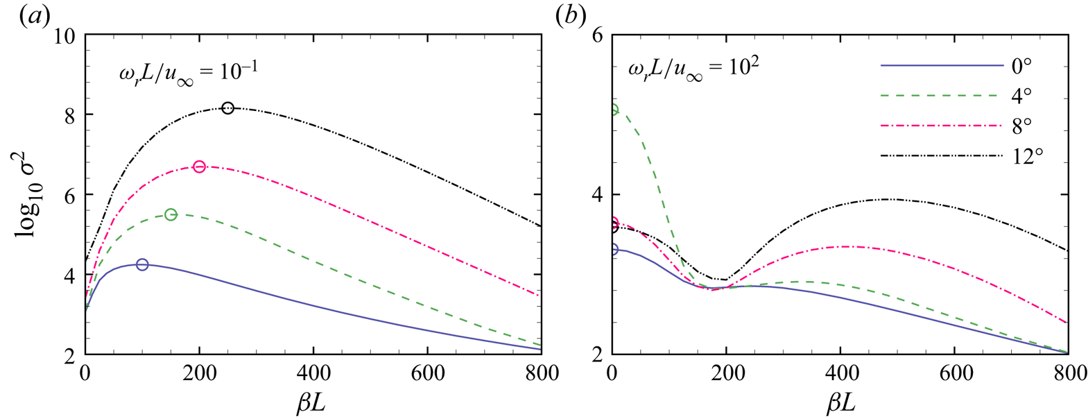
Figure 9. Optimal gains at (a) ωrL/u ∞ = 10−1 and (b) ωrL/u ∞ = 102 as a function of spanwise wavenumber for different ramp angles. Open circles, local maxima of interest.
The optimal responses and forcings of the most amplified streamwise streaks (denoted by the open circles in figure 9a) are presented in figure 10. For the flat plate, the forcing is in the form of streamwise vortices with most of the kinetic energy in the wall-normal and spanwise velocity components. The flow response is streamwise streaks with the kinetic energy contributed mostly by the streamwise velocity perturbation, i.e.  $|u\prime |\gg |v\prime |$ and $|u\prime |\gg |w\prime |$ (not shown here). Such a component-wise energy transfer is usually attributed to the lift-up mechanism (Landahl Reference Landahl1980). Interestingly, the forcing stretches out of the boundary layer to the free stream. For the compression corners, the optimal responses resemble the flat-plate result and experience a strong amplification in the interaction region. The optimal forcings are also streamwise vortices; however, the contribution from the wall-normal velocity perturbation becomes more important for larger ramp angles. In particular, the streamwise streaks are convected downstream above the dividing streamline with no evident interaction with the separation bubble at α = 12°. Only weak perturbations can be seen inside the separation bubble near the reattachment point, indicative of insignificant modal resonance. A similar steady optimal response over a compression corner was obtained by Dwivedi et al. (Reference Dwivedi, Sidharth, Nichols, Candler and Jovanovic2019) under one of the experimental conditions of Chuvakhov et al. (Reference Chuvakhov, Borovoy, Egorov, Radchenko, Olivier and Roghelia2017). However, they found a significant contribution to the amplification of the streamwise streaks from the separation bubble, in contrast to the present study. In fact, our GSA shows that their flow conditions are weakly unstable to three-dimensional perturbations, which invalidates the assumption of resolvent analysis. The interplay between the intrinsic instability and upstream disturbances was addressed in a companion study (Cao et al. Reference Cao, Hao, Guo, Wen and Klioutchnikov2023).

Figure 10. Optimal responses (left) and forcings (right) associated with the most amplified streamwise streaks at (a) α = 0°, (b) α = 4°, (c) α = 8° and (d) α = 12°. Open circles, separation and reattachment points; black dashed lines, the edge of the boundary layer at xf/L = 0.2.
The temperature components of the optimal responses are shown in figure 11 for different ramp angles. As expected, they also take the form of streaks with alternating high and low temperature in the spanwise direction (Tempelmann et al. Reference Tempelmann, Hanifi and Henningson2012). The temperature perturbation is concentrated near the edge of the boundary layer for the flat plate but extends to the near-wall region for the compression corners (explained in § 4.3). Although the amplitude of the temperature perturbation is larger than that of the streamwise velocity perturbation (see figure 10), the overall Chu energy of the response is mainly contributed by the kinetic energy. The density components of the optimal responses can be found in Appendix D.

Figure 11. Temperature components of the optimal responses associated with the most amplified streamwise streaks at (a) α = 0°, (b) α = 4°, (c) α = 8° and (d) α = 12°. Open circles, separation and reattachment points.
To quantitatively describe the spatial evolution of the optimal responses, the Chu energy density of the most amplified streamwise streaks is integrated in the wall-normal direction along the model surface, as shown in figure 12. Note that the Chu energy of the response is normalised by that of the forcing, which allows a direct comparison between different cases. For the compression corners, the flat-plate results at the same spanwise wavenumbers are also plotted. It is confirmed that the streamwise streaks originate from the transient growth of streamwise vortices on the flat plate with a preferential spanwise wavelength and experience a strong amplification in the interaction region until reaching the maximum energy at the end of the ramp. For the large-separation case (α = 12°), the amplification seems to be associated with the separation and reattachment processes while remaining moderate in the pressure plateau region (see figure 2c). It is indicated that the most amplified streamwise streaks are in essence non-modal pseudo-resonance. As explained later, the amplification across the interaction region is mainly due to the Görtler instability. The streamline curvature is high near the separation and reattachment points and low along the shear layer, resulting in two separate stages of energy growth. Also shown in figure 12(d) is the Chu energy density integrated above the dividing streamline represented by the red dashed line. It is confirmed that the separation bubble contributes little to the optimal response. The N factor can be defined by the natural logarithm of the ratio between the maximum Chu energy and the value at the forcing location multiplied by a factor of 1/2. The N factors of the most amplified streamwise streaks at α = 0°, 4°, 8° and 12° are 3.42, 5.76, 7.35 and 9.13, respectively.

Figure 12. Distributions of Chu energy density integrated in the wall-normal direction associated with the most amplified streamwise streaks at (a) α = 0°, (b) α = 4°, (c) α = 8° and (d) α = 12°. Vertical lines, separation and reattachment points; dash–dotted lines, flat-plate results. Red dashed line, the Chu energy density integrated above the dividing streamline for the α = 12° case.
Modal resonance may be important when the forcing wavenumber and frequency are close to those of the least stable global mode. Figure 13 presents the real part of the spanwise velocity perturbation at βL = 50.0 and ωrL/u ∞ = 10−1 for the α = 12° case. The perturbation structure resembles the global mode shown in figure 4(b) in the separation region, which indicates that the global mode is excited by the forcing and contributes to the overall growth of the response. The contribution can be clearly seen by comparing the wall-normal integrals of the Chu energy density for the modal and non-modal resonances (i.e. βL = 50.0 and 252.7) in figure 14. Nonetheless, the largest energy of the non-modal resonance achieved at the end of the ramp is two orders of magnitude greater than that of the modal resonance.

Figure 13. Real part of spanwise velocity perturbation w′ of the optimal response at βL = 50.0 and ωrL/u ∞ = 10−1 for the α = 12° case. The contour levels are evenly spaced between ±0.5 of the maximum absolute value. Open circles, separation and reattachment points.

Figure 14. Distributions of Chu energy density integrated in the wall-normal direction associated with the modal and non-modal resonances at ωrL/u ∞ = 10−1 for the α = 12° case. Dashed lines, separation and reattachment points.
It is also of interest to examine the optimal responses associated with the second mode. Figures 15 and 16 show the pressure perturbation fields and the corresponding Chu energy densities integrated in the wall-normal direction at βL = 0 and ωrL/u ∞ = 102 (denoted by the open circles in figure 9b). Also shown in figure 14 are two line segments, whose slopes are determined from the spatial growth rates predicted by the local stability analysis with the same β and ωr at ξ/L = 0.5 and 1.5 for the α = 4° case (see figures 5 and 7). The evolution of the perturbations exhibits a typical two-cell structure in the incoming boundary layer for different cases. Partly contributed by the component-type non-normality, the spatial growth rate is slightly larger than that predicted by the local analysis. For the flat plate, the second mode is amplified on the upstream half of the flat plate and attenuated in the downstream half. In contrast, the perturbations continue to grow on the ramp at α = 4° (see figure 16). The growth rate on the ramp agrees well with the local-analysis prediction, which indicates that the growth is mainly due to the convective-type non-normality. The N factor of the second mode is 4.84, which is comparable to that of the streamwise streaks. As α is further increased, the second mode remains neutral inside the separation region and oscillates along the ramp, which is consistent with the previous findings of Balakumar et al. (Reference Balakumar, Zhao and Atkins2005). Radiation of the second-mode energy along the oblique shocks can be seen, as reported by Butler & Laurence (Reference Butler and Laurence2021). Downstream of reattachment, the perturbations are stabilised with a non-monotonic evolution, and the two-cell structure no longer exists. For the large-separation case, a three-cell structure forms after the second mode enters the separation bubble, which was attributed to the excitation of an acoustic discrete mode (Egorov et al. Reference Egorov, Novikov and Fedorov2006). Other components of the optimal responses can be found in Appendix D.

Figure 15. Real parts of pressure perturbations associated with the two-dimensional second mode at ωrL/u ∞ = 102 for different ramp angles: (a) α = 0°; (b) α = 4°; (c) α = 8°; (d) α = 12°.

Figure 16. Distributions of Chu energy density integrated in the wall-normal direction associated with the two-dimensional second mode at ωrL/u ∞ = 102 for different ramp angles. The slopes of the short line segments are determined from the spatial growth rates of the most unstable mode predicted by the local stability analysis at ξ/L = 0.5 and 1.5 at βL = 0 and ωrL/u ∞ = 102 for the α = 4° case.
Additional second-mode peaks are examined at ωrL/u ∞ = 150 and 220 for the α = 8° and 12° cases, respectively. The corresponding pressure perturbation fields and the Chu energy densities integrated in the wall-normal direction are shown in figures 17 and 18. The perturbations decay significantly on the flat plate followed by a growth along the reattached boundary layer as predicted by the local stability analysis. Interestingly, the α = 8° case supports a continuous amplification of the second mode on the ramp similar to the α = 4° case, while the second mode starts to decay near the outlet at α = 12°. It is indicated that the reattached boundary-layer thickness grows slowly at moderate ramp angles. The N factors for these two cases are 4.20 and 3.74, which are much lower than those of the corresponding streamwise streaks. However, if only the ramp region is focused on, the N factors of the second mode and the streamwise streaks are comparable at α = 8°. In this case, the role of the second mode in the early stages of transition merits further investigation.

Figure 17. Real parts of pressure perturbations associated with the two-dimensional second mode for different ramp angles: (a) α = 8° at ωrL/u ∞ = 150; (b) α = 12° at ωrL/u ∞ = 220.

Figure 18. Distributions of Chu energy density integrated in the wall-normal direction associated with the two-dimensional second mode at ωrL/u ∞ = 150 for the α = 8° case and ωrL/u ∞ = 220 for the α = 12° case. The slopes of the short line segments are determined from the spatial growth rates predicted by the local stability analysis at ξ/L = 1.5.
4.3. Corner rounding
To further understand the physical mechanisms that amplify the streamwise streaks in the interaction region, the corner of the 12° ramp is rounded such that the circular arc is tangential to both the flat plate and ramp. Similar geometries have been used to experimentally and numerically study the Görtler instability induced by wall curvature (Floryan Reference Floryan1991; de Luca et al. Reference de Luca, Cardone, de la Chevalerie and Fonteneau1993; Saric Reference Saric1994; Chen, Huang & Lee Reference Chen, Huang and Lee2019). Two corner radii (rc/L = 1.9 and 3.8) are considered with the points of tangency on the flat plate xt/L = 0.8 and 0.6.
Figure 19 shows the distributions of Cf and Cp for different corner radii. Sufficient corner rounding alleviates the adverse pressure gradient and thus eliminates the separation region. Such a strategy can be used to stabilise the global instability of supersonic flow over a compression corner, which will be addressed in a future study. Global resolvent analysis is then performed using the base flows with corner rounding at ωrL/u ∞ = 10−1. As expected, the most amplified optimal responses and forcings are found to be streamwise streaks and vortices for rc/L = 1.9 and 3.8, respectively (see figure 20). Cossu et al. (Reference Cossu, Chomaz, Huerre and Costa2000) performed spatial transient growth analysis of an incompressible boundary layer over a concave curved wall and found an optimal response and forcing similar to the present results. For rc/L = 1.9 and 3.8, the most amplified optimal responses occur at βL = 262.3 and 287.5 (λ/L = 0.024 and 0.022), respectively. Surprisingly, the preferential spanwise wavelengths are insensitive to corner radii and close to the sharp-corner value (βL = 252.7 or λ/L = 0.025). This finding may suggest that the total turning angle is more important than the curvature of the wall for the Görtler instability (Floryan Reference Floryan1991), which will be addressed in a future study.

Figure 19. Distributions of the (a) skin friction coefficient and (b) surface pressure coefficient for different corner radii. Open circles, separation and reattachment points and points of tangency; horizontal line, zero skin friction; vertical line, corner.

Figure 20. Optimal responses and forcings associated with the most amplified streamwise streaks for (a) rc/L = 1.9 and (b) rc/L = 3.8. Open circles, points of tangency; black dashed lines, the edge of the boundary layer at xf/L = 0.2.
The streamlines passing through point (x/L, y/L) = (0.5, 0.01) close to the edge of the local boundary layer are extracted for the sharp- and rounded-corner cases with the distributions of the Chu energy density along the streamlines presented in figure 21. Also shown in this figure are the distributions of the streamline curvature. For the sharp-corner case, the peaks in the curvature are due to flow separation and reattachment, whereas the curvature is small in the shear layer and reattached boundary layer. The energy density increases significantly where the curvature is large. With corner rounding, the curvature is approximately constant at L/rc above the circular arc. The energy density experiences exponential growth over the circular arc and reaches a peak close to the sharp-corner value at the end of the ramp.

Figure 21. Distributions of Chu energy density along a streamline passing through point (x/L, y/L) = (0.5, 0.01) associated with the most amplified streamwise streaks for (a) sharp corner, (b) rc/L = 1.9 and (c) rc/L = 3.8 at α = 12°. Open circles, separation and reattachment points and points of tangency. The slopes of the short line segments are determined from the spatial growth rates of the most unstable Görtler mode predicted by the local stability analysis.
The striking similarity between these cases indicates that the growth of the streamwise streaks in the interaction region is mainly due to the Görtler instability. To support this argument, local stability analysis is performed using three wall-normal profiles, which are assumed to be parallel in the ξ direction. For the two cases with corning rounding, the profiles are extracted at ξ/L = 1. The wall curvature is used to evaluate the Lamé coefficients in curvilinear coordinates (see Ren & Fu Reference Ren and Fu2015 for detailed expressions of the linear operators). For the sharp-corner case, the wall-normal profile is extracted at the reattachment point, where the wall curvature is zero. A representative curvature is computed by averaging the streamline curvatures from the wall to the edge of the reattached shear layer. The resulting curvature is approximately 1.12. The flow near the separation point is not considered here due to the strong non-parallelism.
As expected, the local stability analysis captures stationary Görtler modes at the most unstable spanwise wavenumbers for different cases, whose spatial growth rates are converted to the slopes of the line segments in figure 21. The streamwise velocity and temperature perturbations from the resolvent analysis and local stability analysis are compared in figure 22. The temperature perturbation has a larger magnitude than the streamwise velocity perturbation, which is a typical behaviour of the Görtler instability at high Mach numbers (Ren & Fu Reference Ren and Fu2015). Particularly, the temperature perturbation exhibits two peaks due to the cold-wall effects (Spall & Malik Reference Spall and Malik1989). The good agreement between the global and local analyses confirms that the streamwise streaks are amplified in the interaction region due to the Görtler instability (a convective-type non-modal resonance) with little contribution from the separation bubble. The small discrepancies in the eigenfunctions near the wall and the spatial growth rates may be caused by the non-parallelism of the base flow, the contribution from the component-type non-modal resonance and other effects, such as the adverse pressure gradient (Spall & Malik Reference Spall and Malik1989) and the baroclinic torque (Zaprygaev, Kavun & Lipatov Reference Zaprygaev, Kavun and Lipatov2013; Dwivedi et al. Reference Dwivedi, Sidharth, Nichols, Candler and Jovanovic2019).

Figure 22. Wall-normal distributions of streamwise velocity and temperature perturbations normalised by the maximum temperature perturbation amplitude at the most amplified spanwise wavenumbers for (a) sharp corner, (b) rc/L = 1.9 and (c) rc/L = 3.8. The profiles are exacted at the reattachment point for the sharp-corner case and ξ/L = 1 for the rounded-corner cases.
4.4. Scaling of streamwise streaks
Additional simulations were performed to investigate the effects of different flow conditions on the low-frequency streamwise streaks. For example, the Mach number is increased to 10 without changing the other flow-governing parameters. Figure 23(a) compares the optimal gains at ωrL/u ∞ = 10−1 as a function of spanwise wavenumber at α = 0° for different flow conditions. Increasing the Reynolds number by a factor of two leads to a larger optimal gain of the streamwise streaks at a higher spanwise wavenumber. In fact, the optimal growth in a flat-plate boundary layer scales with ReL (Hanifi et al. Reference Hanifi, Schmid and Henningson1996). In contrast, increasing the Mach number and the wall temperature stabilises the flow and reduces the preferential spanwise wavenumber. Note that the thickness of the boundary layer is reduced with increasing Reynolds number, whereas the trend is reversed with increasing Mach number and wall temperature. It is therefore speculated that the preferential spanwise wavenumber of the optimal response scales with the boundary-layer thickness, which is clearly demonstrated in figure 23(b). For the flat plate, the reference location to calculate the boundary-layer thickness is arbitrary. Here, the boundary-layer thickness δ 99 is evaluated at x/L = 1.

Figure 23. Optimal gains at ωrL/u ∞ = 10−1 as a function of spanwise wavenumber non-dimensionalised by the length of the flat plate L and the boundary-layer thickness at x/L = 1 at (a,b) α = 0° and (c,d) α = 8°.
Similarly, different flow conditions are considered for the α = 8° case, which is chosen rather than α = 12° to avoid any global instability. The general behaviours are similar to those for the flat plate, which suggests that the scaling with the boundary-layer thickness also holds for the compression corners. In other words, the wavelength of the streamwise streaks scales with the boundary-layer thickness rather than the length of the separation region, in contrast to the long-wavelength global mode (Sidharth et al. Reference Sidharth, Dwivedi, Candler, & Nichols and W2018; Hao et al. Reference Hao, Cao, Wen and Olivier2021). In fact, flow separation is eliminated as the Mach number is increased to 10.
With this scaling, a universal relation between the preferential spanwise wavelength and the ramp angle can be established, as shown in figure 24. The scaled wavelength tends to approach a constant value as α is increased. One must be cautious when comparing the present scaling with experiments. On the one hand, the experimental conditions must be globally stable to exclude any interference of global instability. On the other hand, as pointed out by Simeonides & Haase (Reference Simeonides and Haase1995), the wavelengths of the streamwise streaks at weak interactions greatly depend on the leading-edge thickness variations of the model. Furthermore, a pair of oblique first-mode waves can generate steady streamwise streaks through nonlinear interactions (Lugrin et al. Reference Lugrin, Beneddine, Leclercq, Garnier and Bur2021), which may become relevant at low supersonic Mach numbers. Here, a recent experiment conducted by Chuvakhov & Radchenko (Reference Chuvakhov and Radchenko2020) is considered with the flow conditions given as follows: M ∞ = 8, ReL = 1.77 × 10⁵ and T 0 = 735 K. The flow is confirmed to be globally stable by GSA, and the incoming boundary layer only supports the second mode. The wavelength of the streamwise steaks observed from the temperature-sensitive paint image is approximately 3 mm, which agrees well with the present trend.

Figure 24. Scaled preferential spanwise wavelengths as a function of ramp angle. Dashed line, trendline.
5. Conclusions
Global resolvent analysis is performed to investigate the response of hypersonic flow over a compression corner to upstream disturbances that are harmonic in time and in the spanwise direction. The gain is measured by the ratio of the overall Chu energy of the response in the entire flow-field to that of the forcing localised near the leading edge. For all interaction strengths, two regions of maximum optimal gain are identified in the space of the forcing spanwise wavenumber and frequency corresponding to steady streamwise streaks and the second mode, respectively. As the ramp angle is increased, the gain of the streamwise streaks significantly increases, whereas the second-mode gain varies non-monotonically. The streamwise streaks originate from streamwise vortices in the incoming boundary layer through transient growth and experience a strong amplification in the interaction region with a spanwise wavenumber selection process. Sufficient corner rounding eliminates the separation region by alleviating the adverse pressure gradient. However, the streamwise streaks are found to be insensitive to corner rounding, which indicates that the amplification mechanisms of the streamwise streaks in the interaction region are mainly the Görtler instability. The preferential wavelength decreases with increasing ramp angle and scales with the boundary-layer thickness at the corner.
This study is restricted to high Mach number flow with a cold wall, which does not support Mack's first mode. The competition between the streamwise streaks and the oblique first mode remains to be understood. The transition of the considered hypersonic flow over a compression corner may have two routes. First, the streamwise streaks are strong enough to trigger secondary instabilities and eventually break down in a similar way to Görtler vortices (Li & Malik Reference Li and Malik1995; Ren & Fu Reference Ren and Fu2015). Second, if the streamwise streaks survive from breakdown and are dissipated by viscosity as convected downstream, the second mode developing in the reattached boundary layer can initiate transition through nonlinear resonance (Herbert Reference Herbert1988). In these processes, the interaction between the streamwise streaks and the second mode merits further investigation (Chen, Zhu & Lee Reference Chen, Zhu and Lee2017, Chen et al. Reference Chen, Huang and Lee2019; Paredes, Choudhari & Li Reference Paredes, Choudhari and Li2019) particularly at moderate ramp angles.
Funding
This work is supported by the Hong Kong Research Grants Council (no. 15206519 and no. 25203721) and the National Natural Science Foundation of China (no. 12102377).
Declaration of interests
The authors report no conflict of interest.
Appendix A. Verification of grid independence
Computational meshes are constructed with two different levels of grid refinement, including 600 × 300 (coarse) and 900 × 400 (fine). Figure 25 compares the distributions of Cf and the optimal gains at two representative frequencies (ωrL/u ∞ = 10−1 and 102) obtained with the two meshes for the α = 12° case. It is indicated that the coarse mesh is adequate for both the base-flow simulations and resolvent analysis at relatively low frequencies. At angular frequencies greater than 102, the grid resolution is further increased to 1000 × 300 (coarse) and 1400 × 300 (fine). Grid independence is also verified in figure 25 at ωrL/u ∞ = 220 for the α = 12° case. The time history of the Euclidean norm of the density change in successive iterations for the α = 12° case is shown in figure 26. Note that the density change is normalised by that in the first step.

Figure 25. (a) Distributions of the skin friction coefficient and (b) optimal gains at ωrL/u ∞ = 10−1 and 102 as a function of spanwise wavenumber obtained with the coarse and fine meshes for the α = 12° case. Open circles, fine-mesh results; horizontal line, zero skin friction.

Figure 26. Time history of the Euclidean norm of the density residual for the α = 12° case normalised by that in the first step.
Appendix B. Validation of the resolvent analysis solver
The first validation case is the optimal transient growth of steady perturbations in a Mach 3 boundary layer over an adiabatic flat plate considered by Tumin & Reshotko (Reference Tumin and Reshotko2003). They used an iteration method to maximise the Chu energy ratio between the perturbations at two locations with non-parallel effects. The Reynolds number based on the Blasius length scale l at the end of the flat plate equals 1000. A computational mesh is constructed with a resolution of 600 × 300. The forcing is assumed to be steady and localised near the leading edge. The preferential spanwise wavenumber is approximately βl = 0.3, which agrees well with the results of Tumin & Reshotko (Reference Tumin and Reshotko2003) and Bugeat et al. (Reference Bugeat, Chassaing, Robinet and Sagaut2019).
The second case is the evolution of the second mode in a hypersonic boundary layer with the flow conditions taken from Bountin et al. (Reference Bountin, Chimitov, Maslov, Novikov, Egorov, Fedorov and Utyuzhnikov2013). The flow conditions are M ∞ = 6, T ∞ = 43.18 K and Re ∞ = 10.5 × 10⁶ m−1. The flat plate has a length of 0.2 m and a wall temperature of 293 K. A computational mesh is constructed with a resolution of 1000 × 200. The forcing is assumed to be two-dimensional and localised at x = 0.02 m. The forcing frequency is set to 138.74 kHz. The streamwise growth rate of the optimal response is evaluated with the pressure perturbation amplitude at the wall and compared with the DNS result of Hao & Wen (Reference Hao and Wen2021) in figure 27. The growth rate is non-dimensionalised by the local Blasius length scale. In their DNS, the disturbances were introduced through a wall blowing suction actuator. Good agreement is obtained between the resolvent analysis and DNS.

Figure 27. Comparison of the streamwise growth rates of the second mode obtained from the present resolvent analysis and the DNS of Hao & Wen (Reference Hao and Wen2021). Horizontal line, zero streamwise growth rate.
The third case is the development of Görtler vortices in hypersonic flow over a cone-flare model (Li et al. Reference Li, Choudhari, Paredes, Schneider and Portoni2018), which consists of a conical and an aft concave section. Among the different geometries investigated by Li et al. (Reference Li, Choudhari, Paredes, Schneider and Portoni2018), we consider the case 9 design. The flow conditions are M ∞ = 6, T ∞ = 51.92 K and Re ∞ = 12.13 × 10⁶ m−1. A computational mesh is constructed with a resolution of 600 × 300. The forcing is assumed to be steady and localised at x = 0.15 m. The axisymmetric formulation of the linearised Navier‒Stokes operator is given by Hao et al. (Reference Hao, Fan, Cao and Wen2022). As described in § 4.2, the N-factor is computed from the wall-normal integral of the Chu energy density of the optimal response with an azimuthal wavenumber of 100 and compared with the optimal growth calculations of Li et al. (Reference Li, Choudhari, Paredes, Schneider and Portoni2018) in figure 28. Good agreement is obtained.

Figure 28. Comparison of the N-factor evolutions over a cone-flare model obtained from the present resolvent analysis and the optimal growth calculations of Li et al. (Reference Li, Choudhari, Paredes, Schneider and Portoni2018) with an azimuthal wavenumber of 100.
Appendix C. Influence of the forcing location
Figure 29 compares the optimal gains at ωrL/u ∞ = 10−1 obtained with different forcing locations for the α = 12° case. Note that xf/L = 0.2 is the baseline location. The optimal gain is slightly amplified as the forcing is implemented closer to the separation region (xf/L = 0.4). Relaxation of the localisation restriction by setting matrix  $\boldsymbol{\mathsf{B}}$ in (3.7) to the identity matrix further enhances the optimal gain. Nonetheless, the preferential spanwise wavenumber remains unchanged at βL = 252.7. The wall-normal distributions of the streamwise velocity and temperature perturbations at βL = 252.7 are extracted at ξ/L = 1.5 and compared in figure 30 for the three cases. The perturbations are normalised by the respective maximum temperature perturbation amplitude for different cases. Clearly, the optimal response is insensitive to forcing locations.

Figure 29. Optimal gains as a function of spanwise wavenumber with different forcing locations at ωrL/u ∞ = 10−1 for the α = 12° case.

Figure 30. Wall-normal distributions of streamwise velocity and temperature perturbations normalised by the respective maximum temperature perturbation amplitude at βL = 252.7 and ωrL/u ∞ = 10−1 for the α = 12° case with different forcing locations. The profiles are extracted at ξ/L = 1.5.
Appendix D. Components of the optimal responses
Figure 31 shows the density components of the optimal responses associated with the most amplified streamwise streaks (denoted by the open circles in figure 9a) for different ramp angles.

Figure 31. Density components of the optimal responses associated with the most amplified streamwise streaks at (a) α = 0°, (b) α = 4°, (c) α = 8° and (d) α = 12°. Open circles, separation and reattachment points.

Figure 32. Real parts of temperature perturbations associated with the two-dimensional second mode at ωrL/u ∞ = 102 for different ramp angles: (a) α = 0°; (b) α = 4°; (c) α = 8°; (d) α = 12°.
Figures 32–34 present the temperature, density and streamwise velocity perturbation fields associated with the second mode (denoted by the open circles in figure 9b) for different ramp angles, respectively.

Figure 33. Real parts of density perturbations associated with the two-dimensional second mode at ωrL/u ∞ = 102 for different ramp angles: (a) α = 0°; (b) α = 4°; (c) α = 8°; (d) α = 12°.

Figure 34. Real parts of streamwise velocity perturbations associated with the two-dimensional second mode at ωrL/u ∞ = 102 for different ramp angles: (a) α = 0°; (b) α = 4°; (c) α = 8°; (d) α = 12°.


 Open access