

Introduction
Clemenceau Icefield Group (CIG) and Chaba Group (CH) straddle the continental divide in the Canadian Rocky Mountains (52°00'–52°22' N, 117°33'–118°10'W; Fig. 1). CIG drains west via Kinbasket Lake into the Upper Columbia River basin, and CH drains east into the North Saskatchewan basin. Clemenceau and Chaba icefields share accumulation areas, and are linked to Columbia Icefield by Wales Glacier (Fig. 1: W), which has an accumulation basin in each icefield (Reference Ommanney, Ferrigno and WilliamsOmmanney, 2002). With the size of CIG equalling that of Columbia Icefield, which with an area of ~300km2 is considered the largest icefield group in the Canadian interior Reference Ommanney, Ferrigno and Williams(Ommanney, 2002), these glacier masses are important water resources in the Canadian Rocky Mountains, as well as being important mountain denudation agents. Most of the larger CIG and CH glaciers are outlets fed through icefalls from the two central icefields. Smaller glaciers include alpine glaciers, cirques, glacierets and rock glaciers. Glaciers in the Canadian Rockies have retreated over the past century (Reference LuckmanLuckman, 2000; Reference Osborn, Robinson and LuckmanOsborn and others, 2001; Reference Demuth, Keller, Demuth, Munro and YoungDemuth and Keller, 2006), but no quantitative estimates in the CIG/CH region exist to date. No glaciological fieldwork was done in this region prior to 2004 because of the remoteness and inaccessibility of the terrain (Reference Ommanney, Ferrigno and WilliamsOmmanney, 2002; Reference Jiskoot, Caruso, Minke and PigeonJiskoot and others, 2005), although a few glacier descriptions, photographs and maps were published in mountaineering reports (e.g. Reference CarpeCarpe, 1923; Reference McCoubreyMcCoubrey, 1938; Reference MicroysMicroys, 1973). Glacier inventory work for the Canadian interior was started in the 1970s, and yielded some general information on CIG/CH glaciers (Reference Ommanney, Ferrigno and WilliamsOmmanney, 2002), but it was not completed (Reference OmmanneyOmmanney, 2009). Recently, a large-scale glacier inventory of glaciers in western Canada, encompassing CIG/CH, was created using automated extraction from satellite imagery and digital elevation models (DEMs) (Schiefer and others, 2008). However, this inventory does not contain the detailed snowline, topographic and glacier system information that is required for the assessment of past glacier changes and the sensitivity to future climate changes. Further, extensive debris covers, deep shadows and seasonal snow result in errors in glacier outlines when using automated extraction methods in this region. Therefore, a comprehensive glacier inventory was compiled for CIG and CH through manual digitization from 2001 Landsat 7 Enhanced Thematic Mapper Plus (ETM+) and 2000–03 Advanced Spaceborne Thermal Emission and Reflection Radiometer (ASTER) level 1B satellite imagery, DEMs and derived topographic data. This inventory was then used, in combination with historic data and field observations, to calculate retreat rates and detachment of tributaries. Further, a range of geomorphometric measurements, including hypsometry, aspect distribution and slope-corrected area, were used to aid in the assessment of past and future sensitivity to climate change.
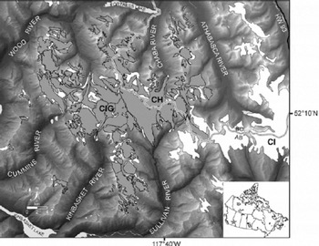
Fig. 1. Map of Clemenceau Icefield Group (CIG) and Chaba Icefield (CH). The grey shaded areas are the CIG/CH glacier boundaries based on 2001 satellite imagery. The white glacier areas (Columbia Icefield (CI) and surrounding CIG/CH) are the permanent snow/ice cover from Natural Resources Canada maps (http://geogratis.cgdi.gc.ca/geogratis/) based on 1985–87 air photos. Wales Glacier (W) has accumulation areas in all three icefield groups. The base image is the resampled and hill-shaded DEM (http://www.geobase.ca/geobase/en/metadata.do?id=15508).
Methods
Glacier outlines, length, slope and retreat
Glacier outlines were manually digitized from 15m orthorectified panchromatic 2001 Landsat 7 ETM+ and georeferenced 2000 and 2001 ASTER level 1B images, using the on-screen ESRI ArcMapTM version 9.2 Geographic Information System (GIS) polygon tools. Ice divides were determined using DEM-derived 20m contour lines (see below), while Google Earth and airborne photographs taken from a helicopter during 2004–08 field campaigns were consulted for steep terrain, debris-covered glaciers and shaded areas. Any rock areas inside the glacier polygons were excluded from the glacier area. Because of the poor gain setting of three of the four ASTER scenes, as well as the early or late snow cover on the October and June images, ASTER scenes were merely used as a verification of the outlines digitized from the 14 September 2001 Landsat 7 scene (path 44, row 24, band 8: 15 m panchromatic). The region in Figure 1 is in the top left quadrant of this Landsat scene.
Each glacier was given a unique five-digit ID indicating hierarchy of Icefield, River Basin, Drainage Basin, Glacier System and Individual Glacier, and, where available, official glacier names were assigned. The first two digits of the CIG glacier ID represent drainage into the Wood River (11 and 15), Cummins River (12), Kinbasket River (13) and Sullivan River (14) and for CH drainage into the Chaba River (21) and Athabasca River (22) (Fig. 1). Within each of these river basins, glacier systems within secondary drainage basins were numbered clockwise from the downstream vantage point. The fourth and fifth glacier ID digits are for individual glaciers and possible tributaries, and allow for grouping by glacier system. All data were projected in North American Datum 1983 (NAD83) Universal Transverse Mercator (UTM) zone 11N, and most glacier attributes were automatically derived in the GIS.
Centre flowlines were digitized manually, and glacier length, maximum and minimum centre flowline elevations were used to calculate average glacier slope. Glacier retreat was measured from the central crest of Little Ice Age (LIA) moraines, and from 1985–87 digital Natural Resources Canada (NRCan) permanent snow/ice cover maps (http:// geogratis.cgdi.gc.ca/geogratis/; Fig. 1), by tracing a past flowline (assumed to follow the centre of the valley) continuing from the margin of the present (2001) glacier flowline. Tributary retreat was measured from the 2001 tributary flowline margin, along the centre valley (former flowline) to the present (2001) or past centre line of the trunk glacier. The LIA maximum in the Columbia Icefield region occurred around the 1840s, but later (1860–80) in the Mount Robson region to the north and the Yoho National Park region to the south (Reference LuckmanLuckman, 2000).We chose 1850 as the LIA maximum for our study region, but indicate uncertainty with error bars. Maps and glacier descriptions of glacier margins from historic climbing reports (e.g. Reference CarpeCarpe, 1923) were also used to assess retreat rates. Computed retreat rates were then compared to glacier characteristics, and to retreat rates in nearby icefields (Reference LuckmanLuckman, 2000; Reference Osborn, Robinson and LuckmanOsborn and others, 2002).
Glacier elevation, ELAs and snowlines
A 2 arcsec NRCan DEM (http://www.geobase.ca/geobase/en/metadata.do?id=15508) based on Terrain Resource Information Management (TRIM) data, maps and air photos, was used to derive elevation, slope and aspect. Five DEM map sheets were projected and resampled to 20x20m using bilinear interpolation, and 20m interval contour lines were extracted. From these, glacier maximum and minimum elevations were derived, taking the upper contour bounding the maximum and minimum elevation of the glacier (maximum error in absolute elevation is therefore the DEM error ±19 m).
The geodetic equilibrium-line altitude (ELA) according to the ‘Hess’ method (ELAH) is assumed to represent the kinematic long-term ELA and can be determined from the transition of convex to concave contour lines in the ablation zone (Reference Leonard and FountainLeonard and Fountain, 2003). The concave contour (up-glacier) was taken as the ELAH elevation, in order to ensure systematic interpolations. Because not all glaciers have clear contour-line transitions, and those with icefalls in the ablation zone or ending in steep cliffs should be avoided, we could apply this method to only 47 glaciers. Another proxy for long-term ELA can be derived using the ‘Kurowski’ method (ELAK), which is the area-weighted mean altitude (Reference KurowskiKurowski, 1891; Reference Braithwaite and MüllerBraithwaite and Müller, 1980), and corresponds to an accumulation-area ratio (AAR) of 0.5 for a symmetric hypsometric curve. The long-term AAR0 for Peyto Glacier, the nearest glacier with long-term mass-balance records (since 1966: WGMS, 2003), is 0.53, suggesting that ELAK might be a good regional proxy for AAR0. ELAK was automatically extracted for all glaciers using glacier area–elevation distributions from the DEM. Additionally, the elevation of a theoretical ELA65 (AAR = 0.65), was extracted for all glaciers as a lower limit of a possible ELA0. The sensitivity of glaciers to changes in mass balance was quantified by the change in AAR, both in percentage and absolute area, in response to a 100 m and a 200m rise in snowline relative to ELAK and ELA65. We further compared the theoretical equilibrium lines (ELAH, ELAK and ELA65) to observed snowlines, which were traced from ice–snow boundaries on interactively stretched panchromatic Landsat 7 images of 14 September 2001, using a threshold DN value of 125 in ArcMap. This threshold, where DN125–255 is snow, was determined through comparison with the visible snowline on Landsat and ASTER images. This method was chosen to achieve consistency in the snowline elevation date, and at the same time retain the 15 m resolution of the panchromatic band (B8) of Landsat 7 ETM+. We used the digitized snowline polylines to mask the DEM by applying a 10m buffer on either side of the snowline and extracting all elevation pixels that fall within the buffered line. In this way, maximum, minimum, average snowline elevation and standard deviation could be determined for each glacier and for the entire region. This method was chosen over converting the snowline polyline into a raster file and extracting DEM values using this raster because (a) the DEM-extracted snowline had up to 50% more pixels with the raster method, and (b) extracted elevation pixels on both ends of the snowline were often outside the glacier boundary when using the raster method. Even though the buffering method was considered more accurate, the average snowline elevation for the entire region was the same for both methods, and the average snowline difference for individual glaciers was only in the order of 0–9 m. Snowlines could be determined for 106 glaciers (some glaciers were all accumulation or ablation area) and are 77–6262m long.
Automatic snow-pillow (ASP) snow water-equivalent (SWE) data at Molson Creek (British Columbia Ministry of Environment River Forecast Centre, http://a100.gov.bc.ca/pub/aspr/) ~25 km west of CIG, indicate that 2001 was one of the lowest snow years (80% of normal) of the 27 year records. This snowline might therefore be representative of future negative mass-balance trends, which have been correlated to reduced winter precipitation rather than increased summer temperature in this region (Reference LuckmanLuckman, 2000). However, between 14 and 30 September 2001 eight positive degree-days and two days with >15mm rain occurred at Molson Creek ASP (1930ma.s.l.). Using a lapse rate of 0.6˚C (100m)–1, an average PDD factor of 5.5 mmd–1 K–1 (Reference Hock and HydrolHock, 2003) and an accumulation gradient of 200mm(100m)–1 (2000/01 Peyto Glacier mass-balance data from WGMS (2003)), it was determined that the snowline could have been 120m higher at the end of the melt season.
Following Reference LuckmanLuckman (2000), a proxy for the change in equilibrium-line elevation since the LIA was taken as half the elevation difference between the LIA toe elevation and the 2001 ice-margin toe elevation. These elevations were derived from DEM minimum elevations extracted from the LIA retreat lines and 2001 centre flowlines, respectively, using the same buffering method as for the extraction of snowline elevation.
Hypsometry, AAR and planar and slope-corrected areas
Glacier hypsometry, the distribution of glacier area over elevation, is important for long-term glacier response through its link with mass-balance elevation distribution (Reference Furbish and AndrewsFurbish and Andrews, 1984), and is determined by valley shape, topographic relief and ice volume distribution. We determined the hypsometry of CIG glaciers in three different ways.
1. Polygon Planar Surface Area (PPA) was automatically derived from the glacier outlines in the GIS, and PPA hypsometry from integrating glacier polygons with their contour lines and extracting polygon areas within each of the 20 m contour intervals for every glacier. In order to compare hypsometries of glaciers with different areas, hypsometric curves were normalized. Additionally, the hypsometric character of each glacier was quantified as a hypsometric index (HI), where
with H max and H min the maximum and minimum glacier elevations and H med the elevation of the contour line that divides the glacier area in half (Reference Jiskoot, Murray and BoyleJiskoot and others, 2000). This results in a single index for each glacier, and allowed grouping of glaciers into five HI categories, from very top-heavy (H<–1.5) through equidimensional (–1.2 < HI< 1.2) to very bottom-heavy (H> 1.5). Snowline and ELA elevations were superimposed on the hypsometric data and AAR calculated for individual glaciers, so that the relative reduction in AAR could be assessed and linked to HI category.
2. Raster Planar Surface Area (RPA) was derived directly from the 20 x20m DEM pixels by masking with the glacier polygons and using the count and summarize functions in ArcMap. RPA hypsometry was calculated by summing pixels within 20 m elevation interval bins, and multiplying these by their pixel area (400 m). Normalized hypsometries were calculated and hypsometric curves plotted following the procedure for PPA hypsometry.
3. Planar (projected) glacier areas (PPA and RPA) have been traditionally used in glacier inventories and mass-balance calculations because of simplicity, ease of extraction (only a map, air photo or satellite image is needed) and consistency. Systematic studies of the influence of the real three-dimensional surface areas of glaciers (i.e. considering increase in area on sloped terrain) on mass balance, total area, hypsometry and area–aspect calculations are lacking. We therefore derived a Raster Slope Corrected Area (SCA), the closest representation of the three-dimensional surface area, by combining the RPA with the DEM surface slope. Surface slope (α) for each DEM raster cell was computed in degrees using Spatial Analyst in ArcGIS. In order to diminish errors due to edge effects in glacier margin cells due to steep surrounding bedrock cliffs, we thresholded the maximum possible slope to the steepest slope found in an icefall. A maximum slope of 55° was found in the icefall of Duplicate Glacier (111112), which was described by Reference MicroysMicroys (1973) as a ‘groaning teetering mess of giant ground-up ice cubes’. Following Reference Rasmussen and FfolliottRasmussen and Ffolliot (1981), SCA was then calculated as:
SCA thus ranges between 400 m2 for flat DEM cells and 697 m2 for a slope of 55˚. SCA hypsometry was calculated by summing all SCAs for individual pixels within 20m contour interval bins, and hypsometries were normalized and curves plotted as for the PPA hypsometry.
Aspect
Glacier mass balance depends mainly on precipitation, air temperature and solar radiation. While the main glacier topographic effects on overall mass balance are captured when using hypsometry in combination with mass-balance curves, the solar radiation component needs to be corrected for slope–aspect relationships in mass-balance models (Reference HockHock, 2005). This influence of slope and aspect on energy balance is latitude-dependent due to the difference in relative influence of each of the mass-balance components as well as the global variation in solar zenith angle, with a general reduction in sensitivity to slope and aspect from lower to higher latitudes (Reference Arnold, Rees, Hodson and KohlerArnold and others, 2006; Reference Sicart, Ribstein, Francou, Pouyaud and CondomSicart and others, 2007). Although not as important as shading effects of surrounding terrain, slope and aspect can have positive and negative impacts on the overall irradiance balance depending on the relative angle to solar zenith and the surrounding terrain Reference Hock(Hock, 2005), as well as on the distribution of wind-drifted snow. While distributed energy-balance models are now applied more often (e.g. Reference Arnold, Willis, Sharp, Richards and LawsonArnold and others, 1996; Reference Machguth, Paul, Hoelzle and HaeberliMachguth and others, 2006), these only account for slope and aspect, and not for the increased surface area on steeper-sloping terrain. We therefore attempt to explore the relative increase in SCA compared to RPA while taking into account terrain aspect. If increases are relatively larger on southeast–southwest-facing glacier terrain in the Northern Hemisphere, then mass balance might be overestimated, as an additional amount of melt will occur on these slopes. In contrast, if these areas face away from the zenith angle, there will be a net reduction in mass balance. However, even if direct radiation is not a factor, steep terrain will have additional increased area through the formation of crevasses and seracs (e.g. in icefalls), so these areas will receive more sensible heat. The use of SCA might therefore improve DEM-based distributed energy-balance modelling.
Aspect in degrees was calculated from the DEM slope data in ArcGIS and then classified into eight 45˚ bins centred around the compass rose directions, and one bin for flat areas (no aspect). A raster file was then created, with each cell corresponding to one of nine aspect classes. For each glacier, as well as for the entire region, the RPA and SCA in each of the aspect classes were calculated in order to determine the overall aspect distribution of the glacier. The absolute area increase in each of the (non-flat) classes as well as the relative increase in each aspect class were then used to assess any changes in aspect distribution from implementing SCA. Further, dominant glacier aspect was automatically derived from the direction bin with the highest percentage of counts. This DEM-derived aspect was then systematically compared to manually derived aspects of the centre flowline in the accumulation and ablation areas, which have traditionally been used to define glacier aspect in glacier inventories.
Results
Area and length changes
We classified 176 glacier systems (53 of them tributaries) ranging in area from 0.04 to 43.6 km2. The glacier size distribution is logarithmic, with 8 glaciers >10km2 and 111 glaciers <1km2. The CIG area diminished from 313 km2 in the late 1980s (Reference Ommanney, Ferrigno and WilliamsOmmanney, 2002; estimated from 1 : 50 000 maps using the percentage ice cover within each UTM grid square (personal communication from S. Ommanney, 2008)) to 271 km2 in 2001, while CH was 97 km2 in the late 1980s and 69 km2 in 2001. Combined, the 2001 CIG/CH area represents 14% of the total glacier area in western Canada (~25 000 km2: Reference Schiefer, Menounos and WheateSchiefer and others, 2008). The area loss is shown in Figure 1 by the white areas adjacent to the CIG/CH glacier outlines. The rates of area loss (CIG: 9% per decade; CH: 19% per decade give only a very rough range of retreat, as (1) some of the ‘glaciated’ areas from 1980s maps were in fact areas of permanent snow, and (2) the extent of each of the regions might have been misinterpreted due to shared accumulation basins (e.g. Wales Glacier). However, if the range in rate of area loss is linearly extrapolated into the future, the CIG/CH glaciers could disappear in the next 100 years. This rate is dependent on individual glacier response time to present and future changes in mass balance, regional glacier hypsometry and the effect of disintegration of ice masses (see Reference Paul, Kääb, Maisch, Kellenberger and HaeberliPaul and others, 2004).
Since our retreat data are limited to only two time periods (LIA–2001 and 1985–2001), we were not able to assess individual responses and short-term fluctuations in detail. However, we divided the CIG/CH glaciers into five length– slope classes that were found to represent typical length fluctuation responses in the Swiss Alps (Reference Jiskoot, Caruso, Minke and PigeonHoelzle and others, 2003), in order to assess potential differences in response to mass-balance fluctuations:
class 1: long, flat, constant long-term retreat (>10 km, <15˚: n = 3)
class 2: intermediate length and slope, large decadal fluctuations (5–10 km, 10–15˚: n = 7)
class 3: steep mountain glaciers, moderate decadal fluctuations, individual response (1–5 km, 15–25˚: n = 44)
class 4: flat mountain glaciers, weak decadal fluctuations, strong overall retreat (1–10 km, <15˚: n = 52)
class 5: high-frequency variability, moderate to large amplitude (<1 km, >15˚, or 1–5 km, >25˚: n = 70).
Since the LIA maximum, CIG glaciers have retreated 2.4 km on average (16±6ma–1, n= 22), while CH glaciers have retreated 1.8 km (12±7ma–1, n = 17) (Figs 2 and 3). Between 1985 and 2001, the average retreat rate increased to 25±17ma–1 (n=22) for CIG and 16±11ma–1 (n = 10) for CH, suggesting an accelerated retreat in the late 20th century (Fig. 4a). Glaciers that do not reflect this accelerated trend retreated onto steep cliffs (e.g. Wales Glacier: 14431) or had/have calving fronts (e.g. 22112), and could have experienced accelerated retreat before the mid-1980s due to topographically induced dry or wet calving. Longer glaciers and those with tributary detachment appear to retreat faster than smaller and less complex glaciers, while steeper mountain glaciers (class 4) have slightly lower retreat rates and less of an accelerated retreat in the 1985–2001 period (Figs 3 and 4b). Of the present 176 glaciers, 53 are tributaries that could separate in the future, or have already done since 2001.
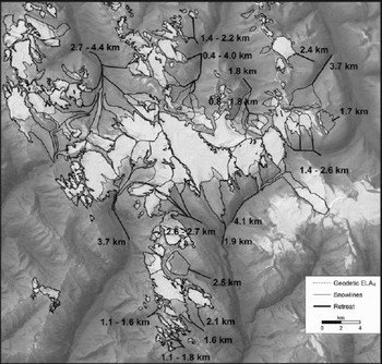
Fig. 2. Glacier retreat map with retreat path from the LIA moraine crest to the 2001 glacier margin. Snowlines and geodetic ELAH are also indicated. Values and ranges indicate the distance that each glacier (cluster) has retreated since the LIA maximum. Note the detachment of tributaries in several glacier systems. Base image is the 14 September 2001 Landsat 7 image, enhanced using the hill-shaded DEM.
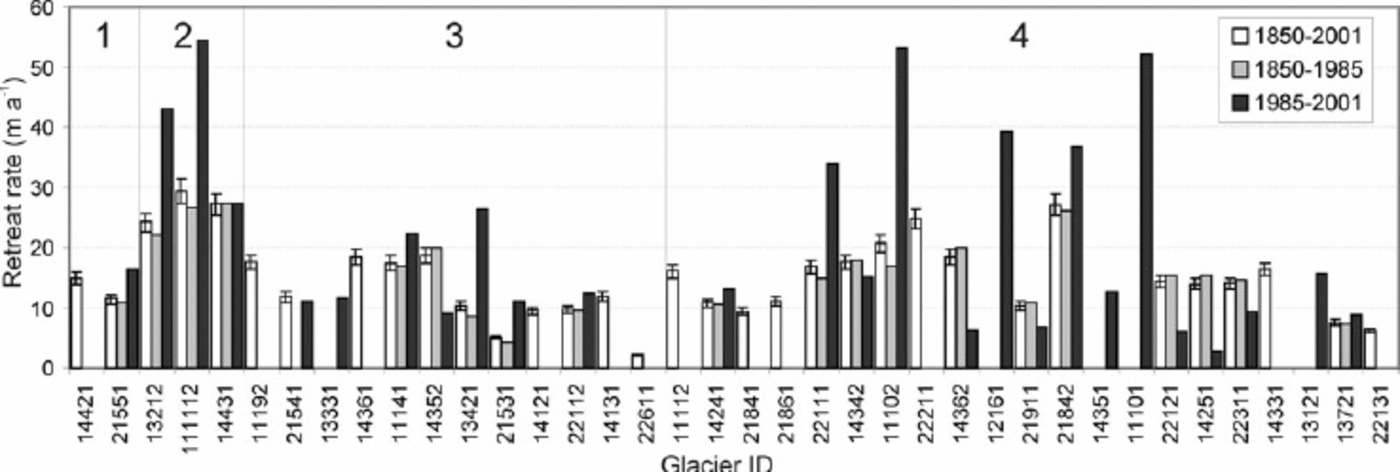
Fig. 3. Glacier retreat rates for 1850–2001 (LIA: white bars), 1850–1985 (grey bars) and 1985–2001 (black bars). Negative error bars in LIA retreat rates are for the LIA maximum occurring in 1840 rather than in 1850, and positive error bars if a 10 year stagnation in retreat occurred in the period 1955–75 (Reference LuckmanLuckman, 2000; Reference Osborn, Robinson and LuckmanOsborn and others, 2001). Numbers 1–4 are the length–slope groups from Reference Jiskoot, Caruso, Minke and PigeonHoelzle and others (2003); within these groups glaciers are sorted on decreasing length. Note accelerated retreat rate in 1985–2001 for 12 of 21 glaciers.
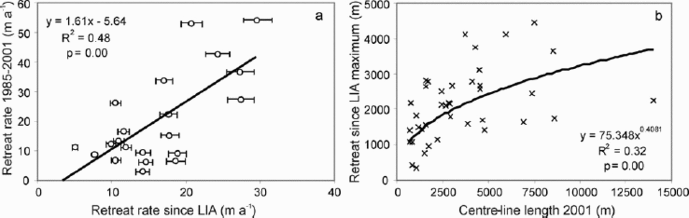
Fig. 4. (a) Relative increase in retreat rate between 1850–2001 and 1985–2001. Horizontal error bars for LIA are identical to vertical error bars in Figure 3. (b) Exponential correlation between glacier length and retreat since LIA, indicating that longer glaciers have retreated more than shorter glaciers.
Hypsometry, ELAs and snowline
The elevations of ELAK, ELA65, ELAH, the 2001 snowline and a late 1980s snowline (Ommanney, 2002) are given as averages for CIG and CH in Table 1, and for individual glaciers in Figure 5. No significant difference was found between median elevations (ELAK) of CIG and CH. The elevation distribution of median elevation with aspect shows only a marginally significant difference between a southeastern aspect (higher) and a western aspect (lower) (Fig. 6), suggesting limited orographically related differences in precipitation and insolation in this region.
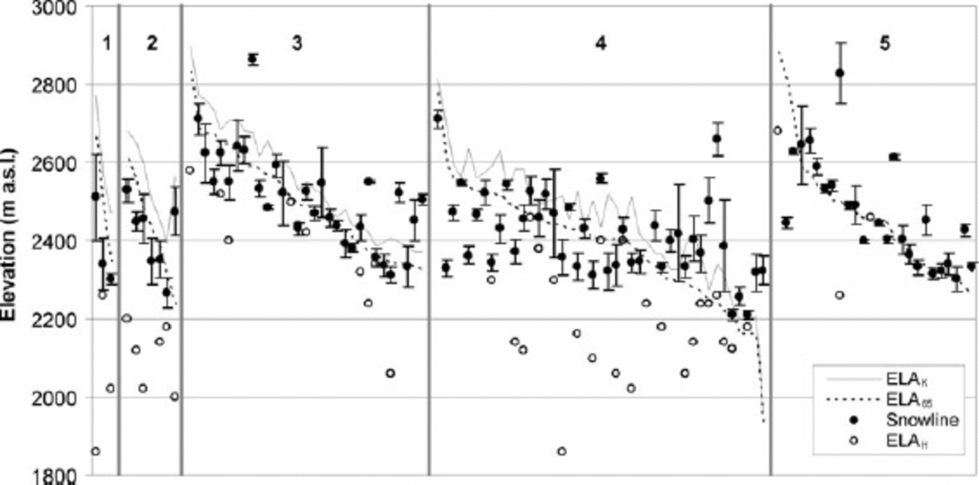
Fig. 5. Elevation distributions of ELAK, ELA65, ELAH and 2001 snowline for 110 CIG and CH glaciers, grouped according to length–aspect classes (Reference Jiskoot, Caruso, Minke and PigeonHoelzle and others, 2003) and within these classes sorted by decreasing altitude of median elevation (ELAK).
Table 1. Average elevations (m a.s.l.) and standard deviations of ELAK, ELA65, ELAH and the 14 September 2001 snowline, as well as a late-1980s snowline Reference Ommanney, Ferrigno and Williams(Ommanney, 2002) and the inferred 30 September 2001 late-summer snowline (14 September snowline + 120 m)
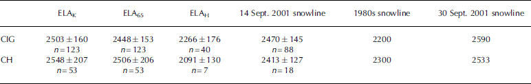
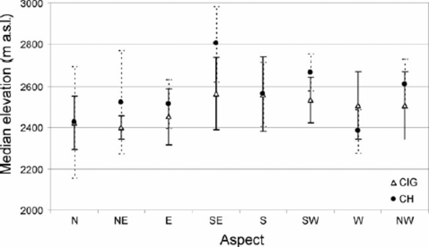
Fig. 6. Average median glacier elevations and standard deviations for CIG and CH grouped by individual compass rose octants.
Figure 5 shows that ELAH is at significantly lower elevation than ELA65, hence glaciers are far from their dynamic equilibrium. It should further be noted that the 2001 snowline is at the same elevation as ELA65, or even lower (mainly for classes 1 and 4), for most glaciers. This suggests that these glaciers had an AAR≥0.65 on 14 September 2001. However, as indicated in the Methods section, the snowline at the end of the hydrologic year would have been ~120m higher, which suggests a 2001 AAR0.5 for most smaller and steeper glaciers (classes 3 and 5), but an AAR of 0.5–0.65 for most larger and flatter glaciers (classes 1, 2 and 4). Peyto Glacier’s AAR was only 0.26 and its ELA 130m above ELA0 (0.53) in the 2000/01 season (WGMS, 2003). This suggests that AAR0 for larger and flatter CIG/CH glaciers would be closer to 0.65, hence the ELA0 closer to ELA65 than ELAK. Further, from the rise in glacier toe elevation between the LIA maximum and 2001 we derive that the ELA0 has risen by 179±92m since the LIA (n = 36: mostly larger glaciers; calving glaciers and those retreating beyond steep cliffs were excluded). This compares to an elevation difference of 206±170m between ELA65 and ELAH. These results suggest that a 100 or 200m rise in snowline is a reasonable approach to assessing the sensitivity to expected changes in mass balance.
Glacier hypsometries are top-heavy for most outlet glaciers, while many of the smaller glaciers are equidimensional or slightly bottom-heavy (Fig. 7). HI ranges from –4.1 to +4.0, while for the entire CIG/CH region it is –1.0 (equidimensional). The outlet glaciers in particular are predicted to be very sensitive to climate change, as a small rise in snowline elevation exposes large additional areas to enhanced ablation, resulting in a smaller AAR (Fig. 7). The rise between average ELAH and average 2001 snowline exposes 5–47% additional ablation area, with an average decrease in AAR of 0.24 for CIG/CH.
Fig. 7. (a) Map with hypsometric indices and select hypsometric curves with relative positions of geodetic ELAs and snowlines. A* is normalized glacier area and Z* normalized glacier elevation. (b) Hypsometric curve for CIG/CH indicating a decrease in AAR of 0.24 due to the rise in ELA.
A 100 or 200m unit rise in ELA relative to the ELAK (AAR = 0.5) and ELA65 (AAR = 0.65) of individual glaciers results in a wide-ranging decrease in AAR. No correlation was found between HI and decrease in AAR, even when considering elevation or length–slope class (Reference Hoelzle, Haeberli, Dischl and PeschkeHoelzle and others, 2003). HI might be too simple a representation of the full glacier hypsometry for this assessment. Using the full hypsometric data to calculate changes in AAR shows that 5–28% of glaciers will lose the accumulation area for a rise in snowline of 100–200m (Table 2). For the entire CIG/CH region a 100 m rise in snowline relative to ELAK will result in an AAR of 0.35, while a 200 m rise results in an AAR of only 0.26. Snowline rise relative to ELA65 results in AARs of 0.51 and 0.39, respectively. Table 2 further shows that very top-heavy glaciers are more affected by progressive changes in snowline than very bottom-heavy glaciers. A rise of 200m relative to a rise of 100 m doubles the loss in accumulation area for top-heavy glaciers, whereas it increases the loss in accumulation area for bottom-heavy glaciers by only a third.
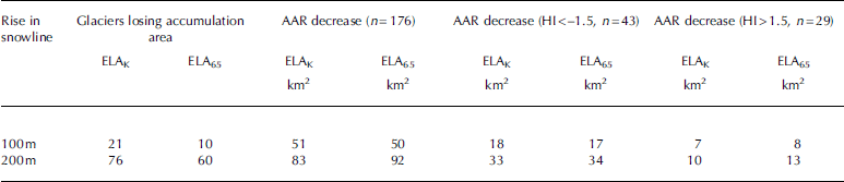
Table 2. Changes in CIG/CH glaciers as a result of a unit 100m and 200m rise in snowline relative to ELAK and ELA65. HI < –1.5 are extremely top-heavy glaciers, and HI > 1.5 extremely bottom-heavy glaciers
Planar area vs slope-corrected area related to hypsometry and aspect
For the entire CIG the PPA and RPA are 347 km2 (the two flow units of Wales Glacier that are actually part of Columbia and Chaba Icefields are included in these calculations, but were excluded for the purpose of PPA comparison with historic CIG area earlier in this paper), while the SCA is 369km2. Hence, if area is measured without applying slope correction at the scale of this icefield, an area underestimation error of 6% occurs (Fig. 8a). While ~50% of the glaciers have an SCA that is <10% larger than the PPA or RPA, for some glaciers it can make a difference of up to 20% (Fig. 8b). The general shape of the hypsometric curves, and hence the HIs, does not significantly differ between PPA, RPA and SCA if each is normalized relative to their maximum area. This means that analyses of hypsometry–mass-balance relationships (Fig. 7) are similar for all three area calculations. However, individual 20m elevation intervals can increase >40% in SCA area for individual glaciers (Fig. 8d–f).
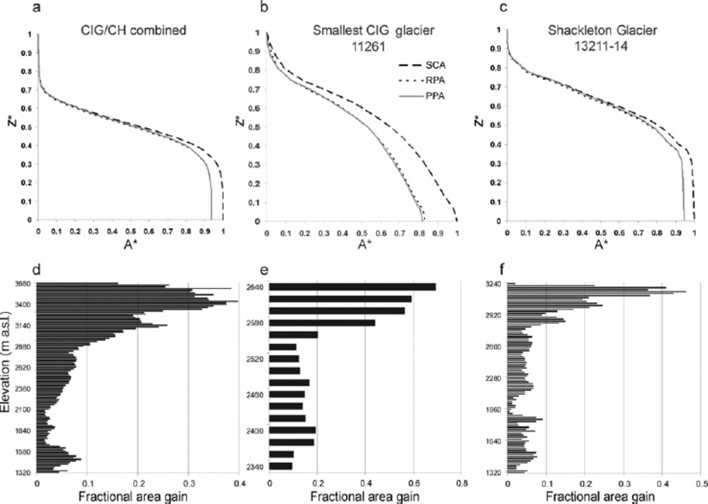
Fig. 8. PPA, RPA and SCA hypsometric curves normalized to SCA total area. (a) All CIG glaciers (PPA= 277 km2; SCA = 295km2); (b) smallest CIG glacier (PPA = 0.064 km2; SCA = 0.077 km2); (c) Shackleton Glacier system (PPA= 43.66 km2; SCA = 45.86 km2). (d–f) Fractional area gain in SCA in each 20m elevation bin relative to the RPA in that bin. Higher regions as well as icefalls gain relatively more area.
Glacier aspect is generally classified as the overall flowline direction, or that of the flowline in the accumulation and ablation zones. Since many glaciers have more complex aspect–area distributions (Fig. 9a), this approach might distort regional mass-balance modelling attempts. With the improved DEM resolutions it is now possible to derive the dominant aspects of the upper and lower parts of the glacier directly from the full range of DEM aspects. However, a method has not been standardized, and can range from simply taking the dominant aspect class to taking average direction using the full range in aspects (e.g. Reference Schiefer, Menounos and WheateSchiefer and others, 2008). We tested the first method and compared this to flowline directions in accumulation and ablation regions, and found that 85–90% of DEM-derived aspects coincide within one eight-point compass rose direction with either the accumulation or ablation flowline aspect (e.g. DEM-derived aspect = W, flowline direction = W, SE or SW), and <1% deviate three or four compass rose directions (e.g. DEM-derived aspect = W, flowline direction = N, S, NE or NW). Ideally, for mass-balance purposes, the full range of aspects is considered.
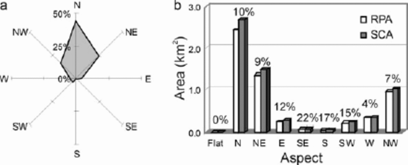
Fig. 9. Clemenceau Glacier aspect data from DEM. (a) RPA glacier aspect distribution in percent of total glacier area. Flat area is 0.1%. (b) Areas in km2, and relative increases in percent (numbers above bars) between RPA and SCA.
Using the full range in aspect from the DEM, we assessed whether SCA area increase was disproportionate in certain aspect classes. For the entire CHIG/CH region, increases were evenly distributed, but for individual glaciers this is not always the case. For example, for Clemenceau Glacier (11161) the percentage increase in area varies widely over the aspect octants (4–22%: Fig. 9b). Even if the overall aspect–area distribution were to remain the same in SCA, the absolute increases in area might have some effect on the overall glacier energy balance, but without additional data on topographic shading and solar incident angle we cannot make conclusive statements about the sign or the amount of this effect.
Discussion and Conclusions
The 9% rate of area loss per decade for CIG between 1985 and 2001 is significantly lower than that for the European Alps in the same period (15% per decade: Reference Paul, Kääb, Maisch, Kellenberger and HaeberliPaul and others, 2004), while the 19% area loss per decade for CH is slightly higher. Both CH and CIG have higher area loss rates than glaciers in Norway (6% per decade: Reference Andreassen, Paul, Kääb and HausbergAndreassen and others, 2008) and in other parts of the Canadian Cordillera (3% per decade: Reference DeBeer and SharpDeBeer and Sharp, 2007). Some of the northern CIG outlet glaciers have retreated >4 km since the LIA maximum (20–30ma–1), >2 km between 1923 (map in Reference CarpeCarpe, 1923) and 2001, and 600–800m since 1985 (30–55ma–1). Compared to glaciers in the Columbia Icefield region, this is double the retreat of Athabasca and Saskatchewan Glaciers, almost double that of Peyto Glacier Reference Ommanney, Ferrigno and Williams(Ommanney, 2002), but comparable to Stutfield Glacier (20ma–1 in the period 1948–92, with 5 year averages between 12 and 36ma–1: Reference Osborn, Robinson and LuckmanOsborn and others, 2001). For Chaba Glacier, the only glacier in our region with field-based retreat measurements (19ma–1 between 1927 and 1936: Reference McCoubreyMcCoubrey, 1938), we measured a significantly lower retreat rate since the LIA maximum (12ma–1), but a comparable retreat rate (17ma–1) for the period 1985–2001. We postulate that the higher average retreat rates for CIG/CH than for Columbia Icefield glaciers are the result of five possible differences between the icefield regions, namely hypsometry, mass-balance gradient, area–aspect distribution, glacier length and tributary detachment.
Yearly ablation measurements (2004–08) on Shackleton Glacier (13211–14) yield an ablation gradient of ~1.2m (100 m)–1, which is slightly steeper than on Peyto Glacier (Reference Demuth, Keller, Demuth, Munro and YoungDemuth and Keller, 2006), suggesting that glaciers west of the continental divide have a higher activity index and could therefore be more sensitive to climate change. Because winter precipitation is the main mass-balance factor in this region (Reference LuckmanLuckman, 2000), the recent reduction in snowfall (Reference BrownBrown, 2000) might also have affected these glaciers more than those on the lee side of the Rockies. Additionally, the general aspect of CIG is more towards the southwest to southeast than the general aspect in the southern Rockies (Reference Schiefer, Menounos and WheateSchiefer and others, 2008). This might result in increased ablation due to more direct solar irradiance on an earlier snow-free glacier surface. Finally, detachment of tributaries could potentially result in accelerated retreat because longwave radiation received from surrounding (dark) bedrock can increase the melt close to the glacier edge (Reference Fountain and VecchiaFountain and Vecchia, 1999; Reference HockHock, 2005).
The finding that longer or larger glaciers are retreating faster (or lose more area) has also been reported for a number of other regions (e.g. Reference Paul, Kääb, Maisch, Kellenberger and HaeberliPaul and others, 2004; Reference DeBeer and SharpDeBeer and Sharp, 2007; Reference Andreassen, Paul, Kääb and HausbergAndreassen and others, 2008). Reference DeBeer and SharpDeBeer and Sharp (2007) suggested that this size dependence of mass loss can be explained by the fact that larger glaciers extend further down in the valleys and hence experience higher temperatures, while smaller glaciers have retreated to well-shaded steep-walled high places. Further, larger glaciers may also be more sensitive to climate change due to their lower slopes because of mass-balance–altitude–topography relationships Reference Oerlemans(Oerlemans, 1989), although they might at the same time react slower due to longer dynamic response time. The dynamic response of glaciers to climate forcing is strongly dependent on initial size and geometry (Reference Kuhn and OerlemansKuhn, 1989). Initial glacier length and slope determine whether retreat rates could be interpreted as adjustment to secular, decadal or annual variations in mass balance (Reference Hoelzle, Haeberli, Dischl and PeschkeHoelzle and others, 2003). Using Rocky Mountain glaciers, we found similar retreat rate variations between glaciers with different length–slope characteristics (Fig. 3) to those found by Reference Jiskoot, Caruso, Minke and PigeonHoelzle and others (2003) in the Swiss Alps. We also found that glaciers terminating in lakes or on steep cliffs behaved anomalously due to topographic constraints. On the basis of the data presented in this paper we suggest that glacier hypsometry (mostly top-heavy for the larger outlets) and tributary detachment might also contribute to larger glacier systems retreating faster.
In summary, this CIG/CH glacier inventory research yields the following results:
CIG has an area of 271 km2 and lost 42 km2 or 9% per decade between the mid-1980s and 2001. CH has an area of 69 km2 and lost 28 km2 or 19% per decade since the mid-1980s.
The average retreat rate of CIG/CH glaciers has increased from 18 ma–1 in the period 1850–2001 to 30 ma–1 in the period 1985–2001.
Within the 176 glacier systems, there are still 53 tributary units, and detachment of these might increase the retreat rate further.
Rise in ELA between the LIA and the early 21st century was in the order of 200 m.
A future upward snowline shift of 100 or 200m will result in a further 50–92km2 expansion of the regional ablation area, which is 15–27% of the present glaciated area. Between 21 and 76 glaciers will lose their accumulation area altogether.
Outlet glaciers have top-heavy hypsometry while smaller glaciers are mainly equidimensional.
Polygon Planar Surface Area (PPA) and Raster Planar Surface Area (RPA) underestimate the Slope Corrected Area (SCA) by 5–20%, but do not significantly change the hypsometry of the glacier.
SCA calculated for eight aspect categories substantially increases the area in select compass directions for individual glaciers. Further research, using a distributed energy-balance model is needed to assess the effects of these aspect–area discrepancies on glacier mass balance.
Acknowledgements
We thank S. Kienzle and G. Duke for GIS support, S. Ommanney for clarification of previous inventory work, and the Global Land Ice Measurements from Space (GLIMS) program for providing access to ASTER data and inventory procedures. The critical and thorough review of an anonymous reviewer helped improve the paper, and scientific editor R. Braithwaite provided additional information on the Kurowski method. This research was funded through a Natural Sciences and Engineering Research Council (NSERC, Canada) Discovery Grant to H.J.


