


Introduction
The continued accumulation of greenhouse gases in the atmosphere is one of many reasons for global climate modifications. In the last few years there has been an intensification of interest in climate change, partly because of extreme events, including summer droughts in the United States and Europe and milder winter conditions in the regions of cold climate. General circulation models are a prime tool for studying the current climate and the changes to it due to an increase of greenhouse gases. Results from various mathematical models of the climate system show that warming of the troposphere as a consequence of increasing carbon dioxide (CO2 ) can be expected, assuming that all other components of the system remain unchanged (Reference Hansen, Hansen and TakahashiHansen and others, 1984, Reference Hansen1988; Reference Washington and MeehlWashington and Meehl, 1984; Reference Wetherald and ManabeWetherald and Manabe, 1986; Reference Wilson and MitchellWilson and Mitchell, 1987; Reference Rind, Goldberg and RuedyRind and others, 1989; Reference Schlesinger and ZhaoSchlesinger and Zhao, 1989; Reference Manabe, Stouffer, Spelman and BryanManabe and others, 1991; Reference Meehl, Washington and KarlMeehl and others, 1993).
Numerous simulations of the possible climatic changes which could occur under equilibrium (2 × CO2) greenhouse conditions have been carried out by several groups (Reference Hansen, Hansen and TakahashiHansen and others, 1984, Reference Hansen1988; Reference Washington and MeehlWashington and Meehl, 1984; Reference Wetherald and ManabeWetherald and Manabe, 1986; Reference Wilson and MitchellWilson and Mitchell, 1987; Reference Rind, Goldberg and RuedyRind and others, 1989; Reference Schlesinger and ZhaoSchlesinger and Zhao, 1989; Reference Manabe, Stouffer, Spelman and BryanManabe and others, 1991; Reference Meehl, Washington and KarlMeehl and others, 1993; Reference Gordon and HuntGordon and Hunt, 1994). Greenhouse gas experiments have been reviewed by Reference Schlesinger and MitchellSchlesinger and Mitchell (1987), Reference MitchellMitchell (1989) and Reference Houghton, Jenkins and EphraumsHoughton and others (1990).
The experiment discussed here explores simulated climatic change at equilibrium in a 2 × CO2 experiment. A three-dimensional NASA Goddard Institute of Space Studies (GISS) atmospheric general circulation model (Reference HansenHansen and others, 1997) coupled to a mixed-layer ocean and thermodynamic sea-ice model is used. The mixed-layer ocean model allows sea-surface temperature (SST) to change as a result of atmosphere-ocean heat-flux exchange but with implicitly prescribed climatological ocean heat transport (the so-called "Q-flux" approach). These coupled atmosphere-mixed-layer ocean models have been extensively used for CO2 increase experiments (Reference Wilson and MitchellWilson and Mitchell, 1987; Reference HansenHansen and others, 1988; Reference Gordon and HuntGordon and Hunt, 1994) and paleoclimate simulations (Reference Kutzbach and GallimoreKutzbach and Gallimore, 1988; Reference Mitchell, Grahame and NeedhamMitchell and others, 1988).
The purpose of this paper is to examine the equilibrium response of the Northern Hemisphere climatology in the NASA GISS coarse-grid global coupled climate model. We illustrate simple aspects of interannual and seasonal variability in the model and observations by looking at geographic patterns of surface air temperature, sea-level pressure, precipitation and sea-ice extent for the Northern Hemisphere. The current climate (1 × CO2: control run) is compared with the new equilibrium climate obtained after a gradual increase of carbon dioxide (an exponential transient increase of 1 % per year until the CO2 amount doubled). We compare the Northern Hemisphere sea-ice areas and thickness to observed ice-area data (NSIDC, 1997) and central Arctic ice-thickness data (Reference Rothrock, Yu and MaykutRothrock and others, 1999), as well as the control and CO2 results of sea-ice quantities for the Northern Hemisphere and central Arctic. We also discuss seasonal changes of the Arctic sea-ice extent under doubled CO2 climate forcing.
The Coupled Model
The coupled atmosphere-mixed-layer ocean model used in this study is the Q.-flux version of the GISS global climate model described by Reference HansenHansen and others (1997), with some modifications of the atmospheric model. The horizontal resolution of the model is set as 4° latitude × 5° longitude both in the atmosphere and in the ocean. In this model, an improved four-layer thermodynamic sea-ice model is employed and the atmosphere has 12 vertical layers with the three added layers in the upper troposphere and stratosphere. The Q-flux ocean model (Reference Hansen, Hansen and TakahashiHansen and others, 1984; Reference Wilson and MitchellWilson and Mitchell, 1987) is one member of a hierarchy of ocean representations, ranging from observed ocean temperatures to fully prognostic dynamical models that are being attached to the same atmospheric model. The ocean has a monthly-varying mixed-layer depth and specified horizontal transport of heat, thus permitting SST to be simulated. The mixed-layer oceanic transports were computed in a preliminary model run which used the observed monthly mean SSTdistribution.
Starting from the state reached at the end of the preliminary integration, the mixed-layer model was integrated further, allowing the temperature of the mixed-layer ocean to change thermodynamically. Calculations of changes in thickness of the four-layer ice and snow layers are based on energy balances at the various interfaces (Reference Parkinson and WashingtonParkinson and Washington, 1979); snow is accumulated at the rate computed in the atmospheric model. The albedo of snow ice depends on surface temperature, snow and ice thickness and snow age. The melting begins from the top and bottom surfaces of the snow-ice slab. If the computed top or bottom surface temperatures are > 0°C, it is set to 0°C, and the excess heat accumulated at the snow-ice surfaces is used to melt the snow ice. If the snow ice melts completely, the heat flux from the atmosphere goes to the warming of the ocean surface.
Two 150 year integrations of the coupled model were performed. The CO2 concentration remains unchanged in the first integration (the control run). In the second integration the atmospheric concentration of carbon dioxide increased at a rate of 1 % per year for 70 years. The initial conditions for both integrations have realistic seasonal and geographical distributions of SST and sea ice, with which both the atmospheric and oceanic components of the model are nearly in equilibrium. This equilibrium condition for the control run was obtained by separate integration of the atmospheric model using observed surface conditions (SST and sea-ice concentration). The CO2 experiment was started from the nearly equilibrium state of the control run, which was chosen after about 30 years of integration. CO2 concentration achieved double the initial concentration after about 70 years of integration, and then it remained at this level. The model was integrated for another 75 years. We have evaluated the influence on the coupled system of gradually increasing atmospheric carbon dioxide from the difference between the second (transient 1% per year CO2 increase) and the first (control) integrations. For this purpose we consider the last 20 years of both integrations where the equilibrium of the CO2 experiment was reached.
Results
Climate simulation with Q.-flux ocean and thermodynamiconly sea-ice model has some limitations. The fully dynamical ocean models allow for circulation changes in the ocean, which include the meridional overturning component, the gyre component, such as the mid-latitude gyres in the North Pacific and North Atlantic, and sub-grid-scale lateral diffusion. The mixed-layer model neglects the effects of possible slowing down of the meridional circulation, which cools the North Atlantic. As a result, the Q.-flux model has warmer-than-observed tropical SSTs and cooler-than-observed high latitude, causing over-extensive sea ice. Because of warm tropical SSTs and over-extensive sea ice, the mixed-layer model is very sensitive to CO2−induced warming, which was noticed in analysis of mixed-layer and fully dynamical ocean simulations by Reference Washington, Meehl and SchlesingerWashington and Meehl (1991). Absence of sea-ice dynamics contributes further to the over-extensive sea-ice cover, not allowing export of sea ice out of the Arctic Ocean. The comparison of model integrations with and without sea-ice dynamics was performed by Reference Pollard and ThompsonPollard and Thompson (1994), who noticed that the overall pattern of sea-ice area bears much less resemblance to reality than that with dynamical ice (Reference Weatherly, Briegleb, Large and MaslanikWeatherly and others, 1998).
The ability of a climate model to simulate the change of climate caused by doubling CO2 depends in part on how well it reproduces the present climate and its change from winter to summer. In order to assess the simulation capability of the present model, several quantities for the Northern Hemisphere will be shown and compared with observed data.
The unforced control simulation exhibits multi-decadal warming and cooling episodes, with global temperature change up to 0.35°C, as well as shorter-period fluctuations. The largest variations occur over periods of several decades, but substantial changes often occur within a few years, with the sea-ice changes commonly associated with global temperature change. In the Northern Hemisphere the largest year-to-year variations occur in Baffin and Hudson Bays, in the Barents and East Siberian Seas, in the Sea of Okhotsk and in the Bering and Beaufort Seas. The global surface air temperature has a high correlation (0.82) with the Arctic surface temperature, with the Arctic temperature lagging the global temperature by 2 years. The highest correlation of global temperature and sea-ice extent (-0.52) occurs when the sea-ice extent lags global temperature by 1 year.
Figure 1 shows the observed (Reference Shea, Trenberth and ReynoldsShea and others, 1990) and simulated surface sea-level pressure over the Arctic for December-February (DJF) and June-August (JJA). In winter (Fig. 1a and b), the North Atlantic low extends northeastwards over the Greenland and Barents Seas. Winter high-pressure systems over the American and Eurasian continents link across the Arctic. Over the North Pacific lies the high-pressure system called the Aleutian low. In the summer (Fig. 1c and d), the low-pressure system extends across the Arctic, linking the high-pressure systems in the Pacific and Atlantic. In winter, low precipitation values he along the high-pressure ridge over the central Arctic (Fig. 2a), while the model shows an increase of precipitation in the central Arctic during summer (Fig. 2b). The annual mean Arctic precipitation minus evaporation is consistent with the European Centre for Medium-range Weather Forecasts analysis field given by Reference Briegleb and BromwichBriegleb and Bromwich (1998) (not shown).

Fig. 1. Sea-level pressure: (a) DJF observed (Reference Shea, Trenberth and Reynoldsshea and others, 1990); (b) DJF modeled minus control run; (c) JJA observed (Reference Shea, Trenberth and Reynoldsshea and others, 1990); ( d) JJA modeled minus control run.

Fig. 2. Modeled minus control run precipitation: (a) DJF; (b) JJA.
Surface air temperature over the Arctic, observed (Reference Rigor, Colony and MartinRigor and others, 2000) and simulated for DJF and JJA, is shown in Figure 3. Observed surface air temperatures from the International Arctic Buoy Programme/ Polar Exchange at the Sea Surface (Reference Rigor, Colony and MartinRigor and others, 2000) have higher correlations and lower rms errors than previous surface air-temperature fields from land stations and the Russian North Pole drift stations and provide better temperature estimates, especially during summer in the marginal ice zones. The coldest surface air temperature in DJF is over the Greenland ice cap and the Siberian land where the lowest mean temperatures are below −40°C (Fig. 3a and b). Over the Arctic Ocean, the coldest air is modeled on the northern sides of the Siberian coast and Canadian Archipelago. Relatively warm air penetrates the Arctic from the North Atlantic through the northeastward extension of the Icelandic trough. In summer (Fig. 3c and d), surface air temperature is much higher than in winter, with warm air (>0°C) around all coastlines and outside of the central Arctic. Nevertheless, the model reproduces surface air temperature a little too low over the central Arctic compared to the data.

Fig 3. As figure 1, but for surface air temperature. observed fields are derived from the dataset of Reference Rigor, Colony and Martinrigor and others (2000).
The doubled CO2 experiment reveals that the current GISS mixed-layer Q-flux model continues to have high sensitivity with about 4°C global warming. This compares with a range of simulated temperature increase of 1.9−5.2°C obtained with climate models of this kind (Reference Mitchell, Grahame and NeedhamMitchell and others, 1988). The warming is greatest around sea-ice margins in winter and least over sea ice in summer. There is little seasonal variation in the warming of the tropics. Temperatures increase more over land than over the ice-free ocean. The annual mean warming is greatest at high latitudes, which has been noted in other simulations and has been attributed mainly to sea-ice and snow albedo feedback (Reference Manabe and StoufferManabe and Stouffer, 1980; Reference Ingram, Wilson and MitchellIngram and others, 1989). This feedbac-mechanism requires sufficient warming to cause substantial melting of snow and ice at high latitudes. The resulting decrease of albedo then permits further warming, more melting of ice and snow, and so on. The melting of ice and the heat stored in the ocean mixed layer during the summer as a result of CO2−associated tropospheric warming contribute to less sea-ice formation during the following winter and a poleward shift of the ice margin. The mixed-layer ocean continues to release heat at latitudes of ice-free ocean in the doubled CO2 case throughout the winter, as evidenced by the large warming at the ice margins.
This effect is evident in Figure 4 where surface air-temperature changes resulting from doubling of the CO2 are illustrated for DJF and JJA averaged over the last 20 years of simulations. These results are very similar to other model outputs (Reference Schlesinger and MitchellSchlesinger and Mitchell, 1987; Reference Gordon and HuntGordon and Hunt, 1994). The surface air temperature increased by 2−4°C, with larger warming at high latitudes. In both polar regions, temperature rises of > 10°C were obtained during winter owing to the melting of sea ice. The warming over land in the Northern Hemisphere is greater during winter, although higher warming occurs over North America during the summer. It is interesting to notice that the model displays slight cooling (about −0.5°C) of surface air over Europe. This result indicates that severe regional cold can still occur even under enhanced greenhouse conditions.

Fig. 4. Surface air-temperature change (greenhouse experiment minus control), averaged over the last 20 years of simulations: (a) DJF; (b) JJA.
The mean (over the last 20 years of integration) of monthly Northern Hemisphere sea-ice areas from Q-flux control and C02 experiments, as well as from satellite data (NSIDC, 1997), is shown in Figure 5a. The satellite values were interpolated to the model grid. The Northern Hemisphere sea-ice area from the control run is 20−25% greater than the satellite values in January-September, and it is consistent with the satellite data in October-December (Fig. 5a). The excessive modeled ice cover could partially be explained by the possible underestimation of sea-ice area in the satellite data due to the technical difficulty of distinguishing melt ponds and open water. Sea-ice area decrease resulting from doubling of the CO2 has a maximum of 70% for the Northern Hemisphere in August, with a smaller decrease in winter. The area-averaged thickness, defined as the area-weighted mean of ice thickness in the ice-covered fraction of each gridcell, is shown in Figure 5b for the control and CO2 experiments. The control run reproduces the seasonal cycle of ice thickness with a maximum of 1.6 m in May and minimum of 1.3 in October. Our Q-flux model shows a small seasonal cycle which can be seen from the comparison of sea-ice thickness in the central Arctic (Fig. 5c). The ice-thickness data from Reference Rothrock, Yu and MaykutRothrock and others (1999) represent the modeled seasonal cycle of ice thickness over the central Arctic from an ice-ocean model with a 12−category ice-thickness distribution (Reference Zhang, Rothrock and SteeleZhang and others, 1998). This seasonal cycle was modeled over 40 years of data-release area in the central Arctic. The annual mean ice thickness in the central Arctic (Reference Rothrock, Yu and MaykutRothrock and others, 1999) is about 3.5 m, while our control run has an annual mean ice thickness of about 2.75 m with a small seasonal cycle. The absence of sea-ice dynamics is one limitation of the Q.-flux model, which might be a reason for the reduction of the sea-ice thickness seasonal cycle. Sea-ice thickness decrease resulting from doubling of the CO2 has a maximum of 55% for the Northern Hemisphere in August. An ice slab has a smaller annual thickness range of roughly 0.5 m, while the thinning in the central Arctic (Fig. 5c) is about 2 m, with maximum decrease of ice thickness in summer (76%).
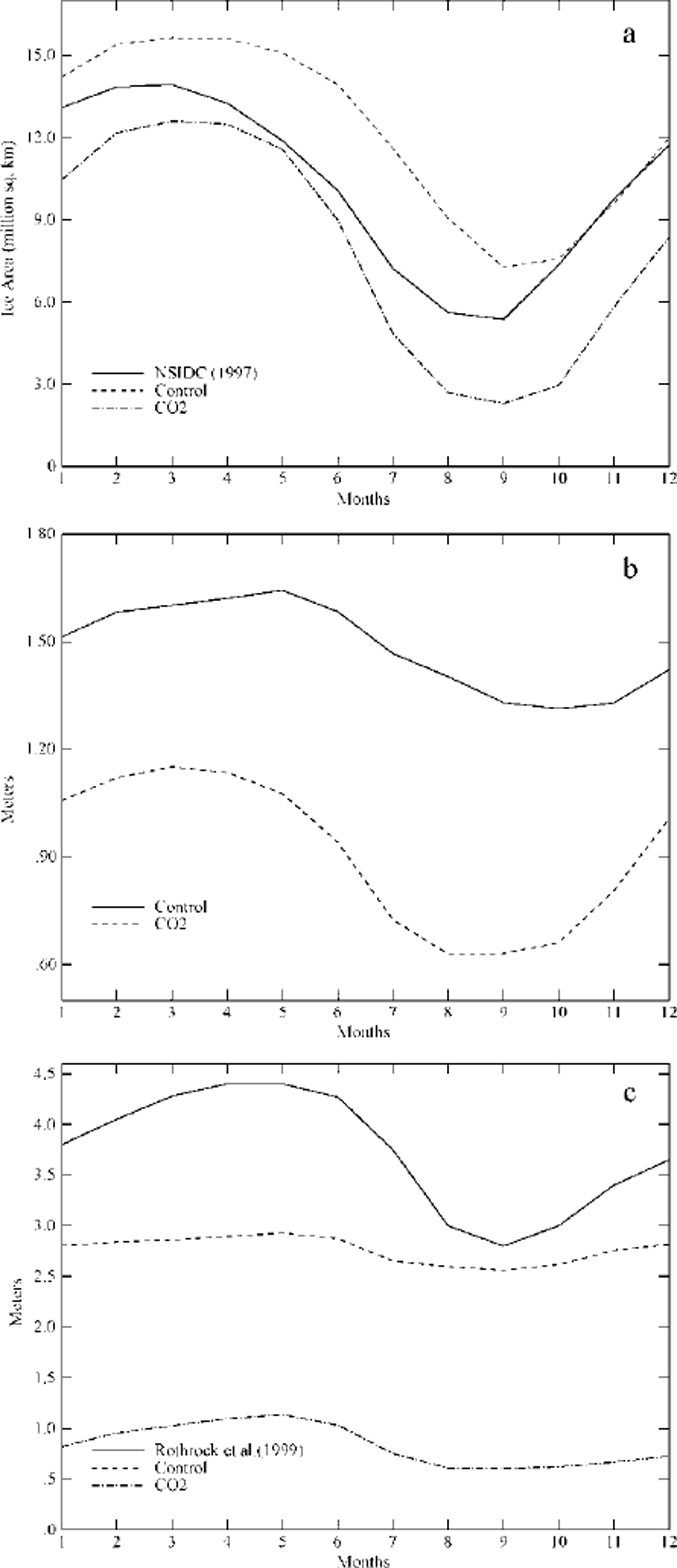
Fig. 5. Mean annual cycle (over last 20 years of integration) of monthly northern hemisphere sea ice: (a) ice area; (b) ice thickness; (c) ice thickness for the central arctic. observed fields are derived from NSIDC (1997) and Reference Rothrock, Yu and Maykutrothrock and others (1999).
Mean ice concentrations from the 20 year climatology for August are shown in Figure 6 for the control and CO2 experiment. The motionless concentrations form more or less concentric circles centered nearly on the pole, corresponding to the nearly zonal isotherms in the atmosphere. This fact was noticed by Reference Pollard and ThompsonPollard and Thompson (1994) after the comparison simulations with and without ice dynamics. Shaded areas are concentrations of > 0.25. The control model does not show much retreat of the sea in the Arctic Ocean (Fig. 6a), while the CO2 experiment exhibits extensive reduction of sea-ice concentration in the central Arctic (Fig. 6b). The annual mean sea-ice reduction due to doubled CO2 is about 30% for the Northern Hemisphere, similar to the results of Reference Pollard and ThompsonPollard and Thompson (1994).
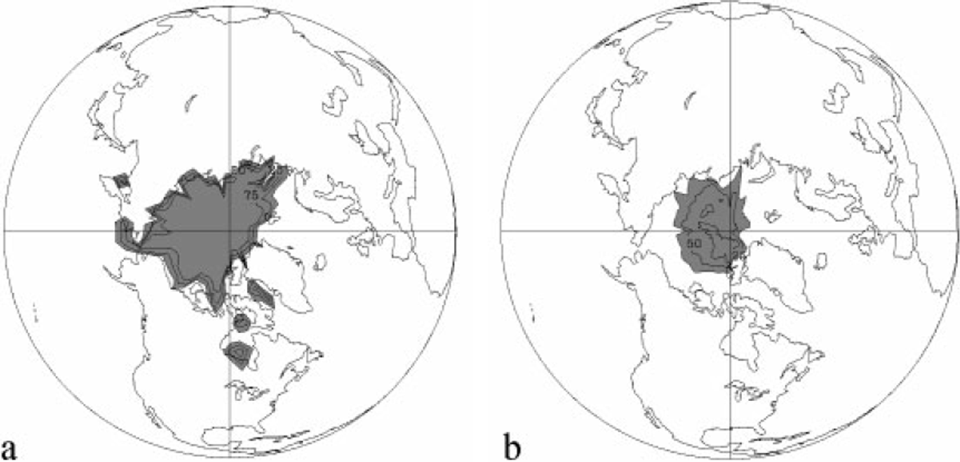
Fig. 6. Monthly mean ice concentration in august from (a) control and (b) co 2 experiments. shaded areas are concentrations of > 0.25.
Recent satellite-based observations show a decrease of Northern Hemisphere sea ice since 1978. Various groups of scientists had found from satellite observations and historical records of ice extent that the Arctic sea-ice cover has been shrinking at a rate of about 3% per decade during recent decades (Reference Maslanik, Serreze and BarryMaslanik and others, 1996; Reference Cavalieri, Parkinson, Gloersen, Comiso and ZwallyCavalieri and others, 1999; Reference Gloersen, Parkinson, Cavalieri, Comiso and ZwallyGloersen and others, 1999; Reference Johannessen, Shalina and MilesJohannessen and others, 1999; Reference Parkinson, Cavalieri, Gloersen, Zwally and ComisoParkinson and others, 1999; Reference Deser, Walsh and TimlinDeser and others, 2000). Figure 7 shows the Northern Hemisphere sea-ice-cover change based on linear trend from the satellite data (NSIDC, 1997) from 1979 to 1996. The analysis of satellite data shows a reduction of sea-ice cover every season, with maximum decrease in spring and summer. In summer, a decrease of sea-ice extent was observed in both the Eurasian and Canadian basins of the Arctic, while there is an increase of sea-ice extent north of Greenland and in Baffin Bay, which might be explained by enhancement of sea-ice transport in summer. This pattern of diminishing ice cover east of Greenland, and increasing ice cover west of Greenland, is similar to that reported by Reference Deser, Walsh and TimlinDeser and others (2000). The latest sea-ice extent data of the Hadley Centre for Climate Prediction and Research (Bracknell, U.K.) global sea-ice and SSTdataset (GISST 4.0) show a reduction of sea-ice cover from 1951 to 1998 during fall, winter and spring, with twice as large a reduction during summer. The simple mixed-layer Q.-flux model reveals a seasonality of sea-ice reduction in the Northern Hemisphere (Fig. 8) consistent with observational data. The summer decrease of sea cover is almost double that in winter and spring. In fall the model shows a residual high shrinkage of sea-ice cover, but this is smaller than in summer.

Fig. 7. Observed northern hemisphere sea-ice-cover change based on linear trend for 1979−96 (NSIDC, 1997): (a) december-february; (b) march-may; ( c) june-august; ( d) september-november.

Fig. 8. Northern hemisphere sea-ice-cover change (greenhouse experiment minus control), averaged over the last 20 years of simulations: (a) december-february; (b) march-may; ( c) june-august; (d) september-november.
Conclusion
We have investigated the interannual variability of the GISS Q-flux global climate model. This model uses a monthly-varying mixed-layer depth and specified horizontal heat transports. Natural climatic variability consists of multi-decadal warming and cooling periods, with the largest year-to year variations of sea ice in the marginal ice zone and the shelf seas. The overall behavior of the control Q-flux climate model is reasonably consistent with observations.
The sensitivity of a global climate model to an increase of the CO2 content in the atmosphere has considerable spatial and temporal variations. The CO2−induced warming of the surface air is large at high latitudes owing to the poleward retreat of snow cover and sea ice and more stable atmospheric lapse rates. Over the northern polar region, the warming of the surface atmospheric layer of the model is much larger in winter than in summer. The additional heat energy absorbed by the oceans during the warm season delays the appearance of the sea ice. This reduces the thermal insulation effect of the sea ice, enhancing the warming of the surface atmospheric layer.
The Northern Hemisphere sea-ice area from the control experiment is about 20% greater than the satellite values. The analysis of sea-ice thickness for the central Arctic shows that the control Q.-flux model produces a smaller seasonal cycle of ice thickness compared to observations (Reference Rothrock, Yu and MaykutRothrock and others, 1999). These problems are presumed to be mainly a result of the omission of sea-ice dynamics.
The experiment yields a reduction of sea-ice area and 55% thinning of ice in August in the Northern Hemisphere. The annual mean sea-ice shrinkage due to doubled CO2 is about 30% for the Northern Hemisphere. This is consistent with the results of Reference Pollard and ThompsonPollard and Thompson (1994), where they compare the response of dynamical and motionless sea ice to doubled CO2.
Seasonal variability of the Northern Hemisphere sea-ice cover is consistent with observational data. Both satellite data and the surface-based historical record of sea-ice extent show shrinkage of the Arctic sea-ice cover, with maximum decrease in summer. The greenhouse Q-flux model reveals the largest reduction of sea-ice extent in summer, which is almost double the winter decrease, with residual high shrinkage in fall.


