


1. Introduction
1.1. The broader context
The action of breaking waves on the ocean surface has a large and incompletely understood effect on the dynamics of mass, momentum and energy transfer between the ocean and the atmosphere, converting much of the wave energy into heat in a complex process that spans a wide range of scales (Melville Reference Melville1996). Breaking also marks a transition at the ocean surface from laminar flow to two-phase turbulent mixing at small scales, modulating the dynamics of the upper ocean sub-mesoscales, particularly via Langmuir turbulence and fronts (McWilliams Reference McWilliams2016), and affects the transport of particles with implications for the fate of oil spills and plastic pollutants (Deike, Pizzo & Melville Reference Deike, Pizzo and Melville2017; Pizzo, Melville & Deike Reference Pizzo, Melville and Deike2019). Furthermore, surface breaking injects a large amount of gas into the ocean via the entrainment of bubbles, including approximately  $30\,\%$ of the $\textrm {CO}_2$ that has been released into the atmosphere (Deike & Melville Reference Deike and Melville2018; Reichl & Deike Reference Reichl and Deike2020); breaking also ejects spray into the atmosphere, where it can convect and evaporate to leave salt crystals that may serve as cloud condensation nuclei (de Leeuw et al. Reference de Leeuw, Andreas, Anguelova, Fairall, Lewis, O'Dowd, Schulz and Schwartz2011; Veron Reference Veron2015).
Wave breaking involves transition from two-dimensional (2-D) laminar wave flow to three-dimensional (3-D) turbulence. As wave energy focuses through linear or nonlinear processes, local conditions on a wave surface become unstable and cause breaking, which transfers energy and momentum to the water column. The geometry and kinematics of the breaking waves have been studied extensively (Longuet-Higgins & Cokelet Reference Longuet-Higgins and Cokelet1976; Perlin, Choi & Tian Reference Perlin, Choi and Tian2013; Schwendeman & Thomson Reference Schwendeman and Thomson2017; Fedele, Banner & Barthelemy Reference Fedele, Banner and Barthelemy2020), and the identification of a breaking threshold with approaches based on the wave kinematics, dynamics or geometry remains a longstanding issue (Melville Reference Melville1982; Banner & Peirson Reference Banner and Peirson2007; Perlin et al. Reference Perlin, Choi and Tian2013), with recent work discussing the link between the breaker kinematics and dynamics (Saket et al. Reference Saket, Peirson, Banner, Barthelemy and Allis2017; Derakhti et al. Reference Derakhti, Kirby, Banner, Grilli and Thomson2020; Pizzo Reference Pizzo2020).
While the initiation of the breaking phenomenon and the turbulence generated by it have been characterized (Rapp & Melville Reference Rapp and Melville1990; Duncan, Qiao & Philomin Reference Duncan, Qiao and Philomin1999; Tulin & Waseda Reference Tulin and Waseda1999; Melville, Veron & White Reference Melville, Veron and White2002; Banner & Peirson Reference Banner and Peirson2007; Drazen, Melville & Lenain Reference Drazen, Melville and Lenain2008; Drazen & Melville Reference Drazen and Melville2009), the time and length scales of the transition process remain to be explored. During this transition to turbulence, air is entrained, and bubbles are formed (Lamarre & Melville Reference Lamarre and Melville1991; Deane & Stokes Reference Deane and Stokes2002) and spray droplets are ejected (Erinin et al. Reference Erinin, Wang, Liu, Towle, Liu and Duncan2019). The measurement of 3-D two-phase turbulence in the laboratory and in the field presents many technical challenges in terms of accessing successfully the turbulent flow field and the size distributions of drops and bubbles during the active time of breaking.
Direct numerical simulations (DNS) therefore appear as an appealing tool. Owing to the computational difficulty and expense of modelling 3-D multiphase flows, numerical studies began by using 2-D breakers as analogues for the full 3-D processes (Chen et al. Reference Chen, Kharif, Zaleski and Li1999; Song & Sirviente Reference Song and Sirviente2004; Iafrati Reference Iafrati2009, Reference Iafrati2011; Deike, Popinet & Melville Reference Deike, Popinet and Melville2015). Early development of nonlinear potential flow models has shed light on the breaking process up to the moment of impact (Longuet-Higgins & Cokelet Reference Longuet-Higgins and Cokelet1976; Dommermuth et al. Reference Dommermuth, Yue, Lin, Rapp, Chan and Melville1988), while 3-D simulations have used reduced models such as large-eddy simulations (LES) to capture the breaking process itself (Watanabe, Saeki & Hosking Reference Watanabe, Saeki and Hosking2005; Lubin & Glockner Reference Lubin and Glockner2015; Hao & Shen Reference Hao and Shen2019), but the complete resolution of the breaker in DNS in three dimensions has only recently become feasible (Fuster et al. Reference Fuster, Agbaglah, Josserand, Popinet and Zaleski2009; Deike, Melville & Popinet Reference Deike, Melville and Popinet2016; Wang, Yang & Stern Reference Wang, Yang and Stern2016; Yang, Deng & Shen Reference Yang, Deng and Shen2018). Surprisingly, despite the essentially 3-D nature of the turbulence resulting from breaking, 2-D breakers at the tested conditions have provided a reasonable estimate of the dissipation rates obtained from experiments and 3-D computation (discussed further below). In contrast, the turbulent dissipation in internal wave breaking has been shown to be a clear 3-D process (Gayen & Sarkar Reference Gayen and Sarkar2010).
1.2. Laboratory experiments and direct numerical simulations of canonical breaking waves
Canonical breaking waves have been studied using a variety of different approaches, both experimental and numerical (Duncan Reference Duncan1981; Melville Reference Melville1982, Reference Melville1994; Rapp & Melville Reference Rapp and Melville1990; Duncan et al. Reference Duncan, Qiao and Philomin1999; Banner & Peirson Reference Banner and Peirson2007; Drazen et al. Reference Drazen, Melville and Lenain2008; Tian, Perlin & Choi Reference Tian, Perlin and Choi2010; Erinin et al. Reference Erinin, Wang, Liu, Towle, Liu and Duncan2019). Studies such as these have identified the main controlling parameters of breaking waves, namely the breaking speed and the wave slope at breaking  $S=ak$, where $a$ is the wave amplitude, and $k$ is the wavenumber. The bandwidth of the wave packet is also important, and the detailed kinematics before breaking, in particular a significant slowdown of the wave crest, have been discussed in order to propose breaking threshold criteria (Banner et al. Reference Banner, Barthelemy, Fedele, Allis, Benetazzo, Dias and Peirson2014; Saket et al. Reference Saket, Peirson, Banner, Barthelemy and Allis2017; Pizzo & Melville Reference Pizzo and Melville2019; Derakhti et al. Reference Derakhti, Kirby, Banner, Grilli and Thomson2020; Fedele et al. Reference Fedele, Banner and Barthelemy2020), although we will neglect its influence from here onwards.
It follows that DNS of breaking waves can be framed in terms of a set of non-dimensional numbers. The relevant parameters are the air–water density and viscosity ratios, the wave speed and wavenumber, and amplitude. These define a wave Reynolds number and the wave slope as
 \begin{equation} {Re} = \frac{\sqrt{g\lambda_0^3}}{\nu}, \quad S = ak, \end{equation}
where  $\lambda _0 = 2{\rm \pi} /k$ is the wavelength and $\nu$ is the kinematic viscosity of the water. Similarly to turbulent DNS, numerical simulations of breaking waves are confined typically to the highest $Re$ accessible to available computation effort, which has grown over time. Iafrati (Reference Iafrati2009), Deike et al. (Reference Deike, Popinet and Melville2015, Reference Deike, Melville and Popinet2016) and De Vita, Verzicco & Iafrati (Reference De Vita, Verzicco and Iafrati2018) have typically used $Re=40\times 10^3$.
To consider bubble and droplet generation, the Bond number is needed:
 \begin{equation} {Bo} = \frac{{\rm \Delta} \rho\,g}{\sigma k^2}, \end{equation}
where  ${\rm \Delta} \rho$ is the density difference between air and water, and $\sigma$ is the surface tension. The Bond number $Bo$ corresponds to the ratio between the wavelength and the capillary length scale.
Deike et al. (Reference Deike, Popinet and Melville2015, Reference Deike, Melville and Popinet2016) used the Bond number to compare the numerical wavelength to experimental results. Deike et al. (Reference Deike, Popinet and Melville2015) describes the wave patterns for a large range of  $Bo$ and $S$, discussing the energetics of parasitic capillary waves, spilling breakers and plunging breakers. As discussed in Iafrati (Reference Iafrati2009) and Deike et al. (Reference Deike, Popinet and Melville2015, Reference Deike, Melville and Popinet2016), the breaking waves in a laboratory would approach $Re=10^6$. Despite this difference in $Re$, DNS (Iafrati Reference Iafrati2009; Deike et al. Reference Deike, Popinet and Melville2015, Reference Deike, Melville and Popinet2016) and LES (Derakhti & Kirby Reference Derakhti and Kirby2014, Reference Derakhti and Kirby2016) found good agreement between experiments and simulations for the non-dimensional energy dissipation due to breaking as a function of the breaker slope (see figure 1). Nevertheless, an outstanding challenge in DNS is the correct numerical resolution of processes whose separation of scales increases with $Re$ and $Bo$. For such simulations to capture the physics of breaking waves correctly, they must resolve all scales between and including those of energy dissipation and the formation and breakup of bubbles and droplets in a two-phase turbulent environment. This requires capturing the full physics of the problem, while retaining a qualitatively faithful representation of the breaking process in comparison with experiment. Historically, these very difficult challenges have limited the scope of DNS investigations, the details of whose approaches are discussed in more detail below.

Figure 1. Breaking parameter  $b$ as a function of wave slope $S$. Red cross indicates present DNS data. Inverted red triangles indicate DNS data from Deike et al. (Reference Deike, Melville and Popinet2016). Black and grey indicate experimental data due to Drazen et al. (Reference Drazen, Melville and Lenain2008), Banner & Peirson (Reference Banner and Peirson2007) and Grare et al. (Reference Grare, Peirson, Branger, Walker, Giovanangeli and Makin2013). Solid line is $b=0.4(S-0.08)^{5/2}$, a semi-empirical result of Romero et al. (Reference Romero, Melville and Kleiss2012). Shaded area indicates the uncertainties on the scaling for $b$.
$b$.
Both the wave Reynolds number and the Bond number characterize the overall scale of the wave through its wavelength and phase speed, compared with viscous and capillary effects. Once the wave breaks, the turbulence that it generates is controlled by the breaking slope together with the speed of the breaker, and is itself characterized by a turbulent Reynolds number, defined typically using the Taylor micro-scale  $Re_{\lambda }$, with Drazen & Melville (Reference Drazen and Melville2009) typically finding values around $Re_{\lambda }\simeq 500$. Similarly, the fragmentation processes and generation of drops and bubbles in a turbulent flow are usually analysed in terms of a Weber number, comparing the inertial stresses due to the turbulence to the surface tension.
1.3. Energetics and dimensionality of breaking waves
Breaking waves dissipate energy, generating a turbulent two-phase flow with properties that can be related to the local breaking properties (Duncan Reference Duncan1981). The local turbulent dissipation rate due to breaking can be described by an inertial scaling (Drazen et al. Reference Drazen, Melville and Lenain2008)
 \begin{equation} \varepsilon=(\sqrt{gh})^3/h, \end{equation}
where  $h$ is the breaking height, here consistently defined as half the distance between wave crest and trough, and $\sqrt {gh}$ the ballistic velocity of the plunging breaker, with $g$ the acceleration due to gravity. The turbulence is confined to a volume $\mathcal {V}_0=AL_c$, of cross-section that is generally assumed to be $A\simeq {\rm \pi}h^2/4$ (Duncan Reference Duncan1981; Drazen et al. Reference Drazen, Melville and Lenain2008), and length of breaking crest $L_c$, leading to an integrated dissipation rate per unit length of breaking crest given by
 \begin{equation} \epsilon_l = \rho A \varepsilon. \end{equation}
This scaling can be related to the initial slope, bandwidth and speed of the wave packet in controlled laboratory experiments (Duncan Reference Duncan1981; Rapp & Melville Reference Rapp and Melville1990; Banner & Peirson Reference Banner and Peirson2007; Drazen et al. Reference Drazen, Melville and Lenain2008; Tian et al. Reference Tian, Perlin and Choi2010; Grare et al. Reference Grare, Peirson, Branger, Walker, Giovanangeli and Makin2013) and numerical simulations (Iafrati Reference Iafrati2009; Deike et al. Reference Deike, Popinet and Melville2015, Reference Deike, Melville and Popinet2016; Derakhti & Kirby Reference Derakhti and Kirby2016). The breaking parameter  $b$ is a non-dimensional measure of the dissipation that was introduced by Duncan (Reference Duncan1981) and Phillips (Reference Phillips1985), and relates to $\epsilon _l$ as
 \begin{equation} \epsilon_l=b\rho c^5/g, \end{equation}
which combined with the local dissipation rate argument above, and assuming that the breaking speed is related to the wavenumber by the dispersion relation  $c = \sqrt {g/k}$, leads to $b \propto S^{5/2}$ (Drazen et al. Reference Drazen, Melville and Lenain2008). Introducing a slope-based breaking threshold $S_0$, this formulation for the breaking parameter reads
 \begin{equation} b=\chi_0(S-S_0)^{5/2}. \end{equation}
Extensive laboratory experiments have demonstrated the accuracy of the physics-based model, with  $\chi _0\simeq 0.4$ and $S_0\simeq 0.08$ used as fitting parameters by Romero, Melville & Kleiss (Reference Romero, Melville and Kleiss2012), allowing us to account for numerous laboratory data (Duncan Reference Duncan1981; Rapp & Melville Reference Rapp and Melville1990; Banner & Peirson Reference Banner and Peirson2007; Drazen et al. Reference Drazen, Melville and Lenain2008; Tian et al. Reference Tian, Perlin and Choi2010; Grare et al. Reference Grare, Peirson, Branger, Walker, Giovanangeli and Makin2013). Several numerical studies have confirmed this scaling and validated their approaches against this result (Derakhti & Kirby Reference Derakhti and Kirby2014, Reference Derakhti and Kirby2016; Deike et al. Reference Deike, Popinet and Melville2015, Reference Deike, Melville and Popinet2016, Reference Deike, Pizzo and Melville2017; De Vita et al. Reference De Vita, Verzicco and Iafrati2018). Figure 1 shows $b$ as a function of $S$ for a variety of experimental and numerical data, including from the present study. We note that experimental work using the linear focusing technique typically considers the linearly predicted wave slope, summed over all components, while numerical work using compact wave initialization has considered the initial slope. In all cases, the slope being used is proportional to the breaking slope, as discussed in Drazen et al. (Reference Drazen, Melville and Lenain2008) for experimental data and Deike et al. (Reference Deike, Popinet and Melville2015, Reference Deike, Melville and Popinet2016) for numerical data, which allows comparison between the experimental and numerical work. The differences in definitions and estimations may therefore be responsible for some of the scatter in figure 1 between the various data sets, and uncertainties in the fitting coefficients are indicated by the shaded area. Note that the scaling $b\propto S^{5/2}$ is observed at high slopes for both the experiments and DNS. Moreover, the proportion of energy dissipated by breaking for a given slope is similar between experiments and simulations. This fundamental model for the turbulent dissipation rate has been used successfully as the physical basis of larger-scale spectral wave models (Romero et al. Reference Romero, Melville and Kleiss2012; Romero Reference Romero2019). Moreover, we proposed recently an extension of the inertial argument to certain types of shallow water breakers (Mostert & Deike Reference Mostert and Deike2020).
It remains to determine the particular transition characteristics of the fully 3-D flow, and to investigate the dependence of these characteristics on the flow Reynolds number, as well as on the evolution of the ingested bubble plume. Furthermore, even aside from limitations on the maximum values of  $Re,Bo$ attainable in computation, many numerical studies have investigated 2-D breakers as computationally feasible analogues for the full 3-D processes (Song & Sirviente Reference Song and Sirviente2004; Hendrickson & Yue Reference Hendrickson and Yue2006; Iafrati Reference Iafrati2009; Deike et al. Reference Deike, Popinet and Melville2015). Surprisingly, despite the essentially 3-D nature of the turbulence resulting from the breaking process, 2-D breakers at the tested conditions provided a reasonable estimate of the dissipation rates for 3-D breakers obtained from computation and experiment, with discrepancies sometimes as small as $5\,\%$ (Lubin et al. Reference Lubin, Vincent, Abadie and Caltagirone2006; Iafrati Reference Iafrati2009). Favourable comparison with semi-empirical models as discussed above also suggests the usefulness of 2-D computations for the dissipation rate (Deike et al. Reference Deike, Popinet and Melville2015). Nonetheless, the details of the 2-D/3-D transition physics in breaking waves constitute an open question. The present study will go some way to addressing these questions, with suggestion of a possible transition to turbulence with an associated turbulent Reynolds number.
1.4. Bubble size distributions in breaking waves
A breaking wave entrains air, which is characterized by a broad size distribution of bubbles. Direct investigation of the bubble distribution, obviously not available within a 2-D study, is important to inform subgrid scale models used in LES (Shi, Kirby & Ma Reference Shi, Kirby and Ma2010; Liang et al. Reference Liang, McWilliams, Sullivan and Baschek2011, Reference Liang, McWilliams, Sullivan and Baschek2012; Derakhti & Kirby Reference Derakhti and Kirby2014) and gas transfer models (Liang et al. Reference Liang, McWilliams, Sullivan and Baschek2011; Deike & Melville Reference Deike and Melville2018). Garrett, Li & Farmer (Reference Garrett, Li and Farmer2000) proposed a turbulent breakup cascade model for the size distribution per unit volume  $\mathcal {N}(r)$, where $r$ is the bubble radius, as a function of the local dissipation rate $\bar {\varepsilon }$ with constant volumetric air flow rate $Q$, with a dimensional analysis yielding
 \begin{equation} \mathcal{N}(r) \propto Q \bar{\varepsilon}^{{-}1/3} r^{{-}10/3}. \end{equation}
We note that a time-averaged dissipation rate  $\bar {\varepsilon }$ over the breaking time has been considered when analysing and scaling various data sets in Deane & Stokes (Reference Deane and Stokes2002) and Deike et al. (Reference Deike, Melville and Popinet2016). The corresponding breakup model assumes a turbulent inertial subrange with a direct cascade, with large bubbles injected at one end of the cascade by a notional entrainment process, and turbulent fluctuations then breaking these into smaller bubbles. The lower end of the cascade is set by the Hinze scale (Hinze Reference Hinze1955; Deane & Stokes Reference Deane and Stokes2002; Perrard et al. Reference Perrard, Rivière, Mostert and Deike2021)
 \begin{equation} r_H = \mathcal{C}_0 \left( \frac{\sigma}{\rho}\right)^{3/5} \bar{\varepsilon}^{{-}2/5}. \end{equation}
Here,  $\mathcal {C}_0\simeq 0.4$ (Deane & Stokes Reference Deane and Stokes2002) is a dimensionless constant. Its value is related to the critical Weber number defining bubble breakup, which ranges typically from 1 to 5 (Risso & Fabre Reference Risso and Fabre1998; Martinez-Bazan, Montanes & Lasheras Reference Martinez-Bazan, Montanes and Lasheras1999; Deane & Stokes Reference Deane and Stokes2002; Vejražka, Zedníková & Stanovskỳ Reference Vejražka, Zedníková and Stanovskỳ2018; Perrard et al. Reference Perrard, Rivière, Mostert and Deike2021; Rivière et al. Reference Rivière, Mostert, Perrard and Deike2021), with estimations of $\mathcal {C}_0$ varying by about a factor of 2. These differences are related to variations in the experimental protocols and the large-scale structure of the turbulent flow. Note also that the breaking wave problem is transient in nature, so that the Hinze scale might present variations in time, and estimations of the Hinze scale based on the averaged turbulence dissipation rate present an added uncertainty. For all these reasons, it should be considered a soft limit. The size distribution below the Hinze scale is not addressed by Garrett et al. (Reference Garrett, Li and Farmer2000).
Laboratory experiments have reported measurements of the bubble size distribution under a breaking wave using various optical and acoustic techniques (Loewen, O'Dor & Skafel Reference Loewen, O'Dor and Skafel1996; Terrill, Melville & Stramski Reference Terrill, Melville and Stramski2001; Deane & Stokes Reference Deane and Stokes2002; Leifer & de Leeuw Reference Leifer and de Leeuw2006; Rojas & Loewen Reference Rojas and Loewen2007; Blenkinsopp & Chaplin Reference Blenkinsopp and Chaplin2010), in general agreement with the model from Garrett et al. (Reference Garrett, Li and Farmer2000). Theoretical and numerical investigation has further strengthened understanding of the turbulent bubble cascade above the Hinze scale (Chan, Johnson & Moin Reference Chan, Johnson and Moin2020a,Reference Chan, Johnson and Moinb). Deike et al. (Reference Deike, Melville and Popinet2016) demonstrated the ability of numerical methods to reproduce the size distribution observed experimentally and described theoretically, with an extension of the theory to constrain the mean air flow rate for increasing wave slopes. That study also noted a correspondence between the development of the entrained bubble population and the wave's energy dissipation rate. For bubbles below the Hinze scale, however, there is significant scatter between existing data sets, although Deane & Stokes (Reference Deane and Stokes2002) suggests a relationship  $\propto r^{-3/2}$.
The numerical studies from Deike et al. (Reference Deike, Melville and Popinet2016) and Wang et al. (Reference Wang, Yang and Stern2016) had limited resolution of sub-Hinze-scale bubbles and were performed at  $Re=40\times 10^3$, $Bo=200$, with the assumption that the bubble size distributions were independent of $Re$ and $Bo$, like the dissipation rate (see § 1.3). The present DNS study brings to bear sophisticated methods and computational resources to test the dependence on $Re,Bo$ of the bubble size distribution, and to resolve the sub-Hinze bubble statistics. These constitute two of the main objectives of the present study.
1.5. Droplet size distributions in breaking waves
The mechanisms of spray generation by breaking waves have been reviewed recently by Veron (Reference Veron2015). Droplet size distributions have been explored experimentally in the presence of wind (Wu Reference Wu1979; Veron et al. Reference Veron, Hopkins, Harrison and Mueller2012; Ortiz-Suslow et al. Reference Ortiz-Suslow, Haus, Mehta and Laxague2016; Troitskaya et al. Reference Troitskaya, Kandaurov, Ermakova, Kozlov, Sergeev and Zilitinkevich2018) as well as for deep water breaking waves generated by linear focusing (Erinin et al. Reference Erinin, Wang, Liu, Towle, Liu and Duncan2019), while numerical investigations have been made of Lagrangian transport of spume droplets in the air (Richter & Sullivan Reference Richter and Sullivan2013; Druzhinin, Troitskaya & Zilitinkevich Reference Druzhinin, Troitskaya and Zilitinkevich2017; Tang et al. Reference Tang, Yang, Liu, Dong and Shen2017). However, a general theoretical model for the droplet size distribution has not been formulated.
In the context of breaking waves, spray is not created in the same manner as bubbles in the flow, being instead more analogous to atomization and fragmentation droplets (Veron et al. Reference Veron, Hopkins, Harrison and Mueller2012; Troitskaya et al. Reference Troitskaya, Kandaurov, Ermakova, Kozlov, Sergeev and Zilitinkevich2018; Villermaux Reference Villermaux2020). They are generated by two main mechanisms: direct ejection from wave impact and the related dynamic interface evolution, and indirect jet ejection resulting from the bursting of bubbles that were entrained initially by the breaker (Lhuissier & Villermaux Reference Lhuissier and Villermaux2012; Deike et al. Reference Deike, Ghabache, Liger-Belair, Das, Zaleski, Popinet and Seon2018; Berny et al. Reference Berny, Deike, Séon and Popinet2020). The latter population is typically much smaller than the former (Veron Reference Veron2015), hence even more challenging to resolve numerically within the breaking wave event, but can be studied separately (Deike et al. Reference Deike, Ghabache, Liger-Belair, Das, Zaleski, Popinet and Seon2018; Berny et al. Reference Berny, Deike, Séon and Popinet2020). Separately, a major complicating factor is that spray droplet populations are typically significantly smaller than bubble populations for a given breaking wave, leading to challenges in statistical convergence of the data. For these reasons, experimental and numerical studies of droplet production by breaking waves are limited (Wang et al. Reference Wang, Yang and Stern2016; Erinin et al. Reference Erinin, Wang, Liu, Towle, Liu and Duncan2019). In this study, droplet populations are resolved over a sufficient range of length scales to allow comparison with experiment, showing good agreement in the shape of the resolved size distribution. Velocity and joint velocity–size distributions are also shown, which will aid future studies.
1.6. Outline
In this paper, we present high-resolution DNS, which mobilizes sophisticated tools and computational resources to advance the following challenges: we will show statistics spanning multiple scales of fluid behaviour for full 3-D simulations that capture breaking physics as seen in laboratory experiments regarding energy dissipation, bubble and droplets size distribution. The set-up is similar to Deike et al. (Reference Deike, Melville and Popinet2016) and is analogous to deep water breaking waves in the laboratory obtained by focusing packets (Deane & Stokes Reference Deane and Stokes2002; Drazen et al. Reference Drazen, Melville and Lenain2008), as demonstrated by Deike et al. (Reference Deike, Melville and Popinet2016), but increased resolution of the interfacial processes allows access to higher Reynolds and Bond numbers to describe the transition to 3-D turbulence, and the formation of droplets and bubbles down to scales comparable to state-of-the-art laboratory experiments. These simulations represent the current state of the art in multiphase simulations of breaking waves and further confirm that the physics of breaking waves can be investigated profitably through these high-fidelity numerical data. We analyse the role of these parameters in interfacial processes, including air entrainment, bubble statistics and droplet statistics. We discuss how energy dissipation, bubble and droplet statistics seem independent of the Reynolds number above a certain value, for the strong plunging breakers, confirming the results obtained previously at lower Reynolds numbers by comparison with experimental data. Next, we investigate the role of the capillary length and other flow scales on the air entrainment and spray production, which are most likely to mediate the development of transverse instabilities in the breaking process. We emphasize that such a study is possible only thanks to improvement in adaptive mesh refinement (AMR) techniques, along with increasing computational power, which has enabled sufficiently high resolution.
The paper proceeds as follows. In § 2, we describe the numerical methods and the formulation of the physical problem, the transition from the initial planar configuration to fully-developed 3-D flows, and the general processes that produce entrained bubbles and ejected spray. In § 3, we investigate the development of the 3-D flow in direct comparisons with 2-D computations, as well as the role of transverse instabilities and their influence on the dissipation rate. We study the transition time and length scale of the breaking flow, from its initial 2-D configuration, to the final 3-D turbulent one. Then, in § 4, we present a bubble size distribution at higher  $Re, Bo$ and numerical resolutions than those found in the numerical literature, and extend below the Hinze scale at lower $Re, Bo$. Droplet size and velocity distributions are presented in § 5, before we conclude in § 6.
2. Problem formulation and numerical method
2.1. Basilisk library
We use the Basilisk library to solve the two-phase incompressible Navier–Stokes equations with surface tension, in two and three dimensions. The successor of the Gerris flow solver (Popinet Reference Popinet2003, Reference Popinet2009), Basilisk is able to solve a diversity of partial differential equation systems in an AMR framework that decreases significantly the cost of high-resolution computations, allowing an efficient representation of multiscale processes. Flow advection is approximated using the Bell–Colella–Glaz method (Bell, Colella & Glaz Reference Bell, Colella and Glaz1989), and the viscous terms are solved implicitly. The interface between distinct gas and liquid is described by a geometric volume-of-fluid (VOF) advection scheme, with a well-balanced surface tension treatment that mitigates the generation of parasitic currents (Popinet Reference Popinet2018). A momentum-conserving implementation allows us to avoid artefacts due to momentum ‘leaking’ between the dense and light phases (Fuster & Popinet Reference Fuster and Popinet2018; Zhang, Popinet & Ling Reference Zhang, Popinet and Ling2020). The governing equations can be written as
 \begin{gather} \frac{\partial \rho}{\partial t} + \boldsymbol{\nabla}\boldsymbol{\cdot}\left(\rho\boldsymbol{u} \right) = 0, \end{gather}
 \begin{gather}\rho \left( \frac{\partial \boldsymbol{u}}{\partial t } + \boldsymbol{u} \boldsymbol{\cdot} \boldsymbol{\nabla} \boldsymbol{u} \right) ={-}\boldsymbol{\nabla} p + \boldsymbol{\nabla} \boldsymbol{\cdot} (2\mu \boldsymbol{D}) + \rho\boldsymbol{g} + \sigma \kappa \delta_s \boldsymbol{n}, \end{gather}
 \begin{gather}\boldsymbol{\nabla} \boldsymbol{\cdot} \boldsymbol{u} = 0, \end{gather}
where  $\rho, \boldsymbol {u}, \mu, \sigma, \boldsymbol {D}, \boldsymbol {g}$ are the fluid density, velocity vector, dynamic viscosity, surface tension, deformation tensor and gravitational acceleration vector, respectively. The density and viscosity are allowed to vary according to a volume fraction field $c(\boldsymbol {x}, t)$ that in these simulations takes the value zero in the gas phase and unity in the liquid phase. The variable $\delta _s$ is a Dirac delta that concentrates surface tension effects into the liquid–gas interface; $\kappa$ is the curvature of the interface, and $\boldsymbol {n}$ is its unit normal vector.
2.2. Wave initialization
We consider breaking waves in deep water. The relevant physical parameters are the liquid and gas  $\rho _w, \rho _a$, respectively, the respective dynamic viscosities $\mu _w, \mu _a$, the surface tension $\sigma$, the wavelength $\lambda _0$, initial wave amplitude $a$, and gravitational acceleration $g$. The water depth $h_0$, while finite, is assumed sufficiently large so that it does not affect significantly the breaking physics. The eight significant parameters, which are expressed in three physical dimensions, can thus be reduced into five dimensionless groups according to Buckingham's theorem; these are the density ratio $\rho _a/\rho _w$, viscosity ratio $\mu _a/\mu _w$, wave slope $S = a k$, where $k=2{\rm \pi} /\lambda _0$ is the wavenumber, and the Bond and Reynolds numbers as defined previously, ${Bo} = {\rm \Delta} \rho \,g/\sigma k^2$, ${Re} = \sqrt {g\lambda _0^3}/\nu _w$, where ${\rm \Delta} \rho = \rho _w - \rho _a \simeq \rho _w$, and $\nu _w = \mu _w/\rho _w$ is the kinematic viscosity. The wave period is $T = \lambda _0/c = 2{\rm \pi} /\sqrt {gk}$, where $c=\sqrt {g/k}$ is the linear phase speed for deep water gravity waves. The governing equations (2.1)–(2.3) can be non-dimensionalized in terms of these groups. These definitions follow the literature; see Chen et al. (Reference Chen, Kharif, Zaleski and Li1999), Iafrati (Reference Iafrati2009) and Deike et al. (Reference Deike, Popinet and Melville2015, Reference Deike, Melville and Popinet2016).
The numerical resolution is indicated by the smallest cell size attained in the simulation, given by  $\Delta = \lambda _0/2^L$, where $L$ is the maximum level of refinement used in the AMR scheme. The refinement criterion is based on both the velocity field and the VOF tracer field. The maximum resolution used in this study is $L=11$, corresponding to a conventional grid of $(2^{11})^3$, or approximately 8.6 billion, total cells. Under the AMR scheme, the grid size reduces to the order of 150 million cells at $L=11$.
We initialize the breaking wave following Chen et al. (Reference Chen, Kharif, Zaleski and Li1999), Iafrati (Reference Iafrati2011), Deike et al. (Reference Deike, Popinet and Melville2015, Reference Deike, Melville and Popinet2016), Wang et al. (Reference Wang, Yang and Stern2016) and Chan et al. (Reference Chan, Johnson and Moin2020a,Reference Chan, Johnson and Moinb), based on an unstable third-order Stokes wave for the water velocity and zero velocity in the air. The flow is regularized in the first time step. We note that the Stokes wave solution has been derived for an irrotational inviscid free surface wave, hence remains an imperfect initial condition for the full two-phase flow problem, accounting for viscosity and surface tension. However, numerous studies have demonstrated that it provides an efficient and compact initialization to study the post-breaking processes. Both 2-D and 3-D simulations are conducted in order to investigate the transition from the laminar, planar and essentially 2-D initial evolution to the final, turbulent, 3-D flow. Besides the dimensional difference, the 2-D simulations are initialized identically to the 3-D simulations. In the 3-D simulations, no perturbation is used to seed the transition from planar to non-planar evolution of the wave; this transition is brought about by numerical noise during the breaking process.
2.3. Parameter space
The density and viscosity ratios are fixed to the values for water and air,  $\rho _w/\rho _a = 850$, $\mu _w/\mu _a = 51.15$, and the input slope is fixed at a nominal value $S=0.55$, leaving the remaining two groups, $Re, Bo$ to be varied. Thus we investigate the independent effects of variation in surface tension through $Bo$, and viscosity through $Re$. The fixed value of $S$ is chosen to be sufficiently large to force the wave into a plunging breaker (Deike et al. Reference Deike, Popinet and Melville2015). We refer the reader to (Deike et al. Reference Deike, Melville and Popinet2016) for an extensive study on the role of the wave slope $S$ at constant $Re,Bo$. The parameters are shown in table 1, and correspond to low ( $Bo=200$), medium ( $Bo=500$) and high ( $Bo=1000$) Bond numbers, and low ( $Re=40\ 000$) and high ( $Re=100\ 000$) Reynolds numbers. Cases run to test grid convergence span moderate ( $L=10$) and fine ( $L=11$) resolutions, respectively. Some additional cases at a variety of Reynolds numbers are also run for the energetics comparison in § 3. We reach a maximum separation of defined scales (wavelength to Hinze scale) of a factor ${\sim }550$. The grid size for the $L=11$ case reaches 181 million cells, for a maximum runtime (excluding scheduling and queueing times) of 1.4 months and a cost of half a million CPU-hours. These highest resolution cases were run on the Stampede2 cluster at the Texas Advanced Computing Center of the University of Texas, typically on between 192 and 768 cores of the Skylake node system. (Portions of these simulations were also run on the high-performance computing resources of the French National Computing Center for Higher Education (CINES).) Lower-resolution cases ( $L=10$) were run on the TigerCPU cluster at Princeton University using typically between 160 and 320 cores. Note that while these simulations are expensive, they still save several orders of magnitude over a uniform- or fixed-grid approach, which would require a prohibitively large grid size of 8.6 billion cells in the highest-resolution case.
Table 1. Computational matrix of parameter space for 3-D breaking waves. The slope for each case is  $S=0.63$, modelling a strong plunging breaker. The column labels are as follows: $Re$, Reynolds number; $Bo$, Bond number; $L$, maximum level of grid refinement; $\lambda _0/r_H$, ratio of wavelength to Hinze scale; $\Delta /r_H$, ratio of smallest grid size to Hinze scale; $\Delta /l_c$, ratio of smallest grid size to the capillary length, defined as $l_c^2 = 1/(k^2Bo)$, where $k=2{\rm \pi} /\lambda _0$ is the wavenumber; $r_H/l_c$, ratio of Hinze scale to capillary length.

2.4. General flow characteristics
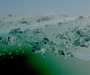
The wave evolves in a manner similar to that seen in previous studies with similar initialization (Deike et al. Reference Deike, Popinet and Melville2015, Reference Deike, Melville and Popinet2016). Figure 2 shows a sequence of stills at different stages of the breaking process. The initially planar wave steepens nonlinearly to a point where it locally develops a vertical interface (figures 2a,b). The wave then overturns, forming a jet that projects forwards into the upstream water surface (figure 2c), and impacts onto it (figure 2d), breaking the initially planar symmetry. At this moment, a large tube of air is ingested into the liquid bulk, which we refer to as the main cavity. The wave now also forms a fine-scale 3-D structure at the point of impact, while ingesting the tubular cavity. This cavity persists for some time until it breaks along its length into an array of large bubbles (at  $t/T=1\unicode{x2013}1.2$; figures 2e,f). In the meantime, the continuing breaking process on the surface creates a splash-up jet, as the wave proceeds into the strongly dissipative phase of the active breaking process (figure 2f) and develops into a fully developed 3-D flow (figures 2g,h) from $t/T=1.4$ onwards. At late times, most of the wave energy has been dissipated in the breaking process, but the turbulent regions persist for some time, during which a very large array of spray and especially bubbles is formed (figures 2f–h). All the presented cases produce a large quantity of bubbles of various sizes, but spray is produced abundantly, particularly at higher Bond numbers.

Figure 2. Snapshot renderings of the 3-D breaking wave water–air interface at different times, for the case  $Bo=500$, $Re=100\times 10^3$, at resolution $L=11$. (a) For $t/T=0.37$, nonlinear steepening and initial overturning. (b) For $t/T=0.56$, jet formation. (c,d) For $t/T=0.67, 0.8$, impact and ingestion of main cavity. (e) For $t/T=1.04$, splash-up of main wave and rupture of main cavity. (f–h) For $t/T=1.2, 1.36, 1.52$, continuation and slowdown of main breaking process.
These qualitative aspects of the breaking wave dynamics are crucial for a faithful representation of the breaking process. In this respect, the evolution and dynamics of the breaker resemble closely those of laboratory experiments, notwithstanding certain Bond and Reynolds number influences, and despite the different initializations across studies. The overturning phenomenon is very similar to that seen in Bonmarin (Reference Bonmarin1989), Rapp & Melville (Reference Rapp and Melville1990) and Drazen et al. (Reference Drazen, Melville and Lenain2008); the size and shape of the main ingested cavity matches very closely that seen in a large array of theoretical, numerical and experimental studies (Longuet-Higgins Reference Longuet-Higgins1982; New Reference New1983; New, McIver & Peregrine Reference New, McIver and Peregrine1985; Dommermuth et al. Reference Dommermuth, Yue, Lin, Rapp, Chan and Melville1988; Bonmarin Reference Bonmarin1989); and the subsequent droplet-producing splash sequence mirrors closely that seen in Erinin et al. (Reference Erinin, Wang, Liu, Towle, Liu and Duncan2019) (see § 5). This accurate reproduction of the breaker will be reflected further in various quantitative statistical comparisons with theory and experiment in the remainder of this paper, and moreover builds high confidence in the validity of our new results.
3. Energetics and transition to 3-D turbulent flow
We determine the effect of  ${Re}$ (and ${Bo}$) on the development of the 3-D turbulent flow underneath the breaking wave by direct comparisons of the 3-D simulations with 2-D counterparts.
3.1. Energy dissipation by breaking
The wave mechanical energy is  $E=E_P + E_K$, where $E_P = \int _V \rho g (z-z_0) \, {\rm d} V$ is the gravitational potential energy, with a gauge $z_0$ chosen such that $E_P=0$ for the undisturbed water surface, $E_K = \int _V \rho (\boldsymbol {u}\boldsymbol {\cdot }\boldsymbol {u}/2)\, {\rm d} V$ is the kinetic energy, and the integrals are taken over the liquid volume $V$ (Deike et al. Reference Deike, Popinet and Melville2015, Reference Deike, Melville and Popinet2016). The instantaneous dissipation rate in the water is $\varepsilon \equiv \sum _{i,j} \varepsilon _{ij}$, where $\varepsilon _{ij} = (\nu _w/2\mathcal {V}_0) \int _{V} (\partial _i u_j + \partial _j u_i)^2\, {\rm d} V$, with $\partial _i \equiv \partial /\partial x_i$. We decompose $\varepsilon$ into in-plane and out-of-plane components $\varepsilon _{in} + \varepsilon _{out}$, where $\varepsilon _{in}=\sum _{i,j=x,z}\varepsilon _{ij}$ contains just those contributions of the deformation tensor that lie entirely in the streamwise ( $x$) and vertical ( $z$) directions, and $\varepsilon _{out}=\varepsilon _{3D} - \varepsilon _{in}$ comprises the remainder (i.e. the sum of terms $\varepsilon _{iy},\varepsilon _{yi}$ for $i=x,y,z$, where $y$ is the spanwise direction). A planar flow features only the in-plane contribution $\varepsilon _{3D} = \varepsilon _{in}$, and a 3-D flow features an additional contribution $\varepsilon _{out}$ (while in two dimensions, $\varepsilon _{2D} \equiv \varepsilon _{in}$).
Figure 3(a) shows the budget of  $E$ over time for increasing Reynolds number ( ${Re}=10^4, 4\times 10^4, 10^5$) and constant Bond number ( ${Bo}=500$), with a direct comparison between the 2-D and 3-D cases. For each case, $E$ remains approximately flat at the earliest times, which corresponds to the pre-broken wave where the dissipation is due entirely to the viscous boundary layer at the surface, which is properly resolved here given the high resolution in the boundary layer near the interface, and has been verified for low-amplitude waves (see Deike et al. Reference Deike, Popinet and Melville2015). Breaking begins as the wave steepens and overturns at $t/T \simeq 0.6$, and extends through $t/T = 2$ and afterwards, corresponding to the impact of the wave, and the active breaking part with air entrainment and generation of turbulence. Only a small amount of energy is dissipated in the air, amounting to approximately $5\,\%$ or less of the total energy budget. At small ${Re}$, viscosity is strong and the 2-D and 3-D budgets are in close agreement throughout the breaking process. For larger ${Re}$ (smaller viscosity), the 2-D and 3-D curves begin to diverge strongly at time $t/T \simeq 1.2$, with the discrepancy becoming more pronounced at larger ${Re}$. The percentage of energy dissipated for this high-slope breaker is about 70 %, close to the amount of energy dissipated in high-slope plunging breakers in laboratory experiments (Rapp & Melville Reference Rapp and Melville1990; Drazen et al. Reference Drazen, Melville and Lenain2008).

Figure 3. Energy budgets for a breaking wave. (a) Energy budgets comparing 2-D and 3-D simulations for  ${Bo}=500$ and $Re=1, 4, 10 \times 10^4$. (b) Corresponding instantaneous resolved dissipation rate comparing 2-D and 3-D simulations for $\varepsilon$ for ${Bo}=500$, ${Re}=4\times 10^4$. Grid convergence studies are presented in supplementary material available at https://doi.org/10.1017/jfm.2022.330.
Numerical convergence of the simulations for the energy budget and instantaneous dissipation rates are discussed fully in the supplementary materials. From those results, the budget and dissipation rates at  ${Re}=4 \times 10^4$ are converged numerically in three dimensions between $L=10, 11$, as well as for ${Re}=10^5$ between $L=10, 11$ in either two or three dimensions. The comparison of dissipation rates is very good for 2-D simulations between $L=11, 12$ at all $Re$. Currently, it is not feasible to run a 3-D simulation at $L=12$ at the highest $Re$, given the computational cost. We note that the precise time evolution of the dissipation rate is sensitive to the precise shape at impact.
Numerical resolution of characteristic dissipative scale can also be discussed. Considering Batchelor's estimate for the viscous sublayer under the pre-broken wave,  $\delta \sim \lambda _0/\sqrt {{Re}}$, our results indicate that at ${Re}=4\times 10^4$, an effective resolution of 5 cells (at $L=10$) in the sublayer suffices for grid convergence. By the same estimation, we attain 6.5 cells in the viscous sublayer for ${Re}=10^5$ at $L=11$, suggesting grid convergence at this increased resolution. A resolution criterion for traditional single-phase DNS in the literature (Pope Reference Pope2000; Dodd et al. Reference Dodd, Mohaddes, Ferrante and Ihme2021) involves the Kolmogorov length scale $\eta = (\nu _w^3/\varepsilon )^{1/4}$, with $k_{max}\eta > 1.5$ considered sufficiently resolved, where $k_{max}={\rm \pi} 2^L/\lambda _0$ is the maximum resolved wavenumber. For the present simulations, for ${Re}=4\times 10^4, 10^5$, at $L=11$, this corresponds to $k_{max}\eta \simeq 3.4, 1.8$, respectively, which satisfies the criterion; it is similar to the resolution used in DNS of bubble deformation in turbulence (Farsoiya, Popinet & Deike Reference Farsoiya, Popinet and Deike2021). For details, see the supplementary materials.
Without a parallel (and currently not feasible) investigation of AMR convergence with respect to uniform-grid representation at these high-resolution levels, and given that these are individual realizations of multiphase turbulent flows, not ensembles, some caution in the interpretation of the present data is required. Nonetheless, using these different estimates of numerical convergence, the convergence characteristics are reasonable, given the complexity of the problem.
3.2. Transition to 3-D turbulent flow
Figure 4 shows the time evolution of the components of the dissipation rate for increasing  ${Re}$. For each case, prior to breaking, the wave is planar and $\varepsilon _{in}$ is the only (small) contribution to $\varepsilon _{3D}$, but the evolution of $\varepsilon _{in}, \varepsilon _{out}$ on and after jet impact depends on the particular ${Re}$. For ${Re}=10^4$, figure 4(a) exhibits an almost entirely planar flow, with $\varepsilon _{out}$ becoming significant only late in the breaking process, when $\varepsilon _{in}, \varepsilon _{out}$ both grow rapidly to their respective peak values. Before this time, the total dissipation $\varepsilon _{3D}$ approximately matches $\varepsilon _{2D}$ for much of the time that the flow is planar, but deviates at later times.

Figure 4. Resolved instantaneous dissipation rates for breaking waves, showing in-plane and out-of-plane contributions to the 3-D dissipation rate, along with the corresponding 2-D case, with  ${Bo}=500$, and (a) ${Re}=1\times 10^4$, (b) ${Re}=4\times 10^4$, (c) ${Re}=1\times 10^5$. The effective resolutions for each 3-D case are $1024^3, 2048^3, 2048^3$, respectively. (d) Overlaid total instantaneous dissipation rates for each of the cases (a)–(c), showing similar dissipation rate time evolution, especially for the two highest ${Re}$ values. Larger ${Re}$ corresponds to a more rapid transition from a planar initial flow to fully-developed 3-D flow. Here, $\varepsilon (t)$ is normalized by $\varepsilon _0$, the turbulent dissipation rate predicted by the inertial scaling argument (1.3).
At higher  ${Re}=4\times 10^4$, shown in figure 4(b), 3-D effects arise earlier and are much more important: $\varepsilon _{out}$ grows gradually from the moment of impact, and at the moment of peak dissipation, $\varepsilon _{in}$ and $\varepsilon _{out}$ are comparable. At late times, they remain similar in magnitude, suggesting that the flow has become fully 3-D and turbulent by $t/T=1.3\unicode{x2013}1.4$. As before, $\varepsilon _{3D}$ diverges from $\varepsilon _{2D}$ at the time of rapid growth of $\varepsilon _{in}, \varepsilon _{out}$, reaching a maximum value almost double that of $\varepsilon _{2D}$.
Figure 4(c), showing  ${Re}=10^5$, is similar to figure 4(b), but it does not exhibit any phase of latent planar flow where $\varepsilon _{in} \gg \varepsilon _{out}$, and the transition to a fully 3-D flow is much faster after jet impact at $t/T=0.6$. Note that in this case, while each of $\varepsilon _{in}, \varepsilon _{out}$ is similar to $\varepsilon _{2D}$, the in-plane and out-of-plane contributions are not analogous to 2-D processes.
Finally, figure 4(d) shows an overlay of each of the total instantaneous dissipation rates from figures 4(a–c), suggesting that the total dissipation rate evolution and maximum value are similar between the two highest  ${Re}$ cases. Note, however, that since these cases are individual realizations of turbulent flow fields, these suggestions should be quantified further by the production and analysis of turbulent ensembles, which are prohibitively expensive to produce at these Reynolds and Bond numbers in the present investigation.
The values of  $\varepsilon _{3D}$ are similar for the highest ${Re}$, suggesting that the breaking process has achieved an asymptotic behaviour in terms of dissipation rate. The dissipation rates shown in figures 3 and 4 are normalized by that predicted by the scaling argument $\varepsilon _0=(\sqrt {gh})^3/h$ (see (1.3)), which describes experimental and numerical data for a wide range of breaking waves (Drazen et al. Reference Drazen, Melville and Lenain2008; Romero et al. Reference Romero, Melville and Kleiss2012; Deike et al. Reference Deike, Melville and Popinet2016). As such, our results are compatible with the inertial-argument experimental studies for a wide range of breakers, and previous numerical studies.
We now investigate the development to 3-D flow underneath the breakers. Figure 5(a) shows the relative increase of the out-of-plane contributions,  $\varepsilon _{out}/\varepsilon _{3D}$, with time as well as the concomitant decrease of $\varepsilon _{in}/\varepsilon _{3D}$ for increasing Reynolds number. The terminal turbulent state is reached when either curve plateaus; this state occurs earlier for larger ${Re}$, showing the rapidity of development from planar to 3-D flow. This indicates that viscosity mediates the 3-D instabilities involved in the transition to turbulence at low ${Re}$.

Figure 5. (a) Transition to fully 3-D flow, measured as the relative contribution to dissipation rate  $\varepsilon _{out}/\varepsilon _{3D}$ (solid line) and $\varepsilon _{in}/\varepsilon _{3D}$ (dash-dotted line) as a function of time for various $Re$. The transition time is estimated as $\varepsilon _{out}/\varepsilon _{in}=\hat {c}=0.5$ and indicated as vertical dotted lines. Larger ${Re}$ drives more rapid transition. (b) Transition time $t_{3D}/t_{shear}$ as a function of ${Re}_{int}$ for all cases: an asymptotic value seems to be reached at high $Re$, coherent with experimental estimations (grey line). Inset shows the transitions dynamics with time rescaled as $(t-t_{im})/t_{3D}$, with colours and line legend as in (a).
We define a heuristic development time to 3-D turbulent flow,  $t_{3D}$, which is the time from impact until the moment when $\varepsilon _{out}/\varepsilon _{in} = \hat {c}$, where $\hat {c}$ is some representative percentage of the turbulence dissipation rate. For $\hat {c}=0.5$, the value of $t_{3D}$ is indicated in each case of figure 5(a). The choice of $\hat {c}$ is empirical. It is possible that mean velocity gradients in the streamwise vertical plane (i.e. the in-plane mean gradients) contribute differently to the dissipation rate than out-of-plane mean gradients. On the other hand, mean gradients may in general play a much smaller role than that of turbulent fluctuations. Given these considerations, and in the absence of ensemble data with which the relative contributions of mean gradients and fluctuations can be quantified, we do not currently have a basis for prescribing a physically informed value of $\hat {c}$. Nevertheless, we can assess the sensitivity of our time transition definition by varying $\hat {c}$ across a range, which is here chosen from $0.4$ to $0.6$. Next, small fluctuations in $\varepsilon _{out}/\varepsilon _{3D}$ could affect $t_{3D}$, so we filtered the data with moving averages of window sizes 3, 5, 7, 9 and 11 points to estimate how $t_{3D}$ responds to gradual smoothing of the curve. The error bars are then estimated as the range of $t_{3D}$ as estimated across both of these methods, and are shown in figure 5(b). We found that for each data point, the range in estimates of $t_{3D}$ was determined solely by the variation of $\hat {c}$, highlighting its potential importance. The resulting error bars capture the plausible variation in transition time suggested by our data, and we comment that ensemble data will shed a clearer light on this issue.
Finally, we also studied dependence of  $t_{3D}$ on numerical resolution for the cases: ${Bo}=200$, ${Re}=4\times 10^4$; ${Bo}=500$, ${Re}=2\times 10^4$; and ${Bo}=500$, ${Re}=10^5$. We found that variation of $t_{3D}$ remained within the error bars. For the case ${Bo}=3000$, ${Re}=2\times 10^5$, numerical convergence cannot be assessed.
The transition to 3-D turbulence can be analysed in terms of a turbulent Reynolds number. We plot the transition time in figure 5(b) for the various initial conditions as a function of two representative turbulent Reynolds numbers: using the integral length and velocity scales given by the breaking height  $h$ and ballistic velocity $\sqrt {gh}$ (Drazen et al. Reference Drazen, Melville and Lenain2008), an integral Reynolds number is ${Re}_{int} \simeq g^{1/2}h^{3/2}/\nu _w$. The Taylor length scale characterizing the inertial range is estimated as $\lambda \simeq a\sqrt {10/Re_{int}}$, and fluctuations at this scale are estimated as $v = \lambda \sqrt {\varepsilon /(15\nu _w)}$ (Sreenivasan Reference Sreenivasan1984; Dimotakis Reference Dimotakis2005), with $\varepsilon$ a characteristic dissipation rate taken as the peak value of $\varepsilon _{3D}/(\mathcal {V}_0\rho )$. This yields an estimate of the turbulent Reynolds number at the Taylor micro-scale ${Re}_\lambda = \lambda v/\nu _w \simeq 43, 69, 102$ for the wave Reynolds numbers $1,4,10 \times 10^4$.
At  ${Re}=4\times 10^4$, the ${Bo}=500,1000$ points are identical, while the case ${Bo}=200$ shows a slightly lower value of $t_{3D}$, suggesting that for Bond numbers above $500$, surface tension does not play a significant role in the transition to 3-D flow, and hence that ${Re}$ is the main controlling parameter of this process. The inset in figure 5(b) shows the relative contributions as functions of the rescaled time $(t-t_{im})/t_{3D}$, including the different $Bo$, showing good collapse between all cases. The 3-D transition time can be rationalized in the ${Re}$-asymptotic limit in terms of a Kelvin–Helmholtz scaling. Considering a uniform density shear layer driven by the breaker speed $\simeq c=\sqrt {g/k}$ over the depth of the turbulent cloud $\simeq h$, we get $t_{shear} \simeq 1/s$, where $s = k_{KH}U$, with $U \simeq \mathcal {A} c$, and $\mathcal {A}$ is an $O(1)$ constant and $k_{KH} \simeq 2/h$. This shear time $t_{shear}$ is used to normalize the axis in figure 5(b), and since the $O(1)$ constant is not precisely known, we indicate $t_{shear}$ with a shaded zone between $1$ and $2$ on figure 5(b).
The transition time  $t_{3D}$ seems to plateau at the highest Reynolds number that we were able to test, ${Re}_{\lambda }\simeq 50\unicode{x2013}100$. Further support of the asymptotic regime in ${Re}$ number is given by considering laboratory experiments of breaking waves (Rapp & Melville Reference Rapp and Melville1990; Loewen & Melville Reference Loewen and Melville1994; Deane & Stokes Reference Deane and Stokes2002; Drazen et al. Reference Drazen, Melville and Lenain2008), with $\lambda _0\sim 1\unicode{x2013}2$ m, leading to ${Re}\simeq 10^6$, and wave slopes $0.4\unicode{x2013}0.5$ inducing a turbulent flow with ${Re}_{\lambda }\simeq 500$ (Drazen & Melville Reference Drazen and Melville2009). From optical and acoustic records in these experiments, we estimate the transition time as $t_{3D}^{exp}\simeq 0.35\pm 0.1s$, consistent with $t_{shear}^{exp}\simeq t_{3D}^{exp}$. The transition to ${Re}$-independent flow suggests a mixing transition Reynolds number ${Re}_{\lambda }$ (Sreenivasan Reference Sreenivasan1984; Dimotakis Reference Dimotakis2005) in the flow underneath the breaking wave, supported by the similarity of $\varepsilon _{3D}$ curves in figures 4(b) and 4(c), and the possibly asymptotic behaviour in figure 5(b). This suggests that ${Re}_{\lambda }\simeq 50\unicode{x2013}100$ in the developed flow corresponds to a transition to ${Re}$-independent turbulent flow under a breaking wave, which would be consistent with observations of the mixing transition in grid-generated turbulence (Sreenivasan Reference Sreenivasan1984) and scalar transport in turbulence (Pullin Reference Pullin2000; Dimotakis Reference Dimotakis2005).
4. Air entrainment and bubble statistics
4.1. Cavity shape at entrainment
In this section, we describe air entrainment and bubble statistics. We begin by discussing the shape of the cavity at impact, which controls the size of the main cavity and the associated maximum volume of air entrained (Lamarre & Melville Reference Lamarre and Melville1991; Deike et al. Reference Deike, Melville and Popinet2016). Studies using a fully nonlinear potential flow formulation, i.e. inviscid conditions and neglecting surface tension effects, have been able to reproduce the shape of the breaking wave at impact to a high level of precision (Dommermuth et al. Reference Dommermuth, Yue, Lin, Rapp, Chan and Melville1988), with discussion on the elliptical or parametric cubic shape of the cavity (Longuet-Higgins Reference Longuet-Higgins1982; New Reference New1983). However, these methods do not resolve the post-impact process. Lamarre & Melville (Reference Lamarre and Melville1991), Blenkinsopp & Chaplin (Reference Blenkinsopp and Chaplin2007) and Deike et al. (Reference Deike, Melville and Popinet2016) discuss that the maximum volume of air entrained is constrained by the length of breaking crest  $L_c$. In particular, $A$ (the cross-sectional area of the initially ingested cavity in the breaking process) controls the amount of entrained air initially available for subsequent breakup into a bubble size distribution. It has been assumed that the cross-sectional area of entrained air scales as $A \propto {\rm \pi}h^2/4$ (Duncan Reference Duncan1981; Lamarre & Melville Reference Lamarre and Melville1991; Blenkinsopp & Chaplin Reference Blenkinsopp and Chaplin2007; Deike et al. Reference Deike, Melville and Popinet2016), arguing implicitly that the height of the wave is large compared to the width of the jet.
As already noted in previous work, when considering a two-phase solver able to resolve post-impact, moderate  $Bo$ leads to a jet thicker than observed in the laboratory (Chen et al. Reference Chen, Kharif, Zaleski and Li1999; Song & Sirviente Reference Song and Sirviente2004). Such moderate Bond numbers were nevertheless considered in most previous studies when dealing with 3-D breaking waves. This is because larger ${Bo}$ exhibits increased separation between the wavelength and Hinze scales, and thus incurs a prohibitive numerical expense if all scales are to be resolved (Deike et al. Reference Deike, Melville and Popinet2016; Wang et al. Reference Wang, Yang and Stern2016). Here, we use the high numerical efficiency gained through AMR and increased computing power, and are thus able to resolve breakers showing greater separation between length scales. Figure 6(a) shows again that as ${Bo}$ increases, the wave jet becomes thinner and projects further forward ahead of the wave. When increasing the Bond number, the jet at impact appears thinner and more closely similar to jets observed in laboratory experiments. It is important to remark that by comparison of the orange and red curves in figure 6(a), at $Bo=500$, the jet thickness is independent of Reynolds number, which confirms that jet thickening is due to capillary effects.

Figure 6. (a) Profiles of the volume-of-fluid interface at the moment of wave impact, obtained from 2-D simulations. Blue:  $Bo=200$, $Re=10^5$. Orange: $Bo=500$, $Re=4\times 10^4$. Red: $Bo=500$, $Re=10^5$. Purple: $Bo=1000$, $Re=10^5$. For each case, $L=11$. Note the dependence of cavity size on Bond number, but not on Reynolds number (compare red and orange curves). (b–d) Wave profiles at the moment of impact with superimposed fitting ellipses: (b) $Bo=1000$, (c) $Bo=500$, (d) $Bo=200$, with $Re=10^5$ in all cases. (e) Plot of cavity area over different Bond numbers. Dashed line indicates corrective scaling from (4.1).
The thicker jet can be interpreted by comparing the wave height with the capillary length. For breakers in the laboratory,  $h\sim 10$ cm and $l_c=\sqrt {\gamma /\rho g}\sim 3$ mm (the capillary length), so that $h/l_c\simeq 33$; in the DNS for $Bo = 200$, we have $h/l_c \simeq 7$, which indicates the importance of capillary effects. By increasing to $Bo=1000$, we get to $h/l_c\simeq 16$, which is closer to laboratory conditions (but still smaller than waves from large-scale breakers in the field).
We therefore propose a correction of entrained area  $A$ based on the width of the jet $l_j$. First, the cavity shape is not truly circular but approximates closely an ellipse (alternatively, a parametric cubic function, Longuet-Higgins Reference Longuet-Higgins1982) with aspect ratio $\sqrt {3}$ and its major axis rotated at an angle of approximately ${\rm \pi} /4$ to the horizontal (New Reference New1983; New et al. Reference New, McIver and Peregrine1985). The cavity area is then $A = {\rm \pi}p^2/(4\sqrt {3})$, where $p$ is the major axis of the ellipse. If we now assume that due to the thickness of the jet, the major axis is given by $p \simeq 3^{1/4}(h - K l_c)$, where $K$ is a positive $O(1)$ constant, which we set to ${\rm \pi}$, we obtain $A = {\rm \pi}(h-{\rm \pi} /(k\sqrt {Bo}))^2/4$. This retrieves the usual relation for the cavity volume in the limit ${Bo} \to \infty$.
Figures 6(b–d) show wave profiles at the moment of impact with a superimposed ‘ $\sqrt {3}$-ellipse’ rotated at ${\rm \pi} /4$ and with the major axis given by our estimate, $3^{1/4}(h - {\rm \pi}/(k\sqrt {Bo}))$. For higher Bond numbers ( $500, 1000$), the ellipse fits very well, suggesting that our proposed cavity scaling is appropriate at high Bond numbers. Note that for the lowest Bond number ( $200$), it approximates the shape of only the very rear of the cavity. This suggests that the $Bo=200$ case is qualitatively distinct from higher $Bo$ cases, in that capillary effects are sufficiently strong to change the morphology of the plunging breaker. Nevertheless, the good fit observed at higher Bond numbers supports the conjecture by New (Reference New1983), further supported by Dommermuth et al. (Reference Dommermuth, Yue, Lin, Rapp, Chan and Melville1988), that the evolution of the overturning wave is independent of the details of the interior flow. Furthermore, since the $\sqrt {3}$-ellipse has been observed frequently in the above-cited literature, our result also confirms that this evolution is independent of the details of the initial conditions.
This leads to the cavity correction for the entrained volume, defined as the ratio of the actual entrained cavity  $\mathcal {V}$ over its asymptotic value at high $Bo$ number $\mathcal {V}_0$:
 \begin{equation} \mathcal{C} = \frac{\mathcal{V}}{\mathcal{V}_0} = \frac{(h - {\rm \pi}/(k\sqrt{Bo}))^2}{h^2}. \end{equation}
This new scaling is compared with numerical data in figure 6(e) and shows good agreement at high Bond numbers, with weaker agreement at lower Bond numbers as expected from figures 6(b–d). Note that 2-D and 3-D simulations are considered in figure 6(e), and the cavity shape is identical, since the 3-D transition of the flow takes place after impact, as discussed in § 3. The cavity shape is well grid converged, as shown in the supplementary material.
4.2. Number of bubbles
We now discuss the formation of bubbles and the time evolution of their number from impact. Numerical convergence is verified for the time evolution and time-averaged bubble size distribution in the supplementary material.
Figure 7(a) shows the total number of bubbles  $\mathcal {N}$ as a function of time $(t-t_{im})/T$. More bubbles are produced with increasing $Bo$, showing an order of magnitude variation in peak bubbles produced, while the production is less sensitive to Reynolds number. The total number of bubbles begins increasing at the moment of impact, and peaks at the end of the active breaking stage, between $0.75T$ and $T$ after impact. Particularly at higher Bond numbers, there is an increase in production rate at $0.4T$, which persists until $\sim 0.75T$. Similar observations are made when considering only the super-Hinze scale bubbles $r>r_H$, as shown in figure 7(b). The number of super-Hinze scale bubbles is much smaller than the total count, between 20 at $Bo=200$ to 750 at $Bo=1000$.

Figure 7. (a) Total number of bubbles as a function of time  $(t-t_{im})/T$. (b) Number of bubbles of size greater than the Hinze scale, $r>r_H$, as a function of time. In both a and b, more bubbles are observed for higher $Bo$ number, corresponding to the larger cavity. The bubble count is similar for the two $Re$ number tested at $Bo=500$. (c) Detailed count breakdown for two cases, in log-log scales, showing the number of bubbles larger than the Hinze scale, $r>r_H$, and the total count, as a function of time, measured from the moment of breaking, for various cases. A nearly linear increase in number of bubbles is observed. (d) Turbulent dissipation rate as a function of time, showing both the total dissipation rate and the out-of-plane contribution, for the same cases as (c). Maximum $\varepsilon$ is obtained when the cavity has collapsed fully.
The increase of bubble production rate at  $(t-t_{im})/T = 0.4$ correlates with the breakup of the main cavity. Figure 8 shows a view of the surface from below from $(t-t_{im})/T = 0.06$ to $0.48$. In figures 8(a,b), the main cavity is mostly intact, with some minor shedding of bubbles appearing off a limb of the cavity in (figure 8b). Due to the turbulence around the cavity, it deforms and ruptures dramatically in figure 8(c), creating a large number of bubbles of many sizes. The remaining parts of the cavity then destabilize further in figure 8(d), and eventually break up entirely by $0.7T$ after impact. Note that a significant number of bubbles are produced before this time: figure 8(a) shows a snapshot of the breaker from below, where many small bubbles have been entrained at the leading edge of the breaker, but well before the main cavity (visible to the rear of the wave) has begun to disintegrate. Some chains of larger bubbles are also visible near the main cavity and under the primary splash-up.

Figure 8. Snapshots of the liquid–gas interface, from below, for the case  ${Bo}=1000$, ${Re}=10^5$, at times $(t-t_{im})/T$ of (a) $0.06$, (b) $0.28$, (c) $0.38$, (d) $0.48$, immediately after breaking, showing the fully resolved scales of bubble phenomena. Note in particular the very small bubbles visible at and in front of the leading edge of the breaker. At later stages, the air cavity collapses and leads to a wide range of bubble sizes.
Returning to figure 7(c), we see the breakdown between sub- and super-Hinze scale bubbles for two particular cases,  $Bo=200$ and $Bo=500$, both at $Re=40\ 000$. The total count is dominated by sub-Hinze scale bubbles. The number of bubbles increases rapidly and at a roughly constant rate from the moment of impact until $0.7T$ or $0.8T$ after impact, when it begins to decay. The increase in production between $0.4T$ and $0.7T$ is subtle (on the log-log scale); before then, the bubble production rate appears to follow a broadly linear trend (indicated by the dashed black line).
Finally, figure 7(d) shows the energy dissipation rate during the breaking process for the same two cases as figure 7(c), similarly to figure 4. Note again that the energy dissipation rate increases rapidly from  $0.4T$ to $0.6T$ after impact, along with the out-of-plane contribution. The turbulence dissipation rate (as well as its out-of-plane contribution) is maximum when the cavity is fully broken.
This discussion suggests that two effects are controlling the bubble production and resulting size distribution: (i) the initial air entrainment and impact, which will control initial sub-Hinze scale production; and (ii) the fragmentation process of the cavity, which depends on the cavity size and the turbulence being produced during impact.
We discuss more closely the relative roles of the initial sub-Hinze production and the later multiscale fragmentation processes of the main cavity, and examine the statistics of the bubble populations. For each case, the number  $N$ and sizes of bubbles are sampled at various times $t$ and binned by equivalent bubble radius $r$ into bins of size ${\rm \Delta} r$, resulting in a time-dependent size distribution $N(r/r_H,t/T)$, where $r_H$ is the Hinze scale given by (1.8), and $T$ is the wave period, and which has been normalized by bin size such that $\int N(r/r_H, t/T)\, {\rm d} r \simeq \sum N(r/r_H, t/T)\,{\rm \Delta} r = \mathcal {N}(t/T)$, where $\mathcal {N}(t/T)$ is the total number of bubbles at time $t$, and summation is done across all radius bins.
Figure 9 shows the contours resulting from plotting  $N(r/r_H, t/T)$ over time and radius, for the cases: (a) $Bo=200$, $Re=4\times 10^4$; (b) $Bo=500$, $Re=4\times 10^4$; (c) $Bo=500$, $Re=10^5$; (d) $Bo=1000$, $Re=10^5$. In each case, for $(t-t_{im})/T < 0$ there are no bubbles because the wave has not broken. The moment of impact corresponds with the generation of an array of sub-Hinze scale bubbles along with a single large ‘bubble’, visible as an isolated line on the plot, which is the main cavity (see § 2.4). (Individual or small numbers of similarly sized bubbles are visible as isolated lines on the plot.) This persists until $(t-t_{im})/T \simeq 0.4$; it is illustrated by figure 8(a). At $(t-t_{im})/T \simeq 0.4$, the cavity destabilizes and breaks into an array of large bubbles (see figures 8c,d), which themselves break up and further populate the size distribution, so that at $t/T=0.6\unicode{x2013}0.7$ there is a broad array of large and small bubbles, with the distribution weighted towards the small bubbles. At late times, ( $(t-t_{im})/T=1$ onwards), the number of large bubbles reduces as they break up or reach the surface and burst. The small bubbles remain mostly entrained in the liquid for the remainder of the simulation. For a sufficiently long simulation time, all the small bubbles would eventually rise to the surface and burst; however, the resolution of these bursting events would require even higher resolution (on the individual bubble) (Berny et al. Reference Berny, Deike, Séon and Popinet2020) and are not considered here. We note that the dynamics of entrainment of the small bubbles at impact will present similarities with the physics of air entrainment by falling jets, as discussed by Kiger & Duncan (Reference Kiger and Duncan2012).

Figure 9. Contours of bubble size distribution over time: (a)  $Bo=200$, $Re=40\times 10^3$; (b) $Bo=500$, $Re=40\times 10^3$; (c) $Bo=1000$, $Re=100\times 10^3$; (d) $Bo=500$, $Re=100\times 10^3$. For each case, $L=11$. With increasing Bond number, the main cavity size increases compared to the Hinze scale. The bubble statistics are similar for the two $Re$ numbers at $Bo=500$. Small sub-Hinze scale bubbles are produced at impact, while a broad bubble cascade occurs once the cavity collapses.
Significant qualitative differences in the distributions between the different cases are apparent only with respect to Bond number; larger  ${Bo}$ corresponds to a smaller Hinze scale $r_H$, so that the distributions are generally larger relative to $r_H$. A clear indicator is the size in $r/r_H$ of the main cavity. Reynolds number ${Re}$ does not affect the shape of the bubble size distribution (compare the two $Bo=500$ cases) at $Re=4\times 10^4, 10^5$, since the mean turbulent dissipation rate $\epsilon _l$ (which informs $r_H$) is not sensitive to ${Re}$ for sufficiently large ${Re}$; see § 3.
4.3. Bubble size distribution over the active breaking time: scalings
Having discussed qualitatively the bubble production and size distribution as a function of time, we now turn to quantitative evaluations of the size distribution and its scale dependence. We focus on time-averaged distributions over the active breakup time, as statistical convergence of the data in the time evolution remains challenging and would require ensemble averages (requiring substantive computing time). We aim to scale the number of bubbles in the system. Figure 6 shows that the cavity shape changes at small  $Bo$ due to capillary effects, resulting in a smaller cavity, and a smaller volume of air entrained. This is confirmed by the bubble count in figure 7.
The time evolution of the bubble size distribution can be described as an extension of the model proposed by Deike et al. (Reference Deike, Melville and Popinet2016) for the super-Hinze bubble size distribution, based on a turbulence–buoyancy balance
 \begin{equation} N(r, t) = B\,\frac{AL_c}{2{\rm \pi}}\,\frac{\varepsilon(t - {\rm \Delta} \tau)}{W g}\, r^{{-}10/3} r_m^{{-}2/3}, \end{equation}
where  $A$ is the cross-sectional area of the initially ingested cavity in the breaking process, $L_c$ is the length of breaking crest, $\varepsilon (t - {\rm \Delta} \tau )$ is the energy dissipation rate, ${\rm \Delta} \tau$ is the time between breaker impact and peak energy dissipation rate, which corresponds to the cavity collapse time, and $W\simeq h/\tau$ is a dissipation-weighted vertical mean velocity of the bubble plume over the active breaking period, with $\tau$ the active breaking period, and $B$ a dimensionless constant.
Following Deike et al. (Reference Deike, Melville and Popinet2016), the time scale of the cavity collapse is evaluated as  ${\rm \Delta} \tau \sim r_{m}^{2/3}\varepsilon ^{-1/3}$, where $r_m$ is the cavity size, evaluated using the scaling of the cavity length scale, $r_m = h-l_j$; i.e. at high $Bo$ number, it will be independent of the Bond number (that is, the cavity of large-scale breakers does not depend on surface tension), while at moderate to low Bond number, surface tension effects become important. The cross-sectional area $A$ controls the amount of entrained air available initially for subsequent breakup into a bubble size distribution, which we estimate from the cavity shape (see (4.1)), so that $A L_c \equiv \mathcal {V} \propto r_m^2 L_c$. This leads to the geometric scaling $N(r)\propto r_m^{4/3}$, which indeed indicates that the number of bubbles will increase with the size of the cavity.
Introducing the Hinze scale as characteristic length scale, (4.2) can be written in non-dimensional form as
 \begin{equation} N(r/r_H, t/T) = \frac{B}{2{\rm \pi}}\,\frac{\varepsilon(t - {\rm \Delta} \tau)}{W g} \left(\frac{r}{r_H}\right)^{{-}10/3} \frac{\mathcal{V}}{r_H^3} \left(\frac{r_H}{r_m}\right)^{2/3}. \end{equation}
 As described in Deike et al. (Reference Deike, Melville and Popinet2016), the factor  $\varepsilon (t - {\rm \Delta} \tau )/(W g)$ describes the time evolution while the number of bubbles is determined by the strength of the breakup process and the scale separation between the initial cavity size and the Hinze scale, $(\mathcal {V}/r_H^3)(r_H/r_m)^{2/3} \propto (r_m/r_H)^{4/3}(L_c/r_H)$.
We note that the controlling parameter in bubble breakup is the Weber number, which defines the ratio between the inertial turbulent stresses and the surface tension. When analysing the cavity collapse, a Weber number can be defined, based on the cavity radius of  $r_m$, that depends on ${Bo}$ but, as we have suggested above, approaches a constant value $h/2$ for sufficiently large ${Bo}$. The cavity's Weber number is then ${We}_m = \mathcal {C}_1 \rho \varepsilon ^{-2/3} h^{5/3}/\sigma$, where $\mathcal {C}_1$ is a constant, and $\varepsilon$ is the energy dissipation rate. Since the dissipation rate $\varepsilon$ scales with the wave height $h$, we obtain $We_m = \mathcal {C}_1 {\rho g S^2}/{\sigma k^2} = \mathcal {C}_1\,{Bo}\,S^2$; and we further note that the scale separation $r_m/r_H$ is linked to the Weber number by ${r_m}/{r_H} \propto (We_m)^{3/5}$. This links the driving Weber number of the bubble statistics and breakup processes with the Bond number and slope of the wave.
Separate studies of bubbles and droplets breakup in turbulence have demonstrated that one can observe the  $N(r)\propto r^{-10/3}$ scaling in contexts other than breaking waves (Mukherjee et al. Reference Mukherjee, Safdari, Shardt, Kenjereš and Van den Akker2019; Soligo, Roccon & Soldati Reference Soligo, Roccon and Soldati2019; Rivière et al. Reference Rivière, Mostert, Perrard and Deike2021), suggesting a universal character of the breakup cascade, provided that the injection size is much larger than the Hinze scale, $r_m\gg r_H$. Numerical and experimental results have shown that the number of child bubbles formed by the breakup of a large super-Hinze bubble in turbulence follows a simple power-law scaling, expressed in terms of the bubble Weber number, $\mathcal {N} \propto (r_{m}/r_H)^{\alpha }$, with $\alpha$ between 1 and 2 (Vejražka et al. Reference Vejražka, Zedníková and Stanovskỳ2018; Rivière et al. Reference Rivière, Mostert, Perrard and Deike2021), which appears compatible with our results; since from (4.3), $({\mathcal {V}}/{r_H^3})({r_H}/{r_m})^{2/3} \sim {L_c r_m^{4/3}}/{r_H^{7/3}} \sim ({r_m}/{r_H})^{4/3}({L_c}/{r_H})$. Note also that the DNS from Rivière et al. (Reference Rivière, Mostert, Perrard and Deike2021) observe a nearly linear increase of the number of bubbles during the fragmentation process at high Weber number, analogous to the behaviour observed for the cavity collapse.
We consider the time-averaged version of (4.3), analogous to the equation proposed by Deike et al. (Reference Deike, Melville and Popinet2016), to rescale the data onto a universal scaling
 \begin{equation} N_{super}(r/r_H) = \frac{B}{2{\rm \pi}}\,\frac{\bar\varepsilon}{W g} \left(\frac{r}{r_H}\right)^{{-}10/3} \frac{\mathcal{V}}{r_H^3} \left(\frac{r_m}{r_H}\right)^{{-}2/3},\end{equation}
for super-Hinze scale bubbles. The sub-Hinze scale follows a  $r^{-3/2}$ scaling. Since the super- and sub-Hinze distributions must be continuous at the Hinze scale, we obtain
 \begin{equation} N_{sub}(r/r_H) = \frac{B}{2{\rm \pi}}\,\frac{\bar\varepsilon}{W g} \left(\frac{r}{r_H}\right)^{{-}3/2} \frac{\mathcal{V}}{r_H^3} \left(\frac{r_m}{r_H}\right)^{{-}2/3}. \end{equation}
4.4. Bubble size distribution over the active breaking time: comparison with laboratory experiments
We rescale the experimental distribution by the estimated cavity volume, as Deane & Stokes (Reference Deane and Stokes2002) report a bubble size distribution  $n(r)$ in units of number of bubbles per bin size, per unit volume. For the present comparison, we consider that initially, all bubbles are contained in the cavity volume $\mathcal {V}_0$.
The time-averaged bubble size distribution, for all  $Re$ and $Bo$ cases, over the active breaking time $t/T \in [0,1.2]$ are shown in figure 10, and compare with the laboratory experiments from Deane & Stokes (Reference Deane and Stokes2002). For all $Bo$ numbers, the bubble size distribution follows the direct cascade scaling for super-Hinze bubbles, $N(r/r_H)\propto (r/r_H)^{-10/3}$. We resolve up to one order of magnitude below the Hinze scale at $L=11$, in the $Bo=200$ case. For all cases, within this range, the size distributions have developed a shape that is clearly less steep than the super-Hinze results, close to the $r^{-3/2}$ scaling, but the transition between the two regimes is not as sharp as observed in the experimental data. Note that our simulations stop at the end of the active breaking period, and as such do not describe the late-time plume evolution and steepening of the bubble size distribution, which evolves due to both degassing and further breakup, as discussed by Deane & Stokes (Reference Deane and Stokes2002), Deike et al. (Reference Deike, Melville and Popinet2016) and Gaylo, Hendrickson & Yue (Reference Gaylo, Hendrickson and Yue2021). For $Bo=200$, where the numerical resolution is sufficient to allow for a discussion of the sub-Hinze scale bubbles, we observe a scaling compatible with the experimental data set from Deane & Stokes (Reference Deane and Stokes2002), $N(r/r_H)\propto (r/r_H)^{-3/2}$. The size distribution is normalized such that $\int N(r/r_H) \, {\rm d} (r/r_H)=\mathcal {N}$, the total number of bubbles. The partitioning in volume of air entrained is about 94 % within the super-Hinze range of scale, and about 6 % of the air within the sub-Hinze bubbles, similar to the discussion of Deane & Stokes (Reference Deane and Stokes2002). Figure 10 shows that the distribution in the super-Hinze regime between the $Bo=1000$ and experimental Deane & Stokes (Reference Deane and Stokes2002) data agrees reasonably well in the super-Hinze region and suggests that the asymptotic regime in $Bo$ observed for the cavity volume in figure 10 has been reached. All data in figure 10 are reasonably well collapsed onto a single curve, including the experimental data of Deane & Stokes (Reference Deane and Stokes2002), given the uncertainties in the measurements and estimations of the various terms in the scaling model.

Figure 10. Time-averaged bubble size distributions over the full time window,  $N(r/r_H)$, together with the experimental data from Deane & Stokes (Reference Deane and Stokes2002). Experimental data are plotted over $r/r_H$ on the abscissa, and scaled according to (4.4). All data collapse reasonably onto a single curve given the complexity of the problem. The sub-Hinze volume is about 6 % of the total entrained volume.
5. Droplet statistics
5.1. Stages of droplet production
We now discuss droplet production. Although all breaking waves in this study produce some droplets, large numbers of droplets appear only at larger  ${Bo}$. Figure 11 shows qualitatively some of the different production mechanisms observed in these cases: some droplets are produced immediately on impact (figure 11a); a secondary splash-up (figure 11b); a sustained surface splashing in the developed breaker (figure 11c); and some jet droplets, which are partially resolved in these simulations (figure 11d). Numerical convergence of our data is discussed in detail in the supplementary material.

Figure 11. Snapshots of the liquid–gas interface at different magnifications and different times, showing different stages of droplet production, for the case  ${Bo}=1000$, ${Re}=10^5$. (a) At $(t-t_{im})/T= 0.06$, splashing produced by the initial impact at the front of the breaker. (b) At $(t-t_{im})/T=0.2$, secondary splash-up shortly after impact, producing a peak in droplet count. (c) At $(t-t_{im})/T=0.52$, sustained droplet production later in the active breaking phase. (d) At $(t-t_{im})/T=1.1$, jet droplet production at late times.
Figure 12(a) shows the sizes of droplets produced by the secondary splash relative to the mesh size, suggesting that many of these droplets in particular have radii of approximately the smallest mesh size, hence they have to be considered with caution. Figure 12(b) shows a fragmenting jet produced later in the breaking process, with only the largest droplets exhibiting a radius of more than double the mesh size. The largest droplets appear during the sustained splashing phase (corresponding to figure 11c), and statistics for such droplets are converged numerically.

Figure 12. Snapshots of the liquid–gas interface for two droplet production stages, showing an overlaid section of the numerical mesh, for the case  ${Bo}=1000$, ${Re}=10^5$. (a,b) At $(t-t_{im})/T= 0.2$, production of fine droplets by the secondary splash-up. Many of these droplets are resolved to less than four mesh cells per droplet diameter, for which numerical convergence is difficult to achieve. (c,d) At $(t-t_{im})/T=1.2$, jet and droplet production after bubble bursting. Note that the largest droplets exceed four mesh cells per diameter.
The total droplet production over time is shown in figure 13. Fewer droplets are produced for all cases compared to the bubble count (figure 7), and for  ${Bo}=200$, fewer than 100 droplets are produced over time, which prevents any statistical convergence of the distribution. The number of droplets produced increases with $Bo$, and for ${Bo}=500$, both ${Re}$ values show a similar time evolution in the number of drops, with about 200 drops at most. The ${Bo}=1000$ case shows the largest droplet counts, with many droplets produced at early times after impact and up to 800 drops.

Figure 13. (a) Total number of droplets plotted over time for various cases, measured from moment of impact. (b) Energy dissipation rates for the same cases, showing the total contribution.
For the higher Bond number cases, figure 13(a) shows two prominent peaks in the droplet production. The first sharp peak occurs at approximately the same time for both  $Bo=500, 1000$, at $(t-t_{im})/T \simeq 0.2$. Figure 11(b) shows qualitatively the flow around this time for the $Bo=1000$ case: shortly after the initial impact, which produces a small amount of droplets, there is a secondary impact between the splash-up and the bulk of the wave; this causes a second splash-up, which projects directly upwards from the surface and produces many droplets. For $Bo=200$, while this same process occurs, surface tension is too strong to allow this secondary splash-up to generate droplets. This corresponds with the first peak in figure 13(a), and explains why it appears only for large Bond numbers. The peak is sharp because the droplets are produced in a single well-defined process, and they are destroyed quickly as they fall back to the surface. The second peak is broader and occurs for all cases at around $(t-t_{im})/T = 0.5$ to $0.6$. The state around this time is shown qualitatively for $Bo=1000$ in figure 11(c). It occurs as the wave proceeds through its active breaking phase, and is made up of many small-scale splashing events and the bursting of large bubbles that were ingested earlier in the process. Since this process is longer and not as well-defined in space or time, the peak in figure 13(b) is accordingly broader.
Figure 13(b) shows the energy dissipation rates for the same cases as in figure 13(a). In contrast to the close connection between the bubble statistics and energy dissipation rate, there is no clear correlation between the dissipation rate and the droplet production.
We now discuss the droplet statistics. The droplets are gathered and binned similarly to the bubbles, into distributions  $N_d(r_d/l_c, t/T)$, where $l_c$ is the capillary length. The droplet populations are influenced strongly by the strength of the breaker (Erinin et al. Reference Erinin, Wang, Liu, Towle, Liu and Duncan2019), and by the impact of the (ballistic) jet, particularly at early times, suggesting that we should use the gravity-capillary length as the relevant length scale. Note also that the lack of clear dependence on Reynolds number in the drop production suggests that viscosity does not play a role in the drop formation process. Figure 14 shows the contour maps for the droplet size distributions for the cases: ${Bo}=200$, ${Re}=4\times 10^4$; ${Bo}=500$, ${Re}=4\times 10^4$; ${Bo}=500$, ${Re}=10^5$; ${Bo}=1000$, ${Re}=10^5$. These corroborate the picture drawn from figure 13: there are two main peaks of droplet production, which produce short-lived drops; the first peak is sharp and the second is broader. We also observe that these peaks, and especially the second peak, are the source of large droplets. There is a slight Bond number dependency seen in the sizes of the droplets produced in the first peak; that is, increased Bond number produces more droplets (as in figure 13a) as well as larger ones.

Figure 14. Contours of droplet size distribution over time: (a)  $Bo=200$, $Re=40 \times 10^3$; (b) $Bo=500$, $Re=40\times 10^3$; (c) $Bo=500$, $Re=100\times 10^3$; (d) $Bo=1000$, $Re=100\times 10^3$. For all cases, $L=11$.
5.2. Time-averaged distribution and comparison with Erinin et al. (Reference Erinin, Wang, Liu, Towle, Liu and Duncan2019)
We now seek to compare the present numerical data with experiment. For this purpose, we consider the droplet size distributions time-averaged over  $(t-t_{im})/T \in [0.2, 1]$. The experimental data presented in Erinin et al. (Reference Erinin, Wang, Liu, Towle, Liu and Duncan2019) are reported as a droplet count per bin size, per unit length of breaking crest. In order to compare with the numerical data, we multiply the Erinin et al. (Reference Erinin, Wang, Liu, Towle, Liu and Duncan2019) data by the wave tank width (1.15 m), which yields an absolute number of drop distribution, per unit bin size. We consider only the Part I data from Erinin et al. (Reference Erinin, Wang, Liu, Towle, Liu and Duncan2019), which correspond to the earlier splashing stage that is best resolved in our data, and we do not consider the later drop production stage, which corresponds to jet drop production. We observe a reasonable agreement between our numerical data and those of Erinin et al. (Reference Erinin, Wang, Liu, Towle, Liu and Duncan2019) in the range of drop size $0.08r_d/l_c$ to $r_d/l_c$, in terms of total number of ejected drops and scaling with radius. This observation is extremely encouraging, as we note that the breaker from Erinin et al. (Reference Erinin, Wang, Liu, Towle, Liu and Duncan2019) is at a slightly smaller wave slope than our breakers, and a slope (or wave height, or falling jet speed) dependency is expected. Note that again, the effect of Reynolds number is small, since the two ${Bo}=500$ cases at ${Re}=4\times 10^4, 10^5$ collapse well.
To compare the scale of drops being produced, we normalized the drop size by the capillary length  $l_c$, and therefore present $N_d(r_d/l_c)$ as a function of $r_d/l_c$, shown in figure 15. We observe a remarkable general agreement in shape in the overall number of drops, as well as the range of drops produced, while the data of Erinin et al. (Reference Erinin, Wang, Liu, Towle, Liu and Duncan2019) extend to smaller droplets that we are not yet able to resolve. Some $Bo$ dependency is evident in the numerical data, which can be attributed to the enhanced surface tension effects that reduce the fragmentation process at low $Bo$. As with the bubble size distributions, there probably exists a high $Bo$ regime independent of surface tension, but this critical $Bo$ value has not yet been identified. The expected dependency in slope also complicates the analysis. Understanding these effects requires both experimental and numerical data at various slopes. However, these open questions do not reduce the importance of having achieved direct numerical simulations of drop production by a splashing process, which are well-resolved numerically and agree reasonably well with the experimental data in terms of the range of drop size produced and their total number – despite significant differences in the details of the initialization between them. We do remark that the presence of wind, not accounted for in this study, would likely generate spume, which would affect the droplet size distributions, but would require the resolution of the turbulent boundary layer forcing the wave.

Figure 15. Time average of droplet size distributions over the time window  $t/T \in [0.2, 1.0]$, and experimental data from Erinin et al. (Reference Erinin, Wang, Liu, Towle, Liu and Duncan2019). Experimental and numerical data are scaled consistently.
5.3. Droplet velocity statistics
Finally, we consider the statistics of droplet velocities. Figure 16(a) shows a contour plot of the droplet velocities (normalized by the deep water phase speed  $c_{ph}=\sqrt {g/k}$) over time. It shows that smaller velocities of the order of $v \sim c_{ph}$ are prevalent throughout the breaking process, with larger droplet velocities $\sim 3c_{ph}\unicode{x2013}4 c_{ph}$ appearing during the secondary splash (see figure 11b) and the sustained splashing later in the breaking period (see figure 11c). Comparison with figure 14(d) shows that these larger velocities are attained at the same time that large droplets appear. Indeed, the joint distribution of velocities and droplet radii, during the time of the sustained splashing ( $(t-t_{im})/T \simeq 0.6$) shown in figure 16(c), suggests that the highest speeds are attained by the largest droplets, though there are not many such droplets. Large droplets may also be very slow. Most droplets are small (as confirmed by the marginal size distribution, shown in figure 16(b) and matching earlier figures), but they vary broadly in speed. Finally, the marginal velocity distribution is shown in figure 16(d), showing a peak in droplets that have low speeds $\sim c_{ph}$, with a drop-off at very small speeds and a skew toward high speeds. The distribution is not governed by a power law, unlike the size distributions, but appears to be best described by a gamma distribution (solid line) or by a log-normal distribution (dotted line), both of which have been observed in many fragmentation processes (Ling et al. Reference Ling, Fuster, Zaleski and Tryggvason2017; Villermaux Reference Villermaux2020).

Figure 16. (a) Contour of droplet velocities for the case  $Bo=1000$, $Re=10^5$, plotted over time on the horizontal axis, and velocity normalized by the wave phase speed on the vertical axis. (b) The droplet size distribution at time $(t-t_{im})/T=0.6$ averaged over a time width ${\rm \Delta} t/T = 0.1$. Dashed line: power law with exponent $-2$, as in region I of Erinin et al. (Reference Erinin, Wang, Liu, Towle, Liu and Duncan2019). (c) The velocity distribution for the same time as (b). Lines are fits for gamma (solid) and log-normal (dotted) distributions. (d) The joint size–velocity distribution for the same time as (b).
It should be noted that the velocities presented in figure 16 are those of all droplets in the gas phase, and therefore represent droplets at all points in their ballistic trajectories. The data therefore do not in general represent only ejection speeds per se. Nevertheless, it can be assumed that the largest droplet velocities observed in figures 16(a,c) are those of ejecting droplets, since no larger velocities are ever observed. Thus the fastest ejection speeds in the data are of the order of  $3c_{ph}\unicode{x2013}4c_{ph}$, and they mostly occur for droplets larger than approximately $0.15 l_c$ and up to $0.4l_c\unicode{x2013}0.5l_c$. Complete statistical separation of the just-ejected droplets from the rest of the droplet population remains to be conducted in a future study.
6. Concluding remarks
We have presented high-resolution simulations of breaking waves using DNS of the two-phase Navier–Stokes equations with surface tension exhibiting transition in a multiphase environment from laminar to turbulent flow, for a wide range of Reynolds numbers. By varying Bond and Reynolds numbers at high numerical resolution, we discuss the energetics of the breaker as well as statistics for bubble and droplet populations. For the energy, we have analysed the transition to 3-D flow in terms of the volume-integrated dissipation rate in the water phase, and showed a Reynolds number dependency for values of the wave Reynolds number less than  $10^5$, which corresponds to a mixing transition at a turbulent Reynolds number $Re_\lambda \simeq 100$, analogous to results in a variety of canonical single-phase turbulent flows. We characterize the transition time scale, which is associated with a shear mechanism, the horizontal breaker speed and the vertical breaker height. The result thus appears generic for highly energetic breaking waves at high slope. The shear layer instability mechanism driving the transition is local and is expected to be independent of the type of breaker (spilling or plunging). Other features of the energetics, such as a large peak in dissipation rate during the active breaking phase, can be explained in terms of the breakup of the main cavity entrained by the plunging breaker. This contextualizes critically prior observations in the literature that the energetics of numerical 2-D breakers approximate those of 3-D breakers (Song & Sirviente Reference Song and Sirviente2004; Iafrati Reference Iafrati2009, Reference Iafrati2011; Deike et al. Reference Deike, Popinet and Melville2015).
Regarding the bubble statistics, we resolve across multiple scales extending from the main cavity to below the Hinze scale, particularly at low wave Bond numbers, and find reasonable agreement with experiments (Deane & Stokes Reference Deane and Stokes2002) across the full range of resolved bubble sizes. We describe capillary effects on the plunging jet and ingested cavity, and characterize an asymptotic Bond number. We extend the bubble size distribution model from Deike et al. (Reference Deike, Melville and Popinet2016) to account for variation due to capillary effects in the size of the main cavity ingested by the breaker, and in the subsequent fragmentation and breakup cascade of the cavity. Incorporated in the scaling, and as noted by Deike et al. (Reference Deike, Melville and Popinet2016), is the close connection between the bubble statistics and the energy dissipation rate in the bulk liquid. The scaling shows good collapse of the data and, again, good agreement with experiments.
We also present statistics on the droplet populations produced by the breakers. We find good agreement in the shape of the droplet size distributions with the recent experiments of Erinin et al. (Reference Erinin, Wang, Liu, Towle, Liu and Duncan2019), although some slope and Bond number effects are present and remain to be quantified precisely. Statistics on the droplet velocities are discussed, and it is found that the fastest-ejecting droplets travel at up to four times the phase speed of the wave, and are also some of the largest droplets; these are produced during the most intense splashing periods of the breaker.
The bubble and droplet size distributions seem to be both independent of the Reynolds number, once above the critical Reynolds number identified in studying the 3-D turbulence transition. Consistent results in simulations and experiments for the bubble and droplet size distributions, when scaled by the characteristic length scale of the problem, reinforce the discussion in the literature (Deike et al. Reference Deike, Popinet and Melville2015, Reference Deike, Melville and Popinet2016) that the details of these breakers are essentially local in the sense that whatever the initial conditions of the breaker, the dissipative, bubble and droplet properties depend only on parameters of the wave at the point of breaking, and not on the pre-breaking history of the wave.
We note that the results discussed here are grid converged, thanks to the use of adaptive mesh refinement techniques, which allow an effective grid size of  $2048^3$ grid points. These results show the ability to resolve the mixing transition in the turbulent flow in multiphase DNS of 3-D breaking waves, and pave the way for realistic direct simulations of turbulent two-phase flows.
Supplementary material
Supplementary materials are available at https://doi.org/10.1017/jfm.2022.330.
Acknowledgements
We are grateful to the anonymous reviewers whose comments have helped to improve the quality of the paper.
Funding
This work was supported by the National Science Foundation (Physical Oceanography) under grant no. 1849762 to L.D., and the Cooperative Institute for Earth System modelling between Princeton and the Geophysical Fluid Dynamics Laboratory (GFDL) NOAA. Computations were partially performed using allocation TG-OCE180010 to W.M. from the Extreme Science and Engineering Discovery Environment (XSEDE), which is supported by NSF grant no. ACI-1053575, and the HPC resources of CINES and TGCC under the allocations 2019- A0072B07760, 2020-A0092B07760 granted by GENCI, and from the Jean Zay Grand Challenge allocation from IDRIS. Computations were also performed on resources managed and supported by Princeton Research Computing, a consortium of groups including the Princeton Institute for Computational Science and Engineering, and the Office of Information Technology's High Performance Computing Center and Visualization Laboratory at Princeton University.
Declaration of interest
The authors report no conflict of interest.


 Open access