


1. Introduction
Vortical flows comprise a vast range of fluid mechanics including propeller and turbine wakes (Vermeer, Sørensen & Crespo Reference Vermeer, Sørensen and Crespo2003; Kumar & Mahesh Reference Kumar and Mahesh2017; Wei et al. Reference Wei, Brownstein, Cardona, Howland and Dabiri2021), mixing from the interaction of a shock wave with a material interface (Zabusky Reference Zabusky1999; Zhou Reference Zhou2017a,Reference Zhoub; Wadas & Johnsen Reference Wadas and Johnsen2020) and turbulent transition (Zhou et al. Reference Zhou, Adrian, Balachandar and Kendall1999; Duong, Nguyen & Nguyen Reference Duong, Nguyen and Nguyen2021; Yao & Hussain Reference Yao and Hussain2022). Understanding the dynamics of isolated or a small number of vortices is essential for successful operation of engineering applications in propulsion and energy generation (Saffman Reference Saffman1995) and elucidates naturally occurring flows involving, for example, jellyfish mobility (Dabiri Reference Dabiri2009; Nawroth et al. Reference Nawroth, Lee, Feinberg, Ripplinger, McCain, Grosberg, Dabiri and Parker2012) or cardiac hemodynamics (Gharib et al. Reference Gharib, Rambod, Kheradvar, Sahn and Dabiri2006; Mittal et al. Reference Mittal, Seo, Vedula, Choi, Liu, Huang, Jain, Younes, Abraham and George2016). The interactions between such vortices are governed in part by the growth of unstable perturbations causing the vortices to stretch and bend, rapidly increasing the complexity of the flow (Leweke, Le Dizes & Williamson Reference Leweke, Le Dizes and Williamson2016). Two instability mechanisms are primarily responsible for this growth: the Crow instability (CI) (Crow Reference Crow1970) and the elliptic instability (Moore & Saffman Reference Moore and Saffman1975; Tsai & Widnall Reference Tsai and Widnall1976; Leweke & Williamson Reference Leweke and Williamson1998; Kerswell Reference Kerswell2002; Meunier & Leweke Reference Meunier and Leweke2005). The present work concerns the former, which often develops in isolation before stimulating the later (Leweke et al. Reference Leweke, Le Dizes and Williamson2016).
The CI was originally considered in the context of wingtip vortices shed into the wakes of large aircraft (Crow Reference Crow1970). These highly coherent and violent fluid structures pose a safety hazard for small crafts as well as ground structures near runways; expediting the dissipation of wing-tip vortices remains an active area of research (Crouch Reference Crouch2005; Breitsamter Reference Breitsamter2011; Hallock & Holzäpfel Reference Hallock and Holzäpfel2018; Morris & Williamson Reference Morris and Williamson2020). Perturbations along such pairs of line vortices grow under the influence of their mutual and self-induction until they come into contact, triggering a complex vortex reconnection process that can ultimately result in the formation of a series of vortex rings (Fohl & Turner Reference Fohl and Turner1975; Kida & Takaoka Reference Kida and Takaoka1994; Hussain & Duraisamy Reference Hussain and Duraisamy2011; van Rees, Hussain & Koumoutsakos Reference van Rees, Hussain and Koumoutsakos2012; Yao & Hussain Reference Yao and Hussain2022). The original stability analysis, based on planar, irrotational vortex cores, generally yields three distinct wavenumbers with locally maximal growth rates. Two of these wavenumbers are associated with a symmetric mode, where perturbations on one core appear as a reflection of those along the other core, and the third is associated with an antisymmetric mode of in-phase perturbations. While the classical analysis predicts faster-growing antisymmetric and high-frequency symmetric modes, these high-frequency modes were shown to be spurious for elliptically loaded wings (Widnall, Bliss & Tsai Reference Widnall, Bliss and Tsai1974; Leweke & Williamson Reference Leweke and Williamson2011; Leweke et al. Reference Leweke, Le Dizes and Williamson2016), and the low-frequency symmetric mode therefore emerges in practice. Following the original analysis, extensions to general core vorticity distributions and axial flow (Widnall, Bliss & Zalay Reference Widnall, Bliss and Zalay1971; Moore & Saffman Reference Moore and Saffman1972), stratified surrounding fluids (Saffman Reference Saffman1972; Sarpkaya Reference Sarpkaya1983) and alternate geometries including vortex arrays and corotating cores (Jimenez Reference Jimenez1975; Robinson & Saffman Reference Robinson and Saffman1982) were made.
Later, the CI and the formation of secondary vortex rings were observed in experiments of colliding coaxial vortex rings of equal strength (Lim & Nickels Reference Lim and Nickels1992), spurring subsequent studies of the phenomenon examining the evolution of enstrophy during different stages of the ring collision (Chu et al. Reference Chu, Wang, Chang, Chang and Chang1995), compressibility (Minota, Nishida & Lee Reference Minota, Nishida and Lee1998) and numerical requirements for accurate simulation (Mansfield, Knio & Meneveau Reference Mansfield, Knio and Meneveau1999). More recently, this canonical flow was used to study vortex interactions and the generation of scales leading up to the transition to turbulence, in particular the emergence of a turbulent puff beyond a critical Reynolds number, in a variety of theoretical (Lu & Doering Reference Lu and Doering2008; Brenner, Hormoz & Pumir Reference Brenner, Hormoz and Pumir2016), experimental (Lu & Doering Reference Lu and Doering2008; Brenner et al. Reference Brenner, Hormoz and Pumir2016; McKeown et al. Reference McKeown, Ostilla-Mónico, Pumir, Brenner and Rubinstein2018, Reference McKeown, Ostilla-Mónico, Pumir, Brenner and Rubinstein2020) and computational studies (Mishra, Pumir & Ostilla-Mónico Reference Mishra, Pumir and Ostilla-Mónico2021; Nguyen et al. Reference Nguyen, Phan, Duong and Le2021; Arun & Colonius Reference Arun and Colonius2023).
Since the original modal analysis was performed (Crow Reference Crow1970), stability theory has matured significantly to include a wide array of non-modal techniques that describe the evolution of the flow prior to the asymptotic behaviour predicted by the least-stable eigenvalue (Schmid Reference Schmid2007). Such techniques are critical for accurately characterizing transient behaviour, including turbulent transition, in a wide variety of confined shear flows (e.g. Poiseuille, Couette and pipe flow) and boundary layers (Schmid, Henningson & Jankowski Reference Schmid, Henningson and Jankowski2002; Drazin & Reid Reference Drazin and Reid2004). Furthermore, recent resolvent-based analysis of the receptivity of such flows to external forcing has led to enormous insight into the behaviour of coherent structures (McKeon & Sharma Reference McKeon and Sharma2010; Towne, Schmidt & Colonius Reference Towne, Schmidt and Colonius2018; Sengupta Reference Sengupta2021). For problems with time-dependent base flows, like colliding vortex rings, non-modal techniques must be augmented with an additional set of adjoint equations (Hill Reference Hill1995) or a fundamental solution operator (Farrell & Ioannou Reference Farrell and Ioannou1996; Iserles, Marthinsen & Nørsett Reference Iserles, Marthinsen and Nørsett1999), which requires a known unsteady base flow. Although one could envision constructing an unsteady base flow using irrotational vortices and potential theory, such a solution is known to break down when adjacent vortices come into close contact (Leweke et al. Reference Leweke, Le Dizes and Williamson2016), which occurs when vortex rings collide. A meaningful non-modal analysis of colliding vortex rings would therefore require computationally expensive adjoint methods or a priori simulations.
Instead, traditional eigenvalue analysis has proven successful in quantifying both the temporal (i.e. growth rate) and spatial (i.e. wavelength) scales associated with the CI (Crow Reference Crow1970; Leweke & Williamson Reference Leweke and Williamson2011). Existing analyses applied to colliding vortex rings, however, ignore the effects of ring curvature and zero-order motion of the flow, instead applying the existing planar analysis once the perturbation amplitudes are visible in experiments and the rings have expanded to large radii (Crow Reference Crow1970; Lim & Nickels Reference Lim and Nickels1992). By this point in the flow evolution, however, the linear growth of the perturbations is nearly saturated, and such treatment is therefore unable to capture the details of the prior instability growth through orders of magnitude originating from the initial perturbation. This instability growth could be determined, however, if the perturbation equations are recast in cylindrical geometry and integrated in time as the zero-order motion evolves. For the purpose of such an eigenvalue analysis, a model for the zero-order motion need only reproduce the vortex core separation distance, radius and thickness rather than the entire flow field, which would be required for non-modal analysis (Farrell & Ioannou Reference Farrell and Ioannou1996; Iserles et al. Reference Iserles, Marthinsen and Nørsett1999). Although the ring collision results in small core separation distances, this may be possible with an accurate description of the vorticity distribution within the cores (Widnall Reference Widnall1975; Leweke et al. Reference Leweke, Le Dizes and Williamson2016).
While complex fluid mechanisms are expected to affect the collision of two coaxial vortex rings (e.g. vortex reconnection, other instabilities and turbulent transition), especially at late times, the CI serves as the backbone on which the flow initially develops. Our objective is therefore to analyse the linear stability of the cylindrical CI for colliding, coaxial vortex rings while considering the effects of ring curvature, zero-order motion and realistic core vorticity distributions. The present focus is on rings of equal and opposite strengths, but the analysis can be readily extended to asymmetric vortex ring interactions. Similar to the classical stability analysis, our model enables an analytical solution for the eigenvalues that directly yields the growth rates for all wavenumbers. Unlike the classical planar case, the growth rate of the most unstable mode varies due to the zero-order motion of the flow. Despite this difficulty, our analysis correctly predicts the emergent wavenumber in experiments, corresponding to the number of observed secondary vortex rings, and, furthermore, provides an additional explanation for the emergence of the low-frequency symmetric mode even for flows where the higher-frequency symmetric and antisymmetric modes may not be spurious. Finally, our analysis demonstrates a mechanism by which viscosity affects the number of secondary rings that emerge and the onset of a turbulent cloud beyond a critical Reynolds number. The article is organized as follows: § A2 outlines our model flow and the corresponding linear stability analysis; § A3 reports on the results of the analysis alongside validation with existing experimental data; § A4 discusses important implications of the present work; results are summarized and conclusions are drawn in § A5.
2. Linear stability analysis
We consider the stability of perturbations  $\boldsymbol {d_n}$ along two coaxial counter-rotating vortex rings of radius $R$ and thickness $c$ separated by a distance $b$ of equal circulation magnitude
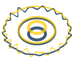
  $\varGamma$, as depicted in figure 1. We begin by extending the classical analysis of Crow (Reference Crow1970), where the rings are modelled as irrotational vortices in an incompressible, inviscid fluid. The velocity at any point along either ring is then given by the Biot–Savart law,
 \begin{equation} \boldsymbol{U_n}=\sum_{m=1}^2\frac{\varGamma_m}{4{\rm \pi}}\int \frac{\boldsymbol{D_{mn}}\times {\rm d}\boldsymbol{L_{m}}}{|\boldsymbol{D_{mn}}|^3}=\boldsymbol{e_x}u_n+ \boldsymbol{e_y}v_n+\boldsymbol{e_z}w_n, \end{equation}
where  $\boldsymbol {D_{mn}}$ is the displacement vector directed to a point on ring $m$ from a point on ring $n$;
$n$;  ${\rm d} \boldsymbol {L_n}$ is the differential tangent vector; $\boldsymbol {e_x}$, $\boldsymbol {e_y}$ and $\boldsymbol {e_z}$ are Cartesian unit vectors in the $x$,
$x$,  $y$,
$y$,  $z$ directions, respectively. Mathematically,
 \begin{align}
\left.\begin{array}{@{}c@{}}
\boldsymbol{d_n}=\boldsymbol{e_x}h_n(\theta_n,t)\cos{\theta_n}+
\boldsymbol{e_y}h_n(\theta_n,t)\sin{\theta_n}+\boldsymbol{e_z}s_n(\theta_n,t),\\
\boldsymbol{D_{mn}}=\boldsymbol{e_x}R(\cos{\theta_{m'}}-\cos{\theta_n})+
\boldsymbol{e_y}R(\sin{\theta_{m'}}-\sin{\theta_n})+
\boldsymbol{e_z}(z_m-z_n)+(\boldsymbol{d_{m'}}-\boldsymbol{d_n}),\\
{\rm d}\boldsymbol{L_{n}}=\left(-\boldsymbol{e_x}R\sin\theta_n+
\boldsymbol{e_y}R\cos{\theta_n}+\dfrac{\partial\boldsymbol{d_n}}{\partial
\theta_n}\right) {\rm d} \theta_n, \end{array}\right\}
\end{align}
\begin{align}
\left.\begin{array}{@{}c@{}}
\boldsymbol{d_n}=\boldsymbol{e_x}h_n(\theta_n,t)\cos{\theta_n}+
\boldsymbol{e_y}h_n(\theta_n,t)\sin{\theta_n}+\boldsymbol{e_z}s_n(\theta_n,t),\\
\boldsymbol{D_{mn}}=\boldsymbol{e_x}R(\cos{\theta_{m'}}-\cos{\theta_n})+
\boldsymbol{e_y}R(\sin{\theta_{m'}}-\sin{\theta_n})+
\boldsymbol{e_z}(z_m-z_n)+(\boldsymbol{d_{m'}}-\boldsymbol{d_n}),\\
{\rm d}\boldsymbol{L_{n}}=\left(-\boldsymbol{e_x}R\sin\theta_n+
\boldsymbol{e_y}R\cos{\theta_n}+\dfrac{\partial\boldsymbol{d_n}}{\partial
\theta_n}\right) {\rm d} \theta_n, \end{array}\right\}
\end{align}
where  $\theta _n=\tan ^{-1}({y_n}/{x_n})$; $h_n(\theta _n,t)$ is the perturbation amplitude in the $x$–
$x$– $y$ plane; $s_n(\theta _n,t)$ is the perturbation amplitude in the $z$ direction. The $m'$ subscript applies when $m=n$ (i.e. when evaluating the influence of one ring at a point on the same ring). Perturbations evolve under the constraint that they move at the local fluid velocity,
 \begin{equation} \frac{\partial \boldsymbol{d_n}}{\partial t}+u_n\frac{\partial \boldsymbol{d_n}}{\partial x_n}+v_n\frac{\partial \boldsymbol{d_n}}{\partial y_n}+w_n\frac{\partial \boldsymbol{d_n}}{\partial z_n}=\boldsymbol{e_x}u_n+\boldsymbol{e_y}v_n+\boldsymbol{e_z}w_n. \end{equation}
The set-up for the stability analysis showing two perturbed circular vortex cores with radius  $R$, core thickness $c$ and separation distance $b$ of equal and opposite circulation $\varGamma$.

Up to this point, the analysis accurately describes the system as long as the ratio between the core separation distance and the core thickness,  $b/c$, remains large. However, as the rings approach, this condition is violated. We therefore model the cross-section of each ring as a Lamb–Oseen vortex core with azimuthal vorticity
 \begin{equation} \omega(r,t)=\frac{\varGamma}{4{\rm \pi} \nu (t-t_0) (c/c_0)^2} \exp{\left[-\frac{r^2}{4 \nu (t-t_0) (c/c_0)^2}\right]}, \end{equation}
where  $r$ is the distance from the vortex core centre; $t$ is time; $t_0$ is the initial time; $\nu$ is the fluid viscosity; $c_0$ is the initial core thickness. The $c/c_0$ factor is a consequence of mass conservation and accounts for the concentration of vorticity due to changes in the vortex core thickness. The Lamb–Oseen core given in (2.4) is incorporated into the analysis by means of an effective core separation distance for the velocity in both the vertical and radial directions, $b_{ef,z}$ and $b_{ef,rad}$, respectively, similar to Widnall et al. (Reference Widnall, Bliss and Zalay1971). Physically, the effective core separation distance is the separation distance of an irrotational vortex core that induces the same velocity at the centre of the other core as given by a Lamb–Oseen vortex core at the separation distance. For example, the vertical velocity at the top core imparted by a bottom irrotational core separated by $b_{ef,z}$ is the same as that for a Lamb–Oseen vortex core separated by $b$. The effective separation distances are computed by equating the components of the following vector equation expressing the aforementioned velocity equivalence,
 \begin{equation} \frac{\varGamma_2}{4{\rm \pi}}\int\frac{\boldsymbol{D_{IR}}\times {\rm d}\boldsymbol{L_{IR}}}{|\boldsymbol{D_{IR}}|^3}=\frac{1}{4{\rm \pi}} \int_0^{R_{0.99\varGamma}}\int_0^{2{\rm \pi}}\int_0^{2{\rm \pi}}\omega(r,t)\frac{\boldsymbol{D_{LO}}\times {\rm d}\boldsymbol{L_{LO}}}{|\boldsymbol{D_{LO}}|^3}r \, {\rm d} \sigma \, {\rm d} r, \end{equation}
where
 \begin{equation} \left.\begin{array}{@{}c@{}} \boldsymbol{D_{IR}}=\boldsymbol{e_x}R(\cos{\theta_{2}}-\cos{\theta_1})+ \boldsymbol{e_y}R(\sin{\theta_{2}}-\sin{\theta_1})+ \boldsymbol{e_z}({-}b_{ef}),\\ {\rm d} \boldsymbol{L_{IR}}=(-\boldsymbol{e_x}R\sin\theta_2 +\boldsymbol{e_y}R\cos{\theta_2})\, {\rm d} \theta_2,\\ \begin{aligned} \boldsymbol{D_{LO}} & =\boldsymbol{e_x}[R(\cos{\theta_{2}}-\cos{\theta_1}) +r\cos \sigma\cos\theta_2]+\boldsymbol{e_y}[R(\sin{\theta_{2}}-\sin{\theta_1})\\ & \quad+r\cos\sigma\cos\theta_2] +\boldsymbol{e_z}({-}b+r\sin\sigma), \end{aligned}\\ {\rm d} \boldsymbol{L_{LO}}=[-\boldsymbol{e_x}(R+r\cos\sigma) \sin\theta_2+\boldsymbol{e_y}(R+r\cos\sigma)\cos{\theta_2}]\, {\rm d} \theta_2, \end{array}\right\} \end{equation} $\sigma$ is the angle within the core, $R_{0.99\varGamma }=\sqrt {-4\nu t (c/c_0)^2\ln (1-0.99)}$ is the radius that encloses 99 % of the Lamb–Oseen vortex circulation, which is sufficient for the convergence of the integral in (2.5), and $\theta _1$ can be any angle. We choose $\theta _1=0$, and $b_{ef}$ is understood to be $b_{ef,z}$ or $b_{ef,rad}$ for the vector component equations in the vertical, $\boldsymbol {e_z}$, or radial, $\boldsymbol {e_x}$, directions, respectively.
With the effective separation distances calculated, the analysis proceeds by equating (2.1) and (2.3) with substitutions from (2.2). The resulting equations are then linearized in the reference frame of the zero-order motion of the flow under the assumption that the zero-order motion is quasisteady compared with the first-order motion, which is verified later. A normal modes ansatz is assumed for the perturbations,  $\boldsymbol {d_n}=\boldsymbol {\tilde {d}_n}\, \textrm {e}^{at+\textrm {i}k\theta _n}$, where ${a=\alpha +\textrm {i}\mu}$, $\alpha$ is the growth rate, $\mu$ is the temporal frequency and $k$ is the integer wavenumber of the perturbation, resulting in an eigenvalue system of the form
 \begin{equation} a \begin{bmatrix}
\tilde{h}_1 \\ \tilde{s}_1 \\ \tilde{h}_2 \\ \tilde{s}_2
\end{bmatrix} = \begin{bmatrix} {\mathsf{M}}_{1,1} & {\mathsf{M}}_{1,2} & {\mathsf{M}}_{1,3}
& {\mathsf{M}}_{1,4} \\ {\mathsf{M}}_{2,1} & {\mathsf{M}}_{2,2} & {\mathsf{M}}_{2,3} & {\mathsf{M}}_{2,4} \\
{\mathsf{M}}_{3,1} & {\mathsf{M}}_{3,2} & {\mathsf{M}}_{3,3} & {\mathsf{M}}_{3,4} \\ {\mathsf{M}}_{4,1} & {\mathsf{M}}_{4,2}
& {\mathsf{M}}_{4,3} & {\mathsf{M}}_{4,4} \end{bmatrix} \begin{bmatrix}
\tilde{h}_1 \\ \tilde{s}_1 \\ \tilde{h}_2 \\ \tilde{s}_2
\end{bmatrix},
\end{equation}
\begin{equation} a \begin{bmatrix}
\tilde{h}_1 \\ \tilde{s}_1 \\ \tilde{h}_2 \\ \tilde{s}_2
\end{bmatrix} = \begin{bmatrix} {\mathsf{M}}_{1,1} & {\mathsf{M}}_{1,2} & {\mathsf{M}}_{1,3}
& {\mathsf{M}}_{1,4} \\ {\mathsf{M}}_{2,1} & {\mathsf{M}}_{2,2} & {\mathsf{M}}_{2,3} & {\mathsf{M}}_{2,4} \\
{\mathsf{M}}_{3,1} & {\mathsf{M}}_{3,2} & {\mathsf{M}}_{3,3} & {\mathsf{M}}_{3,4} \\ {\mathsf{M}}_{4,1} & {\mathsf{M}}_{4,2}
& {\mathsf{M}}_{4,3} & {\mathsf{M}}_{4,4} \end{bmatrix} \begin{bmatrix}
\tilde{h}_1 \\ \tilde{s}_1 \\ \tilde{h}_2 \\ \tilde{s}_2
\end{bmatrix},
\end{equation}
where the matrix coefficients are provided in the Appendix. General eigenvalues can be computed directly from (2.7), including for interactions that are asymmetric (e.g. rings with different radii, core thicknesses, strengths and lines of axisymmetry). However, due to the symmetry of the colliding rings in the present case,  ${\mathsf{M}}_{3,1}={\mathsf{M}}_{1,3}$, ${\mathsf{M}}_{3,2}=-{\mathsf{M}}_{1,4}$, ${\mathsf{M}}_{3,3}={\mathsf{M}}_{1,1}$, ${\mathsf{M}}_{3,4}=-{\mathsf{M}}_{1,2}$, ${\mathsf{M}}_{4,1}=-{\mathsf{M}}_{2,3}$, ${\mathsf{M}}_{4,2}={\mathsf{M}}_{2,4}$, ${\mathsf{M}}_{4,3}=-{\mathsf{M}}_{2,1}$ and ${\mathsf{M}}_{4,4}={\mathsf{M}}_{2,2}$. These coefficients may include integrals from (2.1), which are evaluated along the length of the vortex cores. For the planar case examined by Crow (Reference Crow1970), where the vortex cores are infinite lines extending in the $x$ direction, the integrals are evaluated from $x\in (-\infty,\infty )$. In the cylindrical case examined here, the integrals are evaluated from $\theta _n\in (0,2{\rm \pi} )$ when $m\neq n$. The cutoff model is used to represent the finite core thickness by evaluating the integral from $\theta _n\in (d/R,2{\rm \pi} -d/R)$ when $m=n$, circumventing the singularity in (2.1) when $|\boldsymbol {D_{mn}}|\rightarrow 0$ as in Crow (Reference Crow1970). In the classical analysis, the cutoff distance, $d$, is found by matching the translational velocity of a thin-core vortex ring to that predicted by the cutoff method (Kelvin Reference Kelvin1880; Crow Reference Crow1970). However, because the cores of rings that emerge from piston–cylinder devices relevant to experiments are not necessarily thin, we use a cutoff parameter that is a function of the core thickness calibrated to the translational velocity of the Norbury family of vortex rings (Norbury Reference Norbury1973), as shown in figure 2.
The cutoff parameter as a function of the core thickness.

As in the planar case (Crow Reference Crow1970), the eigenvalues associated with (2.4) can be combined into symmetric and antisymmetric modes,
 \begin{equation} \left.\begin{array}{@{}c@{}} \tilde{s}_{S}=\tilde{s}_{2}-\tilde{s}_{1},\tilde{h}_{S}=\tilde{h}_{2}+\tilde{h}_{1},\\ \tilde{s}_{A}=\tilde{s}_{2}+\tilde{s}_{1},\tilde{h}_{A}=\tilde{h}_{2}-\tilde{h}_{1}, \end{array}\right\} \end{equation}
respectively, yielding four roots,
 \begin{equation}
\left.\begin{array}{@{}c@{}} \begin{aligned} a_{S^\pm} & =
\tfrac{1}{2}\{{\mathsf{M}}_{1,1}+{\mathsf{M}}_{1,3}+{\mathsf{M}}_{2,2}-{\mathsf{M}}_{2,4}
\pm\{({\mathsf{M}}_{1,1}+{\mathsf{M}}_{1,3}+{\mathsf{M}}_{2,2}-{\mathsf{M}}_{2,4})^2\\
& \quad -4[({\mathsf{M}}_{1,1}+{\mathsf{M}}_{1,3})({\mathsf{M}}_{2,2}-{\mathsf{M}}_{2,4})-({\mathsf{M}}_{1,2}-{\mathsf{M}}_{1,4})({\mathsf{M}}_{2,1}
+{\mathsf{M}}_{2,3})]\}^{{1}/{2}}\}, \end{aligned}\\
\begin{aligned} a_{A^\pm} & = \tfrac{1}{2}\{{\mathsf{M}}_{1,1}-{\mathsf{M}}_{1,3}+{\mathsf{M}}_{2,2}+{\mathsf{M}}_{2,4}
\pm\{({\mathsf{M}}_{1,1}-{\mathsf{M}}_{1,3}+{\mathsf{M}}_{2,2}+{\mathsf{M}}_{2,4})^2\\
& \quad -4[({\mathsf{M}}_{1,1}-{\mathsf{M}}_{1,3})({\mathsf{M}}_{2,2}+{\mathsf{M}}_{2,4})-({\mathsf{M}}_{1,2}
+{\mathsf{M}}_{1,4})({\mathsf{M}}_{2,1}-{\mathsf{M}}_{2,3})]\}^{{1}/{2}}\}. \end{aligned}
\end{array}\right\}
\end{equation}
\begin{equation}
\left.\begin{array}{@{}c@{}} \begin{aligned} a_{S^\pm} & =
\tfrac{1}{2}\{{\mathsf{M}}_{1,1}+{\mathsf{M}}_{1,3}+{\mathsf{M}}_{2,2}-{\mathsf{M}}_{2,4}
\pm\{({\mathsf{M}}_{1,1}+{\mathsf{M}}_{1,3}+{\mathsf{M}}_{2,2}-{\mathsf{M}}_{2,4})^2\\
& \quad -4[({\mathsf{M}}_{1,1}+{\mathsf{M}}_{1,3})({\mathsf{M}}_{2,2}-{\mathsf{M}}_{2,4})-({\mathsf{M}}_{1,2}-{\mathsf{M}}_{1,4})({\mathsf{M}}_{2,1}
+{\mathsf{M}}_{2,3})]\}^{{1}/{2}}\}, \end{aligned}\\
\begin{aligned} a_{A^\pm} & = \tfrac{1}{2}\{{\mathsf{M}}_{1,1}-{\mathsf{M}}_{1,3}+{\mathsf{M}}_{2,2}+{\mathsf{M}}_{2,4}
\pm\{({\mathsf{M}}_{1,1}-{\mathsf{M}}_{1,3}+{\mathsf{M}}_{2,2}+{\mathsf{M}}_{2,4})^2\\
& \quad -4[({\mathsf{M}}_{1,1}-{\mathsf{M}}_{1,3})({\mathsf{M}}_{2,2}+{\mathsf{M}}_{2,4})-({\mathsf{M}}_{1,2}
+{\mathsf{M}}_{1,4})({\mathsf{M}}_{2,1}-{\mathsf{M}}_{2,3})]\}^{{1}/{2}}\}. \end{aligned}
\end{array}\right\}
\end{equation}
The coefficients  ${\mathsf{M}}_{1,1},{\mathsf{M}}_{1,3},{\mathsf{M}}_{2,2},{\mathsf{M}}_{2,4}\rightarrow 0$ with increasing ring radius, and the planar case is indeed recovered as $R\rightarrow \infty$.
In addition to the generalized roots in (2.9), a key difference distinguishing the cylindrical case from the classical planar case is the zero-order motion of the flow. In the planar case, the constant downward velocity of the vortex cores affects neither the core separation distance nor the core thickness and therefore does not alter the stability. In the present work, however, the motion of circular vortex cores causes their separation distance, radius and thickness to vary in time, resulting in time-dependent growth rates. The governing equations must therefore be integrated in time to determine the growth of perturbations along the vortex cores. The zero-order velocity can be determined using (2.1), substitutions from (2.2) with  $h_n,s_n=0$ (i.e. no perturbations) and the effective separation distance, and the cutoff method (Crow Reference Crow1970) with the Norbury-calibrated cutoff parameter. The integration is handled with a simple forward-Euler scheme that updates the ring radius and separation distance from the calculated radial and vertical velocities, respectively, at each time step. Since the flow is assumed incompressible, the core size is then updated to conserve the volume of the ring. The growth rates from (2.9) are then used to update the amplitudes of the perturbations of both the symmetric and antisymmetric modes, which are initialized as a uniform spectrum of amplitude $\sqrt {\tilde {s}_S^2+\tilde {h}_S^2}=\sqrt {\tilde {s}_A^2+\tilde {h}_A^2}=q_0$. The number of vortex rings emerging as a result of the CI is taken to correspond to the wavenumber of the mode that first reaches an amplitude of the order of the ring separation distance. Spurious high-frequency unstable modes (i.e. unstable modes occurring at larger wavenumbers than those of the high-frequency symmetric and antisymmetric modes) are ignored as in Crow (Reference Crow1970).
Before proceeding to the results of the analysis, a note on viscosity is warranted. As described, the influence of viscosity is incorporated via the effect of the relaxation of the core vorticity profile on the zero-order motion of the flow. Although viscous analysis is not applied directly to perturbations, this treatment maintains the applicability of the Biot–Savart law, which cannot strictly be applied to enforce the kinematic constraint on perturbations, (2.3), in a viscous flow (Sengupta Reference Sengupta2021). This limitation is demonstrated by a variety of flows including, for example, a vortex in the vicinity of a boundary layer (Lim, Sengupta & Chattopadhyay Reference Lim, Sengupta and Chattopadhyay2004; Sengupta, Bhumkar & Sengupta Reference Sengupta, Bhumkar and Sengupta2012). Even when the Reynolds number is high, the Biot–Savart law is insufficient to describe these vortex dynamics, and considering the viscous term in the vorticity transport equation is necessary for an accurate description of the flow profile and its receptivity to perturbation growth (Sengupta Reference Sengupta2021). However, nowhere in the present flow involving colliding vortex rings is there a region where the action of viscosity is as important as that near a no-slip boundary. The Biot–Savart law is therefore expected to accurately capture the perturbation growth via the CI that is the subject of the present study, which is validated by comparison with experiments (McKeown et al. Reference McKeown, Ostilla-Mónico, Pumir, Brenner and Rubinstein2018) in the results that follow.
3. Results
After verifying the zero-order motion of the flow, the growth of perturbations is examined for a collision involving two vortex rings of relatively low strength (i.e. circulation). Later, a collision of stronger vortex rings is examined in the context of a mechanism that may contribute to the transition of the flow to a turbulent puff.
3.1. Zero-order motion
We examine a set of initial conditions approximately matching the experiments of McKeown et al. (Reference McKeown, Ostilla-Mónico, Pumir, Brenner and Rubinstein2018) where the initial geometry is given by  $R_0=17.5$ mm, $c_0=7.0$ mm and $b_0=70.0$ mm. The rings in this experiment are generated from a piston–cylinder device submerged in a water tank with a stroke-to-diameter ratio $SR=2.5$, and the Reynolds number based on the diameter of the cylinder, the piston velocity and the viscosity of water is $Re=4000$. The model of Didden (Reference Didden1979, Reference Didden1982) can be used to estimate the ring circulation as
 \begin{equation} \varGamma=\left(1.14+\frac{0.32}{SR}\right)Re\, \nu, \end{equation}
where  $\nu =1.0\ \textrm {mm}^{2}\ \textrm {s}^{-1}$ and $t_0$ is chosen such that the vorticity profile within the cores matches experiments at $t=0$, see (2.4). Figure 3(a) shows the zero-order motion of the flow, i.e. the time evolution of the radius, separation distance and core thickness. Initially, when the separation distance is large, the vortex rings propagate at a nearly constant velocity with minimal change in their radii or core thicknesses, consistent with the motion of two isolated, steady vortex rings. As they approach, however, their translational speed decreases and their radii begin to increase due to the influence of each ring on the other, as shown in figure 3(b). After a period of rapidly increasing radial velocity, the ring radii increase at a nearly constant rate as their separation distance approaches a nearly constant value. After $t\approx 1.0$ s, the agreement between the model and the experimental data diverges slightly. This time, however, corresponding to a ring radius of approximately 80 mm, is consistent with the visible onset of the instability (McKeown et al. Reference McKeown, Ostilla-Mónico, Pumir, Brenner and Rubinstein2018), as evidenced by the sudden shift in the vertical location of the ring cores (figure 3c), and the increase in the scatter in the experimental core thickness data (figure 3d). Finally, figure 3(e) shows the values of $b_{ef,z}$ and $b_{ef,rad}$. Early in time, when the rings are far apart, the effective separation distance is near the value of the separation distance. Physically, this behaviour is a result of the velocity field from one ring at the location of the other for both an irrotational vortex and a Lamb–Oseen vortex being similar. As the rings approach, however, the velocity field from the Lamb–Oseen core diverges from that of an irrotational core because of the weighted influence of the vorticity in the core nearer to the other ring. This discrepancy causes the effective radial separation distance to decrease while the effective vertical separation distance increases. As the rings continue their approach, both effective separation distances decrease to a constant value. The agreement between the model and experiments in figure 3(b–d) demonstrates that the zero-order motion of the present system adequately represents physical experiments.
The zero-order motion for colliding rings (a), ring radius versus time for irrotational (solid line) and Lamb–Oseen (dashed line) vortices (b), vertical position of the upper (yellow solid line) and lower (blue dashed line) rings versus ring radius for Lamb–Oseen vortices (c), core thickness versus ring radius (d) and the vertical (dashed line) and radial (solid line) effective separation distances (e) for rings with  $R_0=17.5$ mm, $b_0=70.0$ mm, $c_0=7.0$ mm and $Re=4000$. Experimental data (orange dots) (McKeown et al. Reference McKeown, Ostilla-Mónico, Pumir, Brenner and Rubinstein2018) are provided for comparison (b–d). In (a), each subsequent image from left to right is 200 ms later in time than the previous.

Figure 3(b) also shows the ring radius as a function of time assuming  $b_{ef}=b$, i.e. the cores are assumed irrotational, as in the classical analysis. While this model works well for adequately separated cores, it breaks down as the rings approach, resulting in erroneously large ring radii. Because the vorticity within an irrotational vortex is confined to a line, there is no mechanism preventing the separation distance between the cores from approaching zero, at which point the rate at which the ring radii expand unphysically approaches infinity. The consideration of a finite-vorticity distribution within the cores is therefore essential to accurately describe the zero-order motion of this flow. Moreover, because the zero-order parameters of the flow affect the evolution of perturbations, see (2.9), their accurate description is required for the linear analysis, which is discussed next.
3.2. First-order motion
The evolution of linear perturbations (i.e. the first-order motion of the flow) is given as a function of wavenumber and time in figure 4. The analysis considers perturbation growth only from the CI and neglects instabilities associated with isolated vortex cores (Widnall Reference Widnall1975), including the curvature instability (Fukumoto & Hattori Reference Fukumoto and Hattori2005; Blanco-Rodríguez & Dizès Reference Blanco-Rodríguez and Dizès2017). Perturbations are initialized as a uniform spectrum with an amplitude of the order of the mean free path of the flow,  $q_0=0.13$ nm, which is also enforced as the minimum perturbation amplitude. Physical quantities are non-dimensionalized by the vortex ring circulation and initial radius. We examine the growth rates and perturbation amplitudes for both the symmetric and antisymmetric modes to illustrate the evolution of perturbations at three different non-dimensional times corresponding to the initial, intermediate and final stages of perturbation growth, $t_{Re=4000}^{init}$, $t_{Re=4000}^{inter}$, $t_{Re=4000}^{fin}$, respectively, as shown in figure 4(c, f).
The growth rates (a–c) and perturbation amplitudes (d–f) of the symmetric (a,d) and antisymmetric (b,e) modes for colliding rings with  $b_0/R_0=4$, $c_0/R_0=0.4$ and $Re=4000$. Lineouts in (c, f) correspond to $t_{Re=4000}^{init}=9.1$ (circles), $t_{Re=4000}^{inter}=13.3$ (squares) and $t_{Re=4000}^{fin}=16.7$ (triangles).

After the flow initially becomes unstable, three separate bands of spatial frequencies experience perturbation growth, as shown in figure 4 at time  $t_{Re=4000}^{init}=9.1$, indicated by the line marked by circles. The symmetric mode is excited within a band extending from $k=1$ to some $k>1$, which we refer to as the low-frequency symmetric band, and a separate band between two higher frequencies, which we refer to as the high-frequency symmetric band. The antisymmetric mode is excited within a single range of frequencies, namely the antisymmetric band, in the vicinity of the high-frequency symmetric band. At any given time, the wavenumber with the fastest growth rate exists within the antisymmetric band. The amplitudes of these excited modes increase, with the largest growth experienced by the wavenumber associated with the fastest growing mode within the antisymmetric band.
At time  $t_{Re=4000}^{inter}=13.3$, indicated by the lines marked by squares in figure 4, growth rates increase primarily because of the decreasing separation distance. Furthermore, as the cores expand, they can support the growth of increasingly large wavenumbers. The high- and low-frequency bands of the symmetric mode merge, though there are still two local growth rate maxima. The fastest growth rate is still experienced by a wavenumber within the antisymmetric band; however, at this time, the wavenumber with the greatest amplitude exists within the symmetric band. By this time, the zero-order motion of the flow, while slow compared with the growth of perturbations, causes the antisymmetric band to migrate to an entirely different range of wavenumbers than at time $t_{Re=4000}^{init}$. The low-frequency symmetric band, however, excites a wider range of wavenumbers that includes those excited at time $t_{Re=4000}^{init}$. As a result, although these wavenumbers are never growing as fast as the maximally excited wavenumber within the antisymmetric band, they grow for a longer period of time and therefore reach greater amplitudes.
The final time examined,  $t_{Re=4000}^{fin}=16.7$, indicated by the lines marked by triangles in figure 4, corresponds to the time when the perturbation amplitude reaches the separation distance. The growth rates decrease from time $t_{Re=4000}^{inter}$ because the separation distance increases slightly as a result of the viscous relaxation of the Lamb–Oseen vortex core and a tendency of the colliding rings to rebound. The high- and low-frequency bands of the symmetric mode separate, and the increasing radii of the expanding cores enable all three bands to support growth at larger wavenumbers. As before, the antisymmetric band migrates to a different range of frequencies, along with the high-frequency band of the symmetric mode, while the low-frequency band of the symmetric mode is still causing perturbation growth at the lower frequencies excited at earlier times. As a result, the slower-growing symmetric mode dominates the linear evolution once the perturbations are large enough to be examined experimentally. The wavenumber with an amplitude that first reaches the separation distance, which we herein refer to as the emergent wavenumber, is associated with the symmetric mode and equal to $k^{emerg}=18$, which is consistent with the number of secondary rings observed in the experiments of McKeown et al. (Reference McKeown, Ostilla-Mónico, Pumir, Brenner and Rubinstein2018). The dimensional time at which this happens, $t\approx 1$ s, is also consistent with the visible onset of the instability.
Figure 5(a) shows the perturbed vortex cores at time  $t_{Re=4000}^{fin}$, where perturbations associated with each wavenumber are added together with a random phase angle. While the cores here are shown intersecting one another, in reality, a complex vortex reconnection process occurs when the cores come in contact that results in the original cores breaking up into a series of smaller, or secondary, vortex structures (Kida & Takaoka Reference Kida and Takaoka1994; Hussain & Duraisamy Reference Hussain and Duraisamy2011; van Rees et al. Reference van Rees, Hussain and Koumoutsakos2012; Yao & Hussain Reference Yao and Hussain2022). The number of these smaller structures can be reasonably approximated by the emergent wavenumber. However, because other wavenumbers also experience significant growth, the number of secondary structures, and their sizes, may vary, as seen in experiments (Lim & Nickels Reference Lim and Nickels1992; McKeown et al. Reference McKeown, Ostilla-Mónico, Pumir, Brenner and Rubinstein2018).
The vortex cores at a time when the amplitude of the emergent wavenumber is of the order of the core separation distance (a), the wavenumbers experiencing maximal growth in the low- (blue) and high-frequency (teal) symmetric band and the antisymmetric (red) band and the largest amplitude symmetric (yellow) and antisymmetric (green) wavenumbers (b), and the growth angle of the emergent wavenumber versus time (c). The thin black vertical dashed lines indicate the time represented in (a) and the thin horizontal black dashed line in (c) indicates  $\beta =0.86$ rad.

The means by which perturbations grow from their initial amplitudes to those represented in figure 5(a) is a complex process during which the wavenumber that grows the fastest, the maximal wavenumber  $k^{max}$, and the wavenumber with the greatest amplitude, the dominant wavenumber $k^{dom}$, vary in time for both the symmetric and antisymmetric modes, as shown in figure 5(b). The discretized appearance of the data results from the restriction of all wavenumbers to integer values. Initially, the dominant wavenumber of the symmetric mode, $k^{dom}_S$, exists in the low-frequency symmetric band, lagging behind the maximal wavenumber within that band, $k^{max}_{S,lf}$, due to the expansion of the ring radius constantly pushing the maximal wavenumber to greater values. The dominant wavenumber of the symmetric mode abruptly shifts to greater wavenumbers after approximately $t\varGamma /R_0^2=10.1$, when growth from the high-frequency symmetric band becomes dominant. For a period of time, the dominant wavenumber of the symmetric mode experiences perturbation growth from a combination of the low- and high-frequency bands of the symmetric mode, which merge to excite an unbroken range of wavenumbers. The gap in the maximal wavenumber of the low-frequency symmetric band from ${t\varGamma /R_0^2=12.2}$ to $t\varGamma /R_0^2=12.5$ results from the single maximum in the combined symmetric band associated with the high-frequency symmetric band. Throughout the duration of the merged symmetric band, the influence of the high-frequency maximal wavenumber, $k^{max}_{S,hf}$, wanes while that of the low-frequency maximal wavenumber waxes, until the growth experienced by the dominant wavenumber of the symmetric mode is once again controlled by the low-frequency symmetric band after the symmetric bands split at $t\varGamma /R_0^2=15.8$. At this point, the growing ring radius tends to increase the maximal wavenumber of the low-frequency symmetric band, and a slight increase in separation distance, caused by the viscous relaxation of the vortex cores and the tendency of the cores to rebound slightly after reaching a minimum separation distance, tends to decrease the maximal wavenumber of the low-frequency symmetric band. These competing influences cause the maximal wavenumber of the low-frequency symmetric band to decrease slightly starting around $t\varGamma /R_0^2=13.3$ before increasing again after $t\varGamma /R_0^2=18.2$. At the time when the amplitude of the dominant mode reaches the separation distance, $t_{Re=4000}^{fin}$, the dominant wavenumber and the maximal wavenumber of the low-frequency symmetric band are nearly the same, a coincidence elaborated on in § A4.
The evolution of the antisymmetric mode is more straightforward. Caused primarily by the expansion of the ring, both the dominant and maximal wavenumbers of the antisymmetric band,  $k^{dom}_{A}$ and $k^{max}_{A}$, respectively, migrate to larger values as time progresses. However, at around $t\varGamma /R_0^2=14.6$, the growth rate of the maximal wavenumber is small enough compared with the rate at which the maximal wavenumber migrates to greater wavenumbers such that the dominant wavenumber ceases to increase beyond a value of $k^{dom}_{A}=40$.
As in the planar case, perturbed modes grow at an angle given by  $\beta =\tan ^{-1}({s}/{h})$, shown in figure 5(c) for the emergent wavenumber, $\beta _{S}^{18}$ (the subscript ‘S’ indicates the symmetric mode while the superscript ‘18’ is the emergent wavenumber). In the planar case, the low-frequency symmetric mode grows at an angle of $\beta =0.86$ rad. The emergent wavenumber similarly grows at $\beta =0.86$ rad when it is maximally excited, which occurs at $t\varGamma /R_0^2=9.0,12.7,15.5$ and $16.9$, but in general, the growth angle varies in time.
The analysis assumes that the zero-order motion is slow compared with the growth of perturbations, which we now verify. Figure 6(a) shows the radius, separation distance, core thickness and amplitude of the emergent wavenumber as a function of time. Between the time when perturbations first become unstable,  $t\varGamma /R_0^2=7.1$, and time $t_{Re=4000}^{fin}$, indicated by the thin, vertical black dashed line, the radius increases by a factor of 3.57, the separation distance decreases by a factor of 3.00, the core thickness decreases by a factor of 1.89, and the amplitude of the emergent wavenumber increases by a factor of $3.33\times 10^7$. On average, the relevant perturbations therefore evolve $10^6$ times faster, relative to their initial value, than the zero-order motion of the flow, verifying the assumption of quasisteadiness.
The radius (purple dot–dashed line), separation distance (yellow dashed line), core thickness (orange dotted line) and emergent perturbation amplitude (blue solid line) (a) and the product of the emergent perturbation amplitude and wavenumber (b) versus time. The thin vertical black dashed line indicates the time when the amplitude of the emergent wavenumber is of the order of the separation distance,  $t_{Re=4000}^{fin}$, and the thin horizontal black dashed line indicates an amplitude–wavenumber product of $0.1$.

We further verify that perturbations remain in the linear regime throughout the growth process. Figure 6(b) shows the amplitude–wavenumber product,  $q_{S}^{18}k^{18}$, of the emergent wavenumber as a function of time. We considered perturbations to be linear so long as this product remains less than 0.1 (i.e. linear terms are an order of magnitude larger than leading nonlinear terms), indicated by the horizontal dashed line. The amplitude–wavenumber product of the emergent wavenumber is equal to 0.1 at time $t\varGamma /R_0^2=16.5$. This indicates that the linear analysis begins to break down just prior to time $t_{Re=4000}^{fin}=16.7$. However, it is unlikely that the dominant wavenumber changes significantly between these two times. The linear assumption is therefore verified for nearly the entire duration of the flow leading up to the emergence of secondary vortex structures, the number of which is expected to be set by the emergent wavenumber.
3.3. Collisions of strong vortex rings
We now examine the collision of two vortex rings with the same initial geometry as the previous case but with a higher Reynolds number of  $Re=24\,000$, at which a turbulent puff, as opposed to an array of secondary vortex structures, is expected experimentally (Lim & Nickels Reference Lim and Nickels1992; McKeown et al. Reference McKeown, Ostilla-Mónico, Pumir, Brenner and Rubinstein2018, Reference McKeown, Ostilla-Mónico, Pumir, Brenner and Rubinstein2020). The initial core vorticity profile, see (2.4), is set by assuming that the vortex ring reaches the initial separation distance in an initial time that is inversely proportional to the vortex ring velocity (i.e. $t_0$ is inversely proportional to $Re$). As before, the evolution of the first-order motion is given as growth rates and perturbation amplitudes for both the symmetric and antisymmetric modes as functions of time and wavenumber in figure 7, and we similarly examine three distinct non-dimensional times, $t_{Re=24\,000}^{init}$, $t_{Re=24\,000}^{inter}$, $t_{Re=24\,000}^{fin}$, after the onset of perturbation growth. Similar to the lower-Reynolds-number case, three separate spatial frequency bands (low-frequency symmetric, high-frequency symmetric and antisymmetric) initially experience perturbation growth at time $t_{Re=24\,000}^{init}$, indicated by the line marked by circles in figure 7, when the fastest-growing and greatest-amplitude wavenumbers are those associated with the antisymmetric mode. Shortly after, the high- and low-frequency bands of the symmetric mode merge. Moreover, by time $t_{Re=24\,000}^{inter}$, indicated by the line marked by squares in figure 7, the symmetric mode has a single maximum. At this point, the wavenumber with the greatest amplitude is associated with the symmetric mode for the same reasons as described in the lower-Reynolds-number case.
The growth rates (a–c) and perturbation amplitudes (d–f) of the symmetric (a,d) and antisymmetric (b,e) modes for two colliding rings with  $b_0/R_0=4$, $c_0/R_0=0.4$ and $Re=24\,000$. Lineouts in(c, f) correspond to $t_{Re=24\,000}^{init}=8.6$ (circles), $t_{Re=24\,000}^{inter}=11.2$ (squares) and $t_{Re=24\,000}^{fin}=13.3$ (triangles).

Beyond time  $t_{Re=24\,000}^{inter}$, however, the nature of the solution changes compared with the lower-Reynolds-number case. While the increasing radius of the ring still tends to shift the antisymmetric band to higher wavenumbers, the decreased influence of the viscous relaxation of the vorticity within the Lamb–Oseen vortex cores yields relatively thinner cores, resulting in a tendency to excite lower wavenumbers. At the same time, because the cores are thinner, they can come into closer contact with one another, decreasing the separation distance, which causes greater growth rates overall and pushes the bands to higher wavenumbers. The overall effect of this competition results in the antisymmetric band still migrating towards higher wavenumbers, but exciting a wider range of wavenumbers and lingering on lower wavenumbers long enough to cause significantly more growth than the lower-Reynolds-number case. By the time the perturbation grows to be of the order of the separation distance at time $t_{Re=24\,000}^{fin}$, indicated by the line marked by triangles in figure 7, the amplitude of the antisymmetric mode exceeds that of the symmetric mode and the emergent wavenumber is therefore associated with the higher-frequency, faster-growing antisymmetric mode.
The variation of the emergent wavenumber with the Reynolds number, shown in figure 8, has implications relevant to experimental observations. Our analysis correctly predicts the increase in the emergent wavenumber with increasing Reynolds number observed in experiments (Lim & Nickels Reference Lim and Nickels1992; McKeown et al. Reference McKeown, Ostilla-Mónico, Pumir, Brenner and Rubinstein2018). Physically, the reason for this behaviour is that the tendency of the expanding ring to excite larger wavenumbers becomes relatively more important than the tendency of the viscous relaxation of the vorticity in the cores to excite lower wavenumbers as the Reynolds number increases. Because the emergent wavenumber at these Reynolds numbers is associated with the symmetric mode, vortex reconnection causes the separation of a number of secondary vortex structures roughly equal to the emergent wavenumber, though some variation will exist due to other wavenumbers also experiencing significant growth. Specifically, the variation in the number and size of secondary vortex structures will likely scale with the width of the perturbation amplitude spectrum.
The emergent wavenumber (blue solid line) and the amplitude of the symmetric (red dashed line) and antisymmetric (red dotted line) modes when  $q=b$. The black dashed line indicates $Re=8000$.

Our analysis also predicts a sharp transition to emergent wavenumbers associated with the antisymmetric mode that is consistent with the experimentally observed transition to a turbulent puff (Lim & Nickels Reference Lim and Nickels1992; McKeown et al. Reference McKeown, Ostilla-Mónico, Pumir, Brenner and Rubinstein2018). In the absence of the vortex reconnection that terminates the growth of the symmetric mode, the growth and stretching of this higher-wavenumber, faster-growing antisymmetric mode would rapidly continue into a nonlinear phase, possibly stimulating the turbulent puff. Furthermore, we note that while the maximum amplitude of perturbations experiencing antisymmetric growth,  $q_A^{dom}$, (red dotted line in figure 8) are up to five orders of magnitude smaller than their symmetric counterparts for the lower-Reynolds-number cases, the maximum amplitude of the perturbations experiencing symmetric growth, $q_S^{dom}$, (red dashed line in figure 8) is only up to one order of magnitude smaller than that of their dominating antisymmetric counterparts for the higher-Reynolds-number cases. As a result, near and beyond the Reynolds number where the flow becomes dominated by the antisymmetric mode, there is significant perturbation growth throughout a broader range of wavenumbers excited by both modes, further promoting the transition to a turbulent puff.
Experimentally, the transition to a turbulent puff is observed to occur near  $Re=8000$ (McKeown et al. Reference McKeown, Ostilla-Mónico, Pumir, Brenner and Rubinstein2018), indicated by the thin black dashed vertical line in figure 8, while our analysis predicts the transition to an antisymmetric dominated regime near $Re=22\,000$. This discrepancy may be attributed to a number of additional mechanisms that affect the flow leading up to a turbulent transition, which are discussed next.
The present analysis is restricted to circular vortex cores. However, core-shape deformations result from strain including that which is self-imposed and that imposed by the other ring, the effect of which increases as the cores approach, leading to deformation to elliptic or possibly even semicircular cores as seen in experiments (Chu et al. Reference Chu, Wang, Chang, Chang and Chang1995; McKeown et al. Reference McKeown, Ostilla-Mónico, Pumir, Brenner and Rubinstein2018). The failure of irrotational vortices to describe the zero-order motion in the present analysis, see figure 3(b), is evidence that the distribution of vorticity within the cores is critical, and extending this work to allow core-shape deformation would likely improve the characterization of the CI through a more accurate description of the zero-order motion.
Beyond the CI, core-shape deformations are manifested by additional instabilities. The curvature instability has been shown to affect vortex rings in excess of  $Re>6000$ (Blanco-Rodríguez & Dizès Reference Blanco-Rodríguez and Dizès2017). While the growth rate is smaller than that of the CI for the cases presently examined, the curvature instability could still excite perturbation growth that contributes to a turbulent transition near $Re=8000$. In addition, strain can cause the deformation of a single core into a multipolar structure (van Heijst, Kloosterziel & Williams Reference van Heijst, Kloosterziel and Williams1991; Orlandi & van Heijst Reference Orlandi and van Heijst1992; Carton & Legras Reference Carton and Legras1994; Sengupta et al. Reference Sengupta, Bhumkar and Sengupta2012). While such a structure is not visible in the vortex cores in the experiments of McKeown et al. (Reference McKeown, Ostilla-Mónico, Pumir, Brenner and Rubinstein2018, Reference McKeown, Ostilla-Mónico, Pumir, Brenner and Rubinstein2020), core deformations that could cause the formation of multiple poles may be present to an extent which, when coupled with other mechanisms, contributes to transition. The current analysis also neglects the strain-induced elliptic instability (Widnall et al. Reference Widnall, Bliss and Tsai1974), which is recognized, along with the CI, to primarily dominate vortex-pair interactions (Leweke et al. Reference Leweke, Le Dizes and Williamson2016), including the direct collision of vortex rings (Arun & Colonius Reference Arun and Colonius2023). A combined stability analysis that simultaneously considers these additional mechanisms, and possibly others, may be needed for a more complete description of the transition to a turbulent puff (Fukumoto & Hattori Reference Fukumoto and Hattori2005; Leweke et al. Reference Leweke, Le Dizes and Williamson2016; McKeown et al. Reference McKeown, Ostilla-Mónico, Pumir, Brenner and Rubinstein2018, Reference McKeown, Ostilla-Mónico, Pumir, Brenner and Rubinstein2020).
Lastly, the present analysis cannot accurately capture wavenumbers beyond a critical wavenumber–core-thickness product (Kelvin Reference Kelvin1880; Crow Reference Crow1970; Widnall et al. Reference Widnall, Bliss and Tsai1974), as discussed in § A4. Despite these limitations, the present analysis provides an accurate quantitative description of the lower-Reynolds-number case, correctly predicting the number of secondary vortex structures and the time scales on which they emerge, and may provide key insight into an additional mechanism, higher-frequency modes, affecting the transition of the flow to a turbulent puff, which are discussed in more detail next.
4. Higher-frequency modes and experimental implications
We further discuss the effect of the antisymmetric and the high-frequency symmetric modes on the evolution of the perturbation spectrum of the CI. The original analysis of Crow (Reference Crow1970) notes that the fastest-growing wavenumber is that associated with the antisymmetric mode, though the emergent wavenumber in aeroplane wakes is consistent with the low-frequency symmetric mode. At the time, this was attributed to the structure of atmospheric turbulence imposing an initial perturbation spectrum that favours low-frequency modes (Crow Reference Crow1970). Later, Widnall et al. (Reference Widnall, Bliss and Tsai1974) pointed out that the unstable high-frequency antisymmetric mode is spurious due to Crow's use of the low-frequency approximation of the dispersion relation describing the propagation of waves around a columnar vortex to calibrate the cutoff model for the self-induction integral (Kelvin Reference Kelvin1880; Crow Reference Crow1970). Figure 9 shows the rotation rate for a disturbance,  $\tau$, travelling around a constant-vorticity columnar vortex with rotation rate $\varOmega$ calculated from the exact dispersion relation and from the low-wavenumber approximation (Moore & Saffman Reference Moore and Saffman1972). The dominant antisymmetric mode in Crow's analysis for an elliptically loaded wing (Spreiter & Sacks Reference Spreiter and Sacks1951) is predicted to grow with a wavenumber–core-thickness product of $kc=3.34$, where in the planar case $k$ is the dimensional wavenumber (Crow Reference Crow1970). As figure 9(a) shows, the rotation rate of the disturbance predicted by the low-wavenumber approximation is zero when the product of the wavenumber and core thickness is 1.44. Beyond this value, the low-wavenumber approximation is in complete disagreement with the exact rotation rate, confirming the assertion that the high-frequency antisymmetric mode in Crow's analysis is indeed spurious (Widnall et al. Reference Widnall, Bliss and Tsai1974).
The exact rotation rate of a disturbance propagating about a constant-vorticity column (black solid line), the rotation rate from the long-wavelength limit (black dashed line) and the per cent difference between the two (black dotted line) versus the product of the wavenumber and core thickness (a) and the product of the wavenumber and core thickness (solid lines) and the per cent difference between the exact and long-wavelength-limit rotation rates (dashed lines) for a wavenumber of  $k=69$ (red lines) and $k=30$ (blue lines) versus time for the $Re=24\,000$ case (b). Arrows indicate corresponding axes.

In the present work, however, the product of the wavenumber and core thickness for the emergent wavenumber of the antisymmetric mode for the  $Re=24\,000$ case, $k^{emerg}=69$, never exceeds 0.8. As figure 9(b) shows, the error in the disturbance rotation rate from the low-wavenumber approximation decreases from $39\,\%$ to $5\,\%$ while the emergent wavenumber is experiencing perturbation growth. For comparison, the error for the dominant wavenumber of the symmetric mode, $k^{dom}_{S}=30$, decreases from $12\,\%$ to $1\,\%$, also shown in figure 9(b). The low wavelength–core-thickness product for the present cylindrical case, compared with the planar case, is largely caused by the tendency of the core thickness to decrease as the cores expand. The antisymmetric mode is therefore not necessarily spurious for colliding vortex rings and may play a role in the experimentally observed sharp transition to a turbulent puff as described earlier. It is possible that a stability analysis for colliding vortex rings utilizing the exact dispersion relation may indeed show that the antisymmetric mode never dominates the low-frequency symmetric mode, but as figure 9 indicates, the antisymmetric mode may still cause a potentially significant amount of growth in the perturbation spectrum that may contribute to the transition to a turbulent puff.
Furthermore, the effect of the zero-order motion of two colliding vortex rings on the stability provides additional insight for both the planar case and more general flows. While the vertical translation of two planar cores does not explicitly affect the stability, other factors may in the applications. For example, wingtip vortices may encounter background flows causing their separation distance to change, which would suppress the emergence of instability modes exciting narrow, higher-frequency wavenumber bands (if they are not already spurious). The viscous relaxation of a vortex core may have the same effect, as it does in the present work. An accurate characterization of the perturbation spectrum for any number of interacting vortex cores would generally require such considerations.
The first experiments demonstrating the CI along colliding vortex rings (Lim & Nickels Reference Lim and Nickels1992) utilized the radius, core separation distance and core thickness, once perturbations were visible, in a planar analysis (Crow Reference Crow1970) and found reasonable agreement between the fastest growing wavenumber of the low-frequency symmetric mode and the number of secondary vortex structures. This agreement, however, may be partially coincidental, i.e. the dominant and maximal wavenumbers for the low-frequency symmetric mode happen to be similar at the time when the perturbations are visible in experiments, as shown in figure 5. The present analysis provides a complete description of the time-dependent growth rate of the emergent wavenumber, and all other wavenumbers, from the beginning stages of perturbation growth, enabling a prediction of the fluid dynamics rather than postexperimental analysis only. Furthermore, integrating these growth rates in time fully characterizes the modal content of the perturbation spectrum, on top of which additional instabilities and nonlinearities develop and cause the flow to transition to a turbulent state. Future studies may therefore examine these nonlinear dynamics in the context of the present CI-modulated flow and utilize non-modal analysis to determine what similarities, if any, exist between transition in more thoroughly studied wall-bounded flows (Schmid Reference Schmid2007; Sengupta, Sundaram & Sengupta Reference Sengupta, Sundaram and Sengupta2020) and vortex core interactions.
Finally, while the present work concerns the direct collision of two vortex rings approaching from an initially large separation distance, the analysis for an expanding vortex dipole formed from a radially diverging annular starting jet is identical, with an appropriate definition of the vortex cores in the dipole. Given the difficulties associated with precisely aligning two vortex ring generators for a direct collision, the latter may be a convenient, and possibly more controllable, experimental set-up for examining the vortex core interactions that are the subject of many recent studies (Brenner et al. Reference Brenner, Hormoz and Pumir2016; McKeown et al. Reference McKeown, Ostilla-Mónico, Pumir, Brenner and Rubinstein2018, Reference McKeown, Ostilla-Mónico, Pumir, Brenner and Rubinstein2020; Mishra et al. Reference Mishra, Pumir and Ostilla-Mónico2021; Nguyen et al. Reference Nguyen, Phan, Duong and Le2021; Qi et al. Reference Qi, Tan, Corbitt, Urbanik, Salibindla and Ni2022). Moreover, the growth of the CI along an annular starting jet may be relevant to certain astrophysical systems. In particular, the CI may affect mass accumulation along circumstellar tori emitted from stars such as Sanduleak -69 202 (McCray & Fransson Reference McCray and Fransson2016), WeBo 1 (Bond, Pollacco & Webbink Reference Bond, Pollacco and Webbink2003), Wolf-Rayet 140 (Lau et al. Reference Lau2022) and many others.
5. Conclusion
The linear stability of two colliding coaxial vortex rings of equal strength is examined. The analysis considers the effects of curvature, the zero-order motion, the distribution of vorticity in the cores, and viscosity within a framework that enables direct calculation of the eigenvalues of the system. Unlike the planar case for line vortices, the zero-order motion of the flow causes the growth rates of the symmetric and antisymmetric modes to vary. The equations are therefore integrated in time to elucidate the evolution of the perturbation spectrum.
The analysis is validated by comparison with existing experimental data showing good agreement with both the zero- and first-order motion of the flow, enabling a prediction of the number of secondary vortex structures that emerge following the collision of two vortex rings at low-to-moderate Reynolds numbers, which is found to be approximately equal to the calculated emergent wavenumber. The analysis additionally captures the evolution of all other wavenumbers and shows how the zero-order motion causes narrow unstable wavenumber bands, not necessarily spurious, to migrate. As a result, these bands stimulate some growth but, for low Reynolds numbers, never enough to be visible in experiments.
Moreover, the analysis provides key insights into the variation of the emergent wavenumber with the Reynolds number. In particular, the analysis correctly predicts the increase in the emergent wavenumber, and therefore the number of secondary vortex structures that emerge in experiments, with increasing Reynolds number. This behaviour is a physical consequence of the rings expanding to larger radii, and therefore being able to support perturbation growth at larger wavenumbers, faster than the time scales on which their cores relax under the influence of viscosity. Furthermore, the decreased separation distances at higher Reynolds numbers also cause the wavenumber bands excited by both the high-frequency symmetric and antisymmetric modes to widen, enabling them to excite faster growth for a long enough period of time such that the perturbation amplitudes are of the order of or exceed those of the low-frequency symmetric mode. This enhanced modal content may contribute to the experimentally observed transition of the flow to a turbulent puff.
Declaration of interests
The authors report no conflict of interest.
Funding
This work is funded by the U.S. Department of Energy (DOE) as part of the Stewardship Science Graduate Fellowship Program under grant no. DE-NA0003960 and the U.S. Department of Energy NNSA Center of Excellence under cooperative agreement number DE-NA0003869. The work of H.L. is based upon work supported by the National Science Foundation MPS-Ascend Postdoctoral Research Fellowship under grant no. 2138109.
Appendix A
Linearizing (2.3) in the reference frame of the zero-order motion of the flow (i.e. subtracting out zero-order terms) yields
 \begin{equation} \frac{\partial \boldsymbol{d_n}}{\partial t}=\boldsymbol{e_x}\frac{\partial h_n}{\partial t}\cos{\theta_n}+\boldsymbol{e_y}\frac{\partial h_n}{\partial t}\sin{\theta_n}+\boldsymbol{e_z}\frac{\partial s_n}{\partial t}=\boldsymbol{e_x}u_n+\boldsymbol{e_y}v_n+\boldsymbol{e_z}w_n. \end{equation}
Equating the velocity components of (A1) with (2.1) after substitution of (2.2) and linearization, again in the reference frame of the zero-order motion, yields
 \begin{align} \frac{\partial h_n}{\partial t}\cos{\theta_n}&=\sum_{m=1}^2\frac{\varGamma_m}{4{\rm \pi}}\int \left\{\left\{R\sin{\theta_{m'}}\frac{\partial s_{m'}}{\partial\theta_{m'}} -R\sin{\theta_n}\frac{\partial s_{m'}}{\partial\theta_{m'}}-R(s_{m'}-s_n) \cos{\theta_{m'}}\right.\right.\nonumber\\ & \quad \left.\left.-(z_m-z_n)\frac{\partial h_{m'}}{\partial\theta_{m'}}\sin{\theta_{m'}} -(z_m-z_n)h_{m'}\cos{\theta_{m'}}\right\}\right/ \{[(R\cos{\theta_{m'}}\nonumber\\ &\quad -R\cos{\theta_n})^2+(R\sin{\theta_{m'}}-R\sin{\theta_n})^2+(z_m-z_n)^2]^{3/2}\}\nonumber\\ &\quad +\{3R(z_m-z_n)\cos{\theta_{m'}}[R h_{m'}\cos^2{\theta_{m'}} -R(h_n+h_{m'})\cos{\theta_{m'}}\cos{\theta_n}\nonumber\\ &\quad +R h_n\cos^2{\theta_n}+R h_{m'}\sin^2{\theta_{m'}} -R(h_n-h_{m'})\sin{\theta_{m'}}\sin{\theta_n}\nonumber\\ &\quad +Rh_n\sin^2{\theta_n}+(s_{m'}-s_n)(z_m-z_n)]\}/\{[(R\cos{\theta_{m'}}\nonumber\\ &\quad - R\cos{\theta_n})^2+(R\sin{\theta_{m'}}-R\sin{\theta_n})^2+(z_m-z_n)^2]^{5/2}\} \left.\vphantom{\frac{\partial s_{m'}}{\partial\theta_{m'}}}\right\} {\rm d} \theta_{m'}, \end{align}
 \begin{align} \frac{\partial
s_n}{\partial t}&=
\sum_{m=1}^2\frac{\varGamma_m}{4{\rm \pi}}\int
\left\{\left\{R\cos{\theta_{m'}}\frac{\partial
h_{m'}}{\partial \theta_{m'}}
\sin{\theta_{m'}}+2Rh_{m'}\cos^2{\theta_{m'}}-R\cos{\theta_n}
\frac{\partial
h_{m'}}{\partial\theta_{m'}}\sin{\theta_{m'}}\right.\right.\nonumber\\
& \quad
-Rh_{m'}\cos{\theta_n}\cos{\theta_{m'}}-Rh_n\cos{\theta_n}
\cos{\theta_{m'}}-R\sin{\theta_{m'}}\frac{\partial
h_{m'}}{\partial \theta_{m'}}\cos{\theta_{m'}}\nonumber\\
&\quad
+2Rh_{m'}\sin^2{\theta_{m'}}+R\sin{\theta_n}\frac{\partial
h_{m'}}{\partial
\theta_{m'}}\cos{\theta_{m'}}-Rh_{m'}\sin{\theta_n}\sin{\theta_{m'}}\nonumber\\
&\quad - \left.\left. \vphantom{\frac{\partial
h_{m'}}{\partial \theta_{m'}}}
Rh_n\sin{\theta_n}\sin{\theta_{m'}}\right\}\right/
\{[(R\cos{\theta_{m'}}
-R\cos{\theta_n})^2+(R\sin{\theta_{m'}}
-R\sin{\theta_n})^2\nonumber\\ &\quad
+(z_m-z_n)^2]^{3/2}\}-\{3R^2(1-\cos{\theta_n}\cos{\theta_{m'}}-\sin{\theta_n}
\sin{\theta_{m'}})[R h_{m'}\cos^2{\theta_{m'}}\nonumber\\ &
\quad -R(h_n+h_{m'})\cos{\theta_{m'}}\cos{\theta_n}+R
h_n\cos^2{\theta_n} +R h_{m'}\sin^2{\theta_{m'}}\nonumber\\
&\quad -R(h_n-h_{m'})\sin{\theta_{m'}}\sin{\theta_n}+Rh_n
\sin^2{\theta_n}\nonumber\\
&\quad +(s_{m'}-s_n)(z_m-z_n)]\}/
\{[(R\cos{\theta_{m'}}\nonumber\\
&\quad -R\cos{\theta_n})^2+(R\sin{\theta_{m'}}-R\sin{\theta_n})^2+(z_m-z_n)^2]^{5/2}\}
\left.\vphantom{\frac{\partial h_{m'}}{\partial
\theta_{m'}}} \right\}{\rm d} \theta_{m'},
\end{align}
\begin{align} \frac{\partial
s_n}{\partial t}&=
\sum_{m=1}^2\frac{\varGamma_m}{4{\rm \pi}}\int
\left\{\left\{R\cos{\theta_{m'}}\frac{\partial
h_{m'}}{\partial \theta_{m'}}
\sin{\theta_{m'}}+2Rh_{m'}\cos^2{\theta_{m'}}-R\cos{\theta_n}
\frac{\partial
h_{m'}}{\partial\theta_{m'}}\sin{\theta_{m'}}\right.\right.\nonumber\\
& \quad
-Rh_{m'}\cos{\theta_n}\cos{\theta_{m'}}-Rh_n\cos{\theta_n}
\cos{\theta_{m'}}-R\sin{\theta_{m'}}\frac{\partial
h_{m'}}{\partial \theta_{m'}}\cos{\theta_{m'}}\nonumber\\
&\quad
+2Rh_{m'}\sin^2{\theta_{m'}}+R\sin{\theta_n}\frac{\partial
h_{m'}}{\partial
\theta_{m'}}\cos{\theta_{m'}}-Rh_{m'}\sin{\theta_n}\sin{\theta_{m'}}\nonumber\\
&\quad - \left.\left. \vphantom{\frac{\partial
h_{m'}}{\partial \theta_{m'}}}
Rh_n\sin{\theta_n}\sin{\theta_{m'}}\right\}\right/
\{[(R\cos{\theta_{m'}}
-R\cos{\theta_n})^2+(R\sin{\theta_{m'}}
-R\sin{\theta_n})^2\nonumber\\ &\quad
+(z_m-z_n)^2]^{3/2}\}-\{3R^2(1-\cos{\theta_n}\cos{\theta_{m'}}-\sin{\theta_n}
\sin{\theta_{m'}})[R h_{m'}\cos^2{\theta_{m'}}\nonumber\\ &
\quad -R(h_n+h_{m'})\cos{\theta_{m'}}\cos{\theta_n}+R
h_n\cos^2{\theta_n} +R h_{m'}\sin^2{\theta_{m'}}\nonumber\\
&\quad -R(h_n-h_{m'})\sin{\theta_{m'}}\sin{\theta_n}+Rh_n
\sin^2{\theta_n}\nonumber\\
&\quad +(s_{m'}-s_n)(z_m-z_n)]\}/
\{[(R\cos{\theta_{m'}}\nonumber\\
&\quad -R\cos{\theta_n})^2+(R\sin{\theta_{m'}}-R\sin{\theta_n})^2+(z_m-z_n)^2]^{5/2}\}
\left.\vphantom{\frac{\partial h_{m'}}{\partial
\theta_{m'}}} \right\}{\rm d} \theta_{m'},
\end{align}
noting that due to the problem symmetry, the equation for the velocity in the  $y$ direction is redundant and therefore omitted. Applying normal modes of the form $\boldsymbol {d_n}=\boldsymbol {\tilde {d}_n}\, \textrm {e}^{at+ik\theta _n}$ yields
 \begin{align} a\tilde{h}_1 \cos{\theta_1}&= \frac{\varGamma_1}{4{\rm \pi}}\int_{\theta_1+{d}/{R}}^{\theta_1+2{\rm \pi}-{d}/{R}} \{\{R\sin{\theta_{1'}}[-\tilde{s}_{1'}k\sin(k\theta_{1'})]-R\sin{\theta_1}[-\tilde{s}_{1'} k\sin(k\theta_{1'})]\nonumber\\ &\quad -R[\tilde{s}_{1'}\cos(k\theta_{1'})-\tilde{s}_1\cos(k\theta_1)]\cos(\theta_{1'})\}/\{[(R \cos{\theta_{1'}}\nonumber\\ &\quad -R\cos{\theta_1})^2+(R\sin{\theta_{1'}}-R\sin{\theta_1})^2]^{3/2}\}\}\,{\rm d} \theta_{1'}\nonumber\\ &\quad +\frac{\varGamma_2}{4{\rm \pi}}\int_{0}^{2{\rm \pi}} \{\{R\sin{\theta_{2'}}[-\tilde{s}_{2'}k\sin(k\theta_{2'})] -R\sin{\theta_1}[-\tilde{s}_{2'}k\sin(k\theta_{2'})]\nonumber\\ &\quad -R[\tilde{s}_{2'}\cos(k\theta_{2'})-\tilde{s}_1\cos(k\theta_1)] \cos(\theta_{2'})+b[-\tilde{h}_{2'}k\sin(k\theta_{2'})]\sin{\theta_{2'}}\nonumber\\ &\quad +b\tilde{h}_{2'}\cos(k\theta_{2'})\cos{\theta_{2'}}\}/ \{[(R\cos{\theta_{1'}}-R\cos{\theta_1})^2+(R\sin{\theta_{1'}}\nonumber\\ &\quad -R\sin{\theta_1})^2+b^2]^{3/2}\}-\{3Rb\cos{\theta_{2'}}[R\tilde{h}_{2'} \cos(k\theta_{2'})\cos^2{\theta_{2'}}\nonumber\\ &\quad -R(\tilde{h}_1\cos(k\theta_1)+\tilde{h}_{2'}\cos(k\theta_{2'})) \cos(\theta_{2'})\cos(\theta_1)+R\tilde{h}_1\cos(k\theta_1)\cos^2(\theta_1)\nonumber\\ &\quad +R\tilde{h}_{2'}\cos(k\theta_{2'})\sin^2{\theta_{2'}} -R(\tilde{h}_1\cos(k\theta_1)-\tilde{h}_{2'}\cos(k\theta_{2'})) \sin(\theta_{2'})\sin(\theta_1)\nonumber\\ &\quad +R\tilde{h}_1\cos(k\theta_1)\sin^2{\theta_1}-b(\tilde{s}_{2'} \cos(k\theta_{2'})-\tilde{s}_1\cos(k\theta_1))]\}/\{[(R\cos{\theta_{1'}}\nonumber\\ &\quad -R\cos{\theta_1})^2+(R\sin{\theta_{1'}}-R\sin{\theta_1})^2+b^2]^{5/2}\}\} \,{\rm d} \theta_{2'}, \end{align}
 \begin{align} a\tilde{s}_1&=\frac{\varGamma_1}{4{\rm \pi}}\int_{\theta_1+{d}/{R}}^{\theta_1+2{\rm \pi}-{d}/{R}} \{\{{-}R\cos{\theta_{1'}}\tilde{h}_{1'}k\sin(k\theta_{1'})\sin{\theta_{1'}} +2R\tilde{h}_{1'}\cos(k\theta_{1'})\cos^2{\theta_{1'}} \nonumber\\ &\quad + R\cos{\theta_1}\tilde{h}_{1'}k\sin(k\theta_{1'})\sin{\theta_{1'}} -R\cos{\theta_1}\tilde{h}_{1'}\cos(k\theta_{1'})\cos{\theta_{1'}} \nonumber\\ &\quad -\tilde{h}_1\cos(k\theta_1)\cos{\theta_1}R\cos{\theta_{1'}} +R\sin{\theta_{1'}}\tilde{h}_{1'}k\sin(k\theta_{1'})\cos{\theta_{1'}} \nonumber\\ &\quad +2R\tilde{h}_{1'}\cos(k\theta_{1'})\sin^2{\theta_{1'}} -R\sin{\theta_1}\tilde{h}_{1'}k\sin(k\theta_{1'})\cos{\theta_{1'}} \nonumber\\ &\quad -R\sin{\theta_1}\tilde{h}_1\cos(k\theta_{1'})\sin{\theta_{1'}} -R\sin{\theta_1}\tilde{h}_{1'}\cos(k\theta_{1'})\sin{\theta_{1'}}\}/ \{[(R\cos{\theta_{1'}} \nonumber\\ &\quad -R\cos{\theta_1})^2+(R\sin{\theta_{1'}}-R\sin{\theta_1})^2+b^2]^{3/2}\} -\{3R^2(1-\cos{\theta_1}\cos{\theta_{1'}} \nonumber\\ &\quad -\sin{\theta_1}\sin{\theta_{1'}})[R\tilde{h}_{1'}\cos(k\theta_{1'})\cos^2{\theta_{1'}} -R(\tilde{h}_1\cos(k\theta_1) \nonumber\\ &\quad +\tilde{h}_{1'}\cos(k\theta_{1'}))\cos(\theta_{1'})\cos(\theta_1) +R\tilde{h}_1\cos(k\theta_1)\cos^2(\theta_1) \nonumber\\ &\quad +R\tilde{h}_{1'}\cos(k\theta_{1'})\sin^2{\theta_{1'}} -R(\tilde{h}_1\cos(k\theta_1)-\tilde{h}_{1'}\cos(k\theta_{1'}))\sin(\theta_{1'})\sin(\theta_1) \nonumber\\ & \quad +R\tilde{h}_1\cos(k\theta_1)\sin^2{\theta_1}]\}/ \{[(R\cos{\theta_{1'}}-R\cos{\theta_1})^2+(R\sin{\theta_{1'}} \nonumber\\ &\quad -R\sin{\theta_1})^2+b^2]^{5/2}\}\}\,{\rm d} \theta_{1'} +\frac{\varGamma_2}{4{\rm \pi}}\int_{0}^{2{\rm \pi}} \{\{{-}R\cos{\theta_{2'}}\tilde{h}_{2'}k\sin(k\theta_{2'})\sin{\theta_{2'}} \nonumber\\ &\quad +2R\tilde{h}_{2'}\cos(k\theta_{2'})\cos^2{\theta_{2'}} + R\cos{\theta_1}\tilde{h}_{2'}k\sin(k\theta_{2'})\sin{\theta_{2'}} \nonumber\\ &\quad -R\cos{\theta_1}\tilde{h}_{2'}\cos(k\theta_{2'})\cos{\theta_{2'}} -\tilde{h}_1\cos(k\theta_1)\cos{\theta_1}R\cos{\theta_{2'}} \nonumber\\ &\quad +R\sin{\theta_{2'}}\tilde{h}_{2'}k\sin(k\theta_{2'})\cos{\theta_{2'}} +2R\tilde{h}_{2'}\cos(k\theta_{2'})\sin^2{\theta_{2'}} \nonumber\\ &\quad -R\sin{\theta_1}\tilde{h}_{2'}k\sin(k\theta_{2'})\cos{\theta_{2'}} -R\sin{\theta_1}\tilde{h}_1\cos(k\theta_{2'})\sin{\theta_{2'}} \nonumber\\ &\quad -R\sin{\theta_1}\tilde{h}_{2'}\cos(k\theta_{2'})\sin{\theta_{2'}}\}/ \{[(R\cos{\theta_{2'}} \nonumber\\ &\quad -R\cos{\theta_1})^2+(R\sin{\theta_{2'}}-R\sin{\theta_1})^2+b^2]^{3/2}\} -\{3R^2(1-\cos{\theta_1}\cos{\theta_{2'}} \nonumber\\ &\quad -\sin{\theta_1}\sin{\theta_{2'}})[R\tilde{h}_{2'}\cos(k\theta_{2'})\cos^2{\theta_{2'}} -R(\tilde{h}_1\cos(k\theta_1) \nonumber\\ &\quad +\tilde{h}_{2'}\cos(k\theta_{2'}))\cos(\theta_{2'})\cos(\theta_1) +R\tilde{h}_1\cos(k\theta_1)\cos^2(\theta_1)\nonumber\\ &\quad +R\tilde{h}_{2'}\cos(k\theta_{2'})\sin^2{\theta_{2'}}-R(\tilde{h}_1 \cos(k\theta_1)-\tilde{h}_{2'}\cos(k\theta_{2'}))\sin(\theta_{2'})\sin(\theta_1)\nonumber\\ &\quad +R\tilde{h}_1\cos(k\theta_1)\sin^2{\theta_1}-b(\tilde{s}_{2'}\cos(k\theta_{2'}) -\tilde{s}_1\cos(k\theta_1))]\}/ \{[(R\cos{\theta_{2'}} \nonumber\\ &\quad -R\cos{\theta_1})^2+(R\sin{\theta_{2'}}-R\sin{\theta_1})^2+b^2]^{5/2}\}\} \,{\rm d} \theta_{2'}. \end{align}
Complementary equations for  $\tilde {h}_2$ and $\tilde {s}_2$ are obtained from (A4) and (A5), respectively, by interchanging the subscripts 1 and 2 and by substituting $-b$ for $b$. The matrix entries for the eigenvalue problem (2.7) are then formed by collecting terms in (A4)-(A5) in the perturbation quantities and choosing $\theta _1=0$, giving
 \begin{align} {\mathsf{M}}_{1,1}&=\frac{\varGamma_2}{4{\rm \pi}}\int_0^{2{\rm \pi}}{\rm d}\theta_{2'} \{\{3R\cos{\theta_{2'}}-3R-3R\cos(k\theta_1)\sin^2{\theta_1}\} \nonumber\\ &\quad bR\cos{\theta_2'}/ \{[R\cos(\theta_{2'})-R]^2+[R\sin(\theta_{2'})]^2+b^2\}^{{5}/{2}}\}, \end{align}
 \begin{align} {\mathsf{M}}_{1,2}&=\frac{\varGamma_1}{4{\rm \pi}}\int_{{d}/{R}}^{2{\rm \pi}-{d}/{R}} {\rm d} \theta_{1'} \{\{{-}R\sin(\theta_{1'})k\sin(k\theta_{1'})-R\cos(k\theta_{1'})\cos(\theta_{1'})\nonumber\\ &\quad+R\cos(\theta_{1'})\}/ \{[R\cos(\theta_{1'})-R]^2+[R\sin(\theta_{1'})]^2\}^{{3}/{2}}\}\nonumber\\ &\quad + \frac{\varGamma_2}{4{\rm \pi}}\int_{0}^{2{\rm \pi}} {\rm d} \theta_{2'} \{\{R\cos(\theta_{2'})\}/\{[R\cos(\theta_{2'})-R]^2 +[R\sin(\theta_{2'})]^2\nonumber\\ &\quad+b^2\}^{{3}/{2}}\} + \frac{\varGamma_2}{4{\rm \pi}}\int_{0}^{2{\rm \pi}}{\rm d} \theta_{2'} \{{-}3R[b\cos(\theta_{2'})]^2/ \{[R\cos(\theta_{2'})-R]^2\nonumber\\ &\quad+[R\sin(\theta_{2'})]^2 +b^2\}^{{5}/{2}}\}, \end{align}
 \begin{align} {\mathsf{M}}_{1,3}&=\frac{\varGamma_2}{4{\rm \pi}}\int_{0}^{2{\rm \pi}}{\rm d}\theta_{2'} \{\{{-}bk\sin(k\theta_{2'})\sin(\theta_{2'})+b\cos(k\theta_{2'})\cos{\theta_{2'}}\}/ \{[R\cos(\theta_{2'})-R]^2\nonumber\\ &\quad+[R\sin(\theta_{2'})]^2+b^2\}^{{3}/{2}}\} + \frac{\varGamma_2}{4{\rm \pi}}\int_{0}^{2{\rm \pi}}{\rm d}\theta_{2'} \{bR\cos(\theta_{2'})\{{-}3R\cos(k\theta_{2'})\cos^2(\theta_{2'})\nonumber\\ &\quad+3R\cos(k\theta_{2'})\cos(\theta_{2'}) -3R\cos(k\theta_{2'})\sin^2(\theta_{2'})\}/ \{[R\cos(\theta_{2'})-R]^2\nonumber\\ &\quad+[R\sin(\theta_{2'})]^2+b^2\}^{{5}/{2}}\}, \end{align}
 \begin{align}
{\mathsf{M}}_{1,4}&=\frac{\varGamma_2}{4{\rm \pi}}\int_{0}^{2{\rm \pi}}{\rm d}
\theta_{2'} \{\{{-}R\sin(\theta_{2'})k\sin(k\theta_{2'})-R\cos(k\theta_{2'})\cos(\theta_{2'})\}/
\{[R\cos(\theta_{2'})-R]^2\nonumber\\
&\quad+[R\sin(\theta_{2'})]^2+b^2\}^{{3}/{2}}\} +
\frac{\varGamma_2}{4{\rm \pi}}\int_{0}^{2{\rm \pi}}{\rm d}\theta_{2'}
\{\{3b\cos(k\theta_{2'})\} bR\cos(\theta_{2'})/
\{[R\cos(\theta_{2'})\nonumber\\
&\quad -R]^2+[R\sin(\theta_{2'})]^2+b^2\}^{{5}/{2}}\},
\end{align}
\begin{align}
{\mathsf{M}}_{1,4}&=\frac{\varGamma_2}{4{\rm \pi}}\int_{0}^{2{\rm \pi}}{\rm d}
\theta_{2'} \{\{{-}R\sin(\theta_{2'})k\sin(k\theta_{2'})-R\cos(k\theta_{2'})\cos(\theta_{2'})\}/
\{[R\cos(\theta_{2'})-R]^2\nonumber\\
&\quad+[R\sin(\theta_{2'})]^2+b^2\}^{{3}/{2}}\} +
\frac{\varGamma_2}{4{\rm \pi}}\int_{0}^{2{\rm \pi}}{\rm d}\theta_{2'}
\{\{3b\cos(k\theta_{2'})\} bR\cos(\theta_{2'})/
\{[R\cos(\theta_{2'})\nonumber\\
&\quad -R]^2+[R\sin(\theta_{2'})]^2+b^2\}^{{5}/{2}}\},
\end{align} \begin{align} {\mathsf{M}}_{2,1}&=\frac{\varGamma_1}{4{\rm \pi}}\int_{{d}/{R}}^{2{\rm \pi}-{d}/{R}}{\rm d} \theta_{1'} \{\{{-}Rk\sin(k\theta_{1'})\sin(\theta_{1'})+R\cos(k\theta_{1'})\cos^2(\theta_{1'})\nonumber\\ &\quad +R\cos(k\theta_{1'})\cos^2(\theta_{1'})+Rk\sin(k\theta_{1'})\sin(\theta_{1'}) -R\cos(k\theta_{1'})\cos(\theta_{1'})\nonumber\\ &\quad -R\cos(\theta_{1'})+R\sin(\theta_{1'})k\sin(k\theta_{1'})\cos(\theta_{1'}) +R\cos(k\theta_{1'})\sin^2(\theta_{1'})\nonumber\\ &\quad +R\cos(k\theta_{1'})\sin^2(\theta_{1'})\}/ \{[R\cos(\theta_{1'})-R]^2 +[R\sin(\theta_{1'})]^2\}^{{3}/{2}}\}\nonumber\\ &\quad + \frac{\varGamma_1}{4{\rm \pi}}\int_{{d}/{R}}^{2{\rm \pi}-{d}/{R}}{\rm d} \theta_{1'} \{\{{-}3R\cos(k\theta_{1'})\cos^2(\theta_{1'})+3R\cos(\theta_{1'})\nonumber\\ &\quad +3R\cos(k\theta_{1'})\cos(\theta_{1'})-3R-3R\cos(k\theta_{1'}) \sin^2(\theta_{1'})\} \nonumber\\ &\quad\times R^2[1-\cos(\theta_{1'})]/\{[R\cos(\theta_{1'})-R]^2+[R\sin(\theta_{1'})]^2\}^{{5}/{2}}\}\nonumber\\ &\quad + \frac{\varGamma_2}{4{\rm \pi}}\int_{0}^{2{\rm \pi}}{\rm d} \theta_{2'} \{\{{-}R\cos(\theta_{2'})\}/ \{[R\cos(\theta_{2'})-R]^2+[R\sin(\theta_{2'})]^2 +b^2\}^{{3}/{2}}\}\nonumber\\ &\quad+ \frac{\varGamma_2}{4{\rm \pi}}\int_{0}^{2{\rm \pi}}{\rm d} \theta_{2'} \{\{3R\cos(\theta_{2'})-3R\}\times R^2[1-\cos(\theta_{1'})]/ \{[R\cos(\theta_{2'})-R]^2\nonumber\\ &\quad+[R\sin(\theta_{2'})]^2+b^2\}^{{5}/{2}}\}, \end{align}
 \begin{align} {\mathsf{M}}_{2,2}&=\frac{\varGamma_2}{4{\rm \pi}}\int_{0}^{2{\rm \pi}}{\rm d}\theta_{2'} \{{-}3bR^2[1-\cos(\theta_{1'})]/ \{[R\cos(\theta_{2'})-R]^2+ [R\sin(\theta_{2'})]^2+b^2\}^{{5}/{2}}\}, \end{align}
 \begin{align} {\mathsf{M}}_{2,3}&=\frac{\varGamma_2}{4{\rm \pi}}\int_{0}^{2{\rm \pi}}{\rm d}\theta_{2'} \{\{{-}R\cos(\theta_{2'})k\sin(k\theta_{2'})\sin(\theta_{2'}) +R\cos(k\theta_{2'})\cos^2(\theta_{2'})\nonumber\\ &\quad +R\cos(k\theta_{2'})\cos^2(\theta_{2'})+Rk\sin(k\theta_{2'})-R\cos(k\theta_{2'})\cos(\theta_{2'})\nonumber\\ &\quad+R\sin(\theta_{2'})k\sin(k\theta_{2'})\cos(\theta_{2'})+R\cos(k\theta_{2'})\sin^2(\theta_{2'})\nonumber\\ &\quad+R\cos(k\theta_{2'})\sin^2(\theta_{2'})\}/ \{[R\cos(\theta_{2'})-R]^2 +[R\sin(\theta_{2'})]^2+b^2\}^{{3}/{2}}\}\nonumber\\ &\quad+ \frac{\varGamma_2}{4{\rm \pi}}\int_{0}^{2{\rm \pi}}{\rm d}\theta_{2'} \{\{{-}3R\cos(k\theta_{2'})\cos^2(\theta_{2'})+3R\cos(k\theta_{2'})\cos(\theta_{2'})\nonumber\\ &\quad-3R\cos(k\theta_{2'})\sin^2(\theta_{2'})\}\times R^2 [1-\cos(\theta_{1'})]/\{[R\cos(\theta_{2'})-R]^2\nonumber\\ &\quad+[R\sin(\theta_{2'})]^2+b^2\}^{{5}/{2}}\}, \end{align}
 \begin{align} {\mathsf{M}}_{2,4}&=\frac{\varGamma_2}{4{\rm \pi}}\int_{0}^{2{\rm \pi}}{\rm d} \theta_{2'} \{\{3b\cos(k\theta_{2'})\} R^2[1-\cos(\theta_{1'})]/\{[R\cos(\theta_{2'})-R]^2\nonumber\\ &\quad +[R\sin(\theta_{2'})]^2+b^2\}^{{5}/{2}}\}. \end{align}


 Open access