


Introduction
Ice streams account for only 10% of the Antarctic ice sheet, but are areas of significantly enhanced flow that are responsible for nearly 90% of the ice-sheet drainage (Reference Morgan, Jacka, Akerman and ClarkeMorgan and others, 1982). Tracking the internal movement and deformation of ice streams is key to understanding how they operate and respond to external factors. The deformation history of ice is preserved as elastic anisotropy due to the crystal-preferred orientation (CPO) of ice crystals (e.g. Reference AlleyAlley, 1988). Therefore in situ detection of such anisotropy is desirable, as it offers insights into stress patterns and the behaviour of ice sheets over time and over large areas. It also provides a means of testing the influence of crystal fabric on patterns of ice-sheet flow (Reference Martin, Gudmundsson, Pritchard and GagliardiniMartin and others, 2009), information that is needed to calibrate ice-sheet modelling. Deformation along the margins of ice streams leads to crevassing and fracturing, and basal reflectors of radar and seismic signals have been attributed oriented crystal (CPO) fabrics (e.g. Reference KingKing, 2009; Reference Horgan, Anandakrishnan, Alley, Burkett and PetersHorgan and others, 2011). Here we investigate ice anisotropy in Rutford Ice Stream, West Antarctica, using observations of shear-wave anisotropy in recordings of icequakes.
Rutford Ice Stream is a major ice stream in West Antarctica that drains into the Ronne Ice Shelf. Situated in a deep trough between the Ellsworth Mountains and the Fletcher Promontory, this approximately 300 km long, 25 km wide and 2.5 km thick ice stream moves at speeds of up to 400m a–1. During the austral summer of 2008/09, a team from the British Antarctic Survey (BAS) deployed an array of three-component seismometers on Rutford Ice Stream (Reference Pritchard, Brisbourne, King, Gudmundsson and SmithPritchard and others, 2011; Reference BrisbourneBrisbourne, 2012). Many thousands of microseismic events (icequakes) were recorded during the experiment, which only lasted a few weeks. The slippage of ice over the underlying rock bed leads to icequakes, especially in spots where there is little fluid-saturated basal sediment to lubricate the sliding (Reference Anandakrishnan and BentleyAnandakrishnan and Bentley, 1993; Reference Anandakrishnan and AlleyAnandakrishnan and Alley, 1994; Reference Walter, Deichmann and FunkWalter and others, 2008). An attractive feature of icequakes is that they generate P- and S-waves, and many conventional tools from earthquake seismology can be applied to such data. We analyse shear-wave anisotropy using a high-quality subset of this dataset.
Elastic anisotropy is found in most parts of the solid Earth and can be caused by a range of mechanisms (Reference BackusBackus, 1962; Reference Blackman, Wenk and KendallBlackman and others, 2002; Reference Holtzman and KendallHoltzman and Kendall, 2010). We consider candidate crystal fabrics due to CPO found in ice as plausible mechanisms for anisotropy in an ice-stream environment. We also consider a more extrinsic mechanism where anisotropy can be caused by preferentially aligned cracks or melt films; the possibility of such oriented weaknesses will have ramifications for the disintegration of ice shelves fed by ice streams.
Mechanisms for Anisotropy in Ice
Anisotropy refers to a directional variation in wave speeds and leads to a more complicated description of wave propagation than that for isotropic media. Only two elastic parameters are required to describe wave propagation in an isotropic medium, whereas up to 21 independent elastic constants are required to describe wave propagation in anisotropic media. Perhaps the most telltale sign of anisotropy is the presence of two independently propagating shear waves (so-called shear-wave splitting). An initially polarized shear wave travelling through an isotropic medium will split into two orthogonally polarized shear waves as it impinges on a region of anisotropy. The polarization of the shear waves is diagnostic of the anisotropic symmetry and the delay time between the fast and slow shear waves is a proxy for the magnitude of the anisotropy and the extent of the anisotropic region.
It is well known that ice crystals are anisotropic and that they can exhibit a CPO fabric (e.g. Reference AlleyAlley 1988; Reference Budd and JackaBudd and Jacka, 1989; Reference Wilson and ZhangWilson and Zhang, 1994). Hexagonal ice (Ih), the form found naturally on Earth, has two principal crystal axes: a vertical c-axis and three a-axes separated by 1208 and normal to the c-axis. The c-axis provides a major axis of symmetry in the elastic properties of the crystal, and velocities are rotationally invariant around this axis (often termed transverse isotropy). The direction of fastest P-wave velocity is along the c-axis (3.89kms-1), and the slowest velocities are found in a ∼50° cone from the c-axis (3.74 kms-1). The direction of minimum (0kms-1) shear-wave splitting is along the c-axis, and the direction of maximum (0.24kms-1) shear-wave splitting (i.e. separation between the fast and slow shear wave) is ∼50° from the c-axis (Fig. 1a) The slowest shear-wave velocity is along the c-axis (1.81 kms-1), while the fastest (2.10kms-1) is midway between the c- and a-axes.

Fig. 1. Upper-hemisphere projections of the predicted shear-wave splitting due to the alignment of Ih crystal ice (produced using the MSAT package of Reference Walker and WookeyWalker and Wookey, 2012). Tick marks show the polarization of the fast shear wave. Red colours show regions of minimum shear-wave splitting, blue colours show regions of maximum splitting. The maximum and minimum values are also displayed below each projection. (a) Single crystal of Ih hexagonal ice. (b) The ‘cluster’ or ‘solid-cone’ model, which is due to the alignment of c-axes in a cone around the vertical direction. (c) The ‘girdle’ model where the a-axes are aligned in the horizontal direction parallel to the flow direction and the c-axes are aligned in a vertical plane perpendicular to this.
Ice crystals shear two orders of magnitude more easily along the basal plane (orthogonal to the c-axis) than on the other slip systems (Reference Duval, Ashby and AndermanDuval and others, 1983), which readily leads to a CPO primarily by dislocation glide (e.g. Reference Castelnau, Duval, Lebensohn and CanovaCastelnau and others, 1996). As ice sheets flow and deform, the constituent crystals will align depending on factors such as strain rates, temperature and the presence of fluids. The resulting CPO can be very effective in producing an anisotropic medium.
In the near-surface, ice has a random fabric of crystals where the c- and a-axes are distributed through all possible orientations. When stress is applied, 90% of the deformation is accommodated by slip on the basal plane parallel to an a-axis direction, restricted by neighbouring grains (Reference Wilson and MarmoWilson and Marmo, 2000). Flattening under gravity or weight causes ice crystals to rotate such that the c-axes rotate towards the compressive stress (i.e. vertical) and the a-axes rotate uniformly away from the compression into the perpendicular plane (Reference AlleyAlley, 1988). With depth and increasing hydrostatic pressure, the c-axes orient themselves into a cone about the vertical axis, forming a cluster fabric (Reference Wilson and MarmoWilson and Marmo, 2000) and producing a transversely isotropic medium with a vertical symmetry axis (a so-called vertical transversely isotropic (VTI) symmetry; Fig. 1b). The angle this cone makes to the vertical decreases with increasing hydrostatic pressure. In structural geology, such a CPO is known as a cluster fabric, whereas in glaciology this CPO is normally referred to as the solid-cone fabric (e.g. Reference Horgan, Anandakrishnan, Alley, Burkett and PetersHorgan and others, 2011). Compared with the single crystal anisotropy, the P- and S-wave anisotropy is less, but the overall symmetry of the anisotropy is similar. At even greater depths the effects of dynamic recrystallization may lead to a more random orientation in the c-axes and hence a weaker overall anisotropy (Reference Anandakrishnan, Fitzpatrick, Alley, Gow and MeeseAnandakrishnan and others, 1994).
In an ice stream, the ice can also be confined perpendicular to the flow (stress) direction, resulting in simple shear (Reference AzumaAzuma, 1994). As such, the a-axes develop a preferred orientation parallel to the flow and the c-axes rotate into a girdle distribution orthogonal to the flow direction (Reference AlleyAlley, 1988; Reference Wilson and MarmoWilson and Marmo, 2000) (Fig. 1c). This effectively produces a transversely isotropic medium with a horizontal symmetry axis, which is often referred to as horizontal transversely isotropic (HTI) symmetry. In this model the fastest P-wave (3.88kms–1) is orientated in the ice-flow or a-axis direction. The vertical plane parallel to the flow direction is the plane of maximum shear-wave splitting (0.08kms–1).
Reference AzumaAzuma (1994) derived a flow law for anisotropic ice and developed a model of ice fabric distributions within a flowing ice stream (Fig. 2) based on the flow law predictions for three different flow regimes: (1) divergent flow from the theoretical point source of an ice stream/glacier; (2) parallel flow in the laterally constricted area of an ice stream/glacier; and (3) convergent flow to the theoretical point outlet of an ice stream/glacier. As can be seen in Figure 2 the lower third of the ice stream is dominated by the shear zone and cluster fabric, independent of flow regime. However, the upper two-thirds of each regime has variable fabric depending on the flow regime. Scanning electron microscopy (SEM) and electron backscatter diffraction (EBSD) analysis of Vostok ice core by Reference Obbard and BakerObbard and Baker (2007) demonstrated that the depth-dependent CPO fabrics modelled by Reference AzumaAzuma (1994) do exist within the Antarctic ice. The majority of the core is dominated by a girdle fabric. Only at shallow depths is the orientation random, and only towards the very base of the ice do cluster fabrics begin to appear.
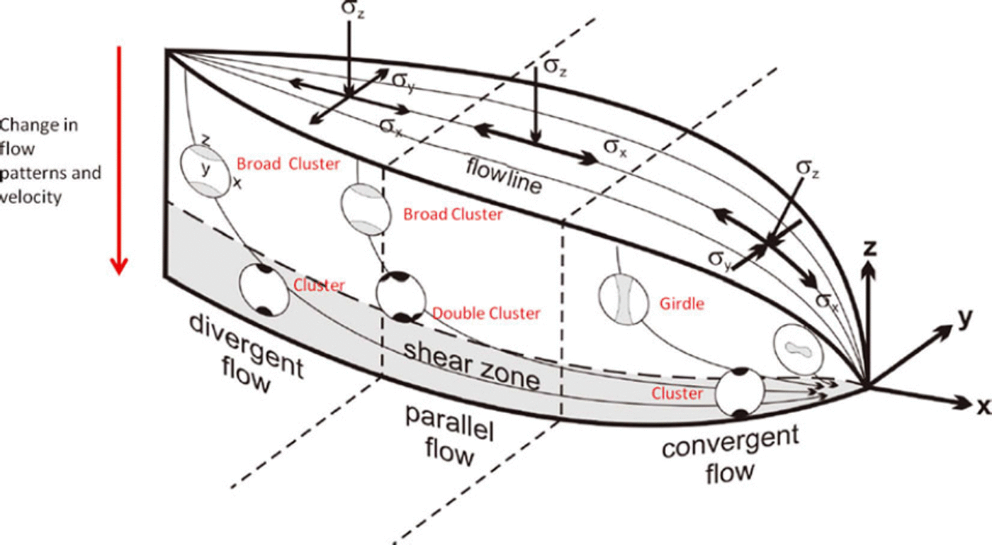
Fig. 2. Predictions of ice crystal fabric in an ice stream. Three flow regimes are indicated (divergent, parallel and convergent flow) and the corresponding stress (σ) regimes are indicated above. A basal shear zone consistently shows a cluster or solid-cone distribution in c-axes, although a double cluster is predicted in the region of parallel flow. There is a transition from a cluster model to a girdle model as the flow becomes convergent. Modified from Reference AzumaAzuma (1994).
Another mechanism that is very effective in producing anisotropy is the alignment of cracks or melt films (Reference Kendall, Jolley, Barr, Walsh and KnipeKendall and others, 2007), which is sometime, referred to as a shape-preferred orientation (SPO). A material with an aligned set of cracks will behave as an effectively homogeneous but anisotropic medium as long as the seismic wavelength is much larger than the crack spacing. Aligned vertical cracks can be treated as an HTI medium. Depending on the wetting angle, melt films in glaciers can be ellipsoidal in shape (Reference MaderMader, 1992) and, if aligned, will be very effective in producing anisotropy. Alternatively, the alignment of larger cracks and fissures will also be effective in generating a seismic anisotropy. Distinguishing between a more intrinsic anisotropy due to ice crystal alignment and a more extrinsic mechanism due to crack alignment can be challenging and requires datasets with very good angular coverage in ray paths (Reference Verdon, Kendall and WustefeldVerdon and others, 2009).
In Situ Measurements of Ice Anisotropy
There are many seismic methods for studying elastic anisotropy using both body waves and surface waves (e.g. Reference Brisbourne, Stuart and KendallBrisbourne and others, 1999; Reference Kendall, Jolley, Barr, Walsh and KnipeKendall and others, 2007). A potential problem with P-wave studies is the trade-off between heterogeneity along the ray paths and anisotropy. Icequakes are very efficient in generating shear waves, and with accurate source locations shear-wave anisotropy along the ray path can be studied. Measurements from multiple ray paths can be then used to constrain the style of anisotropy (e.g. Reference Verdon, Kendall and WustefeldVerdon and others, 2009).
In a series of remarkable Antarctic seismic experiments in the late 1960s and early 1970s our knowledge of ice anisotropy advanced significantly (Reference BentleyBentley, 1975). Reference AcharyaAcharya (1972) used surface wave dispersion measurements to estimate 8–10% shear-wave anisotropy in the ice cap at Byrd Land. He attributed this to near-surface layering in the upper few hundred metres of ice (for a description of the mechanism see Reference BackusBackus, 1962). Reference RobinsonRobinson (1968) considered body and surface wave data across the polar plateau and the Ross Ice Shelf, showing that the near-surface velocity of the plateau was isotropic whilst the Ross Ice Shelf exhibited nearly 20% P-wave anisotropy. In a series of experiments, Reference Bentley and CraryBentley (1971) observed azimuthal variations of P-waves from refraction and wide-angle reflection data, which he related to the CPO of ice crystals. He also observed shear-wave splitting in converted P–S reflections. In an earlier refraction experiment, Reference Bentley and OdishawBentley (1964) observed nearly 30 ms of shear-wave splitting (birefringence) between vertically (Sv) and horizontally (Sh) polarized shear waves that propagated for >6.5 s.
The connection between ice fabric and seismic velocities was better established using ultrasonic measurements in a deep borehole at Byrd Station (Reference BentleyBentley, 1972). This work showed P-wave anisotropy at depths greater than 400 m, which increased dramatically at depths greater than 1200 m, but then decreased again below 1800 m. A notable conclusion from this work is the depth-dependent variations in the symmetry of the ice anisotropy, where near-vertical c-axes orientation was inferred in the deeper parts of the ice sheets but a double cluster or asymmetry in c-axes clustering was observed at intermediate depths. Reference Anandakrishnan, Fitzpatrick, Alley, Gow and MeeseAnandakrishnan and others (1994) used both compressional and shear-wave transducers to study c-axes alignment in ice core from Greenland. They showed a decrease with depth in the solid-cone angle the c-axes make to the vertical, but also noted some asymmetry in the clustering. Most recently Reference Gusmeroli, Pettit, Kennedy and RitzGusmeroli and others (2012) have established a theoretical basis for using borehole sonic logging to assess the fabric of polycrystalline glacial ice. Cumulatively, these studies have shown that ice anisotropy may vary both laterally and with depth in ice masses.
The Icequake Dataset
The microseismic dataset was collected in the austral summer of 2008/09 (between December 2008 and February 2009). Ten stations of high-frequency (1 kHz) three-component geophones were deployed in two arrays of five stations (Reference Pritchard, Brisbourne, King, Gudmundsson and SmithPritchard and others, 2011). The horizontal components were orientated parallel (north component) and perpendicular (east component) to the ice-flow direction. Each instrument was buried at 1 m depth to reduce ambient noise and increase coupling by lying below fresh snow.
Array locations were guided by the results of previous reflection and microseismic surveys (Reference SmithSmith, 1997a,Reference Smithb; Reference SmithSmith, 2006). The south array was sited over an area of harder bed, where basal sliding occurs, whereas the north array was sited above an area of deformable sediment (Reference SmithSmith, 2006). Data from the south array were used in this study as it recorded many more events due to the array being over a high-friction ‘sticky spot’ (Reference SmithSmith, 2006). Here we analyse 250 events recorded by all five stations over the course of 1 day.
Only events with high signal-to-noise ratios (SNRs) are analysed, and acceptable events had clear P-wave arrivals on at least four stations. In many cases, the fast and slow shear waves were clearly visible on the unrotated seismograms, presumably due to the orientation of the horizontal components with the flow direction. Figure 3 shows an example of a typical high-SNR event.

Fig. 3. An example of a typical icequake recorded at station 1. The P-wave (P), fast shear wave (S1) and slow shear wave (S2) are marked. The S-P travel time used to locate the event is marked t S-P and the delay time between the fast and slow shear wave is marked St.
The events were located using a nonlinear inversion of P- and S-wave travel times (HYPO2000; Reference KleinKlein, 2000). Owing to a lack of knowledge of the velocity structure of the Rutford ice sheet, a homogeneous isotropic model was assumed. Based on Reference RothlisbergerRöthlisberger (1972), the P-wave velocity (V p) was assumed to be 3.60 kms-1 and S-wave velocity (V s) 1.85 kms-1, giving a Vp/Vs ratio of 1.95. The travel time of the earliest arriving S-wave signal was used in the inversion. Not all events could be located due to intermittent failure of one of the stations. The total number of successfully located events was 41 (Fig. 4), most of which were located close to the base of the ice, estimated from radar imaging (Reference KingKing, 2009).
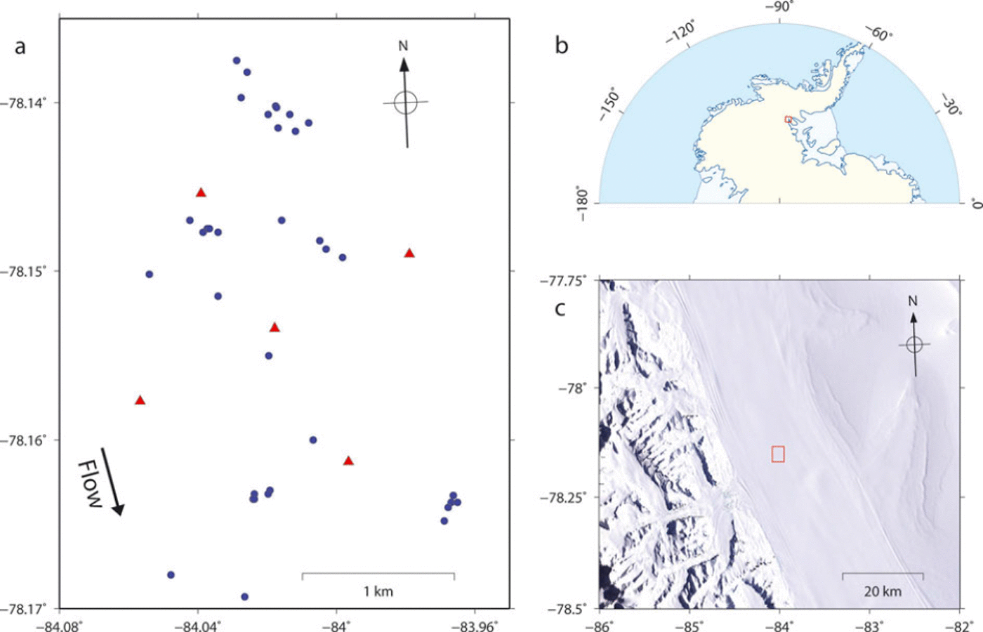
Fig. 4. Locations of seismic stations, icequake epicentres and the microseismic experiment. (a) Epicentres are shown in blue and stations in red; the arrow indicates the flow direction of the ice stream. (b) The red square indicates the location of the experiment. (c) The red square indicates the location of the experiment on a map showing the surface elevation of Rutford Ice Stream (natural colour Landsat image). The flow direction of the ice stream is ∼165°.
Clusters of events are revealed by similar S-P travel times and waveforms, showing that events occur repeatedly at the same locations throughout the day (Fig. 4). The error in estimated depth of the events is much larger than lateral location errors (hundreds versus tens of metres). Location errors are most likely due to a lack of detailed knowledge of the velocity structure of the ice stream. Preliminary analysis of focal mechanisms derived from first motions suggests low-angle thrust mechanisms, consistent with stick-slip stress release at the base of the ice stream.
Shear-Wave Splitting Analysis
For a given event, shear-wave splitting is measured for each station using the approach of Reference Wuestefeld, Al-Harrasi, Verdon, Wookey and KendallWuestefeld and others (2010). The analysis estimates the splitting parameters (which is the polarization of the fast shear wave) and δ t (the time delay between the fast and slow shear waves). A grid search over all possible fast shear-wave polarizations and delay times (up to 100 ms) is used to find the splitting parameters that best linearize the particle motion, thus removing the effects of the anisotropy. In practice, the grid search minimizes the second eigenvalue of the covariance matrix of the S-wave signal recorded on the two horizontal components. The analysis is done on 100 windows around the S-wave, and a cluster analysis is used to assess the stability of the solution (Reference Teanby, Van der Baan and KendallTeanby and others, 2004). A statistical f test is used to assess the errors in the estimates of the splitting parameters. The analysis also estimates the initial S-wave polarization at the source. So-called ‘null’ results occur when the medium is isotropic or when the initial source polarization is aligned with the fast or slow shear-wave polarization. Inconclusive results and high error estimates occur when the data are noisy.
Figure 5 shows an example of a shear-wave splitting measurement on an icequake. The clear separation between the fast and slow shear waves is apparent on the unrotated data (Fig. 3), which leads to an x-shaped S-wave particle motion. Such an observation is very unusual in conventional earthquake data. A more familiar elliptical particle motion is observed when the delay time (δt) is less than the dominant period of the S-waves (e.g. Reference Wuestefeld, Al-Harrasi, Verdon, Wookey and KendallWuestefeld and others, 2010). The splitting analysis linearizes the particle motion and minimizes the S-wave energy on the component aligned perpendicular to the initial S-wave polarization.

Fig. 5. An example of a shear-wave splitting measurement made on the icequake record shown in Figure 3. (a) The fast and slow shear waves before and after correcting for the shear-wave splitting. (b) The shear-wave particle motion before and after determining the shear-wave splitting parameters that best linearize the particle motion.
With surface sensors, the splitting analysis can only be performed when the ray-path direction is <45° to the vertical (i.e. within the shear-wave window). At greater angles, free-surface effects can generate elliptical particle motion in the S-wave arrivals (Reference Booth and CrampinBooth and Crampin, 1985).
The analysis produces 111 reliable shear-wave splitting measurements from the 41 events that were considered. Events with errors in exceeding 10° were discarded, as were those with delay time (δt) errors exceeding 10%. The average delay time for the dataset is 35 ms, but these range from 2 ms to a maximum of 80 ms. Figure 6 shows that the fast shear-wave polarizations cluster around the direction perpendicular to the flow of the ice stream, while the initial source polarizations cluster around the direction of ice flow. It should be noted that a source polarization that is exactly perpendicular to the fast shear-wave polarization would result in a ‘null’ measurement. The more northerly event station pairs gave generally better results due to the higher SNR at the more northerly stations.
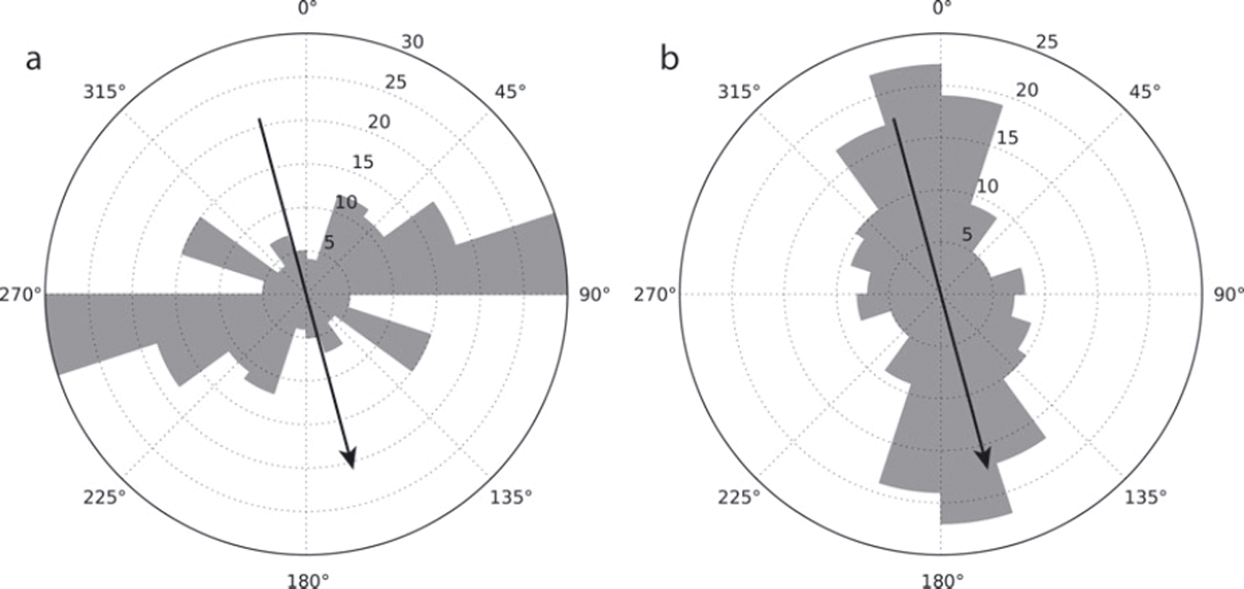
Fig. 6. Rose diagrams for (a) fast shear polarizations and (b) initial source polarizations for the entire set of shear-wave splitting measurements. The black arrow indicates the ice-flow direction.
Interpretation and Discussion
Figure 7 shows the splitting results plotted in map view at the surface projection of the midpoint between the source and receiver. The diagram shows that the dominant fast shear-wave polarization (Φ) is oriented perpendicular to the ice-stream flow direction. It also shows the variability in the magnitude of the splitting (δt) but does not take into account variations in ray-path directions. A better representation of the variation in splitting with ray azimuth and inclination is shown on an upper hemisphere projection of the results (Fig. 8a). To aid interpretation of the results and as the station array is located within the region of convergent flow on the ice stream, we consider each result as a sample of the same flow regime but along varying ray directions.

Fig. 7. A map view of the shear-wave splitting results. The events (blue circles) and stations (red triangles) are marked and the splitting measurement is plotted at the midpoint of the ray path (dashed line). The tick length is proportional to the magnitude of the splitting, and the tick orientation shows the polarization of the fast shear wave. The flow direction of the ice stream is 1658.
We can rule out a simple VTI model of ice anisotropy as there is significant splitting in the vertical directions and there is clearly significant variation in the magnitude of the splitting with ray azimuth (cf. Figs 1 and 8a). This means that a cluster or solid-cone model alone does not fit the data. Based on the predictions of Reference AzumaAzuma (1994) this is perhaps not surprising. In order to understand these variations in delay times and fast polarization directions between stations, we employ the shear-wave splitting inversion technique proposed by Reference Verdon, Kendall and WustefeldVerdon and others (2009). We assume a physical model for the anisotropy that is based on a single set of vertically aligned cracks superimposed on an intrinsically VTI medium, which yields an effectively orthorhombic medium. We then seek to find the model parameters that best fit our observations. This method finds the fracture parameters (strike and density) that best fit the observations; for more detail, see Reference Verdon, Kendall and WustefeldVerdon and others (2009) and Reference Wuestefeld, Verdon, Kendall, Rutledge, Clarke and WookeyWuestefeld and others (2011).

Fig. 8. (a) The shear-wave splitting results plotted on an upper-hemisphere projection. Vertical ray paths plot at the centre, and horizontally propagating rays would plot at the edge. The tick colour and length is proportional to the magnitude of the splitting, and its orientation shows the polarization of the fast shear wave. (b) Same as (a) but also showing the HTI model that best fits the shear-wave splitting measurements. This shows the orientation and magnitude of splitting for the girdle model that best explains the data. Black ticks show the orientation of the fast shear-wave polarization, and their length is proportional to the splitting. Colour scale indicates the magnitude of the anisotropy. (c) Same as (a) but also showing the orthorhombic model that best fits the shear-wave splitting measurements. The data are inverted for a model with vertically aligned cracks superimposed on a model with VTI symmetry. Black ticks show the orientation of the fast shear-wave polarization predicted by the model, and their length is proportional to the splitting. Ticks with a white outline are the fast shear-wave polarizations for the observations. Colour scale indicates the magnitude of the anisotropy.
A girdle model of ice anisotropy, where the Ih crystal c-axes lie in a vertical plane normal to the flow direction, is not inconsistent with the observations. This is in agreement with the predictions of Reference AzumaAzuma (1994), as the microseismic survey is located close to the grounding line and therefore the ice-stream outlet, meaning that the flow regime is likely convergent. Figure 8b shows the best-fitting girdle model, assuming a hexagonal symmetry with the symmetry axis (a-axes clustering) oriented horizontally in the flow direction. It predicts the a-axis to be oriented at 162 ±5° (the ice-stream flow direction is 165°N).
Finally, we consider a model where the anisotropy is due to vertically aligned cracks or melt films (hereafter simply referred to as cracks as it is not possible to distinguish between these mechanisms without more detailed analysis of the data). As described above, we invert the data for a model with a background VTI symmetry that it superimposed with an HTI symmetry. The best-fitting model is shown in Figure 8c. The VTI component could be attributed to a solid-cone or cluster model, and the HTI component is due to orientated cracks. The VTI component is not well constrained as there is a lack of near-horizontal ray paths. In contrast, the HTI component is well constrained and is best fit by a crack set with a strike of 55 ± 10° (or 1450; i.e. ∼15° from the normal to flow direction) and a fracture density of 0.046 (crack density = Nr 3 /V, where N is the number of cracks in a volume V and r is the average crack radius, assuming penny-shaped cracks; Reference HudsonHudson, 1981). For the best-fitting model, the maximum contribution to the anisotropy from aligned cracks is ∼4%.
In an attempt to assess which models best fit the data, we calculate the residual misfit for both the shear-wave polarizations and the splitting magnitudes. We compute modelled shear-wave splitting parameters for each azimuth and inclination present in the observed dataset. We compute the root-mean-square (rms) misfit for polarization direction and magnitude separately and normalize each by their minimum values before summing them to give an overall misfit. The different normalization factors for each model make a direct comparison of the combined misfit difficult; however, comparisons can be made for the individual misfit values. The VTI model gives the worst fit to the data. Based on polarizations (f), the HTI models (either the girdle fabric or crack-induced anisotropy) fit the data better than the VTI or VTI+ HTI models. In contrast, based on misfit in splitting magnitudes (dt), the VTI +HTI mechanism is the best-fitting model. Without further data it is difficult to discriminate any further between models. Ideally, one would combine both misfit calculations (i.e. both <p and δt), but the relative weighting for each is a bit arbitrary.
Without more data it is difficult to discriminate between the girdle model and the crack model as an explanation for the HTI component of the anisotropy. It is conceivable that both mechanisms are at play, but perhaps with different intensities at different depths or with varying distance from the flanks of the ice stream. The crack hypothesis would require a dominant alignment in the direction perpendicular to the direction of ice-stream flow.
There are a number of steps that could be taken to improve certainty in the best-fitting model of ice anisotropy. Analysis of P-wave anisotropy would be complementary – perhaps using controlled-source seismic refraction and reflection experiments. Azimuthal variations in P-wave velocities (e.g. Reference Bentley and CraryBentley 1971) and/or amplitudes (Reference Hall and KendallHall and Kendall, 2003) will be indicative of non-VTI models. Alternatively, non-hyperbolic moveout in seismic reflections is indicative of VTI anisotropy (e.g. Reference Van der Baan and KendallVan der Baan and Kendall, 2002). Finally, the combined analysis of body wave and surface wave data helps constrain the spatial patterns and mechanisms of anisotropy (e.g. Reference Brisbourne, Stuart and KendallBrisbourne and others, 1999; Reference Snyder and BrunetonSnyder and Bruneton, 2007).
Ideally a denser array of sensors is needed to look at lateral variations across the ice stream. This would allow better testing of the model of Reference AzumaAzuma (1994). It would also be useful to have some control on depth variability in the anisotropy. Unfortunately, the icequakes at Rutford Ice Stream seem to be confined to the ice bed. Another approach is to use borehole data. Three-component borehole sensors can be deployed in an array to record icequakes, as is commonly used in monitoring hydraulic stimulation of petroleum reservoirs (e.g. Reference Wuestefeld, Verdon, Kendall, Rutledge, Clarke and WookeyWuestefeld and others, 2011). This avoids problems with the more attenuative near-surface and removes issues of the shear-wave window (i.e. there is no free-surface effect). Therefore it is possible to record ray paths closer to horizontal and better discriminate between models. Finally, borehole sensors and a shear-wave surface source would also help constrain depth variations in ice anisotropy.
Ice streams sometimes change in speed and orientation. Identifying these variations may provide important first indications of possible ice-stream disintegration and acceleration, as has recently occurred on the Larsen B ice shelf. After break-up, Reference Scambos, Bohlander, Shuman and SkvarcaScambos and others (2004) identified changes in glacier velocity using GPS. However, any evidence of temporal variations in shear-wave splitting could be used to track such changes closer to real time and, more importantly, determine how quickly rheology responds to such change. Stress changes associated with hydraulic stimulation have been documented in both petroleum (Reference Wuestefeld, Verdon, Kendall, Rutledge, Clarke and WookeyWuestefeld and others, 2011) and volcanic settings (Reference Johnson, Prejean, Savage and TownendJohnson and others, 2010) using observations of shear-wave splitting.
Conclusions
Shear-wave splitting has been measured in 41 icequakes from the base of Rutford Ice Stream recorded by an array of five seismometers deployed at the surface near the grounding line. The events are located using S-P travel time residuals and are consistent with a stick–slip mechanism. The events cluster in regions, suggesting the locations of points where the friction between the ice and bedrock is highest.
We observe large variations in the magnitude of the shear-wave splitting (2–80 ms), and the polarization of the fast shear wave is dominantly orthogonal to the flow of the ice stream. The average magnitude of the shear-wave anisotropy for the entire thickness of the sheet is a maximum of 6% (the anisotropy may be higher if confined to more localized regions).
We consider three causes of the anisotropy. The first is a solid-cone or cluster model, where the c-axes orient in a sub-vertical cone. This produces a VTI symmetry. Previous results have shown that the angle the cone makes with the vertical should decrease as the confining pressure increases. This model predicts very little shear-wave splitting for vertical wave propagation, which is inconsistent with the observations. We therefore conclude that this model alone cannot explain the results. We next consider the girdle model where the c-axes align in a vertical plane perpendicular to the ice-stream flow, with a concentration of a-axes parallel to the flow direction. This produces an HTI symmetry. This model explains the observations for sub-vertical ray paths. We finally consider a model that is a combination of VTI and HTI symmetry (i.e. an orthorhombic symmetry). With the data available it is difficult to constrain the VTI component of the anisotropy and, as such, both HTI and orthorhombic models are viable.
There are two possible explanations for a model with both a VTI and an HTI component. The first is a cluster (solid-cone) model with a set of vertically oriented cracks aligned roughly perpendicular to the flow direction. Such cracks may be in response to undulations in bedrock topography or be due to much smaller melt films that are aligned by the stress field. Alternatively, the composite model may be due to the accrued anisotropy through a cluster model near the ice bed and a girdle model in the upper parts of the ice stream. Such a model is consistent with the predictions of Reference AzumaAzuma (1994). Reference BentleyBentley (1972) observed vertical variations in the style and magnitude of ice anisotropy near the Byrd Station drillhole, and further support comes from petrofabric analysis of core data (Reference Obbard and BakerObbard and Baker, 2007).
Future icequake monitoring experiments with both surface and borehole sensors would provide a detailed picture of vertical variations in ice anisotropy, which would be invaluable for calibrating ice-flow models that include anisotropic rheologies. We have presented the first documented observation of shear-wave splitting in icequakes, and the initial results suggest that this is a fruitful means of better quantifying in situ ice anisotropy.
Acknowledgements
We thank editors Matt King and Bernd Kulessa for handling the manuscript and acknowledge the helpful comments of two reviewers, which improved the manuscript. SEIS-UK is acknowledged for the loan of equipment (NERC Geophysical Equipment Facility, Loan No. 852) and we thank BAS Operations and Chris Griffiths for field support. This study is part of the BAS Polar Science for Planet Earth Programme and was funded by the Natural Environment Research Council (NE/B502287/1). Rachel Obbard is acknowledged for her EBSD results and advice on ice crystal fabrics.


