


1. Introduction
Since the seminal pipe flow experiments of Osborne Reynolds (Reynolds Reference Reynolds1883), experiments have been widely designed and used to study fluid flow (Tropea, Yarin & Foss Reference Tropea, Yarin and Foss2007). The recent development of state-of-the-art measurement techniques allows the investigation of flow fields at high spatio-temporal resolution (e.g. Partridge, Lefauve & Dalziel Reference Partridge, Lefauve and Dalziel2019). However, experimentalists often face the challenge of accurately measuring flow structures across a wide range of scales, particularly in turbulent flows. Moreover, latent flow variables, such as the pressure field, can rarely be measured. To complement experiments, numerical simulations are widely used, often affording better resolution and the full set of flow variables. However, simulations remain idealised models subject to computational limits. These limitations make them challenging to deploy in regions of parameter space appropriate to environmental or industrial applications, as well as in realistic geometries with non-trivial boundary conditions.
Recent advances in machine learning have stimulated new efforts in fluid mechanics (Vinuesa, Brunton & McKeon Reference Vinuesa, Brunton and McKeon2023), with one application being the reconstruction of flow fields from limited observations (Fukami, Fukagata & Taira Reference Fukami, Fukagata and Taira2019; Raissi, Yazdani & Karniadakis Reference Raissi, Yazdani and Karniadakis2020; Wang et al. Reference Wang, Li, Liu, Wu, Hao, Zhang and He2022b). Among the available tools, physics-informed neural networks (PINNs) (Raissi, Perdikaris & Karniadakis Reference Raissi, Perdikaris and Karniadakis2019) hold particular promise. The idea behind a PINN is to impose physical laws on a neural network fed with observations. This allows the model to super-resolve the flow in space and time, to remove spurious noise, and to predict unmeasured (latent) variables such as the pressure (Raissi et al. Reference Raissi, Perdikaris and Karniadakis2019). Consequently, PINNs have recently received increasing attention within the experimental fluid mechanics community (Cai et al. Reference Cai, Wang, Fuest, Jeon, Gray and Karniadakis2021; Wang, Liu & Wang Reference Wang, Liu and Wang2022a; Fan et al. Reference Fan, Xu, Wang and Wang2023), but the reconstruction of three-dimensional data acquired in density-stratified flows has remained a challenge, owing to the wide spatial and temporal scales and the scarcity of high-quality data in the experiment.
In this paper, we demonstrate the potential of a PINN to augment state-of-the-art experimental data and reveal important new physical insights into density-stratified flows. For this purpose, we use the canonical stratified inclined duct (SID) experiment (Meyer & Linden Reference Meyer and Linden2014) sustaining a salt-stratified shear flow in a long tilted duct. The PINN is fed datasets comprising the time-resolved, three-component velocity field and density field measured simultaneously in a three-dimensional volume by a scanning technique. We focus on experiments in the Holmboe wave (HW) regime, as these interfacial waves are important precursors of three-dimensional turbulence in environmental flows, e.g. between strongly stratified layers in the ocean (Kaminski et al. Reference Kaminski, D'Asaro, Shcherbina and Harcourt2021; Kawaguchi et al. Reference Kawaguchi2022).
In the remainder of this paper, we describe the datasets, the PINN and the validation in § 2, and our results in § 3. We demonstrate the improvement in signal-to-noise ratio in § 3.1, in the detection of weak but important coherent structures in § 3.2, in the accuracy of energy budgets and quantification of scalar mixing in § 3.3. We also show in § 3.4 that the latent pressure field revealed by the PINN is key to explain asymmetric HWs in SID flow. Finally, we conclude in § 4.
2. Methodology
2.1. The SID dataset
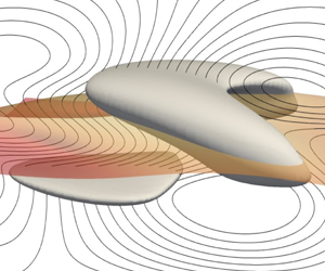
The data were collected in the SID facility (sketched in figure 1), where two salt solutions with density  $\rho _0\pm \Delta \rho /2$ are exchanged through a long duct of square cross-section tilted at a shallow angle $\theta$. Importantly, the volumetric, three-component velocity and density fields are collected through a continuous back-and-forth scanning of a streamwise ( $x$) – vertical ( $z$) laser sheet across the spanwise ( $\kern 1.5pt y$) direction, as introduced in Partridge et al. (Reference Partridge, Lefauve and Dalziel2019). Figure 1 shows how $n_y$ successive planar measurements of laser-induced fluorescence (LIF, for density) and stereo particle image velocimetry (sPIV, for velocity) captured over a short time $\Delta t$ are aggregated to yield $n_t$ ‘near-instantaneous’ volumes. The typical processed dataset has $(n_x,n_y,n_z,n_t) \approx (400,35,80,250)$ points, noting that the spatial resolution in $x$ and $z$ is identical but is approximately two to three times higher (better) than that along $y$.
$y$.
The SID set-up and dataset. Each volume is constructed by aggregating  $n_y$ planes (closely spaced dots) obtained by scanning across the duct over time $\Delta t$.

All data are made non-dimensional with the following scales. For the spatial coordinates we use the half-duct height  $H^*/2=22.5$ mm. For the velocity we use half the fixed peak-to-peak ‘buoyancy velocity’ scale $U^*/2 \equiv \sqrt {g^\prime H^*}$ (where $g^\prime =g\Delta \rho /\rho _0$ is the reduced gravity chosen for the experiment), leading to velocities being approximately bounded by ${\pm }1$. This means time is non-dimensionalised by the advective unit $H^*/U^*$, yielding the Reynolds number $Re = H^* U^\ast/(4\nu)$, where $\nu$ is the kinematic viscosity of water. The Prandtl number is $Pr=\nu /\kappa \approx 700$, where $\kappa$ is the molecular diffusivity of salt. For the density field (its deviation from the neutral level $\rho _0$, i.e. the buoyancy) we use half the maximum jump $\Delta \rho /2$, which yields the fixed bulk Richardson number $Ri = (g^\prime /2) (H^\ast /2)/(U^{\ast }/2)^2=1/4$. The data can be downloaded from Lefauve, Partridge & Linden (Reference Lefauve, Partridge and Linden2019a). We focus on comparing two typical HW datasets: H1 featuring a double-mode, symmetric HW at $(Re,\theta )=(1455,1^\circ )$; and H4, featuring a single-mode, asymmetric HW at $(Re,\theta )=(438,5^\circ )$ studied in detail in Lefauve et al. (Reference Lefauve, Partridge, Zhou, Dalziel, Caulfield and Linden2018).
2.2. The PINN
The PINN used to augment the time-dependent, three-dimensional, multi-scale data is sketched in figure 2. A fully connected deep neural network is set up using the spatial  $\boldsymbol {x}=(x,y,z)$ and temporal $t$ coordinates of the flow domain as the inputs, and the corresponding velocity $\boldsymbol {u}=(u,v,w)$, density $\rho$, and pressure $p$ as the outputs. The network is composed of 14 layers with an increasing number of artificial neurons ([ $64\times 4$, $128\times 3$, $256\times 4$, $512\times 3$]). A sensitivity analysis on the network architectures was conducted to ensure sufficient complexity of the network to capture the nonlinear dynamics of the flow. The outputs of each layer $\boldsymbol {n}_k$ are computed by a nonlinear transformation of the previous layer $\boldsymbol {n}_{k-1}$ following the basic ‘neuron’ $\boldsymbol {n}_k=\boldsymbol {\sigma }(\boldsymbol {w}^T_{k-1}\boldsymbol {n}_{k-1}+\boldsymbol {b}_{k-1})$, where $\boldsymbol {b}_{k-1}$ and $\boldsymbol {w}^T_{k-1}$ are the bias vectors and weight matrices of layer $k-1$. To introduce nonlinearity and overcome the potential vanishing gradient of deep networks, we use a Swish activation function $\boldsymbol {\sigma }$ for all the hidden layers (Ramachandran, Zoph & Le Reference Ramachandran, Zoph and Le2017).
Schematics of the PINN. The output variables  $(\boldsymbol {u},\rho,p)$ (in yellow) are predicted from the input variables $(\boldsymbol {x},t)$ (in orange) subject to physical constraints (blue) and experimental observations (in red).

The outputs  $\boldsymbol {u}$ and $\rho$ are compared with experimental data, $\boldsymbol {u}_O$ and $\rho _O$ (i.e. observations), to obtain the absolute mean error loss function $\mathcal {L}_O$ (in red in figure 2). The spatial and temporal derivatives of $\boldsymbol {u}$, $\rho$ and $p$ are computed at every sampling point using automatic differentiation (Baydin et al. Reference Baydin, Pearlmutter, Radul and Siskind2018) (in green). To impose the physical constraints, the derivatives are substituted into the governing mass, momentum, and density scalar equations, corresponding to loss functions $\mathcal {L}_{E1}$, $\mathcal {L}_{E2}$, $\mathcal {L}_{E3}$, respectively (in blue). We also impose the boundary conditions through $\mathcal {L}_{B}$ (no-slip $\boldsymbol {u}=0$, and no-flux $\partial _y\rho =0, \partial _z\rho =0$ at the four walls $y=\pm 1, z=\pm 1$, respectively).
Combining these constraints, we define the total loss function
 \begin{equation} \mathcal{L}_{tot}=\frac{\lambda_E}{N_E}\sum_{j=1}^{N_E}\sum_{i=1}^3\mathcal{L}_{Ei}^j+ \frac{\lambda_B}{N_B}\sum_{j=1}^{N_B}\mathcal{L}_{B}^j+ \frac{\lambda_O}{N_O}\sum_{j=1}^{N_O}\mathcal{L}_{O}^j, \end{equation}
where  $\lambda _E$, $\lambda _B$ and $\lambda _O$ are weight coefficients for the governing equation, boundary condition and observation losses, respectively (of recent work, the formulation in Calicchia et al. (Reference Calicchia, Mittal, Seo and Ni2023) is perhaps closest to ours here with one difference that we impose boundary conditions appropriate for solid walls). The number of training samples are defined as $N_E$, $N_B$ and $N_O$ for the equations, boundaries and observations, respectively. Here $N_O=10^7$ for H1 and $N_O=3\times 10^7$ for H4 (noting it depends on the resolution of the data), $N_B=4\times 10^6$ and $N_E=10^7$. Through optimising the loss function (2.1), the governing equations and boundary conditions are required to be satisfied at the physical training points, enabling PINN to gain information beyond the experimental observations, thus facilitating super-resolution. The neural network is trained to seek the optimal parameters using the ADAM algorithm (Kingma & Ba Reference Kingma and Ba2014) to minimise the total loss $\mathcal {L}_{tot}$. To enhance convergence of the training procedure, we adopt exponentially decaying optimiser steps with training taking approximately $100$ GPU hours on a NVIDIA A100 GPU.
A key strength of this PINN is its natural ability to reconstruct truly instantaneous three-dimensional flow fields by overcoming the spanwise distortion of the near-instantaneous data acquired by scanning (as also attempted by Knutsen et al. Reference Knutsen, Baj, Lawson, Bodenschatz, Dawson and Worth2020; Zigunov et al. Reference Zigunov, Seckin, Huss, Eggart and Alvi2023). This is done simply by feeding the  $n_y$ successive snapshots $(\boldsymbol {u},\rho )(x,y_i,z,t_i)$, taken during each alternating forward and backward scan (see figure 1), at times $t_i$ equally spaced by $\Delta t/n_y$, where $(\Delta t,n_y)=(2.29,39)$ for H1 and $(1.08,30)$ for H4. In addition to the realignment of the sampling data, the PINN constraints enforce a physically sensible nonlinear projection of scanned data toward the ground truth, resulting in a correction that is more accurate and reliable than any ad hoc kinematic correction.
2.3. Validation of PINN with DNS
To validate the performance of the PINN in reconstructing SID flow, we apply it to a direct numerical simulation (DNS) at  $Pr=7$, representative of temperature stratification in water (it is very costly to resolve DNS with $Pr=700$ relevant for salt stratification). The DNS is run with periodic streamwise boundary conditions, resulting in a stationary Kelvin–Helmholtz instability (also observed in experiments at this $Pr$), rather than a travelling Holmboe wave instability. To mimic the imperfections of our experimental data, we trained a 10-layer PINN (with $[64\times 4,128\times 4,256\times 2]$ neurons) after equally spaced downsampling the velocities and density DNS data to a spatial resolution ( $(n_x,n_y,n_z)=(150,31,61)$), adding $5\,\%$ random noise and feeding $x$–
$x$– $z$ planes as if they were acquired by scanning along $y$. We find that the PINN faithfully reproduces the DNS results, with a point-wise error below $3\,\%$ in the vertical velocity $w$ and pressure $p$ (not used for training): see figure 3.
Validation of the PINN with a DNS: (a–c) vertical velocity  $w(x,y,z=0)$, and (d,e) pressure $p(x,y,z=0)$. Note the DNS ‘ground truth’ (a,d, note $u,v,\rho$ are not shown here); training sample (b) excluding the pressure; and PINN reconstruction (c,e).

3. Results
3.1. Improved quality of experimental data
We start by comparing flow snapshots and statistics of HWs in the raw experimental data with the PINN-reconstructed data. While neural networks approach a solution through continuous functions, here we show results with a spatial resolution typically twice that of the experimental data in the  $x$,
$x$,  $y$ and $z$ directions (note that higher resolutions are possible by increasing the sampling input points). Instantaneous volumes are also generated at a higher temporal resolution than acquired experimentally, namely at intervals $\Delta t=0.24$ (for H1) and $0.74$ (for H4), noting that we restrict our analysis to times $t\in [150\unicode{x2013}200]$ (for H1) and $t\in [150\unicode{x2013}300]$ (H4). Comparisons of the time-resolved H1 and H4 raw and PINN data are provided in supplementary movies 1–4 available at https://doi.org/10.1017/jfm.2024.49.
First, figure 4(a,b) shows a snapshot of the vertical velocity  $w(x,z)$ taken in the mid-plane $y=0$ and at time $t=283$ in H4. The large-scale HW structures of the experiment (figure 4a) are faithfully reconstructed by the PINN (figure 4b) with much less small-scale structure, which we identify as experimental noise, violating the physical constraints and increasing the loss in (2.1). This $w$ snapshot closely matches the ‘confined Holmboe instability’ mode predicted by Lefauve et al. (Reference Lefauve, Partridge, Zhou, Dalziel, Caulfield and Linden2018) (see their figure 9m) from a stability analysis of the mean flow in the same dataset H4. Such ‘clean’, noise-free augmented experimental data will improve the three-dimensional structure of HW as we will discuss in § 3.2.
Improvement of instantaneous snapshots: (a,b) vertical velocity  $w(x,y=0,z)$ in H4 at $t=283$, and (c–f) density just above the interface $\rho (x,y,z=0.1)$ in H1 at (c,d) $t=178.9$ (forward scan) and (e,f) $t=181.2$ (backward scan).

Second, figure 4(c–f) illustrates how the PINN is able to correct the inevitable distortion of experimental data along the spanwise, scanning direction (recall § 2.1 and figure 1), also clearly visible in supplementary movie 1. The top view shows a snapshot of the horizontal plane  $\rho (x,y)$ sampled at $z=0.1$ near the density interface of neutral density where $\langle \rho \rangle _{x,y,t} \approx 0$. Panels (c,e) show two successive volumes taken at time $t=178.9$ (forward scan) and $181.2$ (backwards scan) in flow H1, where the distortion is greatest (due to $\Delta t=2.3$ twice as large as in H4), while panels (d,f) show the respective instantaneous volumes output by the PINN. The original data make the peaks and troughs of this right-travelling HW mode appear alternatively slanted to the right during a forward scan, and to the left during a backward scan (see slanted black arrows). This distortion is successfully corrected by the PINN, which shows HWs propagating along $x$ with a phase plane normal to $x$ (straight arrows), as predicted by theory (Ducimetière et al. Reference Ducimetière, Gallaire, Lefauve and Caulfield2021).
Third, figure 5 compares the spatio-temporal diagrams of interface height  $\eta (x,t)$, defined as the vertical coordinate where $\rho (x,y=0,\eta,t)=0$. The characteristics showing the propagation of HWs in experiments (figures 5a,c) are largely consistent with the PINN results (figures 5b,d) but noteworthy differences exist. The determination of a density interface ( $\rho = 0$) is particularly subject to noise due to a low signal-to-noise ratio when the signal approaches zero. Here we see that the contours are rendered much less jagged by the PINN. The 10-fold increased temporal resolution in H1 ( $\Delta t=0.24$ vs 2.3) also allows a much clearer picture of the characteristics (figures 5c,d), which propagate in both directions, with sign of interference. By contrast, H4 has a single leftward propagating mode as a result of the density interface ( $\eta \approx -0.2$) being offset from the mid-point of the shear layer ( $u=0$ at $z\approx -0.1$), as explained by Lefauve et al. (Reference Lefauve, Partridge, Zhou, Dalziel, Caulfield and Linden2018). However, the reason behind this offset was not elucidated by experimental data alone, and will be elucidated by the pressure field in § 3.4.
Improvement of the spatio-temporal diagrams of the interface height  $\eta (x,t)$ for (a,b) H4 and (c,d) H1, capturing the characteristics of HW propagation.

Fourth, we quantify and elucidate the magnitude of the PINN correction through the root-mean-square difference  $d$ between the $\boldsymbol {u}$ and $\rho$ of the raw experiment and the reconstruction. We find $d=0.069$ for H1 and $d = 0.029$ for H4. We identify at least two sources contributing to $d$: (i) the noise in planar sPIV/LIF measurements, and (ii) the distortion of the volumes caused by scanning in $y$. As a baseline, we also compare a third, fully laminar dataset (L1) at $Re,\theta =(398, 2^\circ )$ (Lefauve, Partridge & Linden Reference Lefauve, Partridge and Linden2019b) having a PINN correction of $d=0.030$. In L1, $d$ is primarily attributed to (i), since this simple steady, stable flow renders (ii) negligible. The energy spectrum of L1 in Lefauve & Linden (Reference Lefauve and Linden2022) (their figure 4a) highlighted the presence of small-scale measurement noise. We are confident that cause (i) remains relatively unchanged in H1 and H4, resulting in $d$ being predominantly explained by (i) in H4, while the larger spanwise distortion (ii) must be invoked to explain the larger $d$ in H1, consistent with an increasing interface variation and a scanning time that is doubled in H1, as in figure 4(c–f).
3.2. Three-dimensional vortical structures of Holmboe waves
Previous studies of this HW dataset in SID flow revealed how, under increasing turbulence levels quantified by the product  $\theta Re$, the relatively weak three-dimensional Holmboe vortical structures evolve into pairs of counter-propagating turbulent hairpin vortices (Jiang et al. Reference Jiang, Lefauve, Dalziel and Linden2022). The particular morphology of these vortices conspires to entrain and stir fluid into the mixed interfacial region, elucidating a key mechanism for shear-driven mixing (Riley Reference Riley2022). However, Jiang et al. (Reference Jiang, Lefauve, Dalziel and Linden2022) alludes to limitations in the signal-to-noise ratio to accurately resolve the structure of the weakest nascent Holmboe vortices, as shown, e.g. in a visualisation of the $Q$-criterion in their figure 1.
Figure 6 shows how noise-free PINN data can uncover the vortex kinematics of this experimental HW in H4 by visualising an instantaneous  $Q=0.15$ isosurface (in grey), where $Q=(1/2)(\|\boldsymbol{\mathsf{W}}\|^2-\|\boldsymbol{\mathsf{E}}\|^2)$, using the Frobenius tensor norm of the strain rate $\boldsymbol{\mathsf{E}} =(1/2)(\boldsymbol \nabla \boldsymbol {u} + (\boldsymbol \nabla \boldsymbol {u})^{\rm T})$ and rotation rate $\boldsymbol{\mathsf{W}} =(1/2)(\boldsymbol \nabla \boldsymbol {u} - (\boldsymbol \nabla \boldsymbol {u})^{\rm T})$ (Hunt, Wray & Moin Reference Hunt, Wray and Moin1988). A density isopycnal surface just above the density interface is superposed, with yellow to red shading denoting its vertical position. The unsmoothed experiment data (figure 6a) are highly fragmented rendering these weak individual vortices unrecognisable. A similar noise pattern is observed in the fully laminar dataset L1, not shown here, confirming its unphysical nature. The PINN data (figure 6b) effectively filters out the noise, allowing us to analyse the vortex kinematics. Here, we show for the first time well-organised interfacial and $\varLambda$-like vortices in Q on either side of the isopycnal surface, corresponding to the coherence of nonlinear HWs in high- $Pr$ experiments.
Three-dimensional vortex and isopycnal surfaces in H4 at  $t=283$: (a) exp. vs (b) PINN. The grey isosurfaces show $Q=0.15$, while the colours show the isopycnal $\rho =-0.85$ and its vertical position $z \in [-0.2,0.2]$. The two black lines are the isopcynals $\rho =-0.85$ and $\rho =0$ in the mid-plane $y=0$.

The interfacial vortices are flat and appear to be formed when new wave crests appear (see left side of figure 6b), acting to lift and drop the interfaces, as the HW propagates (in this case, as a single left-going mode). These vortices play an inherent role in the formation and maintenance of the waves. As the linear HWs amplify and transition into the nonlinear regime (right side of figure 6b), a  $\varLambda$-shaped vortex, similar to those in transitional boundary layer (Jiang et al. Reference Jiang, Lee, Chen, Smith and Linden2020), is formed as vorticity is concentrated near the top of larger-amplitude isopycnal crests. This vortex may eject wisps of relatively mixed fluid at the interface (low $|\rho |$) up into the unmixed region (high $|\rho |$), leading to the upward deflection of isopycnals. This locally ‘anti-diffusive’ process is an example of scouring-type mixing typical of HWs (Salehipour, Caulfield & Peltier Reference Salehipour, Caulfield and Peltier2016; Caulfield Reference Caulfield2021) and allows a density interface to remain sharp. This $\varLambda$-shape vortex causes the distance between the $\rho =-0.85$ and $0$ isopycnals (the two black lines) to increase, indicating enhanced mixing in this region.
These findings confirm the hypothesis of Jiang et al. (Reference Jiang, Lefauve, Dalziel and Linden2022) and provide additional evidence for the existence of  $\varLambda$-vortices in HW experiments. While interfacial waves are generated during the initiation of a wave crest, the $\varLambda$-vortices emerge once the crest matures, playing a role in maintaining the sharpness of the interface. Similar $\varLambda$-vortices have also been observed in more idealised DNS of sheared turbulence at $Pr=1$ (Watanabe et al. Reference Watanabe, Riley, Nagata, Matsuda and Onishi2019), proving their relevance beyond the SID geometry and the importance of correctly identifying these coherent structures in experimental data, especially in parameter regimes currently inaccessible to DNS, as is the case here at $Pr=700$.
3.3. Energy budgets and mixing efficiency
The energetics of turbulent mixing in stratified flows is a major topic of research in environmental fluid mechanics (Caulfield Reference Caulfield2020; Dauxois et al. Reference Dauxois2021). The energy budgets of datasets H1 and H4 were investigated in Lefauve et al. (Reference Lefauve, Partridge and Linden2019b) and Lefauve & Linden (Reference Lefauve and Linden2022) but we will show that the PINN data can overcome limitations in spatial resolution (especially in  $y$), in the relatively low signal-to-noise ratio of perturbation variables in HWs, and other limitations inherent to calculating energetics from experiments.
Figure 7 shows four key terms in the budgets of turbulent kinetic energy (TKE)  $K^\prime =(1/2) (\boldsymbol {u}'\boldsymbol {\cdot } \boldsymbol {u}')$ and turbulent scalar variance (TSV) $K^\prime _\rho = (Ri/2) (\rho ')^2$, namely the production $P$ and dissipation $\epsilon$ of TKE, the buoyancy flux $B$ (exchanging energy between TKE and TSV) and the dissipation of TSV $\chi$, defined as in Lefauve & Linden (Reference Lefauve and Linden2022):
 \begin{align} P \equiv{-} \langle u'v'{\partial}_y \bar{u}+ u'w' {\partial}_z \bar{u}\rangle,\quad \epsilon \equiv \frac{2}{Re} \langle \|\boldsymbol{\mathsf{E}}'\|^2 \rangle,\quad B \equiv Ri \langle w' \rho'\rangle,\quad \chi \equiv \frac{Ri}{Re Pr}\langle |\nabla \rho'|^2\rangle, \end{align}
where fluctuations (prime variables) are computed around the  $x,t$ averages (overbars), as in $\phi '=\phi -\bar {\phi }$, and $\langle \, \rangle$ denotes averaging over $x,y$ and $t$ (but not $z$).
$z$).
Improved energy budgets in H1 and H4: vertical profiles of (a) production  $P$; (b) dissipation $\epsilon$; (c) buoyancy flux $B$; (d) scalar dissipation $\chi$; (e) mixing efficiency $\chi /\epsilon$, as defined in (3.1a–d). The blue and red dotted lines shows the mean density interface $\langle \rho \rangle =0$.

The vertical profiles of TKE production  $P(z)$ (figure 7a) show little difference between the PINN data (solid lines) and the experimental data (dashed lines), whether in H1 (blue) or H4 (red). We rationalise this by the fact that $P$ does not contain any derivatives of the velocity perturbations, and is thus less affected by small-scale noise. By contrast, the TKE dissipation $\epsilon (z)$ (figure 7b) does contain gradients, and, consequently, greater differences between PINN and experiments are found. In H4, the noise in experiments overestimates dissipation, especially away from the interface and near the walls ( $|z|\gtrsim 0.5$) where turbulent fluctuations are not expected.
The buoyancy flux  $B(z)$ (figure 7c) and TSV dissipation $\chi (z)$ peak at the respective density interfaces of H1 ( $z\approx 0.1$) and H4 ( $z\approx -0.2$) and significant differences between experiments and PINN are again found. While experiments typically overestimate the magnitude of $B$ (which does not contain derivatives), they underestimate $\chi$, which contains derivatives of $\rho '$ that occur on notoriously small scales in such a high $Pr = 700$ flow. These derivatives are expected to be better captured by the PINN as a consequence of its ability to super-resolve the density field. We also note the locally negative values of $B$ at the respective interfaces, which confirm the scouring behaviour of HWs (Zhou et al. Reference Zhou, Taylor, Caulfield and Linden2017). The mixing efficiency, defined as the ratio of TSV to TKE dissipation $(\chi /\epsilon )(z)$ (figure 7e), is approximately twice as high in the PINN-reconstructed data than in the experiments, peaking sharply at $\chi /\epsilon \approx 0.06$ in H1 and $\chi /\epsilon \approx 0.12$ in H4 at the respective density interfaces (note that volume-averaged values are an order of magnitude smaller). The ability of the PINN to correct mixing efficiency estimates is significant for further research into mixing of high $-Pr$ turbulence.
Finally,  $K^\prime$ and $K^\prime _\rho$ are expected to approach a statistical steady state when averaged over the entire volume $\mathcal {V}$ and over long time periods of order 100, such that the sum of all sources and sinks in their budgets should cancel (Lefauve & Linden Reference Lefauve and Linden2022). Importantly, the PINN predicts more plausible budgets than experiments, e.g. in H4, $\langle \partial _t K^\prime \rangle _{\mathcal {V},t}=-5.7\times 10^{-5}$ (eight times closer to zero than the experiment: $-4.8\times 10^{-4}$) and $\langle \partial _t K^\prime _\rho \rangle _{\mathcal {V},t}=8.6\times 10^{-6}$ (five times closer to zero than the experiment $-4.2\times 10^{-5}$).
3.4. Latent pressure and origin of asymmetric Holmboe waves
It is well known that an offset of the sharp density interface (here  $\langle \rho \rangle = 0$) with respect to the mid-point of the shear layer (here $\langle u \rangle =0$) leads to asymmetric HWs (Lawrence, Browand & Redekopp Reference Lawrence, Browand and Redekopp1991), where one of the travelling modes dominates at the expense of the other, which may disappear entirely, as in H4. Recent DNS of SID flow revealed the non-trivial role of the pressure field in offsetting the density interface (Zhu et al. Reference Zhu, Atoufi, Lefauve, Taylor, Kerswell, Dalziel, Lawrence and Linden2023) through a type of hydraulic jump appearing at relatively large duct tilt angle of $\theta =5^\circ$, as in H4. However, due to computational costs, these DNS were run at $Pr=7$ (vs $700$ in experiments), and could thus not reproduce HWs. Here we demonstrate the physical insights afforded by the PINN reconstruction of $Pr=700$ experimental data.
Figure 8(a,b) compares the instantaneous non-dimensional pressure field predicted by the PINN in H4 (figure 8b) to that DNS of Zhu et al. (Reference Zhu, Atoufi, Lefauve, Taylor, Kerswell, Dalziel, Lawrence and Linden2023) (case B5, figure 8a) where the full duct geometry was simulated at identical  $\theta = 5^\circ$ and slightly higher $Re= 650$ (vs 438).
Prediction of the latent pressure: instantaneous pressure field in the mid-plane  $y=0$ (colours). (a) The DNS reproduced from case B5 of Zhu et al. (Reference Zhu, Atoufi, Lefauve, Taylor, Kerswell, Dalziel, Lawrence and Linden2023) (whole duct shown); (b) H4 reconstructed by PINN showing the measured volume $x\in [-17,-7]$ only, indicated by a black box in (a), with $Q$-criterion black lines superimposed. The white solid lines indicate the density interface $\rho =0$. (c) Longitudinal pressure force $-\langle \partial _x p\rangle (z)$ in H1 and H4, compared with the closest respective DNS B2 and B5.

Although the vastly different  $Pr$ led to slightly different flow states (HW in H4 vs a stationary wave in B5, leading to an internal hydraulic jump at $x=0$), the pressure distributions have clear similarities, as seen by comparing the black box of panel (a) to panel (b). In both cases, a minimum pressure is found near the density interface, and a negative pressure (blue shades) is found nearer the centre of the duct ( $x>-10$). This minimum yields, in the top layer ( $z>0$) on the left-hand side of the duct ( $x<0$), a pressure that increases from right to left, i.e. in the direction of the flow, which slows down the upper layer over the second half of its transit along the duct. A symmetric situation occurs in the bottom layer on the right-hand side of the duct. This behaviour was rationalised as the consequence of a hydraulic jump at $\theta =5^\circ$ (Atoufi et al. Reference Atoufi, Zhu, Lefauve, Taylor, Kerswell, Dalziel, Lawrence and Linden2023), which was absent at $\theta =2^\circ$.
This physical picture is confirmed by the pressure force  $-\partial _x p(z)$ profiles in figure 8(c). This panel shows that both H1 and B2 (at low $\theta$) have the typical favourable force $-\partial _x p(z)$ (positive in the lower layer, negative in the upper layer) expected of horizontal exchange flows. However, both H4 and B5 have an adverse pressure force in the upper layer on the left-hand side of the duct (i.e. $-\partial _x p>0$), which is typical downstream of a hydraulic jump, and results in the density interface being shifted down in this region, explaining the asymmetry of HWs.
The superposed  $Q$-criterion lines to PINN in panel (b) also highlight that this low-pressure zone is associated with intense vortices, which is consistent with the common vortex–pressure relation (Hunt et al. Reference Hunt, Wray and Moin1988). We hypothesise that the lift-up of a three-dimensional HW in a shear layer causes the development of local high shears in proximity to the wave, which further evolve into $\varLambda$-vortices (Jiang et al. Reference Jiang, Lefauve, Dalziel and Linden2022).
4. Conclusions
In this paper, we applied a PINN that uses physical laws to augment experimental data and applied it to two SID datasets featuring symmetric and asymmetric HWs at high Prandtl number  $Pr\approx 700$. We first demonstrated in § 3.1 the elimination of unphysical noise and of the spanwise distortion of wavefronts caused by the scanning data acquisition, yielding cleaner, highly resolved spatio-temporal wave propagation plots. This noise reduction allowed us in § 3.2 to unambiguously detect weak but influential three-dimensional vortical structures, previously connected to higher- $Re$ turbulent structures, and to study their interaction with isopycnals. Specific interfacial vortices and $\varLambda$-shape vortices are identified, corresponding, respectively, to the generation and maintenance of nonlinear HWs. The accuracy of energy budgets was also improved in § 3.3 owing to the PINN noise removal and super-resolution capabilities, especially for terms involving the computation of small-scale derivatives such as the dissipation of TKE and scalar variance. Mixing efficiency was revealed to be twice as high as suggested by raw experimental data, locally peaking at $0.06$ in the symmetric HW case and $0.12$ in the asymmetric HW case. Finally, additional physics were uncovered in § 3.4 through the latent pressure field, confirming the existence of a pressure minimum towards the centre of the duct observed in simulation data. This minimum was linked to the existence of a hydraulic jump, offsetting the density interface, which is key to explain the presence or absence of asymmetric HW in our data.
These results mark a significant step forward in the study of density-stratified turbulence and mixing through the use of state-of-the-art laboratory data. Perhaps most noteworthy is that this has been achieved at a Prandtl number ( $Pr=700$) currently beyond DNS capabilities. Future challenges include treating higher values of $\theta Re$ where the flow will be more turbulent and understanding how best to design the PINN architecture to minimise training times and maximise accuracy. We hope to report on these in the near future.
Supplementary movies
Supplementary movies are available at https://doi.org/10.1017/jfm.2024.49.
Funding
We acknowledge the ERC Horizon 2020 grant no. 742480 ‘Stratified Turbulence And Mixing Processes’. A.L. acknowledges a NERC Independent Research Fellowship (NE/W008971/1).
Declaration of interests
The authors report no conflict of interest.


 Open access