


1. Introduction
When describing ordinary solids or fluids we are usually not interested in the behaviour of the individual atoms. Similarly, we can consider granular flows on a level of detail where their discrete nature, that is, the dynamics of the constituting grains, becomes irrelevant. Typically, this approach can be valuable for systems where a large number of particles are involved, such as sand dunes (e.g. Schwämmle & Herrmann Reference Schwämmle and Herrmann2003), planetary rings (e.g. Borderies, Goldreich & Tremaine Reference Borderies, Goldreich and Tremaine1985) or geological flows (e.g. Pudasaini & Hutter Reference Pudasaini and Hutter2007). In such cases, a macroscopic, continuum mechanical description of granular systems is obvious, similar to the description of ordinary solids or fluids. Here, the term macroscopic is not to be understood as large compared to atoms or molecules but rather as large compared to the individual grains of the granulate. Instead of discrete particle data, spatially and temporally coarse grained field quantities are used for the macroscopic description of a granular system, such as the fields of density, flow velocity, temperature, pressure, stress and strain. The evolution of the granular field variables are then determined by a system of convective and diffusive equations, similar to the Navier–Stokes equations for ordinary fluids (see e.g. Goldhirsch (Reference Goldhirsch2003), Brilliantov & Pöschel (Reference Brilliantov and Pöschel2010) and many references therein). Additionally, the granular field quantities need to be related by constitutive relations and equations of state, which incorporate the material properties of a specific granulate.
The numerical solution of the granular hydrodynamic equations is challenging. One difficulty is due to the dependence of viscosity on density, that is, the divergence of viscosity when density approaches random close packing: if explicit schemes are used to solve the diffusive equation, stability analysis yields that the size of the time step ( $\Delta t$) and the spatial resolution ( $\Delta x$) have to be chosen to fulfil $\Delta t < {\Delta x^2}/{2D}$. In case of the granular hydrodynamic equations, the diffusive constant $D$ is proportional to viscosity (see Appendix A). Consequently, the simulation freezes when density increases such that viscosity diverges (Carrillo, Pöschel & Salueña Reference Carrillo, Pöschel and Salueña2008). Another serious challenge arises due to the appearance of strong gradients and even discontinuities of the field variables, which are a common characteristic of the granular systems (Goldhirsch Reference Goldhirsch1998). Most driven granular systems reveal shocks, e.g. pattern formation in horizontally (Krengel et al. Reference Krengel, Strobl, Sack, Heckel and Pöschel2013) and vertically oscillated granular matter (Heil et al. Reference Heil, Rericha, Goldman and Swinney2004; Eshuis et al. Reference Eshuis, van der Weele, van der Meer, Bos and Lohse2007; Carrillo et al. Reference Carrillo, Pöschel and Salueña2008) or material flow due to gravity (Savage Reference Savage1979; Gray, Tai & Noelle Reference Gray, Tai and Noelle2003). Even in the most simple case, the cooling dilute granular gas, self-organized shocks develop and the gas becomes super-sonic (Goldhirsch & Zanetti Reference Goldhirsch and Zanetti1993; Goldshtein & Shapiro Reference Goldshtein and Shapiro1995a,Reference Goldshtein and Shapirob, Reference Goldshtein and Shapiro1996a,Reference Goldshtein and Shapirob; Esipov & Pöschel Reference Esipov and Pöschel1997; Goldshtein, Alexeev & Shapiro Reference Goldshtein, Alexeev and Shapiro2003).
In this work we analyse the characteristics of the hydrodynamic equations of granular flow and develop a numerical scheme capable of describing time-dependent granular flow phenomena over the entire domain of density, from the dilute gas limit to the density near random close packing where, in experiments, jamming phenomena are observed. Although, by construction our numerical method covers grain-inertia flows, we will demonstrate that our numerical technique remains stable and delivers reliable results even in the presence of shocks and steep gradients due to strong external forcing and large packing fraction. This is the first general numerical scheme for the three-dimensional solution of the hydrodynamic equations of granular flow which allows us to study a wider range of granular matter phenomena in the framework of a continuum mechanic description. To achieve the three-dimensional representation, we derive the required diffusion matrices in three dimensions (see (5.1)) which were not available so far. In contrast to other approaches, we solve the mass, energy and momentum equations without any simplifications. The widely used  $\mu (I)$-rheology is, e.g. only valid for incompressible flows and does not take into account the energy equation, and, thus, the dissipative nature of the interaction between the grains.
Although the hydrodynamic description of granular systems yields reliable results in many cases, such as the ones quoted above, we do not wish to conceal that there are fundamental reservations regarding the validity of a hydrodynamic description of granular flows in general, put forward by Campbell, Goldhirsch and others (Campbell Reference Campbell1990; Goldhirsch & Zanetti Reference Goldhirsch and Zanetti1993; Goldhirsch & Tan Reference Goldhirsch and Tan1996; Goldhirsch Reference Goldhirsch1999; Glasser & Goldhirsch Reference Glasser and Goldhirsch2001; Goldhirsch Reference Goldhirsch2008; Goldenberg et al. Reference Goldenberg, Atman, Claudin, Combe and Goldhirsch2006; Wang & Zhang Reference Wang and Zhang2015). Goldhirsch (Reference Goldhirsch1999) put in words: ‘the notion of a hydrodynamic, or macroscopic description of granular materials is based on unsafe grounds and it requires further study’, albeit he admits that such a description can be successful in many cases (Goldhirsch Reference Goldhirsch2001). There are two arguments for his doubts: (a) there is no reference equilibrium state for granular flows, and (b) the lack of scale separation between the dynamics of the particles and the macroscopic scale of the dynamics of the hydrodynamic fields, being an essential precondition for any continuum mechanical description. While there are techniques to treat the former argument, the latter is fundamental and leads to serious consequences (Rossi & Armanini Reference Rossi and Armanini2016). The reason for the lack of scale separation may be traced back to the fact that the smallest entities, the grains, of a granular flow are macroscopic bodies with their own (dissipative) thermodynamic properties. This is different from ordinary gases where stochastic inhomogeneities present on the atomic scale are smoothed out through molecular interactions on a scale of the order of the mean free path,  $\lambda$. This property is the foundation of a meaningful definition of the hydrodynamic field quantities whose dynamics is governed by transport of mass, momentum and energy. For ordinary gases under typical conditions, $\lambda \sim 100\ \text {nm}$ ( $68\ \text {nm}$ for air under standard conditions) which is by orders of magnitude smaller than the smallest hydrodynamic scale given by the Kolmogorov scale which is of the order of $100\ \mathrm {\mu }\text {m}$. The separation of the micromechanical scale and the macroscopic scale limited by the Kolmogorov scale allows for the definition of scale-independent hydrodynamic characteristics such as mass density, flow velocity, temperature and others. The independence of a length scale justifies the assumption of local homogeneous equilibrium in a macroscopically non-equilibrium system and, therefore, the continuum formulation, e.g. on the level of the Navier–Stokes description. A similar discussion can be had for the separation of time scales.
The situation is different for granular flows. Here, the variation of the macroscale velocity within  $\lambda$ is $\gamma \lambda$ (Tan & Goldhirsch Reference Tan and Goldhirsch1998) ( $\gamma$ is the shear rate). Relating this macroscale velocity to the microscale velocity, expressed through the granular temperature, $T$, we obtain the ratio $\lambda \gamma /\sqrt {T}\sim \sqrt {1-\varepsilon ^2}$, where $\varepsilon$ is the coefficient of restitution (see, e.g. Brilliantov & Pöschel Reference Brilliantov and Pöschel2010). We see that, except for unphysically elastic grains, $\varepsilon \lesssim 1$, the length scales of the micro- and macrodynamics are not well separated, thus the definition of scale-independent variables is problematic. Similarly, the parameters of granular flows, such as pressure and the transport coefficients, depend on the scale of their definition and, thus, in experiments and numerical particle simulations on the coarse graining scale used to obtain spatial and temporal averages. Similar arguments show that the time scales lack also a clear separation, where the microscopic scale is given by the mean free flight time and the macroscopic scale by the inverse shear rate.
The above arguments show that there are serious doubts about the mathematical existence of a simple (local) continuum theory (Glasser & Goldhirsch Reference Glasser and Goldhirsch2001). Being less pessimistic we note, however, that in many cases the hydrodynamic description agrees well with experimental observations (see, e.g. Goldhirsch (Reference Goldhirsch2001, Reference Goldhirsch2003) and many references therein). As for the current paper, we do not wish to deepen this discussion. Instead, we postulate the applicability of granular hydrodynamics, even if the theoretical conditions are not yet completely clear (Goldhirsch Reference Goldhirsch1999). For further discussion on this subject see, e.g. Brilliantov & Pöschel (Reference Brilliantov and Pöschel2010), Rossi & Armanini (Reference Rossi and Armanini2016), Puglisi (Reference Puglisi2015) and Li & Marin (Reference Li and Marin2016).
2. Hydrodynamic description of granular systems
On the continuum mechanical level, a granular system can be described by the fields of particle number density,  $n(\boldsymbol {r},t)$, flow velocity, $\boldsymbol {u}(\boldsymbol {r},t)$, and granular temperature, $T(\boldsymbol {r},t)$. In three dimensions, the particle number density is related to volume fraction $\phi$, and diameter of grains $\sigma$, via $n=6\phi /({\rm \pi} \sigma ^3)$. On Navier–Stokes level, their evolution obeys the hydrodynamic equations (Jenkins & Savage Reference Jenkins and Savage1983)
 \begin{equation} \left.\begin{gathered} \frac{\partial n}{\partial t} + \boldsymbol{\nabla} \boldsymbol{\cdot}(n \boldsymbol{u}) = 0, \\ n \left( \frac{\partial \boldsymbol{u}}{\partial t} + (\boldsymbol{u} \boldsymbol{\cdot} \boldsymbol{\nabla}) \boldsymbol{u} \right) ={-} \frac{1}{m} \boldsymbol{\nabla} \boldsymbol{\cdot} \mathbb{P} + n \boldsymbol{g}, \\ n \left( \frac{\partial T}{\partial t} + (\boldsymbol{u} \boldsymbol{\cdot}\boldsymbol{\nabla}) T \right) ={-}\boldsymbol{\nabla} \boldsymbol{\cdot} \boldsymbol{q} - \mathbb{P}:\boldsymbol{\nabla} \boldsymbol{u} - \zeta n T, \end{gathered}\right\}\end{equation}
where  $\mathbb {P}$ is the pressure tensor, $\boldsymbol {q}$ is the heat flux, $\boldsymbol {g}$ is an external body force per unit mass, $m$ is the mass of a single grain and $\zeta$ describes the rate of energy loss due to dissipative interaction of particles. To Navier–Stokes order, the components of the pressure tensor are given by $\mathbb {P}_{ij} = p\delta _{ij} - \tau _{ij}$, where $p$ is the hydrostatic pressure and
 \begin{equation} \tau_{ij} = \eta(\partial_i u_j + \partial_j u_i - \tfrac{2}{3} \delta_{ij} \boldsymbol{\nabla} \boldsymbol{\cdot} \boldsymbol{u}) + \gamma \delta_{ij} \boldsymbol{\nabla} \boldsymbol{\cdot} \boldsymbol{u} \end{equation}
is the stress tensor. Here,  $\eta$ indicates the shear viscosity, $\gamma$ the bulk viscosity, $\delta _{ij}$ is the Kronecker symbol and $A:B \equiv \mathrm {trace}(A \cdot B) = A_{ij} B_{ji}$, where we apply the Einstein notation and sum over indices that appear twice. The granular heat flux is given by
 \begin{equation} \boldsymbol{q}={-}\kappa \boldsymbol{\nabla} T - \mu \boldsymbol{\nabla} n, \end{equation}
with the coefficient of thermal conductivity  $\kappa$ and where $\mu$ relates heat transfer to the gradient of density.
Equations (2.1)–(2.3) show that the hydrodynamic simulation of granular systems involves two essential elements: first, a set of constitutive relations is needed which relates the hydrostatic pressure,  $p$, the viscosities, $\gamma$, and $\eta$, the thermal coefficients, $\kappa$ and $\mu$, and the cooling coefficient, $\zeta$, to the field variables and to material characteristics. Second, a numerical scheme to solve the Navier–Stokes equations (2.1) is needed, which is stable for all density and flow regimes a granulate can adopt. In the following, we will derive a numerical scheme which fulfils the above requirements.
Regarding the constitutive relations which are required to solve (2.1), we apply the constitutive relations by Garzó & Dufty (Reference Garzó and Dufty1999). These constitutive relations contain an Enskog factor to correct for the finite volume of granular particles. We use the finite volume correction derived by Torquato (Reference Torquato1995). To our knowledge, this set of constitutive relations yields the most accurate description currently available. Other constitutive relations have been derived by Jenkins & Richman (Reference Jenkins and Richman1986) and Luding (Reference Luding2009), where the former holds for nearly static systems while the latter is only available for two-dimensional systems. In the dense limit close to random close packing there further exist incompressible approaches which assume constant volume fraction in the dense regime, thus, neglect small but important fluctuations of density due to irregular packings of granular materials, see e.g. Silbert, Landry & Grest (Reference Silbert, Landry and Grest2003), Jop, Forterre & Pouliquen (Reference Jop, Forterre and Pouliquen2006) and Barker & Gray (Reference Barker and Gray2017). Moreover, the energy dissipation is not considered to be a consequence of binary dissipative particle collisions, thus, it is not compatible with kinetic theory. The latter point was improved by Barker & Gray (Reference Barker and Gray2017), who proposed a model that smoothly combines theories for dense and dilute flows. While these approaches may lead to excellent agreement with experiments and particle simulations, they do not provide information on the packing fraction or on velocity fluctuations. It has been shown that the incompressible  $\mu (I)$ approaches suffer from ill posedness at high and low inertial numbers (Barker et al. Reference Barker, Schaeffer, Bohorquez and Gray2015). Later, several well-posed viscous compressible theories were developed, see e.g. Heyman et al. (Reference Heyman, Delannay, Tabuteau and Valance2017) and Schaeffer et al. (Reference Schaeffer, Barker, Tsuji, Gremaud, Shearer and Gray2019), as well as non-local theories that introduce further field variables to regularize the models, see e.g. Kamrin & Koval (Reference Kamrin and Koval2012) and Kamrin & Henann (Reference Kamrin and Henann2015).
It is advantageous to rewrite the hydrodynamic equations (2.1) in terms of the conservative variables density ( $n$), momentum density ( $n\boldsymbol {u}$) and energy density ( $E = \frac {1}{2}m \boldsymbol {u}^2 + \frac {3}{2}T$)
 \begin{equation} \left.\begin{gathered} \frac{\partial n}{\partial t} + \boldsymbol{\nabla} \boldsymbol{\cdot} (n \boldsymbol{u}) = 0, \\ \frac{\partial (n\boldsymbol{u})}{\partial t} + \boldsymbol{\nabla} \boldsymbol{\cdot} \left[n\boldsymbol{u} \otimes \boldsymbol{u} + \frac{p}{m} \, \mathbb{I} \right] = \frac{1}{m} \boldsymbol{\nabla} \boldsymbol{\cdot} \tau + n\boldsymbol{g}, \\ \frac{\partial (nE)}{\partial t} + \boldsymbol{\nabla} \boldsymbol{\cdot} \left[ (nE+p) \boldsymbol{u} \right] = \boldsymbol{\nabla} \boldsymbol{\cdot} \left[ \tau \boldsymbol{\cdot} \boldsymbol{u} - \boldsymbol{q} \right] + m n \boldsymbol{u} \boldsymbol{\cdot} \boldsymbol{g} - \frac{3}{2} n \zeta T, \end{gathered}\right\}\end{equation}
where  $\mathbb {I}$ is the identity matrix and $\otimes$ is the tensor product. Albeit the sets (2.1) and (2.4) are mathematically equivalent, it can be shown (Hou & LeFloch Reference Hou and LeFloch1994; Toro Reference Toro2013) that the numerical solution of the non-conservative formulation (2.1) does not converge to the exact solution in the presence of shock waves. Therefore, it is inevitable that we work with the conservative formulation (2.4). The set of equations (2.4) resemble the corresponding set for a compressible, thermally conducting viscous fluid. It is, however, problematic to equate granular flows with compressible, thermally conducting viscous fluids due to the energy source term $-\frac {3}{2}\eta \xi T$. This term describes the inelastic interaction of the particles of the granulate and renders standard computational fluid dynamics (CFD) techniques inapplicable.
In order to rewrite the conservative formulation (2.4) in compact form, we introduce the five-dimensional vector of conservative variables,
 \begin{equation} U= \begin{pmatrix} n \\ n u_x \\ n u_y \\ n u_z \\ n E \end{pmatrix},\end{equation}
where the lower index of a vector indicates the corresponding vector element, e.g.  $u_x$ stands for the $x$-component of $\boldsymbol {u}$ (note that only vectors with three spatial dimensions are printed in bold). We further introduce the convective fluxes $\boldsymbol {F}^c = (F_x^c, F_y^c, F_z^c)$, where
 \begin{equation} F_{i}^c (U)=
\begin{bmatrix} n u_i \\ n u_x u_i + \delta_{xi}
\dfrac{p}{m} \\ n u_y u_i + \delta_{yi} \dfrac{p}{m} \\ n
u_z u_i + \delta_{zi} \dfrac{p}{m} \\ (n E + p) u_i
\end{bmatrix};\quad i\in\{x,y,z\},
\end{equation}
\begin{equation} F_{i}^c (U)=
\begin{bmatrix} n u_i \\ n u_x u_i + \delta_{xi}
\dfrac{p}{m} \\ n u_y u_i + \delta_{yi} \dfrac{p}{m} \\ n
u_z u_i + \delta_{zi} \dfrac{p}{m} \\ (n E + p) u_i
\end{bmatrix};\quad i\in\{x,y,z\},
\end{equation}
the diffusive fluxes  $\boldsymbol {F}^{\nu } = (F_x^{\nu }, F_y^{\nu }, F_z^{\nu })$, with
 \begin{equation} F_{i}^{\nu} (U,
\boldsymbol{\nabla }U)= \begin{bmatrix} 0 \\ \dfrac{1}{m}
\tau_{xi} \\ \dfrac{1}{m} \tau_{yi} \\ \dfrac{1}{m}
\tau_{zi} \\ \tau_{ij} u_j - q_i
\end{bmatrix};\quad i\in\{x,y,z\},
\end{equation}
\begin{equation} F_{i}^{\nu} (U,
\boldsymbol{\nabla }U)= \begin{bmatrix} 0 \\ \dfrac{1}{m}
\tau_{xi} \\ \dfrac{1}{m} \tau_{yi} \\ \dfrac{1}{m}
\tau_{zi} \\ \tau_{ij} u_j - q_i
\end{bmatrix};\quad i\in\{x,y,z\},
\end{equation}
and the source term
 \begin{equation} S(U)= \begin{pmatrix} 0
\\ n g_x \\ n g_y \\ n g_z \\ m n \boldsymbol{u}
\boldsymbol{\cdot} \boldsymbol{g} - \frac{3}{2} \zeta n T
\end{pmatrix}.
\end{equation}
\begin{equation} S(U)= \begin{pmatrix} 0
\\ n g_x \\ n g_y \\ n g_z \\ m n \boldsymbol{u}
\boldsymbol{\cdot} \boldsymbol{g} - \frac{3}{2} \zeta n T
\end{pmatrix}.
\end{equation}
With these definitions, the conservative formulation (2.4) assumes then the compact form
 \begin{equation} \frac{\partial U}{\partial t} + \boldsymbol{\nabla} \boldsymbol{\cdot} \boldsymbol{F}^c (U) = \boldsymbol{\nabla}\boldsymbol{\cdot} \boldsymbol{F}^{\nu} (U, \boldsymbol{\nabla}U) + S (U), \end{equation}
where  $\boldsymbol {\nabla }\boldsymbol {\cdot }\boldsymbol {F} \equiv \partial _i F_i$ and $i\in \{x,y,z\}$. With this definition, $\boldsymbol {\nabla }\boldsymbol {\cdot }\boldsymbol {F}$ is a $5 \times 1$ column vector like $U$ and $S(U)$.
3. Operator splitting
Equation (2.6) contains convective and diffusive contributions. In general, of course, systems reveal both convective and diffusive effects simultaneously, and this is the case for most granular systems of interest. Therefore, a universal numerical scheme must solve the convective and the diffusive equations simultaneously. The contributions are, however, of a very different nature: while diffusive processes affect the field variables according to their gradients in all directions, convection propagates the fields only in the flow direction (Versteeg & Malalasekera Reference Versteeg and Malalasekera2007). Therefore, the convective and diffusive contributions behave mathematically very differently and require very different numerical treatment, which causes difficulties when handled by the same numerical scheme (Holden et al. Reference Holden, Karlsen, Lie and Risebro2010): numerical schemes that are robust and efficient for the convective equations are frequently inappropriate for the diffusive contributions and vice versa. Therefore, we separate the hydrodynamic equations in such a way that convective and diffusive contributions can each be solved with individual, highly specialized numerical schemes.
The convective contribution to the hydrodynamic equations (2.4) reads
 \begin{equation} \frac{\partial U^{c}}{\partial t} + \boldsymbol{\nabla} \boldsymbol{\cdot} \boldsymbol{F}^c (U^{c}) = 0; \quad U^{c}(t) = U(t), \end{equation}
and the corresponding diffusive problem is given by
 \begin{equation} \frac{\partial U^{\nu}}{\partial t} = \boldsymbol{\nabla} \boldsymbol{\cdot} \boldsymbol{F}^{\nu} (U^{\nu}, \boldsymbol{\nabla} U^{\nu}) + S (U^{\nu}); \quad U^{\nu}(t) = U(t). \end{equation}
Assume now an exact solution operator  ${\mathcal {S}}^{c}_{\Delta t}$ to (3.1a,b) and an exact solution operator ${\mathcal {S}}^{\nu }_{\Delta t}$ to (3.2a,b) which propagate the solutions of (3.1a,b) and (3.2a,b) respectively by one time step, $\Delta t$, such that
 \begin{gather} U^{c}(t+\Delta t) = {\mathcal{S}}^{c}_{\Delta t} U^{c}(t), \end{gather}
 \begin{gather}U^{\nu}(t+\Delta t) = {\mathcal{S}}^{\nu}_{\Delta t} U^{\nu}(t). \end{gather}
To second order of accuracy, the solution of the combined convection–diffusion problem, (2.6), is then given by
 \begin{equation} U(t+\Delta t) \approx \left[ {\mathcal{S}}^{c}_{\Delta t/2} {\mathcal{S}}^{\nu}_{\Delta t} {\mathcal{S}}^{c}_{\Delta t/2} \right] U(t), \end{equation}
according to the splitting scheme by Strang (Reference Strang1968). Regarding the numerical solution of the hydrodynamic equations (2.4), the operators  ${\mathcal {S}}^{c}_{\Delta t}$ and ${\mathcal {S}}^{\nu }_{\Delta t}$ can be represented by specifically tailored numerical schemes which we will describe in the following sections. For a detailed introduction to operator splitting schemes, see Holden et al. (Reference Holden, Karlsen, Lie and Risebro2010).
4. Solution operator for the convection equation
To derive an appropriate solution operator of the convective problem, (3.1a,b), we apply a finite volume method (FVM) where the simulation domain is decomposed into discrete volumes  $\Delta V$. In contrast to frequently used finite difference discretization schemes, FVM inherently ensure the conservation laws. The surface of the volume elements is denoted by $\Delta S$. In practice we use the cells of the Cartesian mesh as volume elements and decompose the simulation domain into $N_x \times N_y \times N_z$ discrete volumes $\Delta V_{ijk}$ centred at ( $x_i, y_j, z_k$)
 \begin{equation} \left. \begin{gathered} \Delta V_{ijk} = \left[ x_{i-{1}/{2}}, x_{i+{1}/{2}} \right] \times \left[ y_{j-{1}/{2}}, y_{j+{1}/{2}} \right] \times \left[ z_{k-{1}/{2}}, z_{k+{1}/{2}} \right], \\ i \in \{0,1,\ldots ,N_x\}, \quad j \in \{0,1,\ldots ,N_y\}, \quad k \in \{0,1,\ldots ,N_z\}. \end{gathered}\right\} \end{equation}
The surface of the volume elements is denoted by  $\Delta S$. The key idea is now to transform a partial differential equation into a set of algebraic equations by integrating the partial differential equation over the finite volumes. The finite volume integration of (3.1a,b) reads
 \begin{equation} \mathop{\int}\limits_{\Delta V} \,\mathrm{d} V \, \frac{\partial }{\partial t} U + \mathop{\int}\limits_{\Delta V} \,\mathrm{d} V \, \boldsymbol{\nabla} \boldsymbol{\cdot} \boldsymbol{F}^c = 0. \end{equation}
Using the divergence theorem the volume integral can be replaced by an integral over the surface of the cell,
 \begin{equation} \Delta V \frac{\partial \bar{U}}{\partial t} ={-}\int\limits_{\Delta S} \mathrm{d} S \, \boldsymbol{F}^c \boldsymbol{\cdot} \boldsymbol{n}, \end{equation}
where we additionally exchanged integration and differentiation and defined the cell average of the conservative variables  $\bar {U}\equiv {1}/{\Delta V} \int _{\Delta V}\mathrm {d}V \,U$. The vector $\boldsymbol {n}$ denotes the unit vector normal to the surface, pointing outward.
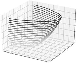
In the following we consider a cell indicated by  $C$ (central) and its neighbours indexed by an element from the set $N = \{E, W, T, B, F, R\}$, indicating the neighbour in the ‘east’, ‘west’, ‘top’, ‘bottom’, ‘front’ or ‘rear’ direction, see figure 1. The corresponding cell faces are identified by lower case letters from $s = \{e, w, t, b, f, r\}$, standing again for ‘east’, ‘west’, etc. According to this nomenclature, variables referring to the faces of the cell are indicated by subscript $e$,
$e$,  $w$, etc. and variables referring to the body of the neighbouring cells by subscript $E$,
$E$,  $W$, etc. With these definitions, the surface integral in (4.3) expands to
 \begin{equation} \frac{\partial \bar{U}_C}{\partial t} ={-} \frac{1}{\Delta x} \left( \bar{F}_{x,e}^c - \bar{F}_{x,w}^c \right) - \frac{1}{\Delta y} \left( \bar{F}_{y,t}^c - \bar{F}_{y,b}^c \right) - \frac{1}{\Delta z} \left( \bar{F}_{z,f}^c - \bar{F}_{z,r}^c \right), \end{equation}
where  $\bar {F}_{i,j}^c$ with $j\in s$ denoting the spatial average of the $i$th component of the convective flux over the cell face $j$, at time $t$. For the east cell face, we have, for instance,
 \begin{equation} \bar{F}_{x,e}^c = \frac{1}{\Delta y} \frac{1}{\Delta z} \int\limits_{y_{j-1/2}}^{y_{j+1/2}} \textrm{d} y \,\int\limits_{z_{k-1/2}}^{z_{k+1/2}} \,\mathrm{d} z \, F_{x,e}. \end{equation}
In the subsequent derivations we restrict ourselves to  $\bar {F}_{x,e}^c$, the remaining fluxes are treated analogously.

Figure 1. A finite volume cell in three dimensions with Cartesian topology. The neighbouring cells are indexed by capital letters  $E$ (east), $W$ (west), $T$ (top), $B$ (bottom), $F$ (front) and $R$ (rear). The corresponding cell faces are indicated by lower case letters.
We approximate the integrals in (4.5) by Gaussian quadrature with two sampling points in each direction as illustrated in figure 2
 \begin{equation} \bar{F}_{x,e}^c \approx \sum_{\alpha=1}^2 \sum_{\beta=1}^2 F_{x,e}^c (y_{\alpha}, z_{\beta}, t) \, \omega_{\alpha} \omega_{\beta}, \end{equation}
where the arguments  $y_{\alpha }$ and $z_{\beta }$ are the coordinates of the integration points on the east surface and $\omega _{\alpha }, \omega _{\beta }$ are the corresponding weights.

Figure 2. Illustration of the coordinates (filled circles) used for Gaussian quadrature with respect to the east cell face for the integration in (4.5).
Equation (4.6) involves the values  $F_{x,e}^c$ of the convective flux at the quadrature points, which, in turn, depend on the conservative field variables $U$ according to (2.5b). Indeed, we would need the values of $U$ at the quadrature points, however, according to our finite volume discretization, (4.4), only the cell averages of $U$ are available. Therefore, we interpolate the values of $U$ at the quadrature points from cell averages of $U$ of the cell where the quadrature points are located and the values of $U$ in a certain neighbourhood of this cell. This interpolation is delicate as it determines the shock capturing abilities of the numerical scheme.
Here we use a fifth-order weighted essentially non-oscillatory (WENO) scheme (Liu, Osher & Chan Reference Liu, Osher and Chan1994) that provides an acceptable balance of accuracy and efficiency and delivers fifth-order accuracy in smooth regions of the field and third-order accuracy near discontinuities. For the one-dimensional case, WENO is explained in detail by Liu et al. (Reference Liu, Osher and Chan1994). For the extension to three-dimensional problems we additionally apply the method of dimension-by-dimension interpolation by Titarev & Toro (Reference Titarev and Toro2004).
The quadrature points on the east face of a cell centred at  $x_i$ coincide with the quadrature points on the west face of the neighbouring cell centred at $x_{i+1}$. However, the interpolation of $U$ at the east face of a cell centred at $x_i$ ( $U_L\equiv U_e(x_i,y_\alpha ,z_\beta )$) is different from the interpolated value at the west face of the neighbouring cell at $x_{i+1}$ ( $U_R\equiv U_w(x_{i+1},y_\alpha ,z_\beta )$), because a different stencil is considered for each interpolation. This deviation leads to a violation of conservation laws because $U_L\neq U_R$ implies that the flux leaving the cell centred at $x_i$ at its east face differs from the flux that enters the neighbouring cell centred at $x_{i+1}$ at its west face. Therefore, the difference between $U_L$ and $U_R$ needs to be corrected. As shown e.g. in Toro (Reference Toro2013), the naïve approach of using the average of $U_L$ and $U_R$ leads to instabilities. Therefore, the flux between two neighbouring cells has to be derived from more elaborate upwind schemes that account for the direction of the flow. Moreover, to suppress spurious oscillations near discontinuities, the upwind scheme should assure monotonic flux. The multi-stage scheme by Titarev & Toro (Reference Titarev and Toro2004) fulfils both criteria. The key idea of this scheme is to predict the flux from the initial data $U_L, U_R$ and then to evolve $U_L$ and $U_R$ iteratively via the governing equation (3.1a,b). Here we use the first-order centred (FORCE) flux as a predictor
 \begin{equation} \left.\begin{gathered} U^{1/2} = \frac{1}{2} \left( U_L^{(l)} + U_R^{(l)} \right) - \frac{1}{2} \frac{\Delta t}{\Delta x} \left[ F \left(U_R^{(l)}\right) - F \left(U_L^{(l)}\right) \right] \\ F_{{FORCE}}^{(l)} = \frac{1}{4} \left\{ F \left(U_L^{(l)}\right) + F \left(U_R^{(l)}\right) + 2F \left(U^{1/2}\right) - \frac{\Delta t}{\Delta x} \left( U_R^{(l)} - U_L^{(l)} \right) \right\}, \end{gathered}\right\} \end{equation}
where  $U_R^{(l)}$ and $U_L^{(l)}$ denote the $l$th iterations of the vector of conservative variables
 \begin{gather} U_L^{(l+1)} = U_L^{(l)} - \frac{\Delta t}{\Delta x} \left[ F_{{FORCE}}^{(l)} - F \left(U_L^{(l)}\right) \right], \end{gather}
 \begin{gather}U_R^{(l+1)} = U_R^{(l)} - \frac{\Delta t}{\Delta x} \left[ F \left(U_R^{(l)}\right) - F_{{FORCE}}^{(l)} \right]. \end{gather}
We terminate the above iteration after  $k$ steps once the relative error of the predictor flux $F_{{FORCE}}$ is less than one per cent and assume $F=F_{{FORCE}}^{(k)}$.
We can now compute the right-hand side of (4.4). The numerical solution of the convective equation (3.1a,b) corresponds to the solution of the ordinary differential equation (4.4). For this purpose we apply the third-order total variation diminishing Runge–Kutta method derived by Gottlieb & Shu (Reference Gottlieb and Shu1998). The corresponding time iteration reads
 \begin{equation} \left.\begin{gathered}
U^{(1)} = U (t) + \Delta t \mathcal{L} \left(U (t)\right)
\\ U^{(2)} = \tfrac{3}{4}U (t) + \tfrac{1}{4} U^{(1)} +
\tfrac{1}{4} \Delta t \mathcal{L}\left(U^{(1)}\right) \\ U
(t+\Delta t) = \tfrac{1}{3}U (t) + \tfrac{2}{3} U^{(2)} +
\tfrac{2}{3} \Delta t \mathcal{L}\left(U^{(2)}\right)
\end{gathered}\right\}
\end{equation}
\begin{equation} \left.\begin{gathered}
U^{(1)} = U (t) + \Delta t \mathcal{L} \left(U (t)\right)
\\ U^{(2)} = \tfrac{3}{4}U (t) + \tfrac{1}{4} U^{(1)} +
\tfrac{1}{4} \Delta t \mathcal{L}\left(U^{(1)}\right) \\ U
(t+\Delta t) = \tfrac{1}{3}U (t) + \tfrac{2}{3} U^{(2)} +
\tfrac{2}{3} \Delta t \mathcal{L}\left(U^{(2)}\right)
\end{gathered}\right\}
\end{equation}
where the operator  $\mathcal {L}$ corresponds to the right-hand side of (4.4).
5. Solution operator of the diffusion equation
We rewrite the diffusive flux  $F_i^{\nu } (U, \boldsymbol {\nabla } U)$ in (3.1a,b) by means of diffusion matrices $D_{ij}$ $(i,j\in \{x,y,z\})$,
 \begin{equation} F_i^{\nu} (U, \boldsymbol{\nabla} U) = D_{ix} \partial_x U + D_{iy} \partial_y U + D_{iz} \partial_z U, \end{equation}
where  $\partial _x U = (\partial _x U_1, \partial _x U_2, \partial _x U_3, \partial _x U_4, \partial _x U_5)^\textrm {T}$ and analogously for $\partial _y U$ and $\partial _z U$. The diffusion matrices $D_{ij}$ are derived in Appendix A. These matrices are not restricted to the structured meshes used in this work, they can also be applied for e.g. triangular or tetrahedral meshes. We define further $\boldsymbol {\nabla } U\equiv (\partial _x U, \partial _y U, \partial _z U)^\textrm {T}$ and
 \begin{equation} \mathbb{D} = \begin{pmatrix} D_{xx} & D_{xy} & D_{xz} \\ D_{yx} & D_{yy} & D_{yz} \\ D_{zx} & D_{zy} & D_{zz} \end{pmatrix}, \end{equation}
to write the diffusive flux in the form
 \begin{equation} \boldsymbol{F}^{\nu} (U, \boldsymbol{\nabla} U) = \mathbb{D} (U) \boldsymbol{\cdot} \boldsymbol{\nabla} U = D_{ij} \partial_i U\,. \end{equation}
Equation (3.2a,b) can then be written as
 \begin{equation} \partial _t U = \boldsymbol{\nabla} \boldsymbol{\cdot} \left[ \mathbb{D} \boldsymbol{\cdot} \boldsymbol{\nabla} U \right] + S(U). \end{equation}
Similar as for the convection equation, we map this partial differential equation to a set of algebraic equations by means of the finite volume approach. The finite volume integration of (5.4) reads
 \begin{equation} \mathop{\int}\limits_{\Delta V} \,\mathrm{d} V \, \partial _t U = \int\limits_{\Delta S} \mathrm{d} S \, \boldsymbol{n} \boldsymbol{\cdot} \left[\mathbb{D} \boldsymbol{\cdot} \boldsymbol{\nabla} U \right] + \mathop{\int}\limits_{\Delta V} \,\mathrm{d} V \, S(U), \end{equation}
where we again used the divergence theorem, to replace the first integral on the right-hand side over the volume element  $\Delta V$ by an integral over its surface $\Delta S$.
The diffusion matrices can be split into diagonal and non-diagonal (cross-diffusion) contributions. For the case of a Cartesian mesh, Darwish & Moukalled (Reference Darwish and Moukalled2009) have shown that only the diagonal terms,  $D_{ii}$, contribute to the solution. In this case, the surface integral over the diffusive fluxes can be written as
 \begin{equation} \int\limits_{\Delta S} \mathrm{d} S \, \boldsymbol{n} \boldsymbol{\cdot} \left(\mathbb{D} \boldsymbol{\cdot} \boldsymbol{\nabla} U \right) = \sum_{i \in \{x,y,z\}} \left(D_{ii} \partial_i U \right) \Delta S_{i}, \end{equation}
where  $\Delta S_{i}$ is the surface element with the normal pointing in the $i$-direction, e.g. $\Delta S_{x} = \Delta y \Delta z$.
If we expand the sum on the right-hand side over all faces and use a central difference approximation for the derivatives, the diffusive equation reads
 \begin{align} \frac{\mathrm{d} U_C}{\mathrm{d} t} &= D_{xx} (U_{e}) \frac{U_{E}-U_C}{\Delta x^2} - D_{xx} (U_{w}) \frac{U_C-U_{W}}{\Delta x^2} + D_{yy} (U_{t}) \frac{U_{T}-U_C}{\Delta y^2} \nonumber\\ &\quad- D_{yy} (U_{b}) \frac{U_C-U_{B}}{\Delta y^2} + D_{zz} (U_{f}) \frac{U_{F}-U_C}{\Delta z^2} - D_{zz} (U_{r}) \frac{U_C-U_{R}}{\Delta z^2} + S(U_C). \end{align}
For convenience, we define
 \begin{equation} \left.\begin{gathered} a_{E} = \frac{D_{xx} (U_{e})}{\Delta x^2}, \quad a_{W} = \frac{D_{xx} (U_{w})}{\Delta x^2}, \quad a_{T} = \frac{D_{yy} (U_{t})}{\Delta y^2}, \\ a_{B} = \frac{D_{yy} (U_{b})}{\Delta y^2}, \quad a_{F} = \frac{D_{zz} (U_{f})}{\Delta z^2}, \quad a_{R} = \frac{D_{zz} (U_{r})}{\Delta z^2}, \\ a_{C} ={-}(a_{E} + a_{W} + a_{T} + a_{B} + a_{F} + a_{R}), \end{gathered}\right\} \end{equation}
and rewrite (5.7) in compact form
 \begin{equation} \frac{\mathrm{d} U_C}{\mathrm{d} t} = a_{C}\, U_{C} + a_{E}\, U_{E} + a_{W}\, U_{W} + a_{T}\, U_{T} + a_{B}\, U_{B} + a_{F}\, U_{F} + a_{R}\, U_{R} + S(U_{C}). \end{equation}
 The ordinary differential equation (ODE) in (5.9) is stiff in regions of high packing fractions, where the kinetic coefficients such as, e.g. the viscosity diverge. This is particularly relevant for driven systems where granulates frequently change in the course of time between very rarefied and random close packing states. The application of explicit methods is problematic for stiff ODEs as an impractically small time step may be required to keep the numerical error bound. Explicit methods would, thus, significantly restrict the range of applicability of the numerical scheme. Therefore, we use an implicit Runge–Kutta method (Butcher Reference Butcher1964) to solve (5.9) for all grid cells. In general, a  $s$-stage Runge–Kutta scheme for the numerical solution of an initial value problem
 \begin{equation} \frac{\mathrm{d}\boldsymbol{U}}{\mathrm{d}t} = \boldsymbol{f}\left(\boldsymbol{U}\right),\quad \boldsymbol{U}\left(t_0\right)=\boldsymbol{U}_0, \end{equation}
reads
 \begin{equation} \boldsymbol{U}(t_0+\Delta t) \approx \boldsymbol{U}_0 + \Delta t \sum_{i=1}^{s} b_i \boldsymbol{f}\left(\boldsymbol{k}_i\right) \end{equation}
where
 \begin{equation} \boldsymbol{k}_i = \boldsymbol{U}_0 + \Delta t \sum_{j=1}^{s} a_{ij}\, \boldsymbol{f}\left(\boldsymbol{k}_j\right), \quad i=1, 2, \ldots, s \end{equation}
denotes the sampling points where the right-hand side of the ODE (5.10a,b) is evaluated. In general, (5.12) is a nonlinear system of equations which must be solved numerically to obtain the sampling points  $\boldsymbol {k}_i$. To this end, we use the modified Newton iteration scheme by Houbak, Nøsett & Thomsen (Reference Houbak, Nøsett and Thomsen1985). A scheme due to (5.12) can be specified by the coefficients $a_{ij}$ and $b_{i}$ which can be represented in a Butcher (Reference Butcher1964) table
 \begin{equation} \begin{array}{c|cccc} &
a_{11} & a_{12} & \cdots & a_{1s} \\ & a_{21} & a_{22} &
\cdots & a_{2s} \\ & \vdots & \vdots & & \vdots \\ & a_{s1}
& a_{s2} & \cdots & a_{ss} \\ \hline\\
& b_{1} & b_{2} & \cdots &
b_{s} \end{array} \end{equation}
\begin{equation} \begin{array}{c|cccc} &
a_{11} & a_{12} & \cdots & a_{1s} \\ & a_{21} & a_{22} &
\cdots & a_{2s} \\ & \vdots & \vdots & & \vdots \\ & a_{s1}
& a_{s2} & \cdots & a_{ss} \\ \hline\\
& b_{1} & b_{2} & \cdots &
b_{s} \end{array} \end{equation}
We implemented a two stage Gauss–Legendre quadrature formula which provides fourth-order accuracy. The coefficients of this scheme read
 \begin{equation} \begin{array}{c|cc} &
\dfrac{1}{4} & \dfrac{1}{4}-\dfrac{\sqrt{3}}{6}\\
&
\dfrac{1}{4}+\dfrac{\sqrt{3}}{6} & \dfrac{1}{4_{\vphantom{A_A}}}\\\hline\\
&
\dfrac{1^{\vphantom{A_A}}}{2} & \dfrac{1}{2} \end{array}
\end{equation}
\begin{equation} \begin{array}{c|cc} &
\dfrac{1}{4} & \dfrac{1}{4}-\dfrac{\sqrt{3}}{6}\\
&
\dfrac{1}{4}+\dfrac{\sqrt{3}}{6} & \dfrac{1}{4_{\vphantom{A_A}}}\\\hline\\
&
\dfrac{1^{\vphantom{A_A}}}{2} & \dfrac{1}{2} \end{array}
\end{equation}
The efficiency of the algorithm can be improved significantly by switching between this highly accurate scheme and a less accurate but more efficient scheme in regions where (5.9) does not reveal stiff behaviour. Such a switching between a highly accurate but numerically expensive algorithm and a numerically inexpensive implicit midpoint rule was proposed by Nørsett & Thomsen (Reference Nørsett and Thomsen1986). The implicit midpoint rule delivers second-order accuracy and its coefficients read in Butcher notation
 \begin{equation} \begin{array}{c|c} &
\dfrac{1}{2_{\vphantom{A_A}}}\\\hline\\ & \dfrac{1^{\vphantom{A_A}}}{2}
\end{array} \end{equation}
\begin{equation} \begin{array}{c|c} &
\dfrac{1}{2_{\vphantom{A_A}}}\\\hline\\ & \dfrac{1^{\vphantom{A_A}}}{2}
\end{array} \end{equation}
6. Boundary conditions
Three types of boundary conditions are especially relevant for granular systems: periodic boundaries, solid walls and oscillating walls. While the implementation of periodic boundaries is straightforward, there are different ways to model solid boundaries. First, one can extend the simulation domain by ghost cells. The hydrodynamic variables of these ghost cells are determined from the corresponding values of their neighbouring cells within the physical simulation domain whilst taking into account the mirror symmetry with respect to the bounding wall (Carrillo et al. Reference Carrillo, Pöschel and Salueña2008). For instance, to model a slip boundary condition with no mass flux through the wall, the normal component of the velocity field is inverted while the tangential component of the velocity field, as well as the energy field and the density field, are copied. Similarly, a no-slip boundary can be achieved by additionally inverting the tangential component of the velocity field.
Another way to model boundary conditions is to determine the hydrodynamic variables on the boundary explicitly (Blazek Reference Blazek2015). This approach reduces the numerical errors due to the interpolation of the fluxes on the boundary surface. It is, thus, more consistent with the applied finite volume method. To represent slip boundaries, only the normal component of the velocity field is set to zero at the boundary, while for a no-slip boundary all components of the velocity field are set to zero at the boundary. For the no-slip solid wall the convective and diffusive fluxes in (2.5b) and (2.5c), reduce to
 \begin{equation} F_{i}^c (U)= \begin{bmatrix} 0 \\ \delta_{xi} \dfrac{p_w}{m} \\ \delta_{yi} \dfrac{p_w}{m} \\ \delta_{zi} \dfrac{p_w}{m} \\ 0 \end{bmatrix}\quad\text{and}\quad F_{i}^{\nu} (U, \boldsymbol{\nabla} U) = \begin{pmatrix} 0 \\ 0 \\ 0 \\ 0 \\ - q_i \end{pmatrix}, \end{equation}
where  $p_w$ denotes the pressure at the wall which can be extrapolated from the neighbouring cells within the simulation domain (Blazek Reference Blazek2015) and $q_i$ is the heat flux through the boundary. In case of elastic walls, there is no energy loss and the heat flux $q_{i}$ vanishes at the boundary. If the interaction between the boundary and the particles of the granulate is dissipative, there is a finite heat flux through the boundary. This heat flux is determined by the mean collision frequency, $\nu _0$, at which the particles collide with the boundary (Brilliantov & Pöschel Reference Brilliantov and Pöschel2010) and by the coefficient of restitution $\varepsilon _w$ which describes the fraction of energy that is dissipated when a grain collides with the wall
 \begin{equation} q_i= \frac{1}{2} m u_i \nu_0 \frac{1-\varepsilon_w^2}{A_s}, \end{equation}
where  $A_s$ denotes the surface area of the boundary. Equation (6.2) is obtained by multiplying the mean energy loss of a particle impacting the wall by the mean collision frequency per surface area.
In many cases, granular systems are driven by mechanically vibrating walls with a certain frequency and amplitude. The corresponding oscillating walls can be modelled by rewriting the hydrodynamic equations (2.4) in the non-inertial frame of the vibrating walls (Carrillo et al. Reference Carrillo, Pöschel and Salueña2008). The corresponding inertial forces act on all particles in the system, irrespective of their position. Therefore, in case of driven systems, inertial forces have to be added to the momentum equation in (2.4).
The interaction between granular matter and the system boundaries can be much more complicated. The grains can, e.g. roll along the boundary surface. Additionally, the shape and the surface roughness of the grains have great impact on the boundary–bulk interaction. However, these grain-level details are not subject of a hydrodynamic model.
7. Numerical validation
Because of the complexity of the hydrodynamic equations, (2.4), a theoretical validation of the presented numerical scheme is not feasible. To our knowledge, there are no experimental results, in which temperature, velocity and density are measured simultaneously, which precludes us from an experimental validation of our approach as well. Therefore, we validate our hydrodynamic simulations against well-established particle-based simulations of the corresponding granular system. For the validation we consider the following scenarios:
(i) a granular gas which sediments under the action of gravity;
(ii) a bed of grains in a vertically shaken container in presence of gravity; and
(iii) the flow of granular material down an inclined pile.
These set-ups are demanding, regarding a hydrodynamic simulation because they involve extreme variations of the packing fraction, from dilute gas to random close packing, and steep gradients in the hydrodynamic fields. For the particle-based reference simulations we apply event driven molecular dynamics (EDMD) and the discrete element method (DEM) (see, e.g. Pöschel & Schwager (Reference Pöschel and Schwager2005), and many references therein). Both methods describe the granular systems reliably on different levels of detail.
7.1. Sedimentation test
First, we consider the sedimentation of a homogeneous gas of 190 985 spherical particles under the action of gravity. The particles are enclosed by a rectangular box of size  $0.1\times 0.1\times 0.1\ \mathrm {m}^3$. The walls of this box are modelled by solid elastic planes on the top and floor and by periodic boundaries in the horizontal directions. The particles are of diameter $1\ \mathrm {mm}$ and of material mass density $2600\ \mathrm {kg}\ \mathrm {m}^{-3}$. For the hydrodynamic simulations, the domain is divided into $50 \times 100 \times 50$ Cartesian grid cells and the time step $10^{-6}\ \mathrm {s}$ is used.
An EDMD simulation is considered as the reference for this test. In EDMD simulations, the particles are modelled ideally rigid. A collision between two ideally rigid, smooth particles corresponds to an instantaneous transfer of momentum, that is, to an instantaneous change of the particles’ velocities. Collisions are characterized by the coefficient of restitution,  $\varepsilon$ relating the pre- and post-collisional values of the normal components of the particles’ relative velocities at the point of contact. In our simulation we assume $\varepsilon = 0.9$. Further details on event-driven molecular dynamics can be found e.g. in Bannerman, Sargant & Lue (Reference Bannerman, Sargant and Lue2011) and references therein.
To compare the results of the hydrodynamic simulations with the results of the particle-based EDMD simulations, continuous hydrodynamic fields, such as density, flow velocity and energy density, have been computed from the discrete particle data. For the sedimentation test, the system is homogeneous in the horizontal direction while gravity acts in the vertical direction, therefore, we can represent the fields as functions of the vertical component (height). Figure 3 compares the conservative variables (density, momentum density and energy density) as functions of the height (direction of gravity) as obtained from the hydrodynamic simulations with those obtained from the reference EDMD simulations. We see that the field of density is well described by the hydrodynamic approach for all times and heights. For the fields of velocity and energy, the hydrodynamic description and the particle-based reference simulation are in good agreement for times up to approximately 100 ms. For later times, we still see qualitative agreement of the curves, however, the values deviate moderately. Similar behaviour can be observed for the field of temperature shown in figure 4. The numerical results are not affected by substantial refinements of the spatial and temporal resolutions of the numerical scheme which indicates the reliability of our numerical solution. We therefore attribute the deviations to deficiencies of the underlying continuum mechanical model. The constitutive relations provided by Garzó & Dufty (Reference Garzó and Dufty1999) and the applied equation of state are approximations to the physics of granulates. As the applied constitutive relations are derived from kinetic theory, they are only valid for dynamic systems. The deviations start to get significant when part of the grains rest on the floor ( $t=150\ \text {ms}$). Additionally, the hydrodynamic equations we solve are approximated to first-order derivatives which may cause error when sharp gradients in the hydrodynamic fields are present. To improve the accuracy, one should apply hydrodynamic equations beyond the Navier–Stokes level and incorporate terms of Burnett order and super-Burnett order (Chapman & Cowling Reference Chapman and Cowling1939; Sela, Goldhirsch & Noskowicz Reference Sela, Goldhirsch and Noskowicz1996; Sela & Goldhirsch Reference Sela and Goldhirsch1998; Goldhirsch Reference Goldhirsch1999, Reference Goldhirsch2001; Jin & Slemrod Reference Jin and Slemrod2001; Goldhirsch Reference Goldhirsch2008; Gupta Reference Gupta2012; Saha & Alam Reference Saha and Alam2020). Despite the fully three-dimensional simulations which have been applied, the present sedimentation test is effectively a one-dimensional problem. However, to our knowledge, it is the first test case in which all relevant variables (density, momentum and energy) as obtained from a hydrodynamic simulation are compared with the corresponding results from the particle system.

Figure 3. Comparison of the conservative variables as functions of the height as obtained from the hydrodynamic simulations (black line) and those obtained from the reference EDMD simulation (red circles). The top row shows the density field, the middle row shows the vertical velocity times density and the bottom row shows the energy density. Each column from left to right corresponds to an instant of time  $t=50\ \text {ms}$, $t=100\ \text {ms}$, $t=150\ \text {ms}$, respectively.

Figure 4. Comparison of the temperature field as a function of the height as obtained from the hydrodynamic simulations (black line) and from the reference EDMD simulation (red circles), for different values of time ( $t=50\ \text {ms}$, $t=100\ \text {ms}$, $t=150\ \text {ms}$). Different from figure 3, the range of the abscissas is reduced $0.04\ \text {m}$ as all features of interest are contained in this smaller interval.
7.2. Bouncing bed test
We consider granular particles under the action of gravity in a vertically shaken container. This system exhibits various modes of behaviour. In an elaborate experimental study, this rich behaviour was compiled to a phase diagram by Eshuis et al. (Reference Eshuis, van der Weele, van der Meer, Bos and Lohse2007). For a quantitative evaluation of our hydrodynamic simulations, we compare the hydrodynamical results with those obtained from corresponding particle-based discrete element simulations, that is, we solve Newton's equation of motion for the translational and rotational motion of all  $N$ grains.
When particles collide, they mutually deform each other, quantified by
 \begin{equation} \xi = \max \left( 0,R_i+R_j-r_{ij} \right), \end{equation}
where  $R_i$ and $R_j$ are the radii of the particles and $r_{ij}=|\boldsymbol {r}_{ij}|$ is the absolute value of the inter-centre relative vector $\boldsymbol {r}_{ij}=\boldsymbol {r}_j-\boldsymbol {r}_i$. The deformation causes a repulsive interaction force $\boldsymbol {f}$ which can be decomposed into a normal component $\boldsymbol {f}_n$ in direction of $\boldsymbol {e}_n = \boldsymbol {r}_{ij}/|\boldsymbol {r}_{ij}|$ and a tangential component $\boldsymbol {f}_t$ perpendicular to $\boldsymbol {e}_n$
 \begin{gather} \boldsymbol{f}=\boldsymbol{f_n}+\boldsymbol{f_t} \end{gather}
 \begin{gather}\boldsymbol{f}_{\boldsymbol{n}}=(\boldsymbol{f}\boldsymbol{\cdot}\boldsymbol{e}_n) \boldsymbol{e}_n\equiv f_n\boldsymbol{e}_n \end{gather}
 \begin{gather}\boldsymbol{f}_{\boldsymbol{t}}=\boldsymbol{f}-\boldsymbol{f}_n\equiv f_t \boldsymbol{e}_t. \end{gather}
For viscoelastic particles, the normal component reads (Brilliantov et al. Reference Brilliantov, Spahn, Hertzsch and Pöschel1996)
 \begin{equation} f_{n}= \rho_{{el}} \xi^{3/2}-\frac{3}{2}A_{{dis}}\rho_{{el}} \dot{\xi}\sqrt{\xi}, \end{equation}
where
 \begin{equation} \rho_{{el}}= \frac{2Y\sqrt{R_{{eff}}}}{3(1-\nu^{2})}, \end{equation}
where  $Y$ and $\nu$ denote Young's modulus and Poisson's ratio, respectively, and $R_{{eff}}=R_iR_j/(R_i+R_j)$. The dissipative parameter $A_{{dis}}$ is a function of the material viscosity, see
Brilliantov et al. (Reference Brilliantov, Spahn, Hertzsch and Pöschel1996). As the coefficient of restitution is a (known) function of the interaction force (Schwager & Pöschel Reference Schwager and Pöschel1998a,Reference Schwager and Pöschelb; Ramírez et al. Reference Ramírez, Pöschel, Brilliantov and Schwager1999) and the interaction velocity, the coefficient  $A_{{dis}}$ can be determined provided the coefficient of restitution for a particular collision rate is known (Müller & Pöschel Reference Müller and Pöschel2011), for instance from an experiment.
The tangential component of the interaction force causes a torque on the colliding particles, which, in turn, alters their angular velocity. Here, we apply the model by Cundall & Strack (Reference Cundall and Strack1979) which mimics static and dynamic friction by means of an imaginary spring (for an extended discussion see Pöschel & Schwager Reference Pöschel and Schwager2005; Schwager, Becker & Pöschel Reference Schwager, Becker and Pöschel2008). The spring of initial length zero is created at time  $t_c$ when the particles touch. Its elongation is then
 \begin{equation} Z (t) =\int_{tc}^{t}v_{{rel}}^t(t^{\prime})\,\textrm{d}t^{\prime}, \end{equation}
where  $v_{rel}^t\equiv \boldsymbol {e}_t\boldsymbol {\cdot }[\dot {\boldsymbol {r}}_{ij}+\boldsymbol {e}_n\times (R_i\boldsymbol {\omega }_i+R_j\boldsymbol {\omega }_j)]$ is the tangential component of the relative velocity of the particles at the point of contact and $\boldsymbol {\omega }_i$ and $\boldsymbol {\omega }_j$ are the angular velocities of particles $i$ and $j$. The tangential component of the interaction force is then given by the restoring force of the spring, limited by Coulomb's law
 \begin{equation} f_{t}={-}\operatorname{sign}(v_{{rel}}^t)\cdot \min(\left | KZ\right | ,\mu |\,f_n|). \end{equation}
Here,  $\mu$ denotes Coulomb's coefficient of friction and $K$ is the elastic constant of the spring. In contrast to the normal force, the parameters of the tangential force, $K$ and $\mu$, cannot be determined from material bulk properties and geometry but they are mainly determined by surface properties. In practice, they can be only determined by comparison of the results of benchmark simulations and experimental results. For the bouncing bed test, we consider a rectangular box with of size $L_x\times L_y\times L_z=100\times 100\times 10 \ \mathrm {mm}^3$, filled by 8560 particles of diameter 1 mm. The material parameters used in the simulation read $Y=5\times 10^9\ \text {Pa}$, material density $2.6\ \text {g}\ \text {cm}^{-3}$, $\nu =0.3$, $A_{{dis}}=1.61\times 10^{-7}\ \textrm {s}$, $K=0.347 \rho _{{el}}\sqrt {R_{eff}}$ and $\mu =0.7$. The particles are vertically vibrated in the presence of gravity with the frequency $12 \ \mathrm {Hz}$ and the amplitude $4 \ \mathrm {mm}$. For the interaction between particles and the wall we assume the same parameters. The integration time step is $10^{-5}$ s.
To compare the results of the DEM simulation with the results of the corresponding hydrodynamic simulations, the domain is divided into  $20 \times 100 \times 4$ Cartesian grid and a time step of ${1}/{12}\times 10^{-5}\ \mathrm {s}$ is used. We consider the time-dependent density field as a function of the vertical coordinate, again averaged over the homogeneous horizontal dimensions. We assume no-flux boundary conditions at the upper side of the simulation domain near the free surface. Figure 5 shows the packing fraction as a function of the distance from the bottom wall as obtained from the hydrodynamic simulations in comparison with the results from the corresponding DEM simulation. The results of both methods are in good quantitative agreement for all phases of the vibration cycle. Similar results were obtained before by e.g. Bougie, Policht & Pearce (Reference Bougie, Policht and Pearce2012). There, however, mild driving conditions are considered which lead to maximum volume fractions way below 0.3. In our study we apply driving parameters causing packing fractions larger than 0.5. Due to the extreme conditions of the bouncing bed set-up (dynamic transitions between densely packed and dilute regions) the temperature cannot be reliably obtained from particle simulations. For high density where the granulate occurs in an almost crystalline or random close packed state, the relative velocities of the grains obtained from particle simulations are dominated by unavoidable numerical noise, which impedes a meaningful evaluation of the granular temperature. For the dilute extreme, the number of particles in these regions is almost zero; see, e.g. figure 5(b) for small height. Thus, in extremely dilute regions, we cannot compute the value of granular temperature from particle simulation data. Nevertheless, the temperature as obtained from granular hydrodynamics can be computed also in the dilute and the densely packed regions, and this is shown in the bottom raw of figure 5.

Figure 5. (a–c) Snapshots from the hydrodynamic- and particle-based simulations. Each of the panels is subdivided into an upper part showing the density field obtained from the hydrodynamic simulations, while the lower part shows a snapshot of the DEM simulation. (d–f) Field of packing fraction (density) as a function of distance from bottom wall, as obtained from hydrodynamic simulations (red lines) in comparison with results from DEM simulations (blue circles). (g–i) Granular temperature obtained from hydrodynamic simulations. Each column corresponds to a certain phase of the oscillation cycle,  $0.3\ T$ (a,d,g), $0.6\ T$ (b,e,h) and $0.9\ T$ (c,f,i), where $T$ is the period of vibration. The coefficient of restitution was $\varepsilon =0.9$.
7.3. Flow on a pile with rough sidewalls
The development of general constitutive relations for the continuum description of granular flows is still work in progress. The constitutive relations for the gas regime can be derived from kinetic theory (see, e.g. Goldhirsch Reference Goldhirsch2003) and for the solid regime from soil mechanics (see, e.g. Nedderman Reference Nedderman1992). A constitutive law for dense granular flow is proposed by Jop et al. (Reference Jop, Forterre and Pouliquen2006), where the granular flow is described as incompressible with a simple visco-plastic relation for viscosity. The law of Jop et al. (Reference Jop, Forterre and Pouliquen2006) is rate independent to the extent that only the coefficient of friction depends on the shear rate. While the constitutive law by Jop et al. (Reference Jop, Forterre and Pouliquen2006) leads to excellent agreement with experiments, it provides no information about packing fraction and velocity fluctuations inside the bulk.
In this section, we consider glass beads of diameter  $\sigma = 1\ \mathrm {mm}$, in a channel of length $226\ \mathrm {cm}$ and width $w=48 \sigma$, with rough sidewalls. The thickness of the flowing material, $h$, is initialized to 22.5 mm. The channel is tilted by angle $\theta = 27 ^{\circ }$. Figure 6 shows a sketch of the set-up. To compare our results with the simulations by Silbert et al. (Reference Silbert, Landry and Grest2003) and Jop et al. (Reference Jop, Forterre and Pouliquen2006), we define the dimensionless flow rate $Q^{\star }=Q/(\sigma ^{3/2} g^{1/2})$, where $Q$ is the flow rate per unit of width $w$,
$w$,  $g$ is the gravitational acceleration and $V^{\star }=V/(g\sigma )^{1/2}$ is the dimensionless velocity in the $x$ direction.

Figure 6. Schematic view of the granular material (dark grey) flowing down a pile between rough sidewalls. The pile is tilted by the angle  $\theta$ with respect to the horizon. Therefore, the material is driven by gravity resulting in a flow in the $x$-direction.
The model by Jop et al. (Reference Jop, Forterre and Pouliquen2006) describes dense granular flow as an incompressible fluid (see discussion in § 2). Here, we solve the full Navier–Stokes equations (2.4) using the constitutive relations from Garzó & Dufty (Reference Garzó and Dufty1999). We discretize the domain into a  $80 \times 80 \times 40$ structured grid and use the time step $10^{-6}\ \mathrm {s}$ for the time integration. The rough sidewalls and the channel floor are considered as no-slip boundaries, as described in § 6. We assume no-flux boundary conditions at the upper side of the simulation domain near the free surface.
The first consequence of solving the full equations (2.4) is that the volume fraction is no longer constant. Figure 7 shows the profile of the packing fraction along the  $y$ direction. As expected, in the lower part of the flow, the material is more dense, while there is a dilute gaseous region on the surface of the pile. The existence of this gaseous region is in good agreement with the experiment performed by Forterre & Pouliquen (see, e.g. figure 1 in Forterre & Pouliquen Reference Forterre and Pouliquen2008). For a more quantitative comparison, figure 7 shows experimental results by Ancey (Reference Ancey2001) for channel flow of glass beads of 1 mm diameter down a rough incline (width 48 mm, slope $27^{\circ }$, layer thickness 26 mm), see figure 17 in Ancey (Reference Ancey2001). We find good agreement between the experimental and numerical density profiles. The different asymptotic density ( $\varPhi$ for small $y$) may be attributed to the fact that the experiment uses slightly polydisperse grains (‘poorly sorted’, no interval given, see table 1 in Ancey Reference Ancey2001). Note that the width of the numerically obtained profile in figure 7 extends to $y\approx 26\ \text {mm}$, which is larger than the initial layer width, $h$, given above. This inflation can be explained by Reynolds dilatancy of the flowing sand. The initial height, $h$, has been chosen such that the width of the stationary flow reaches approximately the same extension as the experimental data.

Figure 7. Profile of the packing fraction, perpendicular to the direction of the flow (solid line). The coefficient of restitution was  $\varepsilon =0.9$. The vertical axis is chosen such that $y/\sigma =0$ is the height of a fixed plane near the surface of fluctuating height. For comparison with the experiment, the symbols and dashed line show the density profile measured for channel flow of glass beads of 1 mm diameter down a rough incline (width 48 mm, slope $27^{\circ }$, layer thickness 26 mm), see figure 17 in Ancey (Reference Ancey2001). We find good agreement between the experimental and numerical density profiles. The different asymptotic densities ( $\varPhi$ for small $y$) may be attributed to the fact that the experiment uses slightly polydisperse grains, whose density at random close packing is larger than for monodisperse spheres.)
The three-dimensional velocity profile resulting from the hydrodynamic simulation is shown in figure 8. Due to the rough sidewalls and the rough base of the pile, the velocity is lower close to these surfaces. In our simulation, the velocity profile decays slower as compared to the simulations by Jop et al. (Reference Jop, Forterre and Pouliquen2006). The reason, therefore, is that the viscosity is independent of pressure and only depends on temperature and filling fraction in our constitutive relations. On the contrary, the viscosity depends on pressure in the constitutive relations by Jop et al. (Reference Jop, Forterre and Pouliquen2006). As the pressure is higher at the bottom of the channel, the viscosity diverges to infinity faster. As a result, lower velocities are observed close to the bottom of the channel in Jop et al. (Reference Jop, Forterre and Pouliquen2006).

Figure 8. The three-dimensional velocity profile for a granulate flowing down an inclined pile between two rough sidewalls shows that the maximum velocity is attained on the top surface of the granulate and on the centreline between the two sidewalls. The vertical axis is chosen such that  $y/\sigma =0$ is the height of a fixed plane near the surface of fluctuating height. Thus, at $y/\sigma \approx -50$, the flow velocity almost ceases. The coefficient of restitution was $\varepsilon =0.9$.
8. Summary
We presented a numerical scheme for the hydrodynamic simulation of granular systems in three dimensions. To our knowledge, this is the first general three-dimensional simulation algorithm for granular hydrodynamics which is neither restricted to certain dynamic states of the granulate nor to special boundary conditions. Most importantly, unlike previous methods used, e.g. in soil mechanics or rapid gas flows, our method is not restricted to a certain range of density. While, by construction, our numerical method covers grain-inertia flows, it was demonstrated that the algorithm is numerically robust for all values of packing fraction, from dilute gas to random close packing and likewise also with respect to harsh driving. However, one has to distinguish between the above-mentioned capabilities of the numerical scheme used to solve the Navier–Stokes equations, on the one hand, and the validity of the applied constitutive relations, on the other. The fundamental prerequisites to successfully apply the presented algorithm are, of course, constitutive relations which are valid over the whole range of densities and flow regimes. While massive advances have been made in this direction over the past twenty years, this ultimate research objective is still unreached.
Comparison of the presented numerical scheme against well-established particle-based simulation techniques reveals two important points:
(i) There are situations where the hydrodynamic results are in very good qualitative and quantitative agreement with the particle-based reference simulations. In these cases, both simulation methods support one another and we can assume that both methods are correct, including the underlying hydrodynamic model and the numerical scheme presented here.
(ii) There are situations where we find qualitative agreement between the hydrodynamic and particle simulations, however, non-negligible quantitative deviations between the numerical data gained by hydrodynamics and particle mechanics. This, in turn, may be due to three different arguments:
(a) The underlying hydrodynamic model is inadequate, that is, either the constitutive equations or the equation of state are inappropriate for the investigated system. This is not surprising as all available constitutive relations and equations of state are approximative and based on phenomenological arguments rather than on rigorous derivations.
(b) Particularly for systems at large packing density, the Navier–Stokes level of the hydrodynamic description may be insufficient, that is, linear relations for the transport coefficients may be insufficient for the description of granular flow at high density. In this case, higher-order descriptions on Burnett or super-Burnett order must be considered, see the discussion in § 7.1.
(c) The hydrodynamic description itself may be inadequate due to the arguments related to the lack of scale separation discussed at the end of § 1. In these cases, there is no hope for a hydrodynamic description. Fortunately, sufficiently dynamic systems of practical interest seem not to belong to this class. Our demonstration examples have been chosen to be hard for a hydrodynamic description, but still we could obtain stable results in approximate quantitative agreement with particle simulations.
It would be desirable to compare our results with competing approaches to solve the equations (2.4). However, all available studies apply explicit schemes and fail in the dense regime. A comparison which is restricted to the dilute limit is, however, inappropriate as the aim of the presented implicit method is neither to increase performance nor to optimize accuracy but only to improve the stability of the solver and, finally, to enable simulations in the dense regime.
The computational granular hydrodynamics presented here can be extended and generalized to other constitutive relations (e.g. Jenkins & Richman Reference Jenkins and Richman1986), and equations of state (e.g. Luding Reference Luding2009), available in the literature. The reliable and numerically stable hydrodynamic simulation method finally allows us to study large-scale granular systems which are not accessible through particle simulations due to the large number of particles involved, such as sand dunes (e.g. Schwämmle & Herrmann Reference Schwämmle and Herrmann2003), planetary rings (e.g. Grenberg & Brahic Reference Grenberg and Brahic1984; Esposito Reference Esposito2006; Fridman & Gorkavyi Reference Fridman and Gorkavyi2010), avalanches (e.g. Pudasaini & Hutter Reference Pudasaini and Hutter2007) or large-scale technical apparatus (e.g. Savage & Hutter Reference Savage and Hutter1989).
Acknowledgements
We thank the Interdisciplinary Center for Nanostructured Films (IZNF), the Central Institute for Scientific Computing (ZISC), and the Interdisciplinary Center for Functional Particle Systems (FPS) at Friedrich-Alexander University Erlangen-Nürnberg.
Funding
This work was supported by Deutsches Zentrum für Luft- und Raumfahrt e.V. (German Aerospace) through grant Granada 50WM1752, Deutsche Forschungsgemeinschaft (DFG) through grant PO472/40-1 and Kompetenznetzwerk für wissenschaftliches Höchstleistungsrechnen in Bayern (KONWIHR). Computational resources and support provided by the Erlangen Regional Computing Center (RRZE) are gratefully acknowledged.
Declaration of interests
The authors report no conflict of interest.
Appendix A. Diffusion matrices
The derivation of the diffusion matrices according to (5.1) and with respect to (2.5c) is straightforward. However, the corresponding calculations are prone to errors due to sheer length of the expressions involved. To facilitate future work, we provide here the matrices,
 \begin{gather} D_{xx} = \frac{\eta}{n} \begin{bmatrix} 0 & 0 & 0 & 0 & 0 \\ -\dfrac{1}{m}h_1u_x & \dfrac{1}{m}h_1 & 0 & 0 & 0 \\ -\dfrac{u_y}{m} & 0 & \dfrac{1}{m} & 0 & 0 \\ -\dfrac{u_z}{m} & 0 & 0 & \dfrac{1}{m} & 0 \\ -u^2 -h_2u_x^2 + \lambda & (h_1-m\alpha)u_x & (1-m\alpha)u_y & (1-m\alpha)u_z & \alpha \end{bmatrix}, \end{gather}
 \begin{gather}D_{xy} = \frac{\eta}{n}
\begin{bmatrix} 0 & 0 & 0 & 0 & 0 \\ -\dfrac{1}{m}h_3u_y &
0 & \dfrac{1}{m}h_3 & 0 & 0 \\ -\dfrac{1}{m} u_x &
\dfrac{1}{m} & 0 & 0 & 0 \\ 0 & 0 & 0 & 0 & 0 \\ -h_2u_x
u_y & u_y & h_3u_x & 0 & 0 \end{bmatrix},
\end{gather}
\begin{gather}D_{xy} = \frac{\eta}{n}
\begin{bmatrix} 0 & 0 & 0 & 0 & 0 \\ -\dfrac{1}{m}h_3u_y &
0 & \dfrac{1}{m}h_3 & 0 & 0 \\ -\dfrac{1}{m} u_x &
\dfrac{1}{m} & 0 & 0 & 0 \\ 0 & 0 & 0 & 0 & 0 \\ -h_2u_x
u_y & u_y & h_3u_x & 0 & 0 \end{bmatrix},
\end{gather}
 \begin{gather}D_{xz} = \frac{\eta}{n} \begin{bmatrix} 0 & 0 & 0 & 0 & 0 \\ -\dfrac{1}{m}h_3u_z & 0 & 0 & \dfrac{1}{m}h_3 & 0 \\ 0 & 0 & 0 & 0 & 0 \\ -\dfrac{1}{m} u_x & \dfrac{1}{m} & 0 & 0 & 0 \\ -h_2u_x u_z & u_z & 0 & h_3u_x & 0 \end{bmatrix}, \end{gather}
where
 \begin{equation} \left. \begin{gathered} \alpha=\frac{2\kappa}{3\eta};\quad \beta=\frac{n \mu}{\eta};\quad \lambda = \alpha (mu^2-E) + \beta\\ h_1 = \frac{\gamma}{\eta}+\frac{4}{3};\quad h_2 = \frac{\gamma}{\eta}+\frac{1}{3}; \quad h_3 = \frac{\gamma}{\eta}-\frac{2}{3}. \end{gathered}\right\} \end{equation}
The remaining diffusion matrices read then
 \begin{gather} D_{yx} = \frac{\eta}{n}
\begin{bmatrix} 0 & 0 & 0 & 0 & 0 \\ -\dfrac{u_y}{m} & 0 &
\dfrac{1}{m} & 0 & 0 \\ -\dfrac{1}{m}h_3u_x &
\dfrac{1}{m}h_3 & 0 & 0 & 0 \\ 0 & 0 & 0 & 0 & 0 \\ -h_2u_x
u_y & h_3u_y & u_x & 0 & 0 \end{bmatrix},
\end{gather}
\begin{gather} D_{yx} = \frac{\eta}{n}
\begin{bmatrix} 0 & 0 & 0 & 0 & 0 \\ -\dfrac{u_y}{m} & 0 &
\dfrac{1}{m} & 0 & 0 \\ -\dfrac{1}{m}h_3u_x &
\dfrac{1}{m}h_3 & 0 & 0 & 0 \\ 0 & 0 & 0 & 0 & 0 \\ -h_2u_x
u_y & h_3u_y & u_x & 0 & 0 \end{bmatrix},
\end{gather}
 \begin{gather} D_{yy} = \frac{\eta}{n}
\begin{bmatrix} 0 & 0 & 0 & 0 & 0 \\ -\dfrac{u_x}{m} &
\dfrac{1}{m} & 0 & 0 & 0 \\ -\dfrac{1}{m}h_1u_y & 0 &
\dfrac{1}{m}h_1 & 0 & 0 \\ -\dfrac{1}{m} u_z & 0 & 0 &
\dfrac{1}{m} & 0 \\ -u^2-h_2u_y^2 +
\lambda & (1-m\alpha)u_x & (h_1-m\alpha)u_y &
(1-m\alpha)u_z & \alpha \end{bmatrix}
\end{gather}
\begin{gather} D_{yy} = \frac{\eta}{n}
\begin{bmatrix} 0 & 0 & 0 & 0 & 0 \\ -\dfrac{u_x}{m} &
\dfrac{1}{m} & 0 & 0 & 0 \\ -\dfrac{1}{m}h_1u_y & 0 &
\dfrac{1}{m}h_1 & 0 & 0 \\ -\dfrac{1}{m} u_z & 0 & 0 &
\dfrac{1}{m} & 0 \\ -u^2-h_2u_y^2 +
\lambda & (1-m\alpha)u_x & (h_1-m\alpha)u_y &
(1-m\alpha)u_z & \alpha \end{bmatrix}
\end{gather}
 \begin{gather} D_{yz} = \frac{\eta}{n} \begin{bmatrix} 0 & 0 & 0 & 0 & 0 \\ 0 & 0 & 0 & 0 & 0 \\ -\dfrac{1}{m}h_3u_z & 0 & 0 & \dfrac{1}{m}h_3 & 0 \\ -\dfrac{u_y}{m} & 0 & \dfrac{1}{m} & 0 & 0 \\ -h_2u_y u_z & 0 & u_z & h_3u_y & 0 \end{bmatrix}, \end{gather}
 \begin{gather} D_{zx} = \frac{\eta}{n}
\begin{bmatrix} 0 & 0 & 0 & 0 & 0 \\ -\dfrac{1}{m} u_z & 0
& 0 & \dfrac{1}{m} & 0 \\ 0 & 0 & 0 & 0 & 0 \\
-\dfrac{1}{m}h_3u_x & \dfrac{1}{m}h_3 & 0 & 0 & 0
\\ -h_2u_x u_z & h_3u_z & 0 & u_x & 0
\end{bmatrix}, \end{gather}
\begin{gather} D_{zx} = \frac{\eta}{n}
\begin{bmatrix} 0 & 0 & 0 & 0 & 0 \\ -\dfrac{1}{m} u_z & 0
& 0 & \dfrac{1}{m} & 0 \\ 0 & 0 & 0 & 0 & 0 \\
-\dfrac{1}{m}h_3u_x & \dfrac{1}{m}h_3 & 0 & 0 & 0
\\ -h_2u_x u_z & h_3u_z & 0 & u_x & 0
\end{bmatrix}, \end{gather}
 \begin{gather} D_{zy} = \frac{\eta}{n}
\begin{bmatrix} 0 & 0 & 0 & 0 & 0 \\ 0 & 0 & 0 & 0 & 0 \\
-\dfrac{1}{m} u_z & 0 & 0 & \dfrac{1}{m} & 0 \\
-\dfrac{1}{m}h_3u_y & 0 & \dfrac{1}{m}h_3 & 0 & 0
\\ -h_2u_y u_z & 0 & h_3u_z & u_y & 0
\end{bmatrix}, \end{gather}
\begin{gather} D_{zy} = \frac{\eta}{n}
\begin{bmatrix} 0 & 0 & 0 & 0 & 0 \\ 0 & 0 & 0 & 0 & 0 \\
-\dfrac{1}{m} u_z & 0 & 0 & \dfrac{1}{m} & 0 \\
-\dfrac{1}{m}h_3u_y & 0 & \dfrac{1}{m}h_3 & 0 & 0
\\ -h_2u_y u_z & 0 & h_3u_z & u_y & 0
\end{bmatrix}, \end{gather}
 \begin{gather} D_{zz} = \frac{\eta}{n}
\begin{bmatrix} 0 & 0 & 0 & 0 & 0 \\ -\dfrac{1}{m} u_x &
\dfrac{1}{m} & 0 & 0 & 0 \\ -\dfrac{1}{m} u_y & 0 &
\dfrac{1}{m} & 0 & 0 \\ -\dfrac{1}{m}h_1u_z & 0 & 0 &
\dfrac{1}{m}h_1 & 0 \\ -u^2-h_2u_z^2 +
\lambda & (1-m\alpha)u_x & (1-m\alpha)u_y &
(h_1-m\alpha)u_z & \alpha \end{bmatrix}. \end{gather}
\begin{gather} D_{zz} = \frac{\eta}{n}
\begin{bmatrix} 0 & 0 & 0 & 0 & 0 \\ -\dfrac{1}{m} u_x &
\dfrac{1}{m} & 0 & 0 & 0 \\ -\dfrac{1}{m} u_y & 0 &
\dfrac{1}{m} & 0 & 0 \\ -\dfrac{1}{m}h_1u_z & 0 & 0 &
\dfrac{1}{m}h_1 & 0 \\ -u^2-h_2u_z^2 +
\lambda & (1-m\alpha)u_x & (1-m\alpha)u_y &
(h_1-m\alpha)u_z & \alpha \end{bmatrix}. \end{gather}


 Open access