


1. Introduction
When Lighthill (Reference Lighthill1952) formulated his acoustic analogy, the acoustic sources in a turbulent jet were believed to be of purely stochastic nature, since the underlying turbulence itself was then thought to be composed of incoherent, fine-scale fluctuations (see e.g. Hussain Reference Hussain1983). Until approximately the middle of the last century, study of flow turbulence was essentially a statistical endeavour, with total disregard for the underlying structures (see Holmes et al. Reference Holmes, Lumley, Berkooz and Rowley2012), while the first appearance of the idea of organized flow structures is usually credited to Liepmann (Reference Liepmann1952), as documented by Liu (Reference Liu1988). However, not much progress was made to their theory for turbulent flows until the observations of such large-scale, phase-correlated organized structures (hence, ‘coherent structures’), in the experiments of Kline et al. (Reference Kline, Reynolds, Schraub and Runstadler1967) for fully developed turbulent shear flows and in turbulent jets (Bradshaw, Ferris & Johnson Reference Bradshaw, Ferris and Johnson1964; Mollo-Christensen Reference Mollo-Christensen1967; Crow & Champagne Reference Crow and Champagne1971), confirmed later in the seminal visualizations of Brown & Roshko (Reference Brown and Roshko1974) and Winant & Browand (Reference Winant and Browand1974). Eventually, these structures were linked to the Kelvin–Helmholtz (K–H) instability waves of inflectional velocity profiles (e.g. Crighton & Gaster Reference Crighton and Gaster1976) which were shown to contain a significant portion of the turbulent kinetic energies present in turbulent jets (see Jordan & Colonius Reference Jordan and Colonius2013, for a summary). Soon, these coherent structures also appeared to be good candidates as models for the aeroacoustic sources, for both subsonic (see e.g. McLaughlin, Morrison & Troutt Reference McLaughlin, Morrison and Troutt1975; Morrison & McLaughlin Reference Morrison and McLaughlin1979; Michalke Reference Michalke1984) and supersonic jets (e.g. Tam Reference Tam1995; Nichols & Lele Reference Nichols and Lele2011), contrary to Lighthill's original ideas for such sources. In this work, we primarily investigate such coherent structures in the aeroacoustic sources of subsonic twin jets with an aim to deduce their near-field dynamics and far-field radiation.
The earliest experimental studies of interacting, identical twin jets had concluded the cross-plane (i.e. the plane at  $90^{\circ }$ to the plane containing the nozzle centrelines) twin-jet noise to be identical to that of an equivalent-exit-area single jet (see Kantola Reference Kantola1981). In the aeroacoustics industry, this led to the use of $+3$ dB rule, where the cross-plane noise from twin jets is simply estimated as $3$ dB more than generated by one of the jets, as given by the linear theory. Along the in-plane (i.e. the plane containing the nozzle centrelines) angles, due to shielding, such jets are sometimes thought to reduce noise, similar to the effect of micro-jet water injection on equivalent single jets, shown experimentally for overexpanded supersonic heated jets by Greska & Krothapalli (Reference Greska and Krothapalli2007). Seiner, Manning & Ponton (Reference Seiner, Manning and Ponton1988a) observed such supersonic twin jets to couple dynamically if placed too close together, apart from significant differences in their screech frequencies and amplitudes when compared with those of a single jet. Further, experiments with overexpanded heated jets at $M_j = 1.56$ (see Alkislar et al. Reference Alkislar, Krothapalli, Choutapalli and Lourenco2005; Greska & Krothapalli Reference Greska and Krothapalli2007) demonstrated the twin jet configuration to reduce the far-field noise at all angles, while the effect of canting the nozzles yielded in a reduction of the noise-suppression benefits. In general, a significant reduction ( ${\sim }50\,\%$) in turbulent kinetic energies was observed in these experiments due to twin jet mixing, which also demonstrated the role of micro-jet actuation in eliminating twin-jet coupling. In contrast, another set of experiments, also with overexpanded supersonic twin jets, showed an increase in cross-plane noise over and above the single jet $+3$ dB limits, while noise at all other angles were reduced (see Bozak & Henderson Reference Bozak and Henderson2011). More recent experiments with twin supersonic jets have focused on the coupling dynamics between jets, via schlieren images (Knast et al. Reference Knast, Bell, Wong, Leb, Soria, Honnery and Edgington-Mitchell2018) and particle image velocimetry data (Bell et al. Reference Bell, Cluts, Samimy, Soria and Edgington-Mitchell2021) to extract coherent structures that explain such dynamics. Reliable experimental measurements with closely placed, interacting, subsonic twin jets have rarely been reported in the past, perhaps because of their lack of civilian or non-civilian applications. The present study should be therefore regarded as a fundamental benchmark study in exploring the near- and far-field dynamics of not just twin jets but for any multiple-jets configurations.
In contrast to a few reported experimental studies, detailed numerical computations of merging twin jets of any form is still harder to find in the open literature, which is again not surprising considering the considerable computational resources such studies demand. Brès et al. (Reference Brès, Bose, Ham and Lele2014) carried out a rather detailed large-eddy simulation (LES) coupled with a Ffowcs Williams–Hawkings equation-based formulation to numerically predict the sound obtained in the overexpanded twin-jet experiments of Bozak & Henderson (Reference Bozak and Henderson2011). The numerical simulations consistently overpredicted the experimental data (up to  $3$ dB) on all measurement planes, especially along the angles of peak radiated sound, although the match was better at sideline angles. Further, the reduction in sound, as observed in the experiments for in-plane angles of measurements (see Bozak & Henderson Reference Bozak and Henderson2011) were not replicated in the simulations of Brès et al. (Reference Brès, Bose, Ham and Lele2014). Other numerical studies with twin jets have mostly focused on the modelling of jet instability waves, especially from a linear stability point of view, to shed some light on the related jet coupling dynamics (e.g. Morris Reference Morris1990; Green & Crighton Reference Green and Crighton1997; Rodríguez, Jotkar & Gennaro Reference Rodríguez, Jotkar and Gennaro2018; Nogueira & Edgington-Mitchell Reference Nogueira and Edgington-Mitchell2021). The present work is then the first such LES reported for high subsonic twin jets at $M_j = 0.9$, albeit at a low Reynolds number of $Re = 3600$. This choice of low $Re$, apart from providing excellent validation opportunities for the corresponding single jet (Stromberg, McLaughlin & Troutt Reference Stromberg, McLaughlin and Troutt1980; Freund Reference Freund2001), also kept the computational costs manageable, enabling us to carry out studies for multiple twin-jet configurations, as reported here. Specifically, the merger location of the jets is varied via changing the spacing between the jets to yield two different cases: in one case, the jets merge some distance upstream of their individual breakdown location, while in the other case, they merge downstream of this breakdown. In this work, we analyse the nature of the respective aeroacoustic sound sources extracted from our LES data using reduced-order modelling, via calculating their respective spectral proper orthogonal decomposition (SPOD) modes (Lumley Reference Lumley1967; Holmes et al. Reference Holmes, Lumley, Berkooz and Rowley2012; Towne, Schmidt & Colonius Reference Towne, Schmidt and Colonius2018) in these configurations, while the far-field sound directivity is calculated using a standard application of Lighthill's acoustic analogy (Lighthill Reference Lighthill1952, Reference Lighthill1954).
With the availability of high performance computing resources and advancements in numerical methods, direct aeroacoustic computations of turbulent jets, even in multiple-jets configurations, have now become feasible, coupled with the increased usage of LES as a tool for such studies (see e.g. Brès & Lele Reference Brès and Lele2019). Although, LES is now frequently used to simulate single jets at practical operating conditions ( $Re \sim 10^6$), here, we have restricted our computations to a pair of high-subsonic twin jets ( $M_j = 0.9$) of circular cross-section at a relatively low Reynolds number ( $Re = 3600$). This is in anticipation that as the range of spatio-temporal scales increase with $Re$, the largest scales responsible for the peak noise levels remain mostly unaffected (Freund Reference Freund2003). Further, the large-scale coherent structures-based models, such as SPOD, when applied to our LES-computed sound sources, most effectively work for these largest-scale structures, while such models are not expected to be very accurate at the smaller scales that our LES does not resolve (see Towne et al. Reference Towne, Schmidt and Colonius2018). These smaller scales which show up at higher $St$ lack coherence and as this work will show, a significantly large number of modes are required to model them accurately. Here, we restrict all our computed spectra to below $St = 1$, up to which good convergence with coherence structures-based modes can be expected once a low-dimensional model reconstruction is made. In the past, such models were mostly targeted to resolve the peak sound at the correct frequency, whereas in this work, we aim to obtain convergence over a wider frequency band, up to $St = 1$, and over a range of geometric angles. Moreover, as the physical twin nozzles are not included in this study, mostly to avoid the additional costs of correctly resolving the twin boundary layers in the respective nozzles, performing these computations at higher Reynolds numbers appeared to be mostly meaningless. This is because at these high $Re$, it is the state of nozzle-exit boundary layers and the initial shear layer development that primarily affect the radiated sound, albeit indirectly, none of which can be realistically captured without the inclusion of physical nozzles (see e.g. Brès et al. Reference Brès, Jordan, Jaunet, Le Rallic, Cavalieri, Towne, Lele, Colonius and Schmidt2018). Of course, higher- $Re$ subsonic jets will have a greater hierarchy of smaller scales, which, although playing no role in the peak sound radiation, are expected to add intermittency to the jets near the potential core closure, yielding the so-called jittering wavepacket models of sound radiation (see e.g. Cavalieri et al. Reference Cavalieri, Jordan, Agarwal and Gervais2011; Cavalieri & Agarwal Reference Cavalieri and Agarwal2014). In this work, the wavepackets we compute are not based on the linear stability theory, rather these are mathematically optimal representations of the spatio-temporal coherence of the flow, obtained via a procedure we discuss below. For a long enough time series of the collected data, a superposition of such calculated SPOD modes would automatically include the high-frequency jittering effects and hence radiate the correct sound, even for subsonic jets. The other important aspect of our LES, also referred to as explicit filtering LES (EFLES), is the total absence of the subgrid scale (SGS) terms (Mathew et al. Reference Mathew, Lechner, Foysi, Sesterhenn and Friedrich2003; Mathew, Foysi & Friedrich Reference Mathew, Foysi and Friedrich2006; Datta, Mathew & Hemchandra Reference Datta, Mathew and Hemchandra2022). The use of SGS models in the context of jet noise computations has been somewhat controversial (see Brès & Lele Reference Brès and Lele2019, for a discussion), while there were earlier attempts to develop subgrid scale noise models to estimate sound from the missing (unresolved) scales using information from the resolved scales via an acoustic analogy-type approach (see Bodony & Lele Reference Bodony and Lele2019). Of course, the EFLES used here also assumes the smallest (unresolved) scales to not affect the large-scale dynamics, with respect to the latter's role in sound radiation, a reasonable expectation in low-Reynolds-number high subsonic jets like we study here.
The major aim of this work is then to obtain accurate reduced-order models for the aeroacoustic sources in subsonic twin jets, especially with respect to the radiated sound. For single round turbulent jets, subsonic or supersonic, a fair amount of work on modelling the near-field structures has already happened, not always involving the aeroacoustic sources directly. This is because these sound sources typically involve fourth-order quantities that have yet eluded laboratory measurements and most modelling efforts. In this context, it must be mentioned that the definition of aeroacoustic sources is essentially  $ad\ hoc$, with acoustic analogies that include more physical effects inside the sources being analytically more complex (see e.g. Lilley Reference Lilley1974; Goldstein Reference Goldstein2001, Reference Goldstein2003), but this added complexity is not thought to have any significant benefit towards modelling purposes provided the individual sources are accurately computed (see Samanta et al. Reference Samanta, Freund, Wei and Lele2006). Rather, in computations of unheated low-Reynolds-numbers jets without physical nozzles, as we do here, aeroacoustic sources defined within Lighthill's acoustic analogy (Lighthill Reference Lighthill1952) remain an efficient and reasonably accurate way to isolate the sound-producing region of the flow turbulence which has also found wide practice (e.g. Freund Reference Freund2003).As commented earlier, Lighthill had based his analogy on purely stochastic foundations, while extracting a mean out of the sources, e.g. via a Reynolds decomposition, may prove useful towards source modelling, which is exactly what was carried out by Freund (Reference Freund2003) on the single-jet analogue of the simulations presented here. The resulting analysis yielded the so-called shear and self-noise sources, directly from the nonlinear Reynolds stress terms of Lighthill's source, with the dominance of the shear noise clearly established along shallow angles of the jet. The self-noise, although lower than shear noise, appeared to be mostly correlated along these shallow angles, thus discarding any notion of isotropic turbulence models for aeroacoustic noise sources (see Freund Reference Freund2003). In spite of these insights, Reynolds decomposition of the aeroacoustic sources does not aid in source modelling, especially in the context of developing reduced-order models. In this work, we instead focus on developing such models on the basis of identifying coherent structures directly in Lighthill's aeroacoustic sources for twin turbulent subsonic jets. Such coherent structures have been mathematically modelled as spatio-temporally developing wavepackets, which have been shown to dominate the sound at shallow (or aft) angles to the jet (see Jordan & Colonius Reference Jordan and Colonius2013) while also contributing to the sideline noise (see e.g. Papamoschou Reference Papamoschou2018). Initial modelling efforts linked these wavepackets to the linear instability waves of inflectional velocity profiles via a modal analysis (e.g. Batchelor & Gill Reference Batchelor and Gill1962; Mattingly & Chang Reference Mattingly and Chang1971; Crighton & Gaster Reference Crighton and Gaster1976; Michalke Reference Michalke1984; Gudmundsson & Colonius Reference Gudmundsson and Colonius2011; Chary & Samanta Reference Chary and Samanta2017), which however breaks down at low frequencies and downstream of the jet potential core closure (e.g. Gudmundsson & Colonius Reference Gudmundsson and Colonius2011). Instead, recent work suggests correct realization of wavepackets to be via nonlinear (high-amplitude) forcing of the fully turbulent flow, which may be obtained, e.g. via a resolvent-type analysis (e.g. Schmidt et al. Reference Schmidt, Towne, Rigas, Colonius and Brès2018; Pickering et al. Reference Pickering, Towne, Jordan and Colonius2021). In this work, we obtain such wavepackets in the form of SPOD modes of LES-computed Lighthill's sources, which naturally yields a sequence of spatio-temporally resolved, energy-ranked structures, which once appropriately truncated, results in a reduced model of these sources. Further, it has been shown by Schmidt et al. (Reference Schmidt, Towne, Rigas, Colonius and Brès2018) for round, turbulent single jets that when the responses are of low-rank nature, the SPOD modes, which optimally represent the spatio-temporal dynamics of the stochastic turbulent flow, indeed resemble resolvent modes. Although, as will be shown in this work, twin-jet dynamics is not of low rank, i.e. not dominated by a single K–H mode, the computed SPOD modes are still expected to provide valuable insights into flow dynamics and the radiated sound via the construction of reduced-order models for the twin-jet sound sources.
The paper is organized as follows. Details of our simulation configuration and the methodologies employed, viz. details of EFLES for near-field computations, Lighthill's equation for the far-field sound and our method to extract three-dimensional SPOD modes are presented in § 2. This is followed by discussion on the spectral nature of twin jets in § 3, including the near-field turbulent spectra in § 3.2 and the far-field sound spectra in § 3.3. The spatio-temporally coherent structures extracted from Lighthill's sources (SPOD modes) are described in § 4 with their overall dynamical features discussed in § 4.1 and the reduced-order models for the radiated sound using them in § 4.2. The conclusions are in § 5. Among the several appendices, Appendix A has the mean and turbulent statistics of our computed jets while Appendix B shows the polar directivity of radiated sound. Further, Appendix C demonstrates SPOD mode convergence, Appendix D shows why certain turbulent structures are not expected to radiate and Appendix E highlights azimuthal information of our three-dimensional SPOD modes.
2. Simulation configuration and methodologies
2.1. Large-eddy simulations
In this work, the aeroacoustic source fields are computed using a fully compressible LES code, the EFLES solver, which uses explicit filtering instead of subgrid scale models for the unresolved scales (see Mathew et al. Reference Mathew, Lechner, Foysi, Sesterhenn and Friedrich2003, Reference Mathew, Foysi and Friedrich2006; Datta et al. Reference Datta, Mathew and Hemchandra2022, for more details). A hybrid approach is used to predict the far-field spectra from the computed near-field sources via Lighthill's acoustic analogy (Lighthill Reference Lighthill1952, Reference Lighthill1954), as discussed in § 2.2. We perform two sets of subsonic twin-jet simulations with varying separation distances  $s/D = 0.1$ and $1.0$, respectively, where $D$ is the jet diameter at the nozzle exit. These cases will be referred to as case T1 and T2, respectively, throughout this work (see table 1). In both cases, each of the identical twin jets are isothermal with a Reynolds number $Re=U_j D / \nu = 3600$ and Mach number $M_j = U_j/c_j = 0.9$, where $U_j$ is the jet centreline axial velocity, $\nu$ is the kinematic viscosity and $c$ is the speed of sound. Here, we use the subscripts $j$,
$j$,  $0$ and $\infty$ to refer to jet, stagnation and free stream conditions, respectively. In this work, the flow is non-dimensionalized via its nozzle-exit values: $\rho _j U_j^2$ for pressure, $D$ for lengths and $D/U_j$ for time, while frequencies $f$ are reported in terms of the Strouhal number $St = f D/U_j$. Instead of including a physical nozzle, the present computations use inflow boundary conditions to simulate appropriate nozzle exit conditions, following techniques described by Freund (Reference Freund2001), who used it for direct numerical simulation (DNS) of the constituent single jet (referred to as case S in table 1). The single-jet configuration also serves as our benchmark case and we validate our LES and Lighthill's analogy solvers against its reported computations (Freund Reference Freund2001, Reference Freund2003) and experiments (Stromberg et al. Reference Stromberg, McLaughlin and Troutt1980). Since for the flow parameters selected here, the initial jet shear layers are laminar, in the case of the closer twin-jet configuration (case T1) at $s/D = 0.1$, as the corresponding jet shear layers first interact before the closure of the individual potential cores, the corresponding jet K–H instability waves are still potentially growing and yet to be saturated. In contrast, when the jets are separated further at $s/D = 1.0$ (case T2), they first interact downstream of this breakdown, when for the turbulent jets, the K–H-type waves likely make way for Orr-type waves which are known to dominate in these low-turbulence regions (see e.g. Schmidt et al. Reference Schmidt, Towne, Rigas, Colonius and Brès2018). Thus, the dual twin-jet simulation cases represent dynamically different situations which are expected to evolve differently and in this work, we study the nature of sound sources in these two configurations and their subsequent radiation to the far field.
Table 1. Mean flow features and numerical parameters of simulated jet cases.

Figure 1 shows a schematic of the domain used for EFLES twin-jet computations, where a structured Cartesian grid system spans  $(x,y,z) \in [-5D,25D] \times [-15D,15D] \times [-15D,15D]$ along the respective directions with the $x$-axis coinciding with the centre of the physical inflow plane, halfway from each of the jet centrelines, as shown in figure 1. The physical domain has the dimensions of $[0D,20D] \times [-7D,7D] \times [-7D,7D]$ in the $(x,y,z)$ directions, respectively, (marked via the inner dashed box with rounded corners in figure 1). Although square at the inflow, the domain diverges at an angle of $5.7^{\circ }$ on the $x\unicode{x2013}y$ and $x\unicode{x2013}z$ planes along the streamwise direction (see figure 1), to ensure the lateral sides of the domain are sufficiently away from the developing jets, consistent with their approximate spread rates. The domain is discretized using a stretched structured grid with $751 \times 401 \times 321$ points, along the streamwise and the two lateral directions, with $401$ points used on the plane containing the jet centrelines, although inside the physical domain, the grid is nearly uniform. The corresponding single-jet computations use a slightly different grid, also listed in table 1. On the lateral and outflow ends of the domain, non-reflecting outlet boundary treatments via the Navier–Stokes characteristic boundary conditions (NSCBCs) (Thompson Reference Thompson1987, Reference Thompson1990; Poinsot & Lele Reference Poinsot and Lele1992) are applied, while inflow boundary conditions use the soft inlet treatment of Lodato, Domingo & Vervisch (Reference Lodato, Domingo and Vervisch2008), which allows the velocity and temperature fields to float around specified reference values, thus minimizing the extent of spurious acoustic reflections from these boundaries. Further, as the NSCBCs are usually not enough on their own, absorbing sponge layers (e.g. Bodony Reference Bodony2006) are used at all the boundaries to enforce the elimination of spurious acoustic reflections from these boundaries. These sponge layers are located, with respect to figure 1, upstream of $x=0D$ and downstream of $x=20D$ in the streamwise direction and beyond $(y, z) = \pm 7D$ along lateral directions. A maximum stretch rate of approximately 10 % is applied at the sponge zones in all the directions. The major simulation parameters of the three cases are listed in tables 1 and 2, where $p_0/p_\infty$ is the inlet pressure ratio, $T_0/T_\infty$ the inlet temperature ratio, $n_{grid}$ the number of grid points, $x_0$ is the location of virtual origin on the $\theta = 90^{\circ }$ plane, $\Delta t c_\infty /D$ is the computational time step and $t_{sim}/ c_\infty D$ is the total simulation time after the flow becomes stationary post the initial transients from which point flow statistics are gathered.

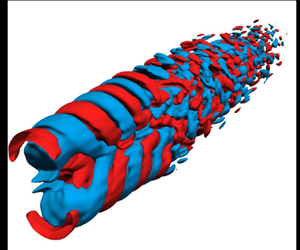
Figure 1. Computational domain on the  $x\unicode{x2013}y$ ‘in-plane’ ( $\theta = 90^{\circ }$) containing both the jets, showing the physical computational domain $\varOmega$, demarcated via a dashed boundary, and the absorbing sponge zones near the different numerical boundaries (as labelled), highlighted in grey colour. Inside the physical boundary, isocontours of vorticity magnitude $|\boldsymbol {\omega }| = 0.5U_{j}/D$ coloured by $T_{11}$ component of Lighthill's sources $|\boldsymbol{\mathsf{T}}|$ are overlaid on the dilatation field levels $\boldsymbol {\nabla } \boldsymbol {\cdot } \boldsymbol {u} = \pm 0.002U_{j}/D$ in greyscale. Solutions shown here are at a time instant corresponding to eight domain flow-through times. The polar $(r/D,\phi )$ system used to locate the far field is also shown.
Table 2. Common LES parameters for all cases of table 1.

In EFLES, flow equations are solved in generalized curvilinear coordinates via the fully compressible Navier–Stokes equations in strong conservation form (e.g. Visbal & Gaitonde Reference Visbal and Gaitonde2002). Here, spatial derivatives are discretized using an eighth-order explicit central difference scheme, while time integration is performed via an explicit three-stage third-order Runge–Kutta scheme (Kennedy & Carpenter Reference Kennedy and Carpenter1994). The time step,  $\Delta t$ (see also table 1), is chosen to satisfy $(U_j+c_\infty )\Delta t/\Delta x_{min} = 0.5$, where $\Delta x_{min}$ is the smallest grid spacing of the computational grid, which is sufficient to ensure formal numerical stability (e.g. Datta et al. Reference Datta, Mathew and Hemchandra2022). In the EFLES approach, which derives from the prior approximate deconvolution modelling (ADM) method (see e.g. Stolz, Adams & Kleiser Reference Stolz, Adams and Kleiser1999), LES modelling is accomplished by explicitly filtering the conserved variable fields in the computational space at the end of every full integration time step with an explicit central filter that is formally tenth-order accurate (Kennedy & Carpenter Reference Kennedy and Carpenter1994). The explicit filter dampens the smallest-scale motions, i.e. those corresponding to spatial wavenumbers greater than the filter cutoff wavenumber, and hence, their associated turbulent kinetic energies (TKEs). Note here that had all the flow scales been fully resolved, the TKE at scales closer to the LES filter would have naturally transferred to the smaller scales, eventually getting dissipated by the viscous processes. An LES, which does not resolve all these scales, would result in accumulation of this TKE at the smallest of flow scales, yielding steeper flow gradients and causing the simulations to eventually fail. In an EFLES, explicit filtering effectively removes this energy buildup at the smallest scales, thereby modelling the transfer of TKE from the smallest resolved scales to the unresolved scales (Mathew et al. Reference Mathew, Lechner, Foysi, Sesterhenn and Friedrich2003, Reference Mathew, Foysi and Friedrich2006; Datta et al. Reference Datta, Mathew and Hemchandra2022). Moreover, prior work with several canonical flows, including with round jets, have shown EFLES to smoothly capture the additional small-scale dynamics as the grids are refined or when the filter cutoff is raised, with no discernible change to the dynamics of the completely resolved large-scale motions.
Instead of physical nozzles, the present computations use nozzle boundary conditions specified at the inflow plane, adapted from Freund (Reference Freund2001) for twin jets by specifying
 \begin{equation} \frac{\bar{U}_x}{U_{j}} = \frac{1}{2}\sum_{k = 1}^2\left[ 1 - \tanh\left\{ b_k (\theta,t) \left(\frac{r_k}{r_0}-\frac{r_0}{r_k}\right)\right\} \right], \end{equation}
where  $\bar {U}_x$ is the time-averaged mean axial velocity, $U_{j}$ is the inflow velocity at the centreline of the jet, $r_{0}$ is the jet radius, $r_{k}$ are distances from the centrelines and $b_k$ are thickness parameters governing the thicknesses of inflow shear layers for each of the jets. In the Cartesian system,
 \begin{equation} r_{k}(y,z) = \sqrt{\left\{y + {({-}1)^k} \left( 1 + \frac{s}{D} \right) r_{0} \right\}^2 + z^2} \quad \text{for} \ k = 1,2, \end{equation}
where  $s$ is the spacing between the jets. The thickness factor $b_k(\theta,t)$ is modelled in an ad hoc manner following Freund (Reference Freund2001) by specifying a combination of azimuthal Fourier modes via
 \begin{equation} b_k\left(\theta,t\right) = 12.5 + \sum^{2}_{m=0} \sum^{2}_{n=0} A_{nm,k}\cos\left(\frac{St_{nm,k}\,U_{j}\,t}{D} + \phi_{nm,k}\right)\cos(m\theta + \psi_{nm,k}) \end{equation}
for  $k = 1, 2$, where the $nm$ subscripted parameters are now chosen via a random-walk from the range of values given in table 2, via decrementing or incrementing through its corresponding $\varDelta _{r}$ at each solution time step depending upon the outcomes of a pseudo-random-number generator. For each of the twin jets, the pseudo-random-number generators are initialized with a different random seed to ensure the inflow perturbations of these jets are nominally uncorrelated.
Our simulations were initialized via a flow field constructed by copying the reference inlet velocity and temperature profiles to every streamwise plane. The numerical solutions were allowed to evolve for five flow-through times, based on the axial domain length, or until statistically stationary turbulent jets were established (see also table 1 for  $t_{sim}$). Flow field data for calculating mean and the second-order statistics were gathered over six additional flow-through times. For this purpose, instantaneous snapshots of flow solutions were sampled at $\Delta t = 73.2 \times 10^{-3} D/U_{j}$ over five flow-through times, which corresponds to a Strouhal number $St = 13.66$, to calculate the acoustic sources that are used to extract the coherent structures and investigate sound radiation mechanisms. Our computations typically required 500 compute nodes with 24 cores per node in a supercomputer, involving a run time of approximately two days for computing ten flow-through times for each of the cases in table 1.
2.2. Far-field sound computations
In the hybrid approach followed in this work, the sources of aeroacoustic sound and its propagation need to be separately identified. While there are several ways to achieve this, the most famous approach is via an acoustic analogy where the sound is computed by solving an inhomogeneous wave equation acting on equivalent sources of sound. Lighthill's was the first such acoustic analogy (Lighthill Reference Lighthill1952, Reference Lighthill1954), where sound propagation is via a homogeneous-medium scalar wave operator acting on perturbations of density (or pressure  $p'$). This defines an equivalent acoustic source $\boldsymbol{\mathsf{S}}$ (i.e. $S_{ij}$) as the inhomogeneous term of the wave equation
 \begin{equation} \frac{\partial^{2} \rho'({\boldsymbol x},t)}{\partial t^{2}} - c^{2}_{\infty} \frac{\partial^{2} \rho'({\boldsymbol x},t)}{\partial x_{j} \partial x_{j}} = \boldsymbol{\mathsf{S}}({\boldsymbol x},t) = \frac{\partial^{2}{\boldsymbol{\mathsf{T}}}({\boldsymbol x},t)}{\partial x_{i} \partial x_{j}}, \end{equation}
where  $\boldsymbol{\mathsf{T}}$ (i.e. $T_{ij}$) is referred to as Lighthill's stress tensor. Such an equivalent source is far from a true physical source and $\boldsymbol{\mathsf{S}}({\boldsymbol x},t)$ is known to include the effects of sound refraction, which for example is a propagation effect (e.g. Samanta et al. Reference Samanta, Freund, Wei and Lele2006). Of course, there are other analogy formulations that have attempted to overcome this by eliminating such spurious propagation physics from $\boldsymbol{\mathsf{S}}({\boldsymbol x},t)$, but the end result is usually an equation that is devoid of the simplicity of (2.4). Since the subsonic cold jets considered here exclude solid surfaces in the flow field and are expected to yield minimal entropy perturbations, Lighthill's acoustic analogy, an exact rearrangement of the corresponding governing equations, should still produce the correct sound once the sources are computed exactly, in spite of the multiple physical effects clubbed into the latter. The frequency domain representation of Lighthill's equation via a temporal Fourier transform yields the familiar Helmholtz equation
 \begin{equation} \left( \frac{\partial^{2}}{\partial x_{i} \partial x_{j}} + k^{2} \right) \hat{\rho}'\left(\boldsymbol{x},\omega\right) ={-} \frac{1}{c^{2}_{\infty}} \frac{\partial^{2} \hat{\boldsymbol{\mathsf{T}}}\left(\boldsymbol{x},\omega\right)}{\partial x_{i} \partial x_{j}}, \end{equation}
where  $k = \omega /c_{\infty }$ is the wavenumber and $\widehat {({\boldsymbol {\cdot }})}$ are the Fourier transformed quantities, which is solved using the appropriate three-dimensional free space Green's function to yield
 \begin{equation} \hat{p}'\left(\boldsymbol{x},\omega_l\right) = c^{2}_{\infty} \hat{\rho}'\left(\boldsymbol{x},\omega_l\right) = \int_{\varOmega} \hat{\boldsymbol{\mathsf{T}}}\left(\boldsymbol{y},\omega_l\right) \frac{\partial^{2}}{\partial y_{i} \partial y_{j}}\left\{ \frac{\exp(\mathrm{i}\,k_l |\boldsymbol{x}-\boldsymbol{y}|}{4 {\rm \pi}\, |\boldsymbol{x}-\boldsymbol{y}|}\right\} \,\mathrm{d} \boldsymbol{y}, \end{equation}
where  $l = -N_{\omega },\ldots, N_{\omega }$. The region $\varOmega$ is the physical portion of the LES domain, where sufficient care was taken in choosing its extents to ensure $\hat {\boldsymbol{\mathsf{T}}}$ fluctuations decay off to a negligible value $\sim O(10^{-4})$ at the domain boundaries.
In the present work, a time series of  $N_{t}=4600$ samples was collected at a Strouhal number $St=13.87$, which was then split into ensembles of size $N_{e}=200$ with a $50\,\%$ overlap yielding $N_b =$ 45 ensembles. In (2.6), using $N_{\omega } = 16$ was enough to obtain frequencies until $St = 1$, which was deemed sufficient to resolve all the frequencies relevant to jet noise in this work. Further, each individual ensemble was Hann-windowed to reduce spectral leakage, while the integral in (2.6) was computed using the standard Simpson's 1/3 rule. This procedure finally yields the power spectral density of the far-field pressure fluctuations at the observer location $\boldsymbol {x}$, at a specific frequency $\omega _l$.
2.3. Extracting coherent structures from aeroacoustic sources
In the absence of any solid surfaces such as nozzles, the spatio-temporal nature of the aeroacoustic sources, identified by Lighthill's stress tensor  $\boldsymbol{\mathsf{T}}$ in (2.4), directly determines the far-field radiation via (2.6). As one of the aims here is to obtain efficient reduced-order models of the twin-jet aeroacoustic sources to better understand their radiation characteristics, we specifically focus on the coherent nature of such aeroacoustic sources via directly modelling $\boldsymbol{\mathsf{T}}$. There are now a few techniques available to extract coherent structures from turbulent flow data, but arguably the most popular one is the proper orthogonal decomposition (POD) technique, originally attributed to Lumley (Reference Lumley1967). A particular computationally inexpensive form of POD, due to Sirovich (Reference Sirovich1987), referred to as the method of snapshots, has been the most widely used. This technique extracts spatially orthogonal coherent structures along with temporal coefficients which are, in essence, stochastic parameters. The latter makes these POD modes transparent to temporal correlations of the underlying turbulent data, and thus the resulting coherent structures are not temporally coherent. In this work, we instead employ the frequency domain version of POD, referred to as SPOD, recently popularized by Towne et al. (Reference Towne, Schmidt and Colonius2018). For a given frequency, SPOD extracts orthogonal modes ranked by their modal energy and if the flow is statistically stationary, these modes together optimally represent the spatio-temporal coherence of the aeroacoustic sources. The SPOD formalism we employ in this work mostly follows Towne et al. (Reference Towne, Schmidt and Colonius2018) albeit with a few modifications which we discuss in the following paragraphs.
Before describing our SPOD method in detail, we note here that in all prior investigations with SPOD to study coherent structures in turbulent round jets (e.g. Schmidt et al. Reference Schmidt, Towne, Rigas, Colonius and Brès2018; Pickering et al. Reference Pickering, Rigas, Nogueira, Cavalieri, Schmidt and Colonius2020; Kaplan et al. Reference Kaplan, Jordan, Cavalieri and Brès2021), such structures were extracted from the primitives, while our approach here is to extract them directly from the sound sources  $\boldsymbol{\mathsf{T}}$ of (2.4) with the advantage of a more accurate description of potentially radiating structures. This may be understood from the fact that in acoustic analogies, the far-field sound pressure is directly related to the corresponding source terms, so that a superposition of various components of Lighthill's stress tensors $\boldsymbol{\mathsf{T}}$ yield the total sound. Hence, each of the SPOD modes of $\boldsymbol{\mathsf{T}}$, once computed, also has a well-defined contribution to the far-field sound via their respective linear superpositions. Such a direct and accurate physical interpretation between the reconstituted far-field sound and the spatio-temporal near-field structures is lost if the modal decomposition is first performed in terms of the primitives, subsequently used to construct the $\boldsymbol{\mathsf{T}}$ and hence the sound. We use the $\boldsymbol{\mathsf{T}}$-derived SPOD modes to construct empirical reduced-order models to carry out a systematic investigation of their radiating characteristics, which is still lacking for any kind of turbulent round jets, including, of course, twin jets considered here. Now, considering the fact that we extract SPOD modes from Lighthill's stress tensor rather than primitives, it is important to note that we seek modes that optimally represent the dataset via a standard $L_{2}$ norm as described below. This is, as opposed to using any other specialized user-defined norms, such as the induced compressible energy norm of Chu (Reference Chu1965), one of the widely used norms for compressible flows that is appropriate when extracting SPOD modes from the primitives. In addition, since $\boldsymbol{\mathsf{T}}$ is symmetric, we only extract SPOD modes for its six distinct components instead of all nine. Further, we also attempt the rather difficult task of recovering the radiated sound in the far field from our reconstructed Lighthill sources-based reduced-order models, and benchmark them against our LES-computed results, for all the cases of table 1.
Although investigations that perform aeroacoustic source reconstruction using SPOD or study the radiating characteristics of wavepackets educed from SPOD are largely missing, there are many that have attempted this using the popular snapshots-based POD, discussed above. For example, Freund & Colonius (Reference Freund and Colonius2009) applied snapshots-based POD to flow-field data obtained from the DNS of a Mach  $0.9$ jet (identical to case S in table 1) using a TKE-based $L_{2}$ norm among others. Unlike our approach, they do not use Lighthill's stress tensor $\boldsymbol{\mathsf{T}}$ to construct their POD modes but rather use the primitive fluctuating pressure data to educe wavepackets via POD, while the far-field radiation was predicted using a Kirchhoff surface based approach. Although the dominant POD modes demonstrated a wavepacket structure, it required a large number of modes ( $500$ per azimuthal wavenumber) to reconstruct the far field to be within ${\sim }4$ dB of the peak sound. A specialized norm constructed to give more weight to the far-field simulation data helped, which was able to reconstruct the far-field spectra via far fewer modes but these yielded rather poor representations of the near-field hydrodynamics. In other works, Sinha et al. (Reference Sinha, Rodríguez, Brès and Colonius2014) obtained wavepackets, also via snapshots-based POD, which were applied to perfectly expanded isothermal and moderately heated Mach $1.5$ supersonic jet data, obtained from LES. Here too, a Kirchhoff surface was used to predict the far-field radiation from POD modes, which showed good agreement at peak sound frequencies but significant underpredictions elsewhere. A similar approach was also taken by Kerhervé et al. (Reference Kerhervé, Jordan, Cavalieri, Delville, Bogey and Juvé2012), where their snapshots-based POD was conditioned with respect to an acoustically weighted energy norm.
To perform SPOD on  ${\boldsymbol{\mathsf{T}}}$, the primitives $\boldsymbol {q} = [\rho, u, v, w, p]^{\text {T}}$ from the LES in the Cartesian system are first interpolated using tri-linear interpolation onto a cylindrical grid $(r,\theta,z)$ of size $N_{r} \times N_{\theta } \times N_z =141 \times 321 \times 451$, whose centreline coincides with the $x$-axis of the LES domain. Each element of the time series data $\boldsymbol{\mathsf{T}}({\boldsymbol x}, t)$ is then decomposed azimuthally into its Fourier azimuthal components
 \begin{equation} \boldsymbol{\mathsf{T}}({\boldsymbol x},t) = \sum_{m={-}\infty}^{\infty} \boldsymbol{\mathsf{T}}^{m}(r,z,t) \exp({\mathrm{i} m\theta}), \end{equation}
where we consider  $2N_{m} + 1$ azimuthal modes ranging from $m = -N_{m}$ to $m = N_{m}$. Here, we chose $N_{m}=10$ as this was the minimum number of azimuthal modes required to faithfully reproduce the far-field spectra within $1$ dB of the LES-predicted sound at all the frequencies for all the three cases of table 1 on reconstructing $\boldsymbol{\mathsf{T}}(r,\theta,z,t)$ from $\boldsymbol{\mathsf{T}}^m(r,z,t)$. In (2.7), $\theta$ is defined as in figure 1. After removing the temporal means, each of the azimuthal Fourier components $\boldsymbol{\mathsf{T}}^{m}(r,z,t)$ are in turn decomposed into their Fourier spectral components via
 \begin{equation} \boldsymbol{\mathsf{T}}^{m}(r,z,t) =\frac{1}{2{\rm \pi}} \int_{-\infty}^{\infty} \hat{\boldsymbol{\mathsf{T}}}^{m}(r,z;\omega) \exp({\mathrm{i} \omega t})\, {\mathrm d}\omega, \end{equation}
achieved by dividing the collected time series data into  $N_{b}=45$ ensembles with a $50\,\%$ overlap in each ensemble block (for all cases in table 1, see also the discussion below (2.6)) so that the Fourier coefficient corresponding to the $k$th ensemble may be denoted as $\hat {\boldsymbol{\mathsf{T}}}^{m}_{(k)}(r,z;\omega )$. How this transformed quantity $\hat {\boldsymbol{\mathsf{T}}}^{m}_{(k)}(r,z;\omega )$ is used here to construct the cross-spectral density (CSD) matrix and obtain the SPOD modes via solving the corresponding eigenvalue problem is different from the approach of Towne et al. (Reference Towne, Schmidt and Colonius2018), the latter was also followed in other works (see e.g. Schmidt et al. Reference Schmidt, Towne, Rigas, Colonius and Brès2018; Pickering et al. Reference Pickering, Rigas, Nogueira, Cavalieri, Schmidt and Colonius2020; Kaplan et al. Reference Kaplan, Jordan, Cavalieri and Brès2021), which we elaborate now. Before that, we note that this different approach here is due to our primary objective being to construct models that accurately capture the far-field sound from twin jets, for which it was realized that preserving the three-dimensionality of the wavepackets in the calculated SPOD modes would be of utmost importance. Further, such twin-jet configurations also lack azimuthal symmetry. Hence, the need for such an approach here is at least twofold.
(i) For two-dimensional wavepackets, the usual approach (e.g. in Schmidt et al. Reference Schmidt, Towne, Rigas, Colonius and Brès2018; Pickering et al. Reference Pickering, Rigas, Nogueira, Cavalieri, Schmidt and Colonius2020; Kaplan et al. Reference Kaplan, Jordan, Cavalieri and Brès2021) is to construct a separate CSD matrix using data from each $m\unicode{x2013}\omega$ pair of the transformed quantity. This yields a CSD matrix that is devoid of the information pertaining to all other azimuthal modes necessary to capture the three-dimensional nature of the wavepackets. In our case, such an approach would not have captured the three-dimensionality of our Lighthill's stress tensor-based reduced-order model, as there is no obvious way to preserve it if reconstructed from SPOD modes obtained in this manner.
(ii) Since there is expected to be no azimuthal symmetry in twin jets, a large number of such ‘azimuthal’ modes would be needed to fully represent the dynamics, which in any case lack physical interpretation in geometries such as ours that are azimuthally inhomogeneous.

Had our objective been to solely compute single jets, none of the above points would be deemed necessary and this different approach would be redundant. Keeping these points in mind and the fact that working with the full three-dimensional LES dataset in the physical space would be computationally prohibitive, we instead retain a total of  $2N_m + 1$ azimuthal modes in the matrix ${\boldsymbol{\mathsf{Q}}}_{\omega }$, defined as
 \begin{equation}
{\boldsymbol{\mathsf{Q}}}_{\omega} = \begin{bmatrix}
\hat{\boldsymbol{\mathsf{T}}}^{{-}N_m}_{(1)} &
\hat{\boldsymbol{\mathsf{T}}}^{{-}N_m}_{(2)} &
\hat{\boldsymbol{\mathsf{T}}}^{{-}N_m}_{(3)} & \cdots
& \hat{\boldsymbol{\mathsf{T}}}^{{-}N_m}_{(N_{b})},\\
\hat{\boldsymbol{\mathsf{T}}}^{-(N_m-1)}_{(1)} &
\hat{\boldsymbol{\mathsf{T}}}^{-(N_m-1)}_{(2)} &
\hat{\boldsymbol{\mathsf{T}}}^{-(N_m-1)}_{(3)} &
\cdots &
\hat{\boldsymbol{\mathsf{T}}}^{-(N_m-1)}_{(N_{b})}\\
\vdots & \vdots & \vdots & \ddots & \vdots \\
\hat{\boldsymbol{\mathsf{T}}}^{N_m}_{(1)} &
\hat{\boldsymbol{\mathsf{T}}}^{N_m}_{(2)} &
\hat{\boldsymbol{\mathsf{T}}}^{N_m}_{(3)} & \cdots &
\hat{\boldsymbol{\mathsf{T}}}^{N_m}_{(N_{b})}\\
\end{bmatrix},
\end{equation}
\begin{equation}
{\boldsymbol{\mathsf{Q}}}_{\omega} = \begin{bmatrix}
\hat{\boldsymbol{\mathsf{T}}}^{{-}N_m}_{(1)} &
\hat{\boldsymbol{\mathsf{T}}}^{{-}N_m}_{(2)} &
\hat{\boldsymbol{\mathsf{T}}}^{{-}N_m}_{(3)} & \cdots
& \hat{\boldsymbol{\mathsf{T}}}^{{-}N_m}_{(N_{b})},\\
\hat{\boldsymbol{\mathsf{T}}}^{-(N_m-1)}_{(1)} &
\hat{\boldsymbol{\mathsf{T}}}^{-(N_m-1)}_{(2)} &
\hat{\boldsymbol{\mathsf{T}}}^{-(N_m-1)}_{(3)} &
\cdots &
\hat{\boldsymbol{\mathsf{T}}}^{-(N_m-1)}_{(N_{b})}\\
\vdots & \vdots & \vdots & \ddots & \vdots \\
\hat{\boldsymbol{\mathsf{T}}}^{N_m}_{(1)} &
\hat{\boldsymbol{\mathsf{T}}}^{N_m}_{(2)} &
\hat{\boldsymbol{\mathsf{T}}}^{N_m}_{(3)} & \cdots &
\hat{\boldsymbol{\mathsf{T}}}^{N_m}_{(N_{b})}\\
\end{bmatrix},
\end{equation}
of size  $N_{d} \times N_b$, where $N_{d}= N_{r} \times (2N_m + 1) \times N_{z} \times 6$, and use it to construct a cross-spectral density matrix ${\boldsymbol{\mathsf{X}}}_{\omega }$ (of size $N_{d} \times N_{d}$) given by
 \begin{equation} {\boldsymbol{\mathsf{X}}}_{\omega} = {\boldsymbol{\mathsf{Q}}}_{\omega}{\boldsymbol{\mathsf{Q}}}_{\omega}^{\text{H}}, \end{equation}
where  $({\cdot })^{\text {H}}$ denotes the conjugate transpose. Here, $N_{d}\sim 8 \times 10^{6}$, given that $N_r=141$, $N_m=10$ and $N_z=451$. The SPOD modes are then obtained by performing an eigenvalue decomposition on $\boldsymbol{\mathsf{X}}_{\omega }$ such that
 \begin{equation} {\boldsymbol{\mathsf{X}}}_{\omega} = \pmb{\varPhi}_{\omega} \pmb{\varLambda}_{\omega} \pmb{\varPhi}_{\omega}^{{-}1}, \end{equation}
where  $\pmb {\varLambda }_{\omega } = \text {diag}({\lambda }^{(1)}_{\omega },{\lambda }^{(2)}_{\omega },{\lambda }^{(3)}_{\omega },\ldots,\lambda _{\omega }^{(N_{d})})$ are the eigenvalues of the matrix ${\boldsymbol{\mathsf{X}}}_{\omega }$, quantifying the energies of individual SPOD modes, arranged in decreasing order by convention, while $\pmb {\varPhi }_{\omega } = [\pmb { \phi }^{(1)}_{\omega }, \ \pmb {\phi }^{(2)}_{\omega }, \pmb {\phi }^{(3)}_{\omega },\ldots,\pmb {\phi }^{(N_{d})}_{\omega }]$ are the corresponding eigenvectors, or simply the SPOD modes, at frequency $\omega$. Since the size of ${\boldsymbol{\mathsf{X}}}_{\omega }$ is prohibitively large, we construct the modified cross-spectral density matrix, $\hat {{\boldsymbol{\mathsf{X}}}}_{\omega }$, of size $N_{b} \times N_{b}$,
 \begin{equation} \hat{{\boldsymbol{\mathsf{X}}}}_{\omega} = {\boldsymbol{\mathsf{Q}}}_{\omega}^{\text{H}} {\boldsymbol{\mathsf{Q}}}_{\omega}, \end{equation}
which shares the same non-zero eigenvalues as  ${\boldsymbol{\mathsf{X}}}_{\omega }$ (see Towne et al. Reference Towne, Schmidt and Colonius2018). Eigenvalue decomposition of $\hat {{\boldsymbol{\mathsf{X}}}}_{\omega }$ yields
 \begin{equation} \hat{{\boldsymbol{\mathsf{X}}}}_{\omega} \pmb{\varTheta}_{\omega} = \pmb{\varTheta}_{\omega} {\pmb{\hat{\varLambda}}}_{\omega}. \end{equation}
 From the above equation,  $\pmb {\varPhi }_{\omega }$ can be obtained as
 \begin{equation} \pmb{\varPhi}_{\omega} = {\boldsymbol{\mathsf{Q}}}_{\omega} \pmb{\varTheta}_{\omega} {\pmb{\hat{\varLambda}}}_{\omega}^{{-}1/2}, \end{equation}
which computes the first  $N_{b}$ dominant eigenvectors of ${\boldsymbol{\mathsf{X}}}_{\omega }$. In our approach, each SPOD mode $\pmb {\phi }^{(n)}_{\omega }$ consists of the $2N_{m}+1$ azimuthal components. Hence, for the $k$th ensemble, the basis coefficient for the $n$th SPOD mode $a^{(n)}_{(k)}$ at frequency $\omega$ can be obtained as
 \begin{equation}
a^{(n)}_{(k)}(\omega) = \begin{bmatrix}
\hat{\boldsymbol{\mathsf{T}}}^{{-}N_m}_{(k)} \\
\hat{\boldsymbol{\mathsf{T}}}^{-(N_m-1)}_{(k)} \\
\vdots \\
\hat{\boldsymbol{\mathsf{T}}}^{N_m}_{(k)}
\end{bmatrix}^{\text{H}} \pmb{\phi}^{(n)}_{\omega},
\end{equation}
\begin{equation}
a^{(n)}_{(k)}(\omega) = \begin{bmatrix}
\hat{\boldsymbol{\mathsf{T}}}^{{-}N_m}_{(k)} \\
\hat{\boldsymbol{\mathsf{T}}}^{-(N_m-1)}_{(k)} \\
\vdots \\
\hat{\boldsymbol{\mathsf{T}}}^{N_m}_{(k)}
\end{bmatrix}^{\text{H}} \pmb{\phi}^{(n)}_{\omega},
\end{equation}
which therefore yields the transformed quantity  $\hat {\boldsymbol{\mathsf{T}}}^{m}_{(k)}(r,z;\omega )$ in our approach as
 \begin{equation} \hat{\boldsymbol{\mathsf{T}}}_{(k)}^{m}(r,z;\omega) = \sum^{N_{b}}_{n=1} a^{(n)}_{(k)}(\omega) \pmb{\phi}^{(n)}_{\omega}(r,m,z;\omega), \end{equation}
and thus
 \begin{equation} \hat{\boldsymbol{\mathsf{T}}}_{(k)}(r,\theta,z;\omega) = \sum_{m={-}N_{m}}^{N_{m}} \sum^{N_{b}}_{n=1} a^{(n)}_{(k)}(\omega) \pmb{\phi}^{(n)}_{\omega}(r,m,z;\omega) \exp(\mathrm{i} m\theta). \end{equation}
A reduced-order version of  $\hat {\boldsymbol{\mathsf{T}}}_{(k)}$, denoted as $\breve {\boldsymbol{\mathsf{T}}}_{(k)}$, is constructed by using $N_{s}(< N_b)$ SPOD modes, via
 \begin{equation} \breve{\boldsymbol{\mathsf{T}}}_{(k)}(r,\theta,z;\omega) = \sum_{m={-}N_{m}}^{N_{m}} \sum^{N_{s}}_{n=1} a^{(n)}_{(k)}(\omega) \pmb{\phi}^{(n)}_{\omega}(r,m,z;\omega) \exp(\mathrm{i} m\theta), \end{equation}
at each frequency  $\omega$ for the $k$th ensemble. The reduced-order model thus calculated in (2.18) is a coherent structures-based Lighthill's stress tensor model, which is now used to predict the radiation to the far field via directly substituting it in (2.6).
In the work reported here and for all the cases in table 1, the size of the matrix  ${\boldsymbol{\mathsf{Q}}}_{\omega }$, as defined in (2.9), is approximately $(8 \times 10^{6}) \times 45$, which used ${\sim }6$ GB of RAM in a MATLAB code written to compute the SPOD modes. Post azimuthal and temporal Fourier decompositions, such SPOD computations beginning with construction of $\boldsymbol{\mathsf{Q}}_{\omega }$, performing the eigen decomposition, and then writing out the SPOD modes and eigenvalues took approximately five minutes for a single frequency.
3. Spectral characteristics of twin turbulent jets
In this section, we describe the near-field turbulence and the far-field sound for the three cases of table 1 via focusing on their respective spectral characteristics. The results from twin-jet cases T1 and T2 are compared with the single-jet case S. Detailed analyses of the near-field velocity and pressure fluctuations spectra are in § 3.2, while the sound pressure spectra are in § 3.3, with some of our single-jet results benchmarked against the experiments of Stromberg et al. (Reference Stromberg, McLaughlin and Troutt1980) and the DNS of Freund (Reference Freund2001, Reference Freund2003). Further, more detailed results from our LES computations for all three cases including mean flow fields and turbulent stresses are described and compared in Appendix A while the far-field sound polar directivities are shown in Appendix B.
3.1. Instantaneous flow fields
Before showing detailed near- and far-field results, an overview of our numerical computations is demonstrated in figures 1 and 2 for both the single- and twin-jet configurations. Figure 2 shows the coloured isocontours of vorticity magnitude, depicting the jet breakdown and their subsequent evolution into turbulent structures downstream, thereby highlighting the near-field hydrodynamics which are also potential sources of the aeroacoustic sound. This is overlaid on the greyscale dilatation fields that depict the acoustic radiation to the far field from these near-field sound sources, which appear to emanate from the vicinity of their respective breakdown locations. As expected, in both cases, the strongest radiation appears to be at shallow angles (as per the polar coordinates defined in figure 1) to the jet downstream axis.

Figure 2. Instantaneous isocontours of vorticity magnitude  $|\boldsymbol {\omega }| = 0.5U_{j}/D$ coloured by the $T_{11}$ component of Lighthill's sources $\boldsymbol{\mathsf{T}}$ are overlaid on the dilatation field levels $\boldsymbol {\nabla } \boldsymbol {\cdot } \boldsymbol {u} = \pm 0.002U_{j}/D$ in greyscale, shown for (a) case S, (b) case T1, while case T2 appears in figure 1. The physical domain shown here is marked via dashed lines in figure 1 which is of size $17D\times 13D$, positioned symmetrically about the domain centreline.
3.2. Velocity and pressure fluctuations spectra
The power spectral density (PSD) of the the three components of velocity fluctuations and the pressure fluctuations are shown in figure 3 for the three cases of table 1 at three representative streamwise locations. The first streamwise location corresponds to the merger location  $x_m/D$ of case T1 ( $x=5.2D$), while the second location corresponds to the $x_m/D$ of case T2 ( $x=9.6D$). A third location, further downstream, at $x=13D$ is also studied. Here, for case S, a radial location of $r=D/2$ from the jet centreline is chosen, while for the twin-jet cases, this radial location is selected on the inner shear layer at $r=s/2$ from the jet centreline in the in-plane ( $\theta =90^{\circ }$; see figure 1). The merging of the jets is expected to alter the large-scale dynamics of the individual single jets, along with their corresponding evolution of finer-scale turbulence, which we aim to investigate in this section along with the corresponding spectra from our case S single-jet computations. Here, the PSD is computed using the Welch's method, with a cutoff frequency of $St=2$. The pressure PSD data, for example, are within an uncertainty value of $2.5$ dB at $95\,\%$ confidence interval (e.g. Bendat & Piersol Reference Bendat and Piersol2011).

Figure 3. Power spectra of the velocity fluctuations (a–c)  $u_{x}$; (d–f) $u_{r}$; (g–i) $u_{\theta }$ and ( j–l) pressure fluctuations $p$, computed at (a,d,g, j) $r/D=0.5$ for case S, and at the inner shear layer $r/s=0.5$ for the twin-jet cases (b,e,h,k) T1 and (c, f,i,l) T2, shown at three streamwise locations ——, $x/D = 5.2$; – – –, $x/D = 9.6$ and – ${\cdot }$ – ${\cdot }$, $x/D = 13$. The first two locations correspond to the merging of the twin-jet cases T1 and T2, respectively. The slope of energy cascade corresponding to isotropic turbulence is indicated via dotted lines. The radial location $r$ is with respect to the domain centreline.
For the PSD results of case S, as shown in figure 3(a,d,g, j), the first streamwise location at  $(x/D,r/D) = (5.2,0.5)$ is upstream of its potential core breakdown location $x_b = 7.3D$ (see table 1). In initially laminar jets, this region is associated with the formation and development of vortex rings, which can be mathematically modelled via linear stability waves, before their eventual breakdown due to azimuthal instabilities near $x = x_b$ (see e.g Widnall & Tsai Reference Widnall and Tsai1977; Balakrishna, Mathew & Samanta Reference Balakrishna, Mathew and Samanta2020). The large-scale dynamics at this streamwise location is therefore largely tonal for the single jet, at a single dominant frequency $St = 0.34$, as observed in the spectra of figure 3(a,d, j), corresponding to the primary velocity components and pressure, respectively, consistent with similar observations elsewhere (e.g Stromberg et al. Reference Stromberg, McLaughlin and Troutt1980; Bogey, Bailly & Juvé Reference Bogey, Bailly and Juvé2003; Bogey & Sabatini Reference Bogey and Sabatini2019). This LES-calculated PSD peak at $St=0.34$ for the single jet is close to the linear instability mode with the highest growth rate at $St=0.4$, as calculated using the analysis of Michalke (Reference Michalke1984) for the single jet of Stromberg et al. (Reference Stromberg, McLaughlin and Troutt1980), identical to ours. The small discrepancy between these results may be attributed to the differences in shear layer thicknesses between our LES and the experiments, as the frequency-dependent modal growth rates are known to be very sensitive to the thickness of shear layers. Next, results for the twin-jet case T1, which merges at this first streamwise location, are shown in figure 3(b,e,h,k). Since these jets merge before their individual breakdown locations, the coherent large-scale dynamics via the development and growth of vortex rings get disrupted which means the strong tonal peak observed for the pressure spectra in case S almost disappears in figure 3(k). Further, as the peak pressure fluctuations drop by almost an order of magnitude, this also points to weaker flow instabilities in the twin-jet case T1, upstream of the breakdown location when compared with that of case S. As for the velocity spectra, the peak PSD values between the cases S and T1 appear to be comparable, although the spectra of the latter are much more broadband in nature, especially at the higher frequencies that are more energetic than the single jet. This is the direct consequence of the jet merger happening in case T1 that introduces a cascade of finer energetic scales into the flow dynamics, which yields a jet that is more turbulent than that in case S, even before its breakdown location. Curiously, this leads to the emergence of the inertial subrange right at this first location for case T1 (see, especially figure 3b,e) where the spectra are expected to follow the slope of energy cascade in isotropic turbulence, i.e. $-5/3$ for velocity and $-7/3$ for pressure fluctuations, near the cutoff frequency of $St = 2$. For the case T2 twin jet, which merges downstream of this first streamwise location, the curves in figure 3(c, f,i,l), unsurprisingly, show close resemblance to the corresponding curves of case S, with an identical tonal peak at $St = 0.34$.
The second streamwise location at  $(x/D,r/s) = (9.6,0.5)$, where the case T2 twin jet merges, is beyond the single-jet breakdown location and therefore all the jets are already fully turbulent at this point as evidenced from this location's spectra that show approximate match with the respective inertial subrange energy cascade slopes. Here the spectra seem to shift toward lower frequencies and show more broadband features with higher fluctuations over a broader range of $St$ (see Ball, Fellouah & Pollard Reference Ball, Fellouah and Pollard2012; Brès et al. Reference Brès, Jordan, Jaunet, Le Rallic, Cavalieri, Towne, Lele, Colonius and Schmidt2018) for all the cases studied, including that for the single-jet case S (see figure 3a,d,g, j). Across the velocities and pressure, the spectra now show similar shapes and frequency content. However, for the twin-jet case T1, which was already turbulent further upstream near its merger, the change in its spectra at this second streamwise location is minimal (see figure 3b,e,h,k).
The third streamwise location at  $(x/D,r/s) = (13,0.5)$ is further downstream, by which point the turbulence has started to decay, although the shape of the various spectra remain approximately similar to the second location. The twin-jet case T2 show a larger decay in its pressure fluctuations (see figure 3l) at this location, approaching that of the closely spaced twin-jet case T1 over a broad range of low frequencies.
3.3. Sound pressure spectra
The far-field pressure fluctuations representing the aerodynamic sound appears in figure 4 for a few selected polar angles  $\phi$ on the in-plane ( $\theta = 90^{\circ }$) and cross-planes ( $\theta = 0^{\circ }$). Figure 4 shows the far-field pressure spectra, with the pressure computed via the solution to Lighthill's acoustic analogy in (2.6) at several spatial locations $\boldsymbol {x}$ and frequencies $St$. Here, the spatial locations are expressed in a spherical coordinate system $(r,\theta,\phi )$, convenient to locate the far field of twin jets, where $\theta$ is the angle that locates the specific plane about the geometric centreline of the configuration while $(r,\phi )$ are simply the polar coordinates on that two-dimensional plane (see figure 1 for the coordinate system). Although for case S it is immaterial, for the twin-jet cases T1 and T2, $\theta =90^{\circ }$ is the plane containing both jets, hence referred to as the ‘in-plane’, while the ‘cross-plane’ is normal to it at $\theta =0^{\circ }$. The radial distance for all the far-field results is fixed at $r/D=30$, after accounting for the virtual origin of the respective jets (see figure 1). Further, in figure 4, we also compare the far-field results of our case S with the DNS of Freund (Reference Freund2001) and the experiments of Stromberg et al. (Reference Stromberg, McLaughlin and Troutt1980) for which data at only the downstream angle of $\phi = 30^{\circ }$ are available.

Figure 4. The far-field pressure spectra at locations on the (a)  $\theta =90^{\circ }$, in-plane and (b) $\theta =0^{\circ }$, cross-plane at a distance of $r/D=30$ from the virtual origin and at several polar angles $\phi =30^{\circ }, 60^{\circ }, 90^{\circ }, 120^{\circ }$ and $150^{\circ }$ shown for (– ${\cdot }$ – ${\cdot }$, grey) case S; (——, red) case T1 and (– – –, blue) case T2 of table 1. In panel (a), at $\phi = 30^{\circ }$, data from the DNS of Freund (Reference Freund2001) and the measurements of Stromberg et al. (Reference Stromberg, McLaughlin and Troutt1980) are also included as solid black line and black circles, respectively. The grey band represents a deviation of ${\pm }3$ dB from the single-jet spectra, the vertical dash-dotted line indicates $St =0.14$ and the dashed line shows $St=0.34$.
In contrast to the near-field hydrodynamic spectral peak at  $St=0.34$ (see figure 3j,l), the far-field spectra show a distinct peak at $St=0.14$, which is more clearly seen at the shallow angle $\phi =30^{\circ }$ for both the in-plane and cross-plane orientations and for all the jets studied here (see the topmost plots of figures 4a and 4b, respectively). At the other angles, sideline and upstream, as the sound spectra become more broadband due to radiation from the small-scale turbulence as the spectra even out over the lower frequencies, this spectral peak at $St=0.14$ becomes less prominent and almost disappears at $\phi = 150^{\circ }$, the most upstream radiation direction shown. At $\phi = 30^{\circ }$, the sound pressure spectra from our computed case S shows good match with the experiments of Stromberg et al. (Reference Stromberg, McLaughlin and Troutt1980) (see the topmost plot of figure 4a), which has been shifted here vertically to align at the higher frequencies. Further, the peak radiation at $St=0.14$ matches with the results of Freund (Reference Freund2003) too, obtained via a DNS and the application of Lighthill's equation, while the peak amplitudes are within 2 dB of each other. Such impressive match with the available DNS and experimentally measured spectra for the single jet also confirm our numerics to be correct, both in the LES and Lighthill's solvers. Note here that for the single-jet case S, the in-plane and cross-plane spectra should be ideally identical at a given $\phi$, but there are minor noticeable differences in figure 4(a,b), which could have been eliminated via gathering more ensembles from longer time series data in our LES calculations, which we decided not to pursue here. In fact, the only significant differences observed is at $\phi = 60^{\circ }$, near the spectral peak, which is of the order of $3$ dB but everywhere else, i.e. at all other polar angles and frequencies, such differences between in-plane and cross-plane data are negligibly small.
Moving on to the twin-jet results, the first thing to note in figure 4 is the fact that twin-jet spectra identically peak at  $St=0.14$ (marked via vertical dash-dotted lines), although with different amplitudes, at all the shallow and sideline angles. This is similar to what was observed in the near-field spectra of figure 3, which peaked at $St=0.34$, at locations upstream of the jet breakdown for the single jet and also largely for the twin jets. Such a finding points to two things. First, the most energetic structures of the near field at $St=0.34$ do not necessarily radiate strongly, so that only a small fraction of the near-field energetic fluctuations contribute to radiated sound power of the far field. This is not unexpected and a simple analysis shows the hydrodynamic structures at $St=0.34$ to possess subsonic phase speeds, while those at $St = 0.14$ do indeed have supersonic phase speeds, necessary for them to radiate to the far field, as demonstrated in Appendix D. Second, closely spaced twin jets, like those considered here, do not significantly alter the frequency of peak radiation (at a given angle) in spite of the twin jets possessing significantly different mean and turbulent characteristics when compared with the constituent single jet, as shown in Appendix A, and also strikingly different coherent dynamics as we show next in § 4. Now, the fact that our twin jets radiate louder over the single jet at the same $St$ may seem to be a validation of the $+3$ dB rule, discussed in § 1, where twin jets are simply louder versions of equivalent single jets. However, as we show next, the $+3$ dB rule is a gross oversimplification for estimating twin-jet noise, whose overall spectral characteristics differ greatly from the single jet over a range of parameters.
One such important parameter, as being investigated in this work, is the effect of the twin-jet spacing distance  $s/D$. This is known to affect the radiated sound from the twin jets by modifying the phenomenon of shielding, where there is a reduction of sound levels in the plane containing the two jets (i.e. $\theta =90^{\circ }$) (see e.g Mani Reference Mani1972; Balsa Reference Balsa1975; Kantola Reference Kantola1981). According to Kantola (Reference Kantola1981), for smaller spacing between jets, such as in case T1, the effectiveness of shielding is not expected to be significant, whose effect continues to increase until $s/D=3$, after which it plateaus. In contrast, focusing on our closely spaced twin-jet case T1, the top plots of figures 4(a) and 4(b) show an increase of peak radiation at the cross-plane ( $\theta = 0^{\circ }$) compared with those of the single jet by $\sim 7$ dB, while at the in-plane ( $\theta = 90^{\circ }$), this increase is lower and approximately contained within the $\pm 3$ dB band of figure 4(a). At $\phi = 60^{\circ }$ (see the second plot of figures 4a and 4b), there is more drastic reduction of peak radiation at the in-plane angle, which seems to fall below the single-jet radiation level. Further, continuing with shallow angles, at $\phi =30^{\circ }$ for the in-plane location (see the top plot of figure 4a), there is almost a $\sim 5$ dB drop in the case T1 spectra at $St \sim 0.4$, compared with the single-jet radiation. All these are clearly due to the effect of shielding, observed here for twin jets with $s/D = 0.1$ and at the shallower angles. At the sideline and smaller upstream angles (see the third and fourth plots of figures 4a and 4b), as we move away from the jet centrelines towards sideline angles, there is less evidence of any shielding to be active for the twin jets. This behaviour may be attributed to the rather short travel time through the jet flow associated with radiation at these angles (Kantola Reference Kantola1981). At the most upstream angle $\phi = 150^{\circ }$, there is again some shielding visible (compare the bottom plots between figures 4a and 4b), which is, though minor, comparable to that at the shallow angles. Surprisingly, unlike in case T1, the further spaced twin-jet case T2 hardly shows any effect of shielding, where peak radiation at all the polar $\phi$ angles (except, perhaps at $\phi = 150^{\circ }$) remain comparable across the in-plane and cross-planes and no clear trend is observed in figure 4.
3.3.1. Investigating the $+3$ dB rule via artificially realized twin jets

One of the reasons for inserting the single-jet  ${\pm }3$ dB grey bands in figure 4 is to provide rough predictions for the twin-jet sound power amplitudes when compared with the equivalent-exit-area single jet, which has been rather widely used in the industry (see e.g. Kantola Reference Kantola1981; Brès et al. Reference Brès, Bose, Ham and Lele2014). However, as the figure 4 results for the twin-jet spectra have already shown, the $+3$ dB limit only provides a rather crude estimate, as is expected from a thumb rule, which appears to be a function of the jet separation distance. Moreover, as the twin jets merge, the process creates an extra hierarchy of scales of various sizes that are now potential sources of radiation, which the $+3$ dB rule ignores, so much so that whether the sound from these merging twin jets would follow the $+3$ dB bound is also very much a function of their frequency. Here we argue that it is this very presence of extra flow structures in the merging twin jets which yield a radiation that is different to that of equivalent single jets. This is not so much due to the jet separation distances, as may have been apparent in the above discussion, especially along cross-planes ( $\theta = 0^{\circ }$) where the effects of jet shielding are absent. To test this hypothesis, we create a pair of artificial twin jets via taking two realizations of the aeroacoustic sources from the single jet (case S), given by (2.4), which are shifted by a distance $s/D$, corresponding to cases T1 and T2 of table 1.
The far-field spectra from these artificial twin jets is now calculated and shown in figure 5 along with the physical twin and single jets for both the in-plane and cross-plane locations at a few selected polar angles. Care is taken to decorrelate the individual realizations of single-jet sources by time shifting them via one flow-through time, relative to each other. Increasing the time-shift further did not have a significant impact on the results shown. Figure 5(b) shows the far-field spectra from both these artificial twin jets to be essentially identical at the cross-plane ( $\theta = 0^{\circ }$) for all polar angles and their magnitudes largely fall at the edge of the $+3$ dB bound shown in the figure. These observations yield two outcomes. First, the effect of jet spacing on radiated sound is less significant along locations in the cross-plane, where as the spacings change, at least from the listener's perspective, the aeroacoustic sources are merely shifted along directions normal to the line connecting the sources and the listener. The second observation being at the cross-plane, such artificial jets almost faithfully follow the $+3$ dB rule over all frequencies. Hence, whatever discrepancies we observe in figure 5(b) between the spectra of cases T1 and T2 and their artificial counterparts are clearly attributable to the nature of flow structures arising from the jet interactions in the former set.

Figure 5. Far-field pressure spectra extracted from figure 4, but shown only for  $\phi = 30^{\circ }$, $90^{\circ }$ and $150^{\circ }$ for(– ${\cdot }$ – ${\cdot }$, grey) case S; (——, red) case T1 and (– – –, blue) case T2 of table 1, with additional far-field pressure spectra results shown for the artificial twin jets (see text): ( $\blacktriangle$, red) artificial case T1 and ( $\blacktriangledown$, blue) artificial case T2. (a) In-plane ( $\theta =90^{\circ }$), (b) cross-plane ( $\theta =0^{\circ }$).
Similar trends can be observed in the corresponding overall sound pressure level (OASPL) as a function of the polar angle  $\phi$ for the the cross-plane $\theta = 0^{\circ }$ (see figure 17a), shown in Appendix B. Here, differences are small and for polar angles $\phi > 90^{\circ }$, the four twin-jet curves overlap, indicating radiation to be neither a strong function of jet separation distances nor of the jet merger dynamics.
Things are slightly more complicated in the  $\theta = 90^{\circ }$ in-plane (see figure 5a), where the jet shielding is active, which we have already shown to be a function of the jet separation distance $s/D$. Here, as the source separations are varied in the artificially constructed jets, differences appear more in the higher frequencies since only for these relatively higher frequency waves, the rather small separation distances considered here are perhaps adequately resolved. Even then, the physical twin-jet spectra vary greatly from the corresponding artificial ones (up to ${\sim }8$ dB) at some $St$ values for the shallow angle $\phi = 30^{\circ }$ shown here (see the top plot of figure 5a). At these shallow angles, we have seen shielding to be more active for the closer-spaced jet case T1 which therefore yields such extra sensitivity, which disappears at the other sideline and upstream angles $\phi$ where the effects from shielding are less important. At these higher polar angles, the differences between the physical and artificial twin-jet spectra are mostly smaller, irrespective of $\theta$ planes, which may be visualized in greater detail in the OASPL plots of figure 17(b–d) in Appendix B.
To summarize, the often used single-jet  $+3$ dB rule for twin turbulent jet radiation is most likely to work at the sideline and upstream polar $\phi$ angles, largely independent of the $\theta$-plane orientations. This is in spite of the fact that the rule itself, which ignores jet interactions, is expected to work the best at the $\theta = 0^{\circ }$ cross-plane, where the effects of jet-shielding are absent.
4. Coherent aeroacoustic sources of twin jets
The results and discussion of § 3 and Appendix A have clearly established the rather different flow dynamics of the twin subsonic jets, as considered here, when compared with their constituent single jet. The separation distance  $s/D$ of the jets affect the in-plane shielding mechanism, which is mostly prevalent at low polar angles to the jet downstream, while the twin-jet merging process creates these extra scales, mostly of smaller spatial coherence, which seem to be the key differentiator in their respective sound radiation spectra, showing up over moderate to higher frequency bands. In this section, we attempt to construct reduced-order models for these jets by extracting spatio-temporally coherent three-dimensional structures (SPOD modes) following the procedure described in § 2.3. The convergence details of SPOD computations are discussed in Appendix C. Unlike other approaches, we apply this method directly to the Lighthill's stress tensor $\boldsymbol{\mathsf{T}}$ of (2.4), so that these extracted SPOD structures are nothing but spatio-temporally optimized coherent aeroacoustic sources. In § 4.1, we first describe the dynamics of these SPOD modes with respect to their eigenspectra, low-rank behaviour and mode shapes, and highlight how the twin-jet SPOD modes differ from that of the single jet. Next, in § 4.2, these modes are combined to obtain reduced-order models for the radiated sound for all the jets considered in table 1 over a range of frequencies, polar angles and jet planes, i.e. $(St,\phi,\theta )$. Note that the SPOD modes obtained here are optimized to capture the near-field coherence of the sources and these modes are in no way expected to be optimal for the sound radiated to the far field (see e.g. Freund & Colonius Reference Freund and Colonius2009; Kerhervé et al. Reference Kerhervé, Jordan, Cavalieri, Delville, Bogey and Juvé2012). In fact, in this work, we do not attempt to construct SPOD modes that are preferentially weighted for the far-field sound. Still, instead of the thousands of snapshots-based POD modes which are apparently needed to form such reduced-order models for the radiated sound, our attempt below shows only tens of three-dimensional SPOD modes (per frequency) are all that are required to construct such models with subdecibel levels of accuracy.
4.1. Dominant modes and their dynamics
4.1.1. Eigenspectra, modal energy content, low-rank behaviour
Several features of the SPOD modes computed for the cases via the procedure of § 4.1 are described in figure 6. Here, SPOD eigenvalues are depicted in two different ways. First, in figures 6(a–c) and 6(d–f), these eigenvalues are shown as a function of the mode number  $n$ (see (2.18)) at the frequencies $St=0.14$ and $St=0.34$, respectively. These SPOD eigenvalues are scaled with respect to the total energy at that frequency. The frequencies $St=0.14$ and $St=0.34$ are chosen as reference frequencies to show our results in this section, since as figures 3 and 4 have respectively shown, the near-field PSD and far-field spectra mostly peak at these frequencies for all the jets. Expectedly, at $St=0.34$, the leading mode for the single-jet case S (see figure 6d) is substantially more energetic than all the suboptimal SPOD modes, pointing to its low-rank behaviour at this frequency, where hydrodynamic fluctuations were seen to peak before (see also Schmidt et al. Reference Schmidt, Towne, Rigas, Colonius and Brès2018). The same is apparent with the first SPOD mode of case T1, at this frequency, shown in figure 6(e), while for the case T2, the further spaced twin jet does not seem to possess any dominant low-rank dynamics since its first two dominant SPOD modes have similar levels of energies (see figure 6f). At $St=0.14$, as figure 6(a–c) show, such low-rank dynamics of the case S and case T1 jet also diminish, while for the former, the first three eigenvalues seem to be significantly more energetic than the rest. So, focusing on the first three eigenvalues for all, figure 6(g–i) show the full spectra of SPOD modes over the range of frequencies, where the eigenvalues are normalized by the total modal energy integrated over the entire frequency range. The suboptimal eigenvalues are shown in shades of grey. The low-rank behaviour for the cases S and T1 are confirmed at $St=0.34$ due to the large separation between the fractions of total energy as described by the most dominant mode and the suboptimal modes in either case. This spectral peak at $St=0.34$ has been associated with the most amplified K–H instability wave, as seen in § 3.2. Further, in cases S and T2, we see the presence of a second peak for the dominant SPOD mode at $St = 0.41$ as well, which appears in the first sub-dominant SPOD mode for case T1. This is not surprising since the respective PSD results also indicated the presence of such a second peak at $St = 0.41$ for the cases S and T2 (see figure 3a,c,d, f, j,l). The absence of such an energy peak for case T1 in the dominant SPOD mode suggests the dynamics associated with the scales at $St = 0.41$ to be largely impeded due to the twin jets merging in case T1 upstream of the breakdown, although it does show up in the first suboptimal SPOD mode, as seen in figure 6(h), albeit at a much reduced fraction of the total flow energy. Finally, figure 6( j–l) show that up to $95\,\%$ of the total modal energy is easily isolated by less than $40$ of these computed three-dimensional SPOD modes for $St < 1$. Near $St = 0.34$, where the spectral peak appears, energy contributions from the dominant modes improve, although for the twin jets, this is less so, again pointing towards reduced low-rank dynamics in these jets. At higher $St$, a very large number of modes are usually needed to recover a significant fraction of the total modal energy, due to the lack of coherence in these higher- $St$ SPOD modes (Nekkanti & Schmidt Reference Nekkanti and Schmidt2021). This is not yet observed for the frequency cutoff of figure 6.

Figure 6. SPOD modes for the cases of table 1, showing SPOD eigenvalues for (a–c)  $St = 0.14$ and (d–f) $St = 0.34$ normalized by the total modal energy at $St = 0.14$ and $St = 0.34$, respectively; (g–i) SPOD eigenvalues as a function of $St$, normalized by the total modal energy integrated over the entire frequency range and ( j–l) the percentage of total energy contained in the first dominant $N_{s}$ SPOD modes as a function of frequency (in greyscale) with curves for three representative values: $60\,\%$, $80\,\%$ and $95\,\%$ highlighted. In panels (g–l), the vertical dash-dotted and dashed lines correspond to $St=0.14$ and $St=0.34$, frequencies at which the far-field and near-field spectra peak, respectively.
4.1.2. Three- and two-dimensional mode shapes
In this section and the next, we discuss the nature of SPOD modes extracted from Lighthill's sources  $\boldsymbol{\mathsf{T}}$ by focusing only on the dominant $T_{11}$ component (see discussions in Freund Reference Freund2003; Muthichur, Hemchandra & Samanta Reference Muthichur, Hemchandra and Samanta2021). SPOD modes associated with the other components of $\boldsymbol{\mathsf{T}}$ behave not too differently although the energy levels are much lower. These modes are documented elsewhere (see Muthichur Reference Muthichur2023) but all six unique components of $\boldsymbol{\mathsf{T}}$ are used to obtain the low-dimensional reconstructions as discussed in the next section.
Figure 7 shows the three-dimensional, spatio-temporally coherent  $T_{11}$ aeroacoustic sources corresponding to the three cases shown at the two frequencies $St=0.14$ and $St=0.34$ on which we focus here and also at an intermediate frequency $St=0.25$. The spatial coherence observed at $St=0.34$ is quite remarkable, especially for the twin jets (figure 7h,i), which reduce at higher $St$ (not shown here). Further, symmetrical mode shapes of the single-jet case S at this frequency (figure 7g) indicate it to be dominated by the axisymmetric $m=0$ mode, while the twin-jet cases are likely dominated by the higher azimuthal modes. This is shown in Appendix E by performing azimuthal decomposition on the individual jets in these computed three-dimensional SPOD modes. Similarly, at $St=0.14$, figure 7(a–c) suggest even the single-jet hydrodynamics to be dominated by higher order azimuthal modes.

Figure 7. Real part of the dominant three-dimensional SPOD modes for the  $T_{11}$ component of Lighthill's stress tensor $\boldsymbol{\mathsf{T}}$ shown for the cases of table 1 at (a–c) $St=0.14$; (d–f) $St=0.25$ and (g–i) $St=0.34$.
The SPOD mode shapes for  $T_{11}$ are plotted at the in-plane ( $\theta = 90^{\circ }$) for several frequencies in figures 8 and 9, showing the leading SPOD mode in all cases, while also the first suboptimal mode for the $St = 0.14$ and $St = 0.34$ cases. The raw $T_{11}$ sources, as obtained from the LES computations, are also plotted side-by-side for comparison. Overall, all the figures demonstrate some form of coherent wavepackets, more so for the single-jet case S pictures, while for the twin-jet cases T1 and T2, good to reasonable coherence are observed in the $St = 0.25, 0.34$ and $0.45$ cases. At the higher frequencies of $St=0.6$ and $0.8$ considered here (see figures 9j–l and 9m–o, respectively), the wavepacket wavelengths reduce, so do their spatial support, which therefore do not show much of coherence visually. In contrast, at $St = 0.34$, where the hydrodynamic fluctuations were seen to peak (seen discussion in § 3.2), the SPOD modes show excellent coherence, where the wavepacket structures corresponding to both the leading and first suboptimal SPOD modes of case S (see figures 8j and 8m, respectively) are aligned along the jet columns, implying the characteristics of a dominant $m=0$ mode (see Appendix E). Note that the second mode of figure 8(m) has two streamwise maxima, similar to observations elsewhere (e.g. Towne et al. Reference Towne, Schmidt and Colonius2018). At this frequency, we have seen in figures 6(e) and 6( f) respectively that the case T1 twin jet shows low-rank dynamics while the case T2 twin jet does not. This is reflected here in the modal structures of figure 8(k,n), where the leading mode for case T1 shows more coherence than the suboptimal, while after the merger location (indicated via vertical dotted lines), the leading mode even shows dominant wavepacket structures along the domain centreline, which is now the jet centreline of the merged jet, similar to figure 8( j,m). This confirms our observations (see discussion in § A.1) that the dynamics of the case T1 twin jet largely follows that of a single jet (case S), immediately downstream of the merger. As for the case T2 twin jet, figure 8(l,o) show the first two SPOD modes to be energetically similar, being approximate mirror images of each other. Upstream of the jet breakdown, at $St \gtrsim 0.3$, the wavepackets are known to be associated with the jet K–H instability (Gudmundsson & Colonius Reference Gudmundsson and Colonius2011; Schmidt et al. Reference Schmidt, Towne, Rigas, Colonius and Brès2018) (see figure 8j,k,l,o), seen here for both the single and twin jets. Beyond the jet breakdown (indicated via vertical dashed lines), the K–H instability disappears so do these SPOD wavepackets mostly. The exception here is the first suboptimal single-jet mode of figure 8(m), which peaks downstream of the breakdown, likely modelling the Orr modes of turbulent jets.

Figure 8. Spatio-temporal coherent structures of the  $T_{11}$ component of Lighthill's stress tensor $\boldsymbol{\mathsf{T}}$ on the in-plane ( $\theta = 90^{\circ }$) for the cases of table 1, showing (a–c) the dominant $T_{11}$ component from the LES computations; the corresponding SPOD eigenmodes at $St=0.14$ for (d–f) the leading mode $(n = 1)$ and (g–i) the second mode $n = 2$; and the eigenmodes at $St = 0.34$ for ( j–l) the leading mode $(n = 1)$ and (m–o) the second mode $(n = 2)$. In all figures, the horizontal dotted line is the domain centreline while for case S, it is also the jet centreline. The horizontal dashed lines indicate the respective jet centrelines for twin-jet cases T1 and T2, while the vertical dashed and dotted lines indicate the jet breakdown and merger locations, as before. The contour levels for all the figures is ${\pm }30 \times 10^{-3}.$

Figure 9. Same as in figure 8, but showing only the leading SPOD mode  $(n = 1)$ at the frequencies (d–f) $St=0.25$; (g–i) $St=0.45$; ( j–l) $St=0.60$ and (m–o) $St=0.80$. The contour levels for all the figures are ${\pm }30 \times 10^{-3}$.
At  $St=0.14$, none of the jets, especially the twin-jet cases T1 and T2, show any low-rank behaviour (see figure 6a–c). In figure 8(d), for the single jet, some presence of wavepacket structures aligned along the liplines is apparent that seem to be the most energetic upstream of the jet breakdown region, while the second mode of figure 8(g) is more dominant near and beyond this breakdown. Here, at $St=0.14$, the wavepackets aligning along the lipline indicates the dynamics at this frequency to be dominated by the $m>0$ azimuthal modes (see also the three-dimensional mode pictures in figure 7a–c), as confirmed in Appendix E. The absence of low-rank dynamics at $St=0.14$ is also reflected in the wavepacket structures of cases T1 and T2 which lack coherence and although these wavepackets appear to be localized at individual shear layers, they appear at different SPOD modes (see figure 6e, f,h,i), i.e. if the wavepackets corresponding to the top jet shear layer are more energetic in the first SPOD mode (figure 8e, f), then the bottom jet is more energetic in the second SPOD mode (figure 8h,i). This observation also points to the fact that flow dynamics at the individual jet shear layers are largely uncorrelated at this frequency. At $St \lesssim 0.3$, such wavepacket structures are expected to model non-modal dynamics of the jets (Tissot et al. Reference Tissot, Lajús, Cavalieri and Jordan2017; Schmidt et al. Reference Schmidt, Towne, Rigas, Colonius and Brès2018).
The spatial nature of the leading SPOD mode at frequencies  $St=0.25$, shown in figure 9(d–f), and $St=0.41$, shown in figure 9(g–i), for all the jet cases largely follow that of $St=0.34$ and are not elaborated further.
4.1.3. Radial and axial profiles, wavepacket nature
To further highlight the important features of SPOD modes as discussed in § 4.1.2, in this section, we show their one-dimensional radial and axial profiles in figure 10 at  $St = 0.34$. For the single-jet case S, radial profiles are shown at three axial locations in figure 10(a), corresponding to the breakdown location $x = x_b$ and at distances which are $x = 2D$ away upstream and downstream of the breakdown. As commented in § 4.1.2, the $St=0.34$ SPOD modes correspond to K–H instability modal dynamics, upstream of the jet breakdown, which is clearly observed in figure 10(a) for the radial profile at the upstream location, characterized by growth, saturation and rapid decay in the radial direction, all features of the most-amplified K–H mode (see e.g. Suzuki & Colonius Reference Suzuki and Colonius2006). Expectedly, the K–H modal dynamics rapidly decays off near the breakdown location and further downstream as also observed with the corresponding SPOD mode radial profiles at such locations. For the twin-jet case T1, at the merger location shown in figure 10(b), which is approximately the same as the $(x_b-2D)$ streamwise location of the single jet, we see the presence of a stronger second peak close to the domain centreline, which becomes the jet centreline post merger. This indicates, like we have seen in § 4.1.2 and later in § A.1, that the closely spaced twin jet behaves very much like a single jet from its merger onward, with the relevant strong K–H modal dynamics apparent along its geometric centreline. In contrast, for the case T2 twin jet that merges downstream of the breakdown, no second peak near the domain centreline is seen (see figure 10c) and the K–H dynamics shifts to the jet centreline at $y/D = 1$ (marked via the vertical dotted line), still showing the familiar growth, saturation and decay along the radial direction, albeit at a somewhat slower rate than either of cases S and T1. The corresponding SPOD radial profiles at $St = 0.14$ (not show here), especially for the twin-jet cases T1 and T2 show some signatures of Orr wavepackets, as these peak near and downstream of the breakdown, by which point the K–H-based dynamics disappears (see Schmidt et al. Reference Schmidt, Towne, Rigas, Colonius and Brès2018; Pickering et al. Reference Pickering, Rigas, Nogueira, Cavalieri, Schmidt and Colonius2020).

Figure 10. (a–c) Radial profiles and (d–f) axial profiles of leading SPOD modes of the  $T_{11}$ component at in-plane $(\theta = 90^{\circ })$ for $St=0.34$. Radial profiles are shown at streamwise locations, including ——, $x = x_b$, the respective jet breakdown locations (see table 1); – ${\cdot }$ – ${\cdot }$, $x = (x_b - 2D)$ and $\cdots$ $\cdots$, $x = (x_b+2D)$ in panel (a) for case S; – ${\cdot }$ – ${\cdot }$, $x = x_m$ and $\cdots$ $\cdots$, $x = (x_b+2D)$ in panel (b) for case T1 and – ${\cdot }$ – ${\cdot }$, $x = (x_b-2D)$ and $\cdots$ $\cdots$, $x = x_m$ in panel (c) for case T2. Axial profiles are at radial locations corresponding to jet centrelines so that ——, $r = 0$ for case S in panel (d) while —— and – ${\cdot }$ – ${\cdot }$, top and bottom jet centrelines respectively in panels (e) and ( f) for cases T1 and T2, respectively. In panel (a–c), the vertical dotted lines locate the jet centreline for the twin jet cases and in panel (d–f), the vertical dashed and dotted lines represent the jet breakdown and merger locations, respectively.
However, the streamwise variation of the SPOD modes along the jet centreline, shown in figure 10(d–f), confirms the expected oscillatory nature of the K–H wavepacket structures at  $St=0.34$ when such modes peak, bound by envelopes of growth, saturation and decay (e.g. Arndt, Long & Glauser Reference Arndt, Long and Glauser1997; Gudmundsson & Colonius Reference Gudmundsson and Colonius2011; Jordan & Colonius Reference Jordan and Colonius2013). Also, as expected from such modal dynamics, all the SPOD wavepackets peak upstream of the respective breakdown locations (indicated via vertical dashed lines) and there are only minor differences between wavepackets of each of the two constituent jets in cases T1 and T2. The corresponding axial profiles at $St=0.14$ (not shown), when the K–H modal dynamics is absent, would be less oscillatory.
4.2. Low-dimensional reconstruction of the aeroacoustic sound
In this section, we focus on our stated primary objective in § 1, which is to construct accurate reduced-order models for the sound radiated from twin subsonic jets. In many ways, such a model reconstructed from the aeroacoustically relevant sources present in twin jets is not expected to be straightforward since, as we observed in the discussion of § 3, unlike for single jets, the dynamics of twin-jet evolution also depends on their merger location  $x_m/D$ (and hence their separation distance $s/D$) apart from the jet breakdown location $x_b/D$. Further, the spatio-temporally coherent twin-jet SPOD modes of § 4.1 are seen to show rather poor low-rank behaviour, especially at $St=0.14$ where the peak sound is observed in our LES calculations (see figure 6a–c). The corresponding spatial structures of these modes do not show strong coherence either (see figure 7a–c), while the complex nature of flow structures in twin jets point to the need of a rather large number of modes to reconstruct the far-field sound to be within a decibel of that predicted by the actual LES calculations. However, at $St = 0.34$, some low-rank character for the twin jets is still evident in figure 6(e, f), especially for the case T1 twin jet, but also for the further-spaced case T2 twin jet considering that its constituent jets evolve largely independently for a significant length. To get some idea on what has been achieved so far with the far-field sound reconstruction from model sources in jets, we note that Freund & Colonius (Reference Freund and Colonius2009) using their snapshots-based POD needed $9500$ two-dimensional modes to be close to $4$ dB of the peak sound from their $M_j=0.9$ single jet. Pickering et al. (Reference Pickering, Towne, Jordan and Colonius2021), however, used the so-called acoustic resolvent modes, where the resolvent output included the purely acoustic fluctuations of the far field, further enhanced via an eddy-viscosity model. Such a leading acoustic resolvent mode, taking advantage of the low-rank dynamics for their $M_j=0.9$ single jet, was able to obtain the correct peak sound within $2$ dB via the use of five such modes in conjunction with a source model. However, the angle $\phi$ at which sound from their resolvent model peaked was slightly off from the LES predicted sound.
In this work, our calculated SPOD modes are not optimized for the far-field sound which, quite expectedly, yield a sound that falls well short from the LES predicted sound, as observed in figure 11 at the in-plane  $\theta = 90^{\circ }$, shown here only for the leading three SPOD modes (as highlighted in figure 6g–i). Larger differences are observed at $St = 0.14$, which are close to $40$ dB at some polar $\phi$ angles, while at $St=0.34$, differences are less, presumably because of the better low-rank dynamics of leading modes at this frequency, although it is still ${\sim }10$ dB less than the LES predicted sound at most of the polar angles highlighted in figure 11(d–f). Out of the three leading SPOD modes shown here, surprisingly, the first SPOD mode shows the most error in its radiated sound for the single jet and the case T2 twin jet. Such an observation again points to the fact that SPOD modes obtained via standard near-field-based $L_2$ norm, like ours, are unlikely to be optimal with respect to the radiated sound.

Figure 11. Far-field sound pressure level (SPL) on in-plane ( $\theta =90^{\circ }$) from the three leading SPOD modes (——, $n=1$; – – –, $n=2$ and $\cdots$ $\cdots$, $n=3$) of $\boldsymbol{\mathsf{T}}$ compared with the sound from LES (——, black), shown for (a,d) case S; (b,e) case T1 and (c, f) case T2 of table 1. The two frequencies of interest are (a–c) $St = 0.14$ and (d–f) $St=0.34$, as before. In each panel, the vertical dotted lines highlight $\phi = 30^{\circ }, 60^{\circ }, 90^{\circ }$ and $120^{\circ }$.
Finally, a finite number of SPOD modes extracted from Lighthill's stress tensor  $\boldsymbol{\mathsf{T}}$ are used to reconstruct the far-field sound, which thus represents a reduced-order model for this sound. The model is constructed using $\breve {\boldsymbol{\mathsf{T}}}$ via (2.18) from the available $N_{b} = 45$ SPOD modes that are subsequently substituted in (2.6) to yield the low-dimensional sound from the model sources. In figures 12 and 13, the result of this reconstructed sound is shown at a distance $r/D = 30$ at the various polar angles $\phi$ on the in-plane ( $\theta =90^{\circ }$) and cross-plane ( $\theta =0^{\circ }$), respectively, as per the coordinate system of figure 1. To understand how our model improves the predicted sound with the successive inclusion of more SPOD modes, instead of the available $N_b=45$ modes, we use a reduced set $N_s < N_b$ (see (2.18)) and compare this reconstruction against the sound obtained from the LES-computed full $\boldsymbol{\mathsf{T}}$. For brevity, we show this reconstruction in figures 12 and 13 in steps of $\Delta N_s = 5$, starting from $N_{s}=5$ SPOD modes, until a subdecibel-level match is obtained with the LES spectra.

Figure 12. Far-field sound reconstructed from several  $N_s$ numbered SPOD modes, compared with the corresponding LES predictions at four representative polar angles (a) $\phi = 30^{\circ }$; (b) $\phi = 60^{\circ }$; (c) $\phi = 90^{\circ }$ and (d) $\phi = 120^{\circ }$, shown here at in-plane $\theta = 90^{\circ }$. The cases of table 1 are stacked, as labelled in panel (a), while in each $\bullet$ $\bullet$ $\bullet$ (grey), LES; – – –, $N_s = 45$; $\cdots$ $\cdots$, $N_s = 40$ and the remaining cases (up to $N_s = 5$) shown as grey curves. The vertical dash-dotted and dashed lines indicate $St=0.14$ and $St=0.34$, respectively.

Figure 13. Far-field sound reconstructed from several  $N_s$ numbered SPOD modes, compared with the corresponding LES predictions at four representative polar angles (a) $\phi = 30^{\circ }$; (b) $\phi = 60^{\circ }$; (c) $\phi = 90^{\circ }$ and (d) $\phi = 120^{\circ }$, shown here at cross-plane $\theta = 0^{\circ }$. The cases of table 1 are stacked, as labelled in panel (a), while in each $\bullet$ $\bullet$ $\bullet$ (grey), LES; – – –, $N_s = 45$; $\cdots$ $\cdots$, $N_s = 40$ and the remaining cases (up to $N_s = 5$) shown as grey curves. The vertical dash-dotted and dashed lines indicate $St=0.14$ and $St=0.34$, respectively.
Our results from such a low-dimensional model are quite remarkable, where figures 12 and 13 show mostly subdecibel level accuracy with  $N_s = 45$ modes (shown via dashed coloured curves) over a frequency range $St = [0.07, 1]$ and polar angles $\phi = [30^{\circ },120^{\circ }]$, both on the in-plane $(\theta = 90^{\circ })$ and cross-plane $(\theta = 0^{\circ })$ for all the jets of table 1. In fact, the results from the $N_s = 40$ reconstructed sound (shown via dotted coloured curves) are not too different except perhaps at some of the lowest frequencies $St \lesssim 0.1$, for the single-jet case S. In the past, such reduced-order models have targeted the peak sound (at $St=0.14$ here, occurring at shallow angles of $\phi = 30^{\circ }$) (see e.g. Freund & Colonius Reference Freund and Colonius2009; Pickering et al. Reference Pickering, Towne, Jordan and Colonius2021), while our model is able to recover the correct sound at a much wider band of frequencies and directivity angles. Thus, once the SPL is summed over the frequency band, the OASPL should similarly yield a subdecibel level accuracy too (not shown here). To quote some data, for the best $N_s = 45$ model, all the cases shown in figures 12 and 13 at the peak sound frequency $St=0.14$ are within 0.95 dB for case S, within 1.47 dB for case T1 and 0.45 dB for case T2. Elsewhere, the worst match with the LES-computed sound is $1.4$ dB at $(\phi,\theta,St) = (60^{\circ },90^{\circ },0.07)$ for case S, $7$ dB at $(\phi,\theta,St) = (30^{\circ },0^{\circ },0.96)$ for case T1 and $1.22$ dB at $(\phi,\theta,St) = (60^{\circ },90^{\circ },0.07)$ for case T2. For the case S single jet and the case T2 twin jet, whose dynamics of the noise producing turbulent structures are not too dissimilar due to post-breakdown merging in the latter, this demonstrates the robustness of our reconstruction process, where the only significant error (a little over $1$ dB) is at the low-frequency cutoff of $St = 0.07$. However, for the closely spaced case T1 twin jet, its pre-breakdown merging process creates a larger hierarchy of additional smaller scales with lower coherence that apparently radiates closer to $St \approx 1$, especially at $\phi = 30^{\circ }$ (see figures 12a and 13a). As these figures show, by $N_s = 45$, the reconstruction is considerably improved, but this jet still needs more SPOD modes, especially at these higher frequencies to yield subdecibel level accuracy. Also, the observation that sound from leading SPOD modes fared poorly against the LES sound in figure 11 is apparent here too, where the first few reconstructions, e.g. $N_s = 5, 10, 15, \ldots$ (shown via grey curves) indeed show poor match, especially at some of the sideline and upstream angles that require a relatively large number of SPOD modes to converge. This confirms our expectations from elsewhere in this work that configurations such as our twin-jet case T1 may not be amenable to low-dimensional reconstructions, in the traditional sense, with a limited number of SPOD modes where instead the appropriate coherent dynamics are spread over a larger number of flow degrees of freedom. This perhaps points to the need for a different approach to isolate the coherent dynamics from such flows.
It is tempting to connect the  $N_s = 45$ three-dimensional modes per frequency that yields a total of approximately $630$ SPOD modes used in this reconstruction for our chosen $\Delta St = 0.07$ (up to $St = 1$) with $N_t = 4600$, the number of samples collected from the LES data, as has been done elsewhere to calculate the data compression efficiency via POD modes (see Freund & Colonius Reference Freund and Colonius2009). However, we do not consider it to be the right metric to calculate efficiencies in such modal reconstructions. Since the gathering of any $N_t$ samples is merely decided by the available resources, a better option could be to use some metric that is integral to the numerical computations themselves. One such choice could be $N_g$, the number of grid points, a measure of the maximum degrees of freedom of the computational problem, which is $\sim 10^6$, and the SPOD method can be thought to extract spatio-temporal correlations from these available degrees of freedom. Using such measures, the reconstruction shown here is still deemed to be very good.
The fact that we recovered the far-field spectra within a decibel using  $N_s =45$ three-dimensional SPOD modes per frequency is significant, as this means (i) SPOD modes directly constructed from Lighthill's stress tensor $\boldsymbol{\mathsf{T}}$, rather than from primitives, are more acoustically efficient even without the application of any special norms to compute them and (ii) the three-dimensional SPOD modes computed here, with the azimuthal information already encoded in them, are important in reconstructing sound from twin jets. For these cases T1 and T2, significantly more challenging than the single-jet case S, especially at lower frequencies $0.1 \lesssim St \lesssim 0.5$, important in the context of community noise as the spectral peak occurs here at all observer angles, we recover the correct far-field sound with decibel-level accuracy using just $45$ three-dimensional SPOD modes (per frequency).
5. Conclusions
In this work, reduced-order models were constructed from the spatio-temporally coherent aeroacoustic sources of twin subsonic jets at  $M_j=0.9$, $Re=3600$ in an attempt to recover the correct sound at the far field within a decibel of accuracy for a wide frequency band of $St = [0.07, 1]$ and directivity angles $\phi = [30^{\circ },120^{\circ }]$ at both the plane containing the jets and on a plane normal to it. This has been largely achieved in this work for two sets of twin-jet computations, with the jets at different separation distances $s/D$: in one set, the jets merge upstream of the breakdown ( $s/D = 0.1$), while in the other, they merge downstream ( $s/D = 1$). The important findings are summarized in the following.
(i) Twin-jet evolution is a strong function of the jet merging location
$x_m/D$. Jets that merge upstream of the breakdown, due to smaller separation distance $s/D$ (case T1 here), evolve differently than those that merge downstream of breakdown (case T2). Jet merging dampens the Reynolds stresses via nonlinear saturation so that the case T1 twin jet has the least turbulent fluctuations and the slowest decay rate of the three cases considered (see Appendix A). The further spaced twin-jet case T2 evolves largely as any of the individual single jets until close to the merging point.(ii) The near-field turbulent fluctuations for the single jet and case T2 twin jet peak clearly at
$St=0.34$, while for case T1 due to the presence of additional turbulent structures from early merging, such fluctuations are more broadband. In contrast, the far-field sound for all the jets peak at $St=0.14$, especially at shallow and sideline angles and on both the in-plane and cross planes. This suggests the most energetic hydrodynamic structures do not necessarily radiate to the far field.(iii) Closely spaced twin jets (case T1) show strong shielding in the plane containing the jets (
$\theta = 90^{\circ }$) at shallower angles of radiation, while at some of these angles, SPL may even drop below that of the single jet. However, the further spaced twin jet (case T2) hardly show any shielding where the radiation levels are, in fact, comparable across in-plane and cross planes.(iv) The
$+3$ dB rule, widely used in the industry to predict the OASPL from twin jets, is found to be inadequate except perhaps in the cross-plane angle $(\theta = 0^{\circ })$, where the effects of jet shielding are absent. At these planes, including in-plane $(\theta = 90^{\circ })$, differences in OASPL arise due to the nature of extra flow structures in the twin jets due to merging, which diminish at sideline and upstream polar $\phi$ angles. We have demonstrated this by replacing the physical twin jets via a pair of artificial twin jets.(v) Reduced-order models for twin-jet radiation are constructed via spatio-temporally coherent, energy-ranked SPOD modes extracted directly from Lighthill sources
$\boldsymbol{\mathsf{T}}$ that oscillate at a given $St$. Unlike single jets, the twin jets do not exhibit low-rank behaviour, except at the hydrodynamics peak $St=0.34$, where only the case T1 twin jet show low-rank dynamics. At $St \gtrsim 0.3$, the SPOD wavepackets show visual coherence, resembling K–H instability modes upstream of the breakdown location, showing typical growth, saturation and decay along radial directions. At lower frequencies, there is very little spatial coherence, but the SPOD wavepackets peak near and downstream of the breakdown which likely resemble Orr modes.(vi) Expectedly, leading SPOD modes show poor match with the LES-predicted SPL at all angles, with the best result approximately
$10$ dB off. However, on using several of these modes together, up to $N_s=45$ per frequency, the resulting model source yielded a match with the correct sound that is quite remarkable, being mostly within a decibel over a wide frequency band $0.1 \lesssim St \lesssim 0.5$, at all the angles investigated: $\phi = [30^{\circ },120^{\circ }]$ and $\theta = (0^{\circ },90^{\circ })$. Of course, this included the peak sound at $St=0.14$ and $\phi = 30^{\circ }$. Thus, the twin-jet far-field radiation is deemed to have significant contributions from these higher-order modes and not just the most energetic SPOD modes of Lighthill's noise sources. Due to more complex spatio-temporal structures associated with jets merging upstream of breakdown, in case T1, at certain radiation angles (e.g. $\phi = 30^{\circ }$), the spectra at $St \gtrsim 0.5$ show slower convergence which would require more SPOD modes to obtain a subdecibel level accuracy.


Funding
Partial funding from the ISRO-IISc Space Technology Cell (STC) with project number ISTC/MAE/ASM/0376 is gratefully acknowledged. For computing resources, we acknowledge the use of the ‘SahasraT’ Cray XC40 system at the Supercomputer Education and Research Centre (SERC) of the Indian Institute of Science for most of our simulations.
Declaration of interests
The authors report no conflict of interest.
Appendix A. Near-field mean and turbulent statistics
A.1. Centreline mean profiles
Mean profiles are shown in figure 14(a,b), which show the decay of the mean centreline velocity  $U_c$ and its inverse, respectively, along the streamwise direction, for the cases of table 1 along with the single-jet DNS data of Freund (Reference Freund2001). In the figures, the vertical dotted lines indicate the twin jet merging locations $x_m/D$, while the vertical dashed lines are the individual jet breakdown locations $x_b/D$, whose values are also tabulated in table 1. For the twin-jet cases T1 and T2, $U_c$ corresponding to only one of the jets is plotted. In the figures of Appendix A, unless mentioned otherwise, the streamwise coordinate is adjusted for the virtual origin $x_0$ of the jets, which takes care of the uncertainties from the inflow computational boundary and the associated initial development of the jet, as is standard with computations like ours that do not include a physical nozzle (see the discussion on virtual origins in Pope Reference Pope2000). The current single-jet (case S) results match closely until $(x-x_0) \approx 13D$ in figure 14 with that of the DNS results of Freund (Reference Freund2001). Further, the inverse mean centreline velocity of this single jet grows linearly with a slope of $1/5.8$ (see figure 14b) yielding a velocity-decay constant $B_{u}=5.8$, which matches with the simulations of Freund (Reference Freund2001) and experimental results of other high- $Re$, fully developed jets (Panchapakesan & Lumley Reference Panchapakesan and Lumley1993; Hussein, Capp & George Reference Hussein, Capp and George1994). As for the twin jets (cases T1 and T2), the growth of the inverse centreline velocities is also approximately linear in the turbulent post breakdown region so that each case yields a pair of $B_{u}$ and $x_{0}$ values like the single-jet case, all of which are also summarized in table 1. On comparing the values between the single and twin jets, we note that their virtual origins have similar magnitudes, although the $B_{u}$ values of the twin jets ( $9.7$ and $9.8$ for cases T1 and T2, respectively) are significantly higher than that of the single jet. This is also reflected in figure 14(a), where cases T1 and T2 with the larger $B_{u}$ decay slower than case S along the streamwise direction, consistent with previous observations (see for e.g. Goparaju & Gaitonde Reference Goparaju and Gaitonde2018). Once twin jets of circular cross-sections merge, the initial merged jet is of elliptic cross-section that occupies a region of aspect ratio $\sim O(s/D)$, when $s/D > 1$, which subsequently relaxes to a circular jet (see Taddesse & Mathew Reference Taddesse and Mathew2022). In our twin-jet simulations, for the case T1 with a spacing of $s/D = 0.1$, such an elliptic post-merger region does not exist and so the merged jet quickly relaxes to the dynamics of a round single jet, at least with respect to its mean features, evident in figure 14(a), where until $(x-x_{0}) \approx 8D$, close to the breakdown location $(x_b-x_0)/D$ of the individual single jets, the decay of centreline velocities of all three cases are similar. Beyond $(x-x_{0}) \gtrsim 8D$, i.e. post their breakdown, the turbulent jets follow linear decay, where the single jet experiences higher fluctuations and hence higher Reynolds stresses when compared with either of the twin jets (see figure 15 and compare the Reynolds stresses at $x/D = 10$), which means $U_c$ of either twin jet should decay slower than the single jet. Among the twin jets, case T2 with a larger jet separation follows the decay of case S further along, until approximately its merger point, beyond which its decay slows down due to the reduced Reynolds stresses post merger when compared with the single jet.

Figure 14. Streamwise evolution of the mean flow fields shown via (a) the decay of jet centreline velocity  $U_c$ and (b) the inverse centreline velocity for (– ${\cdot }$ – ${\cdot }$, grey) case S; (——, red) case T1 and (– – –, blue) case T2 of table 1. The thinner solid black line corresponds to the DNS of Freund (Reference Freund2001). The vertical dashed lines show the potential core breakdown locations $(x_b-x_0)/D$, while the vertical dotted lines show the jet merger locations $(x_m-x_0)/D$ for the respective twin jets. The numerical values for these locations are given in table 1.

Figure 15. The evolution of dominant Reynolds stress component  $\overline {u'_{x}u'_{x}}$ normalized by $U_j^2$ shown for (a) case S; (b) case T1 and (c) case T2 at several streamwise locations, as denoted by the bottom scale. The top scale indicates the Reynolds stress. Similar to figure 14, the vertical dotted and dashed lines locate the merging and breakdown locations for the jets, respectively, while the horizontal dashed lines in panel (b,c) indicate the respective jet centrelines for the twin cases.
A.2. Turbulent fluctuations
Figure 15 shows the streamwise evolution of the dominant Reynolds stress component  $\overline {u'_{x}u'_{x}}$ for the cases S, T1 and T2 of table 1. Note that in figure 15, the streamwise coordinate has not been shifted by $x_0/D$, but the locations of jet breakdown and merger, as indicated by the vertical dashed and dotted lines, respectively, are consistent with the values of table 1. Further, it is pertinent to realise that the various Reynolds stress components are important contributors to Lighthill's stress tensor $\boldsymbol{\mathsf{T}}$, which are also sometimes collectively referred to as the self-noise source (see Freund Reference Freund2003), and are noise sources due to the turbulent fluctuations alone and their radiations are relatively insensitive over the azimuthal directions, especially compared with radiation from noise sources modulated by the mean flow shear. Here, starting from the initial laminar region, the Reynolds stress values are seen to increase rapidly in figure 15 near the breakdown location with peaks appearing at the respective shear layer radial locations, beyond which nonlinear saturation kicks in when such stresses are gradually smeared out, eventually disappearing. For single-jet case S, the Reynolds stresses continue to rise further downstream of the potential core closure, while for the twin-jet cases T1 and T2, the peak $\overline {u'_{x}u'_{x}}$ seems to occur somewhere in between the second and third profiles at $x = 6D$ and $x = 10D$, respectively (see figure 15b,c). This is because the merger of jets in cases T1, T2 brings in additional sources of nonlinear saturation that forces Reynolds stresses in these jets to peak earlier along streamwise locations. For the case T1 twin jet, where jets are closer, such merging happens much earlier and consequently the tendency of the fluctuations here to get damped is earlier too, reflected in figure 15 as the jet with the least $\overline {u'_{x}u'_{x}}$ at $x = 10D$. In figure 14, as we noted there, this made the case T1 twin jet to be the slowest decaying among all the three cases studied here. The twin jets also have a second peak in their Reynolds stresses, coinciding with the inner shear layer location and in figure 15(b,c), this second peak appears to be smaller than that corresponding to the outer shear layer, especially for the twin-jet case T1. Other Reynolds stress components evolve in a similar fashion and are not shown here.
Next in figure 16, at the axial location  $x = 5D$, radial variations of the Reynolds stress components $\overline {u^{'}_{x} u^{'}_{x}}$, $\overline {u^{'}_{x} u^{'}_{r}}$, $\overline {u^{'}_{r} u^{'}_{r}}$ and $\overline {u^{'}_{\theta } u^{'}_{\theta }}$ are shown and compared with the single-jet DNS data of Freund (Reference Freund2001). The location $x=5D$ is upstream of the breakdown location $x_b/D$ of individual jets (see table 1), which precludes the possibility of achieving any self-similar behaviour for the jets, which has also been noted by Freund (Reference Freund2001) while documenting the DNS results. Hence, although there is a close match between our case S and the DNS of Freund (Reference Freund2001), away from the centreline in all cases, there are appreciable differences near the centreline, especially for $\overline {u^{'}_{x} u^{'}_{x}}$ and $\overline {u^{'}_{r} u^{'}_{r}}$ (see figures 16a and 16c, respectively). Results further downstream, inside the self-similar region, show much better match, as has been documented elsewhere (see Muthichur et al. Reference Muthichur, Hemchandra, Tummalapalli and Samanta2020; Muthichur Reference Muthichur2023). The Reynolds shear stress of figure 16(c) and $\overline {u^{'}_{\theta } u^{'}_{\theta }}$ of figure 16(d) show much better match for the single jet. For the twin jets, the inner shear layer in general has a lower value of the stress relative to the outer shear layer, also observed in previous twin-jet investigations (e.g. Harima, Fujita & Osaka Reference Harima, Fujita and Osaka2005; Goparaju & Gaitonde Reference Goparaju and Gaitonde2018; Taddesse & Mathew Reference Taddesse and Mathew2022), which is attributable to the interaction between the jets.

Figure 16. The radial evolution of various Reynolds stress components (a)  $\overline {u^{'}_{x} u^{'}_{x}}$; (b) $\overline {u^{'}_{x} u^{'}_{r}}$; (c) $\overline {u^{'}_{r} u^{'}_{r}}$ and(d) $\overline {u^{'}_{\theta } u^{'}_{\theta }}$, all normalized by $U_j^2$, computed at $x = 5D$ for (– ${\cdot }$ – ${\cdot }$, grey) case S; (——, red) case T1 and (– – –, blue) case T2 of table 1. The thinner solid black line corresponds to the DNS of Freund (Reference Freund2001). Note the different vertical scale for the shear stress component in panel (b).
To investigate statistical convergence of the turbulence data plotted in figures 15 and 16, uncertainties at  $95\,\%$ confidence interval were computed (e.g. Bendat & Piersol Reference Bendat and Piersol2011). The largest uncertainty in the data of figure 15 was obtained to be $10\,\%$ of the peak Reynolds stress at $x = 6D$ for case T2 with uncertainties everywhere else to be muchless.
Appendix B. Polar directivity of sound
The data obtained after integrating the sound power (SPL) across all the frequencies ( $St$) of figure 4 are shown in figure 17 as the overall sound pressure level (OASPL) as a function of the polar angle $\phi$ at four specific $\theta$ planes including the in-plane ( $\theta = 90^{\circ }$) and cross-plane ( $\theta = 0^{\circ }$) angles. For comparison, the corresponding data from the twin artificial jets, as shown in figure 5, are also plotted along with the single-jet ${\pm }3$ dB band. Interestingly, the twin artificial jet data for both the jet cases and in all the $\theta$-planes are not too far off from the single-jet $+3$ dB limit (see figure 17), which points to the fact that the pair of artificial twin jets we simulated are indeed good approximations of a pair of uncoupled single jets. Up to $\phi \lesssim 50^{\circ }$, there is hardly any difference between the two artificial configurations, which starts to appear later at sideline and upstream angles because of the same reason why differences were found at relatively higher $St$ between these configurations (see figure 5a). These higher-frequency disturbances do radiate at all angles but their effects can only be felt at sideline and upstream angles like we see here. Along the cross-plane $\theta = 0^{\circ }$ where jet shielding effects are absent, like we found in figure 5(b), the discrepancies between the physical and artificial twin jets are largely small in these OASPL plots. Large differences, for example, as was observed for case T1 at $\phi = 30^{\circ }$ at low $St$ (see top plot of figure 5b) disappear when integrated over all the frequencies in figure 17(a). At polar angles $\phi > 90^{\circ }$, in the cross-plane, all four curves corresponding to cases T1, T2 and their artificial counterparts overlap, so apparently radiation here is neither a strong function of jet separation distances nor of the jet merger dynamics. Along the $\theta = 90^{\circ }$ in-plane (see figure 17d), differences between the physical twin jets and their artificial counterparts are larger, as is expected after our observations in figure 5(a) that can be largely attributed to the strong jet shielding effects at this plane. Like before, jet shielding seems to be dominant at shallower angles, where the OASPL of the physical twin jets are actually closer to the single-jet radiation, and the case T1 twin jet easily provides more shielding at this plane, at least up to $\phi \sim 85^{\circ }$ than the further spaced twin-jet case T2 (see figure 17d). Beyond this polar angle, at more sideline and upstream angles, shielding disappears and the physical twin jets radiate more overall sound than even their artificial counterparts (and significantly beyond the $+3$ dB limits) which also seem to be largely similar at all the $\theta$ planes shown here (see figure 17b,c too).

Figure 17. Far-field OASPL (dB) computed as a function of  $\phi$ for (a) $\theta = 0^{\circ }$ (cross-plane), (b) $30^{\circ }$, (c) $60^{\circ }$ and (d) $90^{\circ }$ (in-plane) at a distance of $R=30D$ from the virtual origin of the jets. The grey, red and blue solid lines represent the spectra from cases S, T1 and T2, respectively. The red and blue triangles are the spectra for the artificial $0.1D$ and $1D$ jet, respectively.
Appendix C. Convergence of SPOD modes
The basis coefficient of the dominant SPOD eigenvalue  $\lambda _{\omega }^{(1)}$ at frequency $\omega$, for the $k$th ensemble is $a^{(1)}_{(k)}(\omega )$, whose convergence, and hence that of the SPOD modes themselves, is investigated here via
 \begin{equation} \epsilon = \left| \frac{\lambda^{(1)}_{{\omega},N_{b}}-\lambda^{(1)}_{{\omega},N_{b}-5}}{\lambda^{(1)}_{{\omega},N_{b}-5}} \right| \times 100, \end{equation}
where the number of ensembles  $N_b$ is varied in steps of $5$, as in § 4.2.
In figure 18, this is shown for  $St= 0.14, 0.34$ and $0.74$ for all the cases of table 1 that demonstrate relative errors $\epsilon \lesssim 5\,\%$ for both twin-jet cases at the dominant frequencies of $St = 0.14$ and $0.34$ when $N_b = 45$, as used in this work.

Figure 18. Percentage relative error  $\epsilon$ (see text) for eigenvalues $\lambda _{\omega }^{(1)}$ of the dominant SPOD mode shown at frequencies ——, $St=0.14$; – – –, $St = 0.34$ and – ${\cdot }$ – ${\cdot }$, $St = 0.74$ for (a) case S; (b) case T1 and (c) case T2.
Appendix D. Phase speeds of turbulent structures
Turbulent structures that propagate with at least sonic phase speeds ( $c_p \ge a_{\infty }$) are expected to radiate to the far-field (Crighton Reference Crighton1975). A temporal Fourier transform is performed on the time-series data of the $T_{11}$ component at streamwise locations corresponding to the jet shear layers. Turbulent structures oscillating at $St=0.14$ and $St=0.34$ are isolated and their individual time histories are then deduced via inverse Fourier transform. These results are plotted as $x\unicode{x2013}t$ diagrams in figures 19(a–c) and 19(d–f) for $St=0.14$ and $St=0.34$, respectively. In each figure, the inverse of slope of the turbulent structures in the $x\unicode{x2013}t$ plot yields their phase speeds and thus structures with slopes less than the sonic speed curve have supersonic phase speeds. In figure 19(a–c), all the jets at $St=0.14$ show presence of structures with supersonic phase speeds, especially around the breakdown location $x_b/D$ for cases S and T1, and at locations upstream of breakdown and near the merger $x_m/D$ for case T2. Similar supersonic phase speed structures are absent at $St=0.34$ (see figure 19d–f). The absence of potentially radiating structures at $St=0.34$ explains why in spite of possessing the most energetic turbulent structures, they do not radiate efficiently at this frequency.

Figure 19. Spatio-temporal evolution of turbulent structures representing the  ${T}_{11}$ component of $\boldsymbol{\mathsf{T}}$ shown on the in-plane $\theta = 90^{\circ }$ along the respective jet shear layers at (a–c) $St=0.14$ and (d–f) $St=0.34$. For the twin-jet cases, the inner shear layer of the top jet is chosen. The vertical dashed and dotted lines represent the breakdown location $x_{b}/D$ and merger location $x_m/D$, respectively, while the solid line corresponds to the sonic phase speed. Grey band(s) in the figures shows regions with supersonic phase speed. Note that the inverse slope of turbulent structures in the $x\unicode{x2013}t$ plane shown here yields the phase speed.
Appendix E. Extracting azimuthal information from three-dimensional SPOD modes
For supersonic twin jets, it has been observed that instability waves in the twin jets are dominated by the symmetric  $m=0$ mode over $1 < M_j < 1.2$, while the first asymmetric $m=1$ mode dominates when $M_j > 1.2$ (see e.g. Seiner, Manning & Ponton Reference Seiner, Manning and Ponton1988b; Kuo, Cluts & Samimy Reference Kuo, Cluts and Samimy2017; Goparaju & Gaitonde Reference Goparaju and Gaitonde2018). The computed SPOD modes in this work are three-dimensional, e.g. figure 7(g,h,i) show these structures of the leading mode at $St=0.34$ for cases S, T1 and T2, respectively. It is evident from these figures that upstream of the breakdown, the spatial structures associated with the single jet (case S) look azimuthally symmetric, while the individual jets in twin-jet cases seem to show signatures of higher azimuthal mode(s). To confirm this, an azimuthal decomposition is performed at $x= (x_b - 4D)$ along the shear layer at both the dominant frequencies: $St=0.14$ and $St=0.34$. The results are shown in figure 20(b) for $St=0.34$, which corresponds to the frequency of the most amplified K–H instability wave as seen in § 3.2. For case S, as expected, this mode is dominated by the $m=0$ axisymmetric mode (see also Schmidt et al. Reference Schmidt, Towne, Rigas, Colonius and Brès2018; Pickering et al. Reference Pickering, Rigas, Nogueira, Cavalieri, Schmidt and Colonius2020), while the non-axisymmetric $m=1$ and $m=2$ azimuthal modes respectively dominate for the individual jets in cases T1 and T2. However, figure 20(a) shows that at $St=0.14$, for all the cases of single and twin jets, the spatial structure of the leading SPOD mode is predominantly helical ( $m=1$) in nature.

Figure 20. The  $T_{11}$ component, normalized by the respective peak values, of the leading SPOD mode computed at $x = (x_{b} - 4D)$, on the shear layer, for – ${\cdot }$ – ${\cdot }$, case S; ——, case T1 and – – –, case T2, shown at (a) $St=0.14$ and (b) $St=0.34$, as a function of the azimuthal wavenumber $m$. In all cases, the azimuthal decomposition is done with respect to the jet centreline, while for cases T1 and T2, only the top jet is considered.


 Open access