2. Background and formulation

The deterministic evolution of a nonlinear, shoaling, ocean wave field (in time $t$ and along the $x$-axis) with a narrow spectral band is governed by a cubic Schrödinger equation, see (Iusim & Stiassnie Reference Iusim and Stiassnie1985):

(2.1)\begin{equation} \textrm{i}\frac{\partial\psi}{\partial X}+\frac{\partial^{2}\psi}{\partial T^{2}}+\mu(X)\left|\psi\right|^{2}\psi=0, \end{equation}

where $\psi (T,X)$ is a dimensionless complex envelope, centred around the carrier wave with constant frequency $\varOmega$, related to the free surface elevation by

(2.2)\begin{equation} \eta\left(x,t\right)=\frac{\varepsilon}{2}\left(\frac{g ^{3}}{2\varOmega^{5}\varOmega'}\right)^{1/2}\left[\psi\exp \textrm{i}\left(\int_{x_0}^{x}K\,\textrm{d}\kern0.7pt x-\varOmega t\right)+\textrm{c.c.}\right]. \end{equation}

In (2.1) the dimensionless parameter $\mu$ and dimensionless coordinates are given by

(2.3a–c)\begin{equation} \mu={-}\frac{g^{3}\varOmega'\alpha_1}{\varOmega^{7}\varOmega''},\quad X=\varepsilon^{2}\varOmega^{2}\int_{x_0}^{x}\frac{\varOmega''\,{\textrm{d}\kern0.7pt x}}{2\left(\varOmega'\right)^{3}},\quad T=\varepsilon\varOmega\left(\int_{x_0}^{x}\frac{\textrm{d}\kern0.7pt x}{\varOmega'}-t\right). \end{equation}

Here $K$ is the carrier local wavenumber given by the linear dispersion relation

(2.4)\begin{equation} \varOmega^{2}=g K\tanh\left(K h(x)\right), \end{equation}

with $h(x)$ the variable depth, where $\varOmega '={\textrm {d}\varOmega }/{\textrm {d}K}$ (the carrier group velocity), $\varOmega ''={\textrm {d}^{2}\varOmega }/{\textrm {d}K^{2}}$, $g$ is the acceleration due to gravity, $\varepsilon$ is the typical wave steepness and

(2.5)$$\begin{gather} \alpha_1=\frac{gK^{3}}{2\varOmega}\frac{9\tanh^{4}\left(Kh\right)-10\tanh^{2}\left(Kh\right)+9}{8\tanh^{3}\left(Kh\right)}-\left(\frac{g^{2}K}{2\varOmega}+\frac{gK\varOmega'}{2\sinh\left(2Kh\right)}\right)\frac{K}{gh-\left(\varOmega'\right)^{2}}\nonumber\\ -\left(\frac{gKh}{2\sinh\left(2Kh\right)}+\frac{gK\varOmega'}{2\varOmega}\right)\frac{gK^{2}}{2\varOmega\left[gh-\left(\varOmega'\right)^{2}\right]\cosh^{2}\left(Kh\right)}. \end{gather}$$

The parameter $\mu$ is a variable depth extension of the Zakharov kernel for finite depth $T_{K,K,K,K}$; the latter was obtained by Janssen & Onorato (Reference Janssen and Onorato2007). This kernel governs the modulational instability of narrow-banded wave trains. In shallow depths $\mu <0$, and in deep water $\mu >0$, it changes sign for $Kh$ close to $1.363$. Note that Iusim & Stiassnie (Reference Iusim and Stiassnie1985) have derived the current Schrödinger equation (2.1) from their equation (3.1) which has the same left-hand side as equation (1) in the recent paper by Rajan, Bayram & Henderson (Reference Rajan, Bayram and Henderson2016).

Generally, it is assumed that (2.1) and (2.2) describe the evolution also when the envelope $\psi (T,X)$, and therefore $\eta (x,t)$, are random functions. Using an approach similar to that of Alber (Reference Alber1978), and using a fourth-order moment-closure hypothesis, (2.1) yields the Alber equation for shoaling waves:

(2.6)\begin{align} &\textrm{i}\frac{\partial\rho\left(T,\tau,X\right)}{\partial X}+2\frac{\partial^{2}\rho\left(T,\tau,X\right)}{\partial T\partial\tau}+2\mu(X)\rho\left(T,\tau,X\right) \left[\rho\left(T+\frac{\tau}{2},0,X\right)\right.\nonumber\\ &\left.\quad -\rho\left(T-\frac{\tau}{2},0,X\right)\right]=0, \end{align}

where

(2.7)\begin{equation} \rho\left(T,\tau,X\right)=\left\langle \psi\left(T+\frac{\tau}{2},X\right)\psi^{{\ast}}\left(T-\frac{\tau}{2},X\right)\right\rangle \end{equation}

is the two-time correlation function and $\langle \cdot \rangle$ denotes the ensemble average.

In Appendix A, we show that for a linear stochastic shoaling problem, with spectrum $S_0(\omega )$ at $x_0$, $\rho (T,\tau ,X)$ depends only on $\tau$ and is given by

(2.8)\begin{equation} \rho_s(\tau) = \frac{2\varOmega^{4}}{\varepsilon^{2}g^{2}}\int_0^{\infty} \exp \textrm{i}\left[(\omega - \varOmega)\tau/(\varepsilon\varOmega)\right] S_0(\omega)\,\textrm{d}\omega, \end{equation}

which is a trivial solution of Alber equation (2.6).

3. Linear stability analysis

In order to study the instability of stationary shoaling wave fields to non-stationary disturbances, we adapt and follow the approach of Stiassnie et al. (Reference Stiassnie, Regev and Agnon2008), whereby a solution is considered in the form

(3.1)\begin{equation} \rho\left(T,\tau,X\right)=\rho_s\left(\tau\right)+\delta R\left(\tau\right)\left(\exp\left[\textrm{i}\left(\alpha T-\beta X\right)\right]+\textrm{c.c.}\right), \end{equation}

where $\delta =o(1)$ is a dimensionless non-stationarity parameter, $\alpha$ is the frequency of the disturbance and $\beta$ is its wavenumber. The instability occurs when Im$(\beta )$ is non-zero. Substituting (3.1) into (2.6) and neglecting all terms of order $\delta ^{2}$, leads to a first-order linear ordinary differential equation for $R(\tau )$, which has a straightforward solution decaying when $\tau$ tends to infinity. Using (2.8) for $\rho _s$ and evaluating at $\tau =0$ produces the following dispersion relation for the disturbance:

(3.2)\begin{equation} 1={-}8\mu\left(X\right)\varOmega^{6}g^{{-}2}\alpha^{2}\int_0^{\infty} \frac{S_0(\omega)\,\textrm{d}\omega} {\left[2\left(\varOmega-\omega\right)\alpha+\varepsilon\varOmega\beta\right]^{2} -\varepsilon^{2}\varOmega^{2}\alpha^{4}}, \end{equation}

which is independent of the choice of $R(\tau )$.

For a rectangular spectrum of width $2W$ and height $s_0$,

(3.3)\begin{equation} S_0=s_0\quad\text{for } \varOmega-W<\omega<\varOmega+W,\quad s_0=\frac{g^{2}\varepsilon^{2}}{4W\varOmega^{4}}, \end{equation}

(3.2) reduces to

(3.4)\begin{equation} \frac{\beta^{2}}{\alpha^{2}}=\frac{\left(\hat{W}-\alpha\right)^{2}-\left(\hat{W}+\alpha\right)^{2}\exp\left[-\alpha\hat{W}/\mu\right]}{1-\exp\left[-\alpha\hat{W}/\mu\right]},\quad\text{where } \hat{W}=\frac{2W}{\varepsilon\varOmega}. \end{equation}

Note that the rectangular spectrum (3.3) and (2.8) give the following stationary solution:

(3.5)\begin{equation} \rho_s\left(\tau\right)=\frac{\sin\left(0.5\hat{W}\tau\right)}{0.5\hat{W}\tau}. \end{equation}

The growth rate, which is the imaginary part of $\beta$, depends on three variables: $\alpha$, $\hat {W}$ and $\mu$. Figure 1 presents the values of the growth rate for $\hat {W} = 1$, which is the value that we have chosen in our examples.

Figure 1.

Growth rate as a function of $\alpha$ and $\mu$ for fixed $\hat {W}=1$. The growth rate vanishes for shallow water, i.e. for negative $\mu$. The dashed line shows $\mu =0.825$, whereas the solid line shows $\alpha =1.48$ which is a maximum for $\mu =1$.

From figure 1, one can see that the maximum growth rate for infinite depth ($\mu = 1$) is at $\alpha = 1.48$, and the maximum growth rate at $100\ {\rm m}$ depth (where $\mu = 0.825$) is $\alpha = 1.36$. We have decided to use $\alpha = 1.5$ as input in our calculations.

Note that in our presentation, we have defined the small parameter $\varepsilon$ through the spectrum $S_0(\omega )$ and the carrier wavenumber $K_0$ (both at $x_0$), by:

(3.6)\begin{equation} \varepsilon = K_0\left(2\int_0^{\infty}S_0(\omega)\,\textrm{d}\omega\right)^{1/2}. \end{equation}

4. Numerical approach

In order to study the nonlinear long-distance evolution of a non-stationary shoaling wave field, we adapt the numerical method developed by Stiassnie et al. (Reference Stiassnie, Regev and Agnon2008) to our case.

Since the Alber equation is given for three variables $(T,\tau ,X)$, the numerical domain consists of a finite box $[0,T_{end}]\times [0,\tau _{end}]\times [0,X_{end}]$. Along the $T$-axis the domain is divided into $N+1$ evenly spaced points, with spacing $\Delta T$. Along the $\tau$-axis the domain consists of $M+1$ evenly spaced points. The ratio $\Delta T/\Delta \tau = 0.4$ is kept fixed. Along the $X$-axis we took $L+1$ steps. The size of the step $\Delta X_l$ is variable. It was chosen as the image, of a uniform grid of $L+1$ steps in the physical domain $[x_0,x_e]$, through the second equation in (2.3a–c). In our calculation herein, we use $N = 100,\,M = 1200,\,L = 2\,000\,000$.

Next, we employ a finite difference scheme. The $X$ derivative is approximated by a forward difference and the second partial derivative with respect to $T$ and $\tau$ is approximated by a central difference. This gives the following scheme:

(4.1)$$\begin{gather} \rho\left(n,m,l+1\right)=\rho\left(n,m,l\right)+\frac{\textrm{i}\Delta X_l}{2\Delta T\Delta\tau}\left(\rho\left(n+1,m+1,l\right)-\rho\left(n-1,m+1,l\right)\right.\nonumber\\ \left.-\rho\left(n+1,m-1,l\right)+\rho\left(n-1,m-1,l\right)\right)+2\textrm{i}\mu\left(l\right)\Delta X_l\rho\left(n,m,l\right)\nonumber\\ \times\left[\rho\left(n+\frac{m\Delta\tau}{2\Delta T},0,l\right)-\rho\left(n-\frac{m\Delta\tau}{2\Delta T},0,l\right)\right]. \end{gather}$$

for $n=0,\ldots ,N$, $m=0,\ldots ,M$, $l=0,\ldots ,L$, where $\rho (n,m,l)$ is a shorthand notation for $\rho (n,m,l) = \rho (n\Delta t,m\Delta \tau ,l\Delta X_l)$.

The boundary condition (at $X = 0$) is derived from (3.1) by choosing $R(\tau )$ to be the stationary solution, and thus

(4.2)\begin{equation} \rho\left(T,\tau,0\right)=\rho_s\left(\tau\right)\left(1+2\delta\cos\left(\alpha T\right)\right). \end{equation}

In our examples, we took $\delta = 0.05$, $\alpha = 1.5$, and for $\rho _s(\tau )$ we take the expression (3.5) derived for the rectangular spectrum (3.3) with $W = 0.5\varepsilon \varOmega$ and $s_0 = g^{2}\varepsilon /2\varOmega ^{5}$.

A periodicity condition is used along the $T$-axis with period $2{\rm \pi} /\alpha$, where $\alpha$ is the frequency of the initial disturbance. We also use the symmetry condition arising from the definition (2.7) of the two-time correlation function: $\rho (n,-m,t)=\rho ^{\ast }(n,m,t)$. Last, a condition for large $\tau$ is introduced, for which we use an equation similar to (A7) in Ribal et al. (Reference Ribal, Babanin, Young, Toffoli and Stiassnie2013).

To check the quality of our numerical results, we used the fact that (2.6) has three invariants, as outlined in Appendix B.

5. Long-distance evolution

The variance of the free-surface elevation, associated with a random wave field, can be written as

(5.1)\begin{equation} \langle\eta^{2}(x,t)\rangle = \frac{\varepsilon^{2}g^{3}}{4\varOmega^{5}\varOmega'}\rho(T,0,X). \end{equation}

Its significance comes from the fact that it is proportional to the energy density of the wave field, see Holthuijsen (Reference Holthuijsen2010). Thus the importance of the Alber equation is related to the fact that it models the long-distance evolution of wave energy.

In the linear case, by means of (A4), the variance of the linear solution of the free surface, at $x= x_0$, reduces to

(5.2)\begin{equation} \langle\eta^{2}_L(x_0)\rangle = \frac{\varepsilon^{2}g^{2}}{2\varOmega^{4}}\rho_s(0), \end{equation}

which is used to normalize the variance (5.1):

(5.3)\begin{equation} \tilde{\rho} = \frac{\langle\eta^{2}\rangle}{\langle\eta^{2}_L(x_0)\rangle} = \frac{g}{2\varOmega\varOmega'}\frac{\rho}{\rho_s(0)}. \end{equation}

In order to get a clear picture of the evolution of $\tilde {\rho }$ across the space–time domain, and owing to the spacial periodicity with respect to $t$, the results were shifted periodically so that its maximum always appears at $t=0$. The long-distance evolution of $\tilde {\rho }$, for the different examples, is shown in figures 2–4.

Figure 2.

Long-distance evolution of the normalized variance $\tilde {\rho }$, for constant depth, $h = 1000\ \textrm {m}$. The upper $x$-axis shows the value of $Kh$.

From figures 2 and 3, one can see that for constant depths the evolution is recurrent. The solution exhibits the typical behaviour of a homogeneous wave field in infinite depth with an initial inhomogeneous disturbance as input. The evolution of $\tilde {\rho }$ can be described as a sequence of consecutive recurrent cells. In each cell, the variance begins close to rest (all values close to $1$) and then there is a concentration of wave energy, and $\tilde {\rho }$ attains its maximum value. Then the process is reverted and the variance falls back to a somewhat relaxed state around the rest position $\tilde {\rho } \equiv 1$.

Figure 3.

Long-distance evolution of the normalized variance $\tilde {\rho }$, for constant depth, $h = 100\ \textrm {m}$. The upper $x$-axis shows the value of $Kh$.

Depth influences the particular details of the evolution; for 1000 m depth the cell length is 6.4 km and reaches a maximum value of $4.8$, meaning that at such a specific point the wave energy is almost fivefold that of the input wave field. At $x \approx -17$ (where the maximum occurs) for most of the values of $t$, $\tilde {\rho } < 0.5$, showing that the wave energy is being concentrated in the vicinity of a single point. Note that the total energy is conserved, as given by the first invariant in Appendix B. For 100 m depth, the cell length increases to 7.6 km and the maximum of $\tilde {\rho }$ decreases to 4.2.

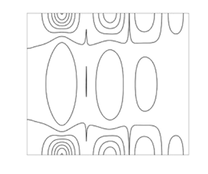
For the shoaling case, the behaviour is dramatically different. From figure 4, one can see that the cellular structure is persistent but the cells are different from each other. The variance goes through a sequence of four cells, each of which shows focusing of wave energy albeit decaying as the depth decreases. Over the first 6 km (cell I), the effect of variable depth is negligible and $\tilde {\rho }$ behaves as in constant depth; it shows a similar pattern and reaches almost the same maximum value as shown in figure 3. Over the next 5 km (cell II), one can see a second and somewhat shorter cell where the maximum of $\tilde {\rho }$ decreases to 2.8. Along the next 4 km (cell III), there is less energy concentration with a maximum of $\tilde {\rho }$ decreasing to 1.8; the energy concentration is reduced almost by half compared with the initial cell. Over the last 2 km of the domain (cell IV), there is no meaningful concentration of energy; the phenomena has disappeared and the sea state is effectively similar to a stationary wave field. Over the last cell $\mu < 0$ and, similar to the deterministic case, the instability vanishes.

Figure 4.

Long-distance evolution of the normalized variance $\tilde {\rho }$, for shoaling waters. The upper $x$-axis shows the local values of $Kh$.

In order to assess the quality of our numerical simulations, we check the conservation of the invariants, which are given in Appendix B. The first invariant is the most meaningful because it is related to the total energy. In all the examples, $I_1 = 4.18$ and it was successfully preserved by the numerical solver, with relative errors of the order of ${O}(10^{-7})$. The second invariant is always zero. The third invariant, which is only valid for constant depth, was $I_3 = 3.79$ for $h = 1000\ \textrm {m}$ and $I_3 = 3.12$ for $h = 100\ \textrm {m}$. This invariant depends both on the values along $\tau = 0$ and the values along the $\tau$-axis. The relative deviation from its value at $X = 0$ did not exceed half a percentage throughout the nonlinear computation.

6. Probability of freak-wave occurrence

The probability distribution of the wave height of a Gaussian narrow-banded wave field, is given by the Rayleigh distribution, see Holthuijsen (Reference Holthuijsen2010). Thus, at any given $(t,x)$ the probability to obtain waveheights H larger than $\hat{H}$ is:

(6.1)\begin{equation} F(\hat{H},t,x) = P(H > \hat{H}) = \exp\left[-\left(\frac{\hat{H}}{H_{rms}(t,x)}\right)^{2}\right], \end{equation}

where $H_{rms}$ denotes the root-mean-square wave height and it is related to the variance of the free-surface elevation by $H_{rms} = \sqrt {8\langle \eta ^{2}(x,t)\rangle }$, where $\langle \eta ^{2}(x,t)\rangle$ is given by (5.1).

It is useful to compare $H_{rms}$ with the root-mean-square wave height of the linear solution taken at a reference point $x_R$, so we define $H_{rms0} = \sqrt {8\langle \eta _L^{2}(x_R)\rangle }$, where $\langle \eta _L^{2}(x_R)\rangle$ is given below in (6.4), and upon normalizing $H_{rms}$, the probability of wave height exceedance at $(x,t)$ becomes

(6.2)\begin{equation} F(\hat{H},t,x) = P(H > \hat{H}) = \exp\left[-\left(\frac{\hat{H}}{H_{rms0}}\right)^{2}\frac{\langle \eta_L^{2}(x_R)\rangle}{\langle\eta^{2}(x,t)\rangle}\right]. \end{equation}

The relevant probability over a certain domain is found by averaging over such domain. Since the evolution of $\tilde {\rho }$ naturally defines different regions of interest, i.e. the recurrent cells shown in figures 2, 3 and the variable cells in figure 4, the probability of wave exceedance over each cell is given by

(6.3)\begin{equation} P(H\geq \hat{H}) = \frac{1}{(x_2 - x_1)t_{max}}\int_{0}^{t_{max}}\int_{x_1}^{x_2} F(\hat{H},t,x)\,\textrm{d}\kern0.7pt x\,\textrm{d}t. \end{equation}

Here $t_{max} = 54$ s is the period of $\tilde {\rho }$ with respect to $t$, $x_1$ is the beginning of the cell under consideration and $x_2$ is its endpoint. In the constant depth cases, the reference point $x_R = x_1 = x_0$. For the shoaling case, $x_R = (x_1 + x_2)/2$, the middle point of each of the cells.

Equation (6.3) was derived by Andrade & Stiassnie (Reference Andrade and Stiassnie2020) and was shown to be equivalent to the original equation derived by Regev et al. (Reference Regev, Agnon, Stiassnie and Gramstad2008).

Following Holthuijsen (Reference Holthuijsen2010) the significant wave height is well approximated by $H_s = 4\sqrt {\langle \eta ^{2}_L\rangle }$. The variance of the linear free surface at $x_R$ is

(6.4)\begin{equation} \langle \eta^{2}_L(x_R)\rangle = \frac{\varepsilon^{2}g^{3}}{4\varOmega^{5}\varOmega'(x_R)}. \end{equation}

The main result of this section, the probabilities of freak-wave occurrence, is given in table 1.

Table 1.

Probability of freak-wave occurrence. The values taken from the Rayleigh distribution are $0.33\times 10^{-3}$ for wave heights higher than $2H_s$, $0.15\times 10^{-7}$ for wave heights higher than $3H_s$. The columns $P/R$ are the ratios between the calculated probabilities and their corresponding values from the Rayleigh distribution.

In the cases of constant depth, due to the recurrence, only the values obtained during the first cell are shown in table 1 because they hardly differ from one cell to another. In 1000 m depth the probability of freak-wave occurrence is increased 20 times and in 100 m depth it is increased by a factor of 17 with respect to the Rayleigh distribution. By looking at extreme wave heights, higher than three times $H_s$, the probability is increased by 20 000 fold, making freak-waves encounter a feasible event.

In the case of shoaling, the results show that the probability of freak waves decreases with depth. In the deeper region, the probabilities are similar to those obtained for constant 100 m depth. From there on they decrease rapidly and towards the end of domain, in the shallower region, the probabilities are closer to the Rayleigh distribution.