


I. INTRODUCTION
Large-scale image classification is a critical task in remote sensing image processing, due to various spectral features presented in different remote sensing images. A large-scale study area is covered by several scenes of remote sensing image. Remote sensing images taken at the same time are almost impossible to collect. That means, images used for classifying large-scale study area are taken under different imaging conditions, which lead to various spectral features for the same object. Traditional methods are constructed with human-designed constraints. It is difficult for them to recognize objects imaged under different conditions.
Maximum likelihood classifier (MLC) assumes that an object of the detected image subject to a certain distribution [Reference Wei and Mendel1, Reference Sharma, Boroevich, Shigemizu, Kamatani, Kubo and Tsunoda2]. It is used as a certain method to determine land cover classes in remote sensing image classifications [Reference Keat, Abdullah, Jafri, San and Chun3, Reference Jia4]. However, it is sensitive to the changes of features in the same class. Therefore, it is also combined with feature extraction methods, such as independent component analysis, to obtain stable classification results [Reference He, Zhang, Yu and Peng5]. Nevertheless, it is barely used these years because it lacks generality. MLC cannot obtain satisfactory classification results when there exist obvious difference in imaging conditions. It is difficult to ensure the consistency of spectral features, especially for large-scale image classification.
Decision Tree (DT) is an extension of bi-classifier. It estimates the optimum thresholds to construct a stable tree structure model. Different structures of DTs may obtain different classification results. Brodley et al. [Reference Brodley, Friedl and Strahler6] demonstrated that hybrid DT outperforms univariate DT and multivariate DT for some datasets due to their ability to handle complex relationships among feature attributes and class labels. Xu et al. [Reference Xu, Yang and Liang7] proposed an improved DT by adding tree balance factor, setting node impurity and distinguishing sample types. The classification precision was improved 6.13% compared with traditional DT when performed on Longmen city of Guangdong province in China. To take advantage of geospatial knowledge, [Reference Zhang, Zhou, Huang and Zhou8] proposed a maximum variance unfolding-based co-location DT by considering the nonlinear distribution relationship of pixels in high-dimensional space. However, the selected features have a great impact on the classification results and different areas may be sensitive to different features. Besides, thresholds for the extracted features are estimated with pre-defined constraints, which also vary along with the change of image locations. Therefore, it is not suitable for classifying images covering large-scale study areas.
Random forest (RF) is an ensemble method of DTs. It overcomes the drawbacks of DT by variant DT models trained with various subsets of training samples. Therefore, it is widely used in large-scale image classification. Pelletier et al. performed RF to land cover map and obtained the following conclusions: (1) its parameter has little influence on classification accuracy; (2) adding features has little increase on the performance; and (3) the classification accuracies are affected by the landscape diversity over large area [Reference Pelletier, Valero, Inglada, Champoin and Dedieu9]. Nguyen et al. [Reference Nguyen, Joshi, Clay and Henebry10] produced a land cover map by RF used only chemometrics as input and combined the reference data augmented by cropland data layer for training and validation. By this way, the classification accuracy is significantly improved. RF is sensitive to noise and outliers due to its natural of classifying classes with a certain threshold. To solve this problem, [Reference Maas, Rottensteiner and Heipke11] proposed an adaptive RF which can take the errors in the training labels into account. By allowing a training sample to be assigned to all the classes with a certain probability, the proposed algorithm is noise tolerant.
Support vector machine (SVM) is another bi-classification model which aim to find a hyperplane with maximum margin. It uses hinge loss to calculate the empirical risk and introduces regularizations to improve the robustness of the algorithm. Xue et al. [Reference Xue, Du and Feng12] combined SVM with a break for additive seasonal and trend approach and a dynamic time warping approach to obtain land cover classification result with phenology-driven factors. Zeng and Wang [Reference Zeng and Wang13] performed the SVM classifier along with a radial basis function nonlinear transformation mapping to high-dimensional space to extract nonlinear characteristics and separability between different types. The efficiency and accuracy of the classification is significantly improved. Liu et al. [Reference Liu, Zhang, Wang and Wang14] used an adaptive mutation particle swarm optimizer to estimate the optimum parameters of SVM and employed the GKclust fuzzy clustering approach to reduce the impact of ineffective labels. Sukawattanavijit et al. [Reference Sukawattanavijit, Chen and Zhang15] combined the genetic algorithm and SVM and performed the proposed algorithm on multifrequency RADARSAT-2 and Thaichote multispectral images. Experimental results showed that the proposed algorithm outperformed the grid search approach and provided higher classification accuracy using fewer input features.
In fact, traditional image classification algorithms are constructed according to empirical constraints. They can obtain outstanding performance when the training set satisfies their constraints. Otherwise, the performance cannot meet the requirements, especially for large-scale remote sensing image classification, in which the variation of spectral features should be taken into account.
Convolutional neural networks (CNNs) have demonstrated their superiority in computer vision [Reference LeCun, Bengio and Hinton16–Reference Cheng, Yang, Yao, Guo and Han19], but its application in remote sensing image still needs to be paid more attention. There are some applications of CNNs on high resolution remote sensing images [Reference Langkvist, Kiselev, Alirezaie and Loutfi20, Reference Zhao and Du21]. However, features of large-scale Landsat images have specific difference with those of high-resolution remote sensing images, especially the texture features. Ikasari et al. demonstrates that 1-D CNNs outperform the logistic regression, SVM, and RF, and boost algorithms in Landsat image classification (which is called semantic segmentation in computer vision) and obtained an accuracy of 71.79% [Reference Ikasari, Ayumi, Fanany and Mulyono22]. Other experiments show an improvement of at least 1% of stacked autoencoder (78.99%) compared with RF, SVM, and artificial neural network (76.03%, 77.74%, and 77.86%) [Reference Li, Fu, Yu, Gong, Feng and Li23]. Similar to the field of computer vision, the pretrained model has a positive effect on remote sensing image classification. Marmanis employed pretrained model on ImageNet to fine-tune deep convolutional neural network on remote sensing images and improved the classification accuracy from 83.1% to 92.4% [Reference Marmanis, Datcu, Esch and Stilla24].
Although some CNNs have achieved great performances on Landsat images, most of them rely on patch-based training method. Patch-based training method is usually trained with fully connected CNNs. Therefore, it inputs a patch of images to the network and then the network outputs a label for the whole image. This method is based on the assumption that pixels in the patch share the same label with the central pixel. However, the assumption is not valid, especially when the central pixel locates at the boundary of a target. FCN [Reference Shelhamer, Long and Darrel25], ResNet [Reference He, Zhang, Ren and Sun26], and PSPNet [Reference Zhao, Shi, Qi, Wang and Jia27] are the most famous end-to-end networks. To obtain reliable classification results of Landsat images covering large-scale areas, we employ FCN, ResNet, and PSPNet as classifiers, and test their transfer abilities on images which did not participate in the training process.
The rest of the paper is organized as follows. Section II introduces the FCN, ResNet, and PSPNet. Section III shows the experiments of the CNNs on Landsat images. Finally, the conclusion is presented in Section IV.
II. METHODS
A) Basic modules
Assume X = {xi | i = 1, 2, …, n} is the input image, where xi = {x k | k = 1, 2, …, K} is the pixel vector of the ith pixel, k is the index of bands, K is the number of bands, i is the index of pixels, and n is the number of pixels. After the convolutional layer, the output of the lth layer is
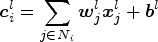
where N i is the neighborhood system of pixel i, which has the same size as the convolutional kernel, j is the index of pixels in N i, ${\boldsymbol x}_j^l$ is the pixel vector of the ith pixel in the lth layer, ${\boldsymbol w}_{j} ^l$
 is the parameters of the convolutional kernel, and ${\boldsymbol b}^l$
 is the bias.
Then the output of the lth layer is normalized to the standardized normal distribution according to the following equation:
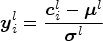
where $\boldsymbol{\mu}^l$ and $\boldsymbol{\sigma}^l$
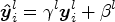
 are the mean and variance of all the pixels in the input batch, respectively. To improve the expression ability, the batch normalization (BN) layer introduces two learnable parameters and the output of BN can be expressed as:
The output of the BN layer is activated by activation function. ReLU is one of the most popular activation functions in CNN and it can be expressed as
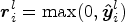
Usually, a convolutional kernel is responsible for only one possible feature. To improve the learning ability of the neural network, multi-kernels are used to extract features as much as possible. However, more convolutional kernels occupy more memory of GPU. Pooling layer is designed to overcome this problem. It can reduce the size of image while maintaining its dimension. The output of pooling layer is:
where ${\boldsymbol r}_j^l$ is the pixel in the neighbor set $N_i^l$
 which is the neighborhood system of the ith pixel in the lth layer. Actually, (5) will output the maximum value in the window of the pooling layer.
The mentioned modules are the keys to deep CNNs. Different combinations of the basic modules constitute CNNs with different structures which may be suitable for different kinds of dataset.
B) FCN
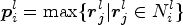
FCN is an attempt to train the network in an end-to-end way and it has achieved great success in computer vision. It replaces the fully connected layer in traditional CNNs by a convolutional layer. In FCN, the first five stacked convolutional and pooling layers in VGG-16 are used to extract features of the input image. Then the extracted feature maps are reconstructed by the upper sampling layers. In particular, to obtain reconstructed results with more detailed information, former extracted feature maps are concatenated with reconstructed feature maps. By reconstructing the feature maps layer by layer, FCN is able to maintain more detailed information. The structure of FCN is shown in Fig. 1 [Reference Shelhamer, Long and Darrel25]. First, convolutional and pooling layers are stacked to extract features of the input image. Then, the final layer (conv7) is upsampled and combined with pool4 and the combined layer is upsampled and combined with pool3 to obtain the final outputs. Compared with traditional fully connected CNNs, FCN has the following advantages:
(1) Parameters of convolutional layers are obviously less than those of the fully connected layers.
(2) The end-to-end training improves the accuracy of semantic segmentation compared with patch-based training method.
(3) There is no need for inputting images with fixed size as in traditional CNNs.
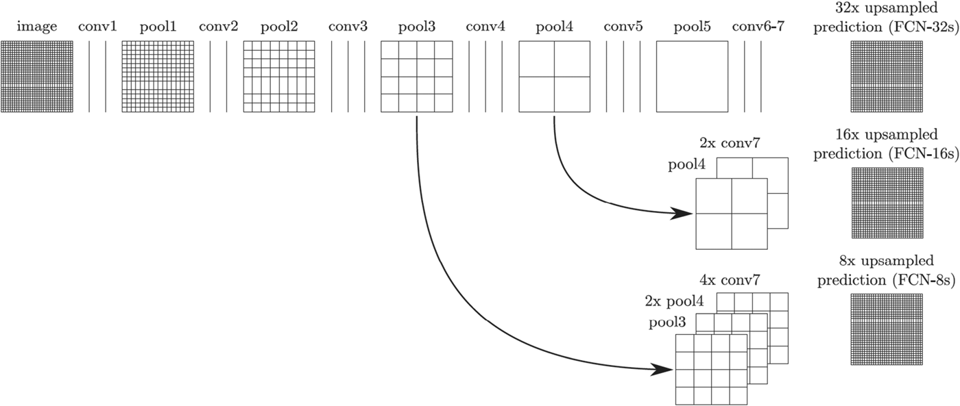
Fig. 1. Structure of FCN.
C) ResNet
Stacking convolutional layers and pooling layers to deepen the network is an efficient way to improve the learning ability of CNNs. However, increasing the depth of the network without restriction cannot improve the learning ability indefinitely. It may even result in the declination of the accuracy. Let x express the output of the former layer, it is concatenated with the later layer (after the convolution) as shown in Fig. 2 [Reference He, Zhang, Ren and Sun26].
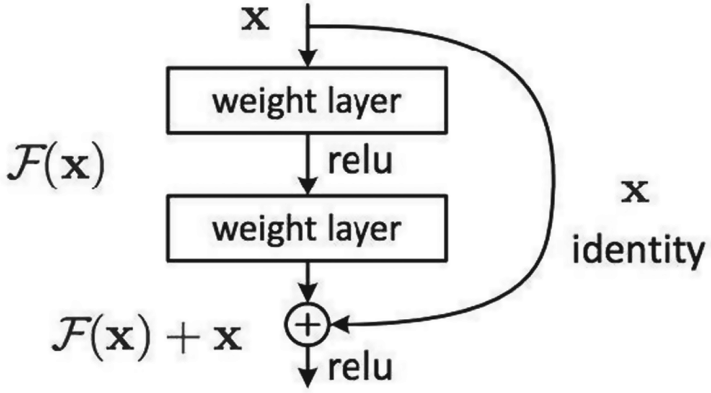
Fig. 2. Residual module.
The residual module in ResNet transmits the information of the former layer directly to the later layer. The skip connection reduces the loss of detailed information in forward propagation and allows the model to be deeper. In this paper, the fully connected layers in ResNet is replaced by convolutional layers to realize end-to-end training for Landsat image classification (also called semantic segmentation in computer vision) and we still call it ResNet for convenience.
D) PSPNet
PSPNet added a pyramid pooling layer at the end of ResNet. The connections about pyramid pooling layer is shown in Fig. 3 [Reference Zhao, Shi, Qi, Wang and Jia27]. First, the input layer (output of ResNet) is pooled into different sizes to catch information in different scales. Then the outputs of the convolutional layers with different size are unsampled to the same size of the input layer. Finally, the input layer and the outputs of pyramid pooling layers are stacked.
Fig. 3. Connections about pyramid pooling layer.
E) Flowchart
Flowchart for large-scale Landsat image classification is shown in Fig. 4. Original Landsat images are mosaicked to represent the study area. Then images of the study area are clipped to a certain size for training and inferencing convenience. The clipped Landsat images with the corresponding reference land cover map are used to train the CNN model. All clipped images covering the study area are classified by the trained model and the corresponding results are mosaicked to output the final classification results.

Fig. 4. Flowchart for large-scale Landsat image classification.
III. RESULTS AND ANALYSES
A) Performance on Jingjinji region
Jingjinji contains Beijing city, Tianjin city, and Hebei province. It is one of the most important local regions in China. The study area is covered by six first level classes, namely forest, grass land, wetland, water body, cultivated land, and artificial surface. Figure 5(a) is the false-color image of the study area composed of near infrared, red, and green bands. The original Landsat 5 images are stretched and mosaicked as shown in Fig. 5(a). The boundaries between scenes are clear due to their different imaging conditions.
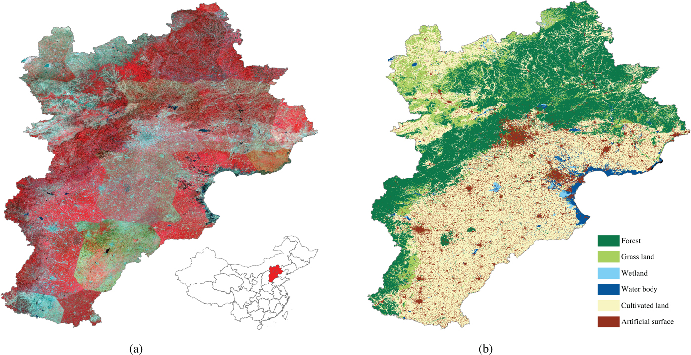
Fig. 5. Original Landsat 5 Image and reference land cover map of Jingjinji region. (a) Original image. (b) Reference land cover map.
Labels of Jingjinji area come from the “Land Cover Map of the People's Republic of China for 2010,” which can be downloaded from http://www.geodata.cn. The downloaded label map is called the reference land cover map in this paper. The original reference land cover map contains 38 second level classes with an overall accuracy of 86%. They are merged to six first level classes as shown in Fig. 5(b).
The training set is constructed by original images shown in Fig. 5(a) and reference land cover map shown in Fig. 5(b). Even though FCN, ResNet, and PSPNet can be trained in an end-to-end way, the computer cannot efficiently deal with such a large image. Therefore, the original image should be clipped for processing convenience. On the one hand, the larger the size of training sample is, the richer the local and global information it contains. On the other hand, the larger the size of training sample is, the more GPU memory is occupied. To make a trade-off between them, the size of training sample is chosen to be 512 × 512 pixels. Jingjinji region is clipped to 1600 samples with 512 × 512 pixels. These samples are used to construct two training sets. In the first training set, four-fifths are used for training and the other one-fifth is used for validation. In the second training set, we randomly select 640 images for training (about 40% of the whole samples) and another 160 images for validation. The CNN models employed in this paper are trained on 4 × Titan XP each with 12 GB memory. Although near infrared, red, and green bands are employed to show the study area, all six bands except for thermal infrared band are used to train the network. A pretrained model on ImageNet is introduced to initialize the network according to transfer learning theory [Reference Marmanis, Datcu, Esch and Stilla24].
To validate the effectiveness of FCN, ResNet, and PSPNet, we perform them on the two training sets constructed above. The training set with 80% of the training samples is called TS-1 and the training set with 40% of the training samples is called TS-2, in this paper. The classification results of FCN, ResNet, and PSPNet on TS-1 and TS-2 are shown in Fig. 6. In general, all the six classes can be distinguished in the six classification results. Classification results of FCN, ResNet, and PSPNet trained on TS-1 are more similar to the reference land cover map compared with those trained on TS-2.
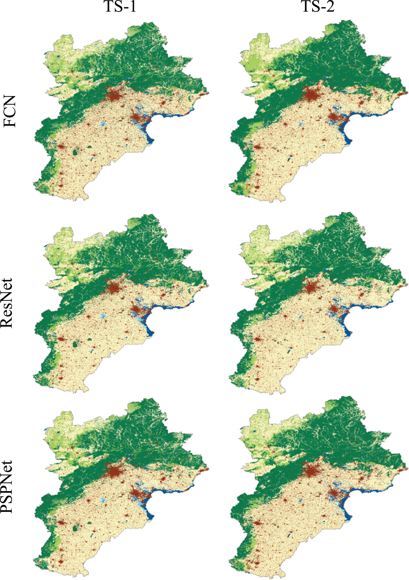
Fig. 6. Classification results of Jingjinji region from FCN, ResNet, and PSPNet with TS-1 and TS-2.
The detailed classification results of FCN, ResNet, and PSPNet on TS-1 and TS-2 are shown in Fig. 7. Figure 7(a1) is wetland. CNNs trained on TS-2 cannot recognize it very well. Actually, wetland is a disadvantage class in the training set because it only takes a small proportion in the study area. For these kinds of classes, models trained on larger training set obtains better classification results than models trained on smaller training set. Affected by imaging conditions, cultivated land in Fig. 7(b1) presents different spectral features. Accordingly, classification results in the reference land cover map (as shown in Fig. 7(b2)) classified the darker part of the cultivated land as forest. Classification results of FCN, ResNet, and PSPNet trained on TS-1 also classify this part as forest, while those obtained from TS-2 can correctly classify the darker part as cultivated land as shown in Fig. 7(b6)–(b8).
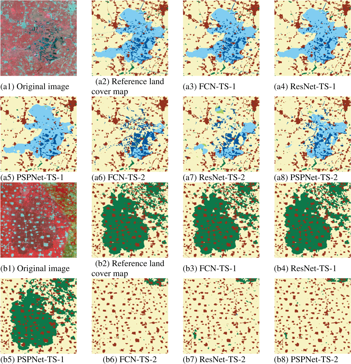
Fig. 7. Detailed Classification Results of FCN, ResNet, and PSPNet on TS-1 and TS-2. (a1) Original image. (a2) Reference land cover map. (a3) FCN-TS-1. (a4) ResNet-TS-1. (a5) PSPNet-TS-1. (a6) FCN-TS-2. (a7) ResNet-TS-2. (a8) PSPNet-TS-2. (b1) Original image. (b2) Reference land cover map. (b3) FCN-TS-1. (b4) ResNet-TS-1. (b5) PSPNet-TS-1. (b6) FCN-TS-2. (b7) ResNet-TS-2. (b8) PSPNet-TS-2.
CNNs employed in this paper are sensitive to the selection of samples. It cannot obtain satisfactory classification result when the training set contains classes which are inaccurate or insufficient. Besides, the networks tend to be overfit when trained on TS-2 with 80% of all the training samples.
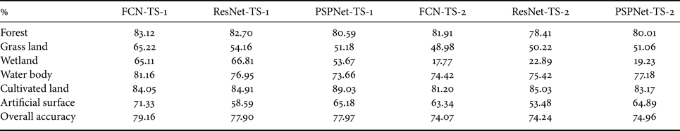
Classification accuracies of FCN, ResNet, and PSPNet trained on TS-1 and TS-2 are shown in Table 1. The accuracies of classes in classification results trained on TS-1 are all higher than those trained on TS-2. Combined with classification results shown in Figs 5 and 6, we can deduce that there are two main reasons for higher classification accuracies trained on TS-1: (1) there are enough training samples for the networks to learn detailed features of classes and (2) the classification results are overfitting. FCN obtains much higher overall accuracy (79.16%) than ResNet (77.90%) and PSPNet (77.97%) when trained on TS-1, while it obtains lower overall accuracy (74.07%) compared with ResNet (74.24%) and PSPNet (74.96%) when trained on TS-2. That means FCN is more likely to be overfit than ResNet and PSPNet. PSPNet obtains better overall accuracy than ResNet with the contribution of pyramid pooling layer. CNNs with different structures have preferences for different types of objects. For example, FCN tends to learn more detailed information of forest and artificial surface, while ResNet favors cultivated land. On the other hand, when training samples are insufficient (e.g. trained on TS-2), the learning ability of PSPNet and ResNet is slightly higher than FCN since they have much higher layers. Therefore, they obtain better accuracies on grass land, wetland, and water body with insufficient training samples. Actually, by comparing the classification accuracies of all the classes we can find that training samples has a greater impact on the classification accuracy than the structure of models.
Table 1. Classification accuracies of FCN and ResNet trained on TS-1 and TS-2.
To explore the effect of the initial learning rate, we show the changes of loss with the increase of learning rate in Fig. 8. The larger the initial learning rate is, the faster the network learns, which means the network may converge to local optimum. Smith provided a method to find the initial learning rate [Reference Smith28]. According to his method, we try the initial learning rate from 10−10 to 1 with a step of 10−1 and compare their losses. In Fig. 8, the loss is minimized when the learning rete equals to 10−4. Therefore, 10−4 is set as the initial learning rate.
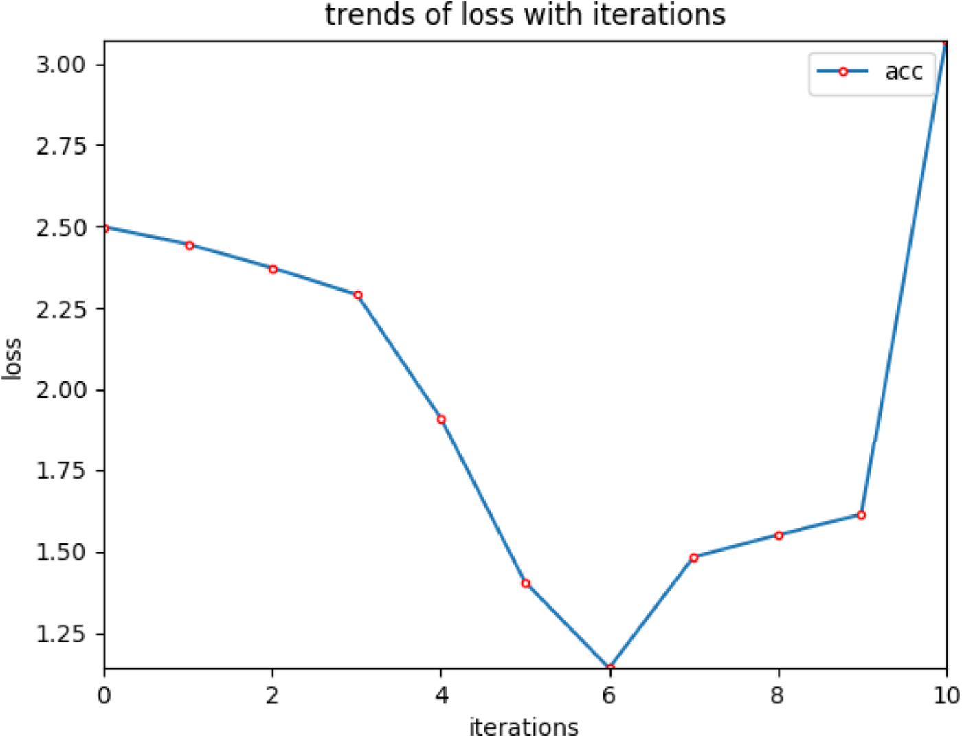
Fig. 8. Changes of loss with the learning rate.
The models are trained on 4 Titan XP GPU, each of which has 12 GB memory. FCN consumes 10 h 32 min and 6 h 24 min to train TS-1 and TS-2, respectively. Although ResNet is much deeper than FCN, it consumes less time. Its training process on TS-1 and TS-2 consume 6 h 01 min and 3 h 54 min. PSPNet consumes 7 h 21 min and 4 h 59 min to perform on TS-1 and TS-2. The reason is that, the model of ResNet and PSPNet is smaller than FCN. The parameters of the ResNet occupy 377 MB memory, PSPNet occupies 533 MB memory, while the parameters of FCN occupy 1.50 GB.
B) Transferred to Henan province
To test the generality and transferring ability of FCN, ResNet, and PSPNet, the models trained on samples of Jingjinji region are directly performed on Henan province. The original Landsat 5 images and the classification results of the trained models are shown in Fig. 9(a)–(g). In the classification results obtained by models trained on samples of Jingjinji region, there exist obvious misclassification areas as shown in the blue circles in Fig. 9(a). In these areas, artificial surface densely distributed, and the features of artificial surface have no difference compared with adjacent areas. The misclassification is caused by the special spectral features, which are obviously different with other areas. FCN tends to recognize more artificial surface compared with ResNet. Another distinct difference among the six classification results locates inside the yellow rectangle in Fig. 9(a). The six models obtain different classification results about forest, grass land, and cultivated land in this area. PSPNet trained on TS-2 tends to classify most of the cultivated land in southeast Henan province to grass land. The reason caused this phenomenon is the confusion of labels among grass lands.
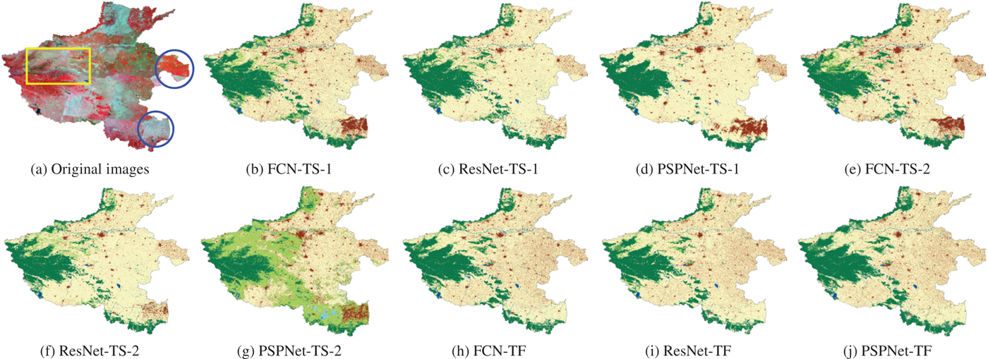
Fig. 9. Original Landsat 5 Images in Henan province and its classification results. (a) Original images. (b) FCN-TS-1. (c) ResNet-TS-1. (d) PSPNet-TS-1. (e) FCN-TS-2. (f) ResNet-TS-2. (g) PSPNet-TS-2. (h) FCN-TF. (i) ResNet-TF. (j) PSPNet-TF.
To obtain more accurate classification results in Henan province, we artificially labeled some typical training samples, and transferred the models trained on Jingjinji region to Henan province. In the transfer process, the trained model is used to initialize model parameters. Then the parameters are fine-tuned by the training set of Henan province. Performances of the transferred models are shown in Fig. 9(h)–(j). Transferred FCN, ResNet, and PSPNet are called FCN-TF, ResNet-TF, and PSPNet-TF for short.
The transferred classification results of the area in blue circlers in Fig. 9(a) are more reasonable compared with the models trained on Jingjinji region. All the CNN models can distinguish the three kinds of vegetation shown in the yellow rectangle. Besides, as the transferred models learn detailed information from the training set in Henan province, their classification results are more precise compared with models trained on Jingjinji region.
Detailed classification results of Henan province are shown in Fig. 10 to further explore the performances. Figure 10(a1) is a part in the lower blue circle in Fig. 9(a). It is covered by cultivated land but presents similar spectral features to artificial surface. Therefore, models trained on Jingjinji region cannot classify this area correctly. The transferred models are fine-tuned by the samples in Henan province. Therefore, it has a chance to learn this kind of feature of cultivated land and recognize it. Figure 10(b1) is mostly covered by cultivated land artificial surface. CNNs trained on Jingjinji region cannot distinguish artificial surface from cultivated land. While the fine-tuned models can classify this area very well. Figure 9(c1) shows another nontypical artificial surface which presents darker spectral features, while typical artificial surface has much lighter spectral features compared with the vegetation around them. Models trained on Jingjinji region cannot recognize this kind of artificial surface. On the contrary, the transferred models can obtain satisfactory classification results. The transferred models can even recognize the small water body in this area.
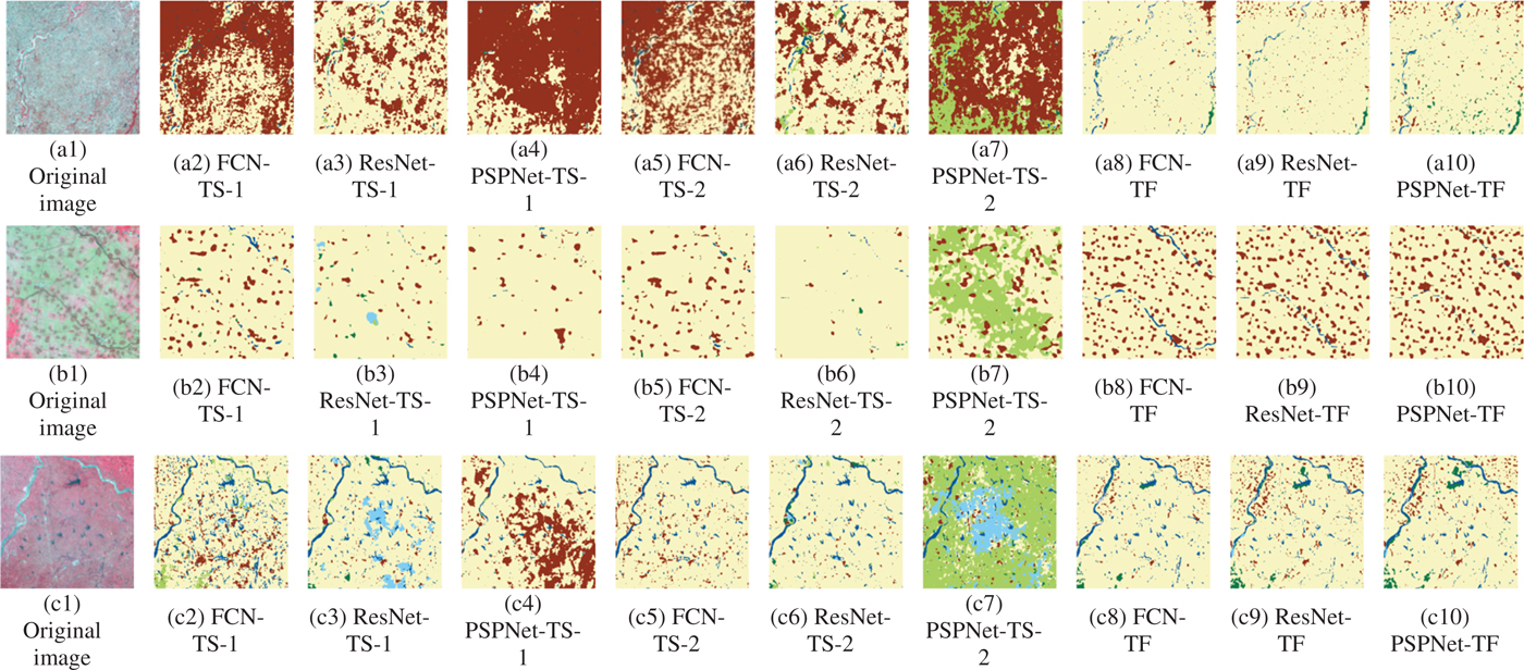
Fig. 10. Detailed classification results in Henan province. (a1) Original image. (a2) FCN-TS-1. (a3) ResNet-TS-1. (a4) PSPNet-TS-1. (a5) FCN-TS-2. (a6) ResNet-TS-2. (a7) PSPNet-TS-2. (a8) FCN-TF. (a9) ResNet-TF. (a10) PSPNet-TF. (b1) Original image. (b2) FCN-TS-1. (b3) ResNet-TS-1. (b4) PSPNet-TS-1. (b5) FCN-TS-2. (b6) ResNet-TS-2. (b7) PSPNet-TS-2. (b8) FCN-TF. (b9) ResNet-TF. (b10) PSPNet-TF. (c1) Original image. (c2) FCN-TS-1. (c3) ResNet-TS-1. (c4) PSPNet-TS-1. (c5) FCN-TS-2. (c6) ResNet-TS-2. (c7) PSPNet-TS-2. (c8) FCN-TF. (c9) ResNet-TF. (c10) PSPNet-TF.
In summary, models trained on Jingjinji region cannot recognize classes in Henan province, which have different features with those in Jingjinji region. In the models trained on Jingjinji region, models trained on TS-2 behave better than those trained on TS-1, except for PSPNet trained on TS-2. Models transferred to Henan province obtain better classification results than models directly used on Henan province. Its advantages mainly concentrate on the following two aspects: (1) stronger recognition ability and (2) finer classification results with more detailed information.
IV. CONCLUSIONS
This paper performed FCN, ResNet, and PSPNet on Jingjinji region in China with 80 and 40% of the training samples, respectively. Then the trained models are directly carried out on and also transferred to Henan province. From the experiments on Jingjinji region with different proportions of training samples, the following conclusions are drawn. (1) Inaccurate training samples may lead to overfit. (2) CNNs cannot learn detailed information from insufficient training samples. (3) Compared with ResNet and PSPNet, FCN is more likely to be overfitted. (4) CNNs with different structures have different preferences on types of objects. (5) The effect of training sample is greater than that of the structures of CNNs. Actually, performances of FCN, ResNet, and PSPNet on this study area have much similar than difference.
Classification results obtained directly from models trained on Jingjinji region and transferred from them have obviously different performances. The transferred models obtain much better classification results compared with the directly used ones. From experimental results of the models trained on TS-1, TS-2 and transferred to Henan province, we can see that: (1) CNNs cannot correctly recognize features which did not appear in the training set. (2) Classification results of insufficient models are better than overfitted ones when they are performed on images without any training samples. (3) Transferred models obtain better classification results compared with models directly carried out on target area.
ACKNOWLEDGEMENT
This research was supported by the Strategic Priority Research Program of the Chinese Academy of Sciences under Grant No. XDA19080302, the National Natural Science Foundation of China under Grant No. 41801233, and by the 62-class General Financial Grant from the China Postdoctoral Science Foundation under Grant No. 2017M620947. The authors acknowledge data support from “National Earth System Science Data Sharing Infrastructure, National Science & Technology Infrastructure of China (http://www.geodata.cn).”
Xuemei Zhao received the B.S. degree in photogrammetry and remote sensing from Liaoning Technical University, Fuxin, China, in 2012, and the Ph.D. degree in photogrammetry and remote sensing from Liaoning Technical University, Fuxin, China, in 2017. She is currently an Assistant Professor with Guilin University of Electronic Technology. Her research focuses on image segmentation and classification with deep learning and information geometry.
Lianru Gao received the B.S. degree in civil engineering from Tsinghua University, Beijing, China, in 2002, and the Ph.D. degree in cartography and geographic information system from Institute of Remote Sensing Applications, Chinese Academy of Sciences (CAS), Beijing, China, in 2007. He is currently a Professor with the Key Laboratory of Digital Earth Science, Aerospace Information Research Institute, CAS. He also has been a visiting scholar at the University of Extremadura, Cáceres, Spain, in 2014, and at the Mississippi State University (MSU), Starkville, USA, in 2016. His research focuses on models and algorithms for hyperspectral image processing, analysis and applications. In last ten years, He was the PI of 10 scientific research projects at national and ministerial levels, including projects by the National Natural Science Foundation of China (2010–2012, 2016–2019, 2018–2020), and by the Key Research Program of the CAS (2013–2015) et al. He has published more than 130 peer-reviewed papers, and there are 60 journal papers included by Science Citation Index (SCI). He was coauthor of an academic book entitled “Hyperspectral Image Classification And Target Detection”. He obtained 22 National Invention Patents and 4 Software Copyright Registrations in China. He was awarded the Outstanding Science and Technology Achievement Prize of the CAS in 2016, and was supported by the China National Science Fund for Excellent Young Scholars in 2017, and won the Second Prize of The State Scientific and Technological Progress Award in 2018. He received the recognition of the Best Reviewers of the IEEE Journal of Selected Topics in Applied Earth Observations and Remote Sensing in 2015, and the Best Reviewers of the IEEE Transactions on Geoscience and Remote Sensing in 2017.
Zhengchao Chen received the B.S. degree from Henan University of Technology, Henan, China, in 1996, the M.S. degree from Wuhan University, Wuhan, China, in 2002, and Ph.D. degree from the Institute of Remote Sensing Applications, Chinese Academy of Sciences, Beijing, China, in 2005. Currently, he is a deputy director of the Airborne Remote Sensing Center, Aerospace Information Research Institute, CAS. His research focuses on radiometric calibration of remote sensor, image processing and information extraction. In recent years, he has been working on the automatic information extraction of remote sensing images based on deep learning. He has established a remote sensing knowledge sample database with millions of samples and developed an intelligent information system with the rapid production capacity of global remote sensing data products. He has presided over more than 10 projects such as NSFC, 863, key R & D plan and leading plan of CAS, published more than 30 SCI / EI papers, and won the second prize of national science and technology progress, outstanding achievement award of CAS and first prize of science and technology progress of the whole army.
Bing Zhang received the B.S. degree in geography from Peking University, Beijing, China, the M.S. and Ph.D. degrees in remote sensing from the Institute of Remote Sensing Applications, Chinese Academy of Sciences, Beijing, China. Currently, he is a Full Professor and the Deputy Director of the Institute of Remote Sensing and Digital Earth (RADI), Chinese Academy of Sciences (CAS), where he has been leading key scientific projects in the area of hyperspectral remote sensing for more than 20 years. His research interests include the development of Mathematical and Physical models and image processing software for the analysis of hyperspectral remote sensing data in many different areas. He has developed 5 software systems in the image processing and applications. His creative achievements were rewarded 10 important prizes from Chinese government, and special government allowances of the Chinese State Council. He was awarded the National Science Foundation for Distinguished Young Scholars of China in 2013, and was awarded the 2016 Outstanding Science and Technology Achievement Prize of the Chinese Academy of Sciences, the highest level of Awards for the CAS scholars. Dr. Zhang has authored more than 300 publications, including more than 170 journal papers. He has edited 6 books/contributed book chapters on hyperspectral image processing and subsequent applications. He is currently serving as the Associate Editor for IEEE Journal of Selected Topics in Applied Earth Observations and Remote Sensing and IEEE Geoscience and Remote Sensing Letters. He has been serving as Technical Committee Member of IEEE Workshop on Hyperspectral Image and Signal Processing since 2011, and as the president of hyperspectral remote sensing committee of China National Committee of International Society for Digital Earth since 2012. He is the Student Paper Competition Committee member in IGARSS 2015, 2016 and 2017.
Wenzhi Liao received the B.Sc. degree in mathematics from Hainan Normal University, Haikou, China, in 2006, the Ph.D. degree in engineering from the South China University of Technology, Guangzhou, China, in 2012, and the Ph.D. degree in computer science engineering from Ghent University, Ghent, Belgium, in 2012. From 2012 to 2019, he has been holding a post-doctoral position at Ghent University and then a Post-Doctoral Research Fellow with the Research Foundation Flanders (FWO-Vlaanderen, Belgium). Since 2019, he has worked as a Lecturer at the University of Strathclyde. His research interests include pattern recognition, remote sensing, and image processing, and also mathematical morphology, multitask feature learning, multisensor data fusion, and hyperspectral image restoration. Dr. Liao received the Best Paper Challenge Award from the 2013 IEEE GRSS Data Fusion Contest and the 2014 IEEE GRSS Data Fusion Contest. He is serving as an Associate Editor for both the IEEE Journal of Selected Topics in Applied Earth Observations and Remote Sensing and the IET Image Processing.


 Open access