


1. Introduction
Marine terminating ice shelves found in polar regions are a vital component of Earth's climate system. The ice ablation rate, commonly called the melting rate, is determined by the magnitude of heat and solute fluxes across the ice–fluid boundary (Hewitt Reference Hewitt2020). Dynamics in the liquid phase induces convective heat and salt fluxes, leading to non-uniform melting rates in both time and space. This effect is due primarily to the introduction of turbulent fluxes and skin friction from the convection of the meltwater plume and the naturally convecting boundary layer (Jenkins Reference Jenkins2011). Accurate representations of the melting rates and their associated magnitudes are paramount in ocean and climate modelling (Alley et al. Reference Alley, Clark, Huybrechts and Joughin2005).
Marine terminating ice shelves lose mass through two main processes: direct sub-surface ablation and calving at the shelf front. Calved icebergs, in particular, represent nearly half of the freshwater flux from ice shelves into the ocean (Cenedese & Straneo Reference Cenedese and Straneo2023). Once separated from the glaciers, icebergs may drift in ocean currents and veer by storm systems and topographic steering into warmer environments where their melting rate accelerates. The eventual decay of an iceberg is driven primarily by submarine processes, including wave erosion, basal melting and buoyant vertical convection (Bigg et al. Reference Bigg, Wadley, Stevens and Johnson1997; Hester et al. Reference Hester, McConnochie, Cenedese, Couston and Vasil2021). Of these, it is generally accepted that the weakest process is buoyant vertical convection (Cenedese & Straneo Reference Cenedese and Straneo2023), which comprises both the natural convection of the ambient fluid and the resultant meltwater plume from the sides of an iceberg. In many parametrisations for iceberg decay, melting due to buoyant vertical convection is cast as a depth-averaged melting rate that has dependence only on the thermal driving  $\Delta T_a$ between the ambient fluid $T_a$ and ice–fluid interface $T_i$. The most common parametrisation is a power-law scaling (Neshyba & Josberger Reference Neshyba and Josberger1980; Josberger & Martin Reference Josberger and Martin1981; Johnson & Mollendorf Reference Johnson and Mollendorf1984; Dutton & Sharan Reference Dutton and Sharan1988; Kerr & McConnochie Reference Kerr and McConnochie2015); however, polynomial representations also appear (Neshyba & Josberger Reference Neshyba and Josberger1980; Cenedese & Straneo Reference Cenedese and Straneo2023).
One of the challenges associated with parametrising natural buoyant convection is including the influence and effects of ambient stratification. The keel depth of many icebergs can range between  $100$ and ${400}\ {\rm m}$, meaning that their penetration into the stratified water column below the mixed layer may be non-negligible (Dowdeswell & Bamber Reference Dowdeswell and Bamber2007). However, there is limited knowledge of how a stratification ultimately affects the melting rate beyond the leading-order depth-dependent driving terms (i.e. thermal or haline) and idealised predictions from plume theory (Hewitt Reference Hewitt2020).
In the laboratory experiments of McConnochie & Kerr (Reference McConnochie and Kerr2016), a vertical salinity gradient was shown to induce a depth dependency to the melting rate. Their results, albeit at conditions of weak thermal driving, highlighted that commonly used unstratified melting rate scalings become increasingly inaccurate as the natural buoyancy frequency increases. The experiments of Johnson & Mollendorf (Reference Johnson and Mollendorf1984) demonstrated further that unstratified ambient fluids with salt concentrations typical of seawater would also exhibit higher melting rates when compared to freshwater up to a thermal driving temperature approximately  ${15}\,^{\circ }{\rm C}$. A natural question for numerical models that intend to represent iceberg meltwater fluxes (e.g. Stern, Adcroft & Sergienko Reference Stern, Adcroft and Sergienko2019) is to what extent melting rates at high thermal driving depend on salt stratification in the water column. Currently, the most utilised power-law formulation posed by Neshyba & Josberger (Reference Neshyba and Josberger1980) is independent of stratification, contrary to recent evidence (McConnochie & Kerr Reference McConnochie and Kerr2016; Yang et al. Reference Yang, Howland, Liu, Verzicco and Lohse2023). Furthermore, the influence of morphological features due to the salt stratification, such as ice scalloping (e.g. Huppert & Turner Reference Huppert and Turner1980), on the average melting rate is poorly understood. Only recently, efforts with high-resolution simulations (Wilson et al. Reference Wilson, Vreugdenhil, Gayen and Hester2023; Yang et al. Reference Yang, Howland, Liu, Verzicco and Lohse2023) have begun to elucidate the complicated nature of the problem. Parametrisations that adopt the current power-law scaling are likely to perform poorly if an iceberg drifts (or is moved intentionally; Karimidastenaei et al. Reference Karimidastenaei, Klöve, Sadegh and Haghighi2021) or a glacier terminates (cf. Schild et al. Reference Schild, Renshaw, Benn, Luckman, Hawley, How, Trusel, Cottier, Pramanik and Hulton2018) into sufficiently warm waters where thermal driving is significant, stratification weakens, or knowledge of depth-wise melting is required.
Previous work on depth-dependent melting, focused primarily on unstratified environments, has determined that the key factor setting the fluxes to the ice is the dominant flow regime, laminar or turbulent, and the respective turbulent-flux regime: buoyancy-controlled or shear-controlled (Malyarenko et al. (Reference Malyarenko, Wells, Langhorne, Robinson, Williams and Nicholls2020) and references therein). Ultimately, heat and solute fluxes from the fluid are transferred via diffusion to the ice through a thin molecular boundary layer of thickness  $\delta$, where the fluxes are inversely proportional to $\delta$. Considering only vertical ice faces, laminar convection predicts that $\delta$ will grow monotonically per unit distance alongslope until convective instability occurs and is followed by turbulent convection. After the transition to turbulence, $\delta$ is suppressed and modulated through eddy kinetic energy and shearing forces generated in an outer turbulent boundary layer, depending on the dominant turbulent-flux regime (Wells & Worster Reference Wells and Worster2008). The buoyancy-controlled regime is typically attributed to naturally convecting systems where buoyancy provides a mechanism for turbulent production, with $\delta$ scaling with the global Rayleigh number and the fluxes scaling with the third root of the flow buoyancy, $b^{1/3}$. The shear-controlled regime is assumed to be produced from externally forced flows (e.g. tides) or when a buoyant convection flow transitions to shear-controlled if a critical Rayleigh number is exceeded (Kerr & McConnochie Reference Kerr and McConnochie2015), with $\delta$ scaling with the Reynolds number, and the fluxes scaling with the free-stream flow speed. The corollary of these flux regimes is that the local melting rate is also controlled through local buoyancy and free-stream flow speed. For melting ice in unstratified fluids, solutions to the turbulent-flux regimes through self-similar turbulent theory predict a depth-dependent power-law profile, where melting increases with distance from the flow origin (Josberger Reference Josberger1979). However, in the more geophysically relevant case of melting into stratified fluids, the depth-dependent solutions are non-trivial and must be solved numerically (e.g. Magorrian & Wells Reference Magorrian and Wells2016).
In certain salt-stratification conditions, the formation of thermohaline staircases and circulation cells via double-diffusive convection has been shown to play a role in regulating melting rates (Stephenson et al. Reference Stephenson, Sprintall, Gille, Vernet, Helly and Kaufmann2011; Rosevear, Gayen & Galton-Fenzi Reference Rosevear, Gayen and Galton-Fenzi2021; Wilson et al. Reference Wilson, Vreugdenhil, Gayen and Hester2023). The seminal laboratory study by Huppert & Turner (Reference Huppert and Turner1980) (HT80) demonstrated that for vertical ice melting into a salinity gradient, thermohaline staircases (hereafter, layers) form with thicknesses proportional to the depth-averaged density difference between the ambient fluid and its respective isohaline freezing density, and inversely proportional to the ambient fluid's density gradient. The presence of these layers was shown to characterise the spatial structure of the melting rates as the ice face became arranged into a scalloping pattern, with the troughs (peaks) of each scallop coinciding with the core (boundary) of a layer. Although the exact melting rates within each layer were not reported, the scalloping patterns were of a profile that suggests a flow-dependent melting rate, where buoyancy is gained through fluxes to the ice, and lost through vertical displacement in a salt stratification (cf. Baines Reference Baines2002). Similar scalloping patterns of ice have also been shown to manifest from flow-dependent processes unrelated to double-diffusion. Small-scale scallops (1–20 cm), common to many icebergs and ice shelves, have been observed to be created by trapped eddies generated from forced convection flows (Josberger & Martin Reference Josberger and Martin1981; Bushuk et al. Reference Bushuk, Holland, Stanton, Stern and Gray2019) and also by a density reversal (Weady et al. Reference Weady, Tong, Zidovska and Ristroph2022). While the forcing mechanism differs, in both cases, the circulation structure in the ambient fluid regulates the heat, salt and volume fluxes to the ice, and therefore controls the local melting rate.
The studies cited above raise the critical question of what flux scaling law best describes the melting rate in stratified environments with active double-diffusive convection. Here, we explore this question by investigating the influence of (relatively weak) salt stratification on the local and depth-averaged melting rates through a series of laboratory experiments at conditions of high thermal driving ( $\Delta T_a>{10}\ {\rm K}$) with initially uniform far-field temperatures, a regime that previously has not been investigated experimentally (McCutchan & Johnson Reference McCutchan and Johnson2022). In § 2, we outline the experimental set-up and data collection methodology. We describe our results and evaluate the validity of existing parametrisations in § 3. A discussion of the results follows in § 4, and we conclude in § 5.
2. Methods
2.1. Apparatus and set-up
The apparatus shown in figure 1(a) consisted of a tank constructed out of double-glazed Perspex and reinforced with steel square beams, measuring  ${1.5}\ {\rm {m}}\times 1.1\ {\rm m}\times 0.2\ {\rm m}$ ( $\hat {x}$, $\hat {z}$ and $\hat {y}$ directions, respectively) housed in a constant-temperature room within the Climate and Fluid Physics laboratory at the Australian National University (cf. Kerr & McConnochie Reference Kerr and McConnochie2015). The double-glazed panes were filled with argon gas to reduce the moisture content and prevent condensation. The tank width ( ${0.2}\ {\rm m}$) is sufficient to accommodate three-dimensional turbulence at small scales and the expected large-scale two-dimensional double-diffusive convection cells and ice morphology (cf. Yang et al. Reference Yang, Howland, Liu, Verzicco and Lohse2023), as well as meaning that viscous boundary effects and any sidewall heat fluxes may be neglected safely. Within the tank, a ${1.5}\ {\rm m}\times 0.2\ {\rm m}$ ( $\hat {z}$ and $\hat {y}$) heat exchanger plate connected to a Julabo FP50-HD refrigerated circulator was placed along one of the sidewalls and used to grow and sustain a slab of ice at temperatures $T_s\approx -20\,{^\circ }{\rm C}$.
Schematic of the experimental set-up: (a) the experiment tank and its components in an observer reference frame at the initiation time of an experiment (ice-shape is rounded for added emphasis); (b) top-down view; and (c) modified ‘double-bucket’ system (not to scale). The coordinates  $(x,z,y)$ denote the positive horizontal, vertical and lateral directions for length, depth and width. Tank measurements $(L,H,W)$ represent spanwise length, height and width, respectively. Temperatures $T$, salinities $S$ and densities $\rho$ are indexed by their respective feature: $s,i,a$ for solid, interface and ambient, respectively. Ice thickness $h(z,t)$ is measured normal to the sidewall at $x={0}\ {\rm m}$, beginning with an initial thickness $h_0(z)$.

Creation of a salt-stratified fluid in the tank was accomplished by pumping mixed fluid into the base of the tank through the use of a modified ‘double-bucket’ arrangement composed of two 200 l drums, constant head pressure outlets, a SmartMotor-controlled mixing valve, and a pump (figure 1c). Usage of the modified double-bucket technique was necessary as overhead space was limited, meaning that a gravity-fed injection was not feasible. The constant pressure heads and pump maintain a constant flow rate, while the mixing valve ensures the correct ratio of ‘salty’ and ‘fresh’ throughout the fill via a Labview control program. For each experiment, the drums were preheated to the desired ambient temperature  $T_a$, and preset with the desired salt concentration to fix the upper ( $\rho _{min}$) and lower bounds ( $\rho _{max}$) of the stratified fluid (refer to figure 1a). A viewing area spanning the full depth of the tank and $0.25\ {\rm m}$ in width was covered with shadowgraph paper and illuminated with white light by a projector located ${5}\ {\rm m}$ behind the tank (virtual distance). Images of this area were taken on a high-speed/resolution Basler camera positioned ${3}\ {\rm m}$ in front of the tank (figure 1b) operating at variable time intervals ${500}\ {\rm ms}$ (for a duration up to ${1}\ {\rm h}$) and ${1}\ {\rm min}$ with a calibrated spatial resolution of approximately ${0.3}\ {\rm mm}$.
Experiments were carried out by initially growing pure ice in the tank from freshwater (air bubbles in the ice were prevented by using an air stone to drive a continuous flow along the ice surface during solidification) until the  $x$-wise initial thickness of the ice was $h_0\approx {0.15}\ {\rm m}$ (10 % of experiment tank thickness). As the ice is grown in situ, the horizontal temperature profile within the ice is expected to span the prescribed temperature $T_s$ at the heat exchanger and the interface temperature $T_i$ prescribed by the equilibrium condition at the ice–fluid interface (i.e. the liquidus curve) through a constant temperature gradient. As such, colder heat exchanger temperatures imply that more sensible heat must be delivered to the ice to heat up and melt the ice, but this is a relatively modest effect. Using the Stefan number ${\textit {St}}=c_s(T_i-T_s)/\mathcal {L}$, where $c_s\approx 2000\ {\rm J}\ {\rm kg}^{-1}\ {\rm K}^{{-1}}$ is the specific heat capacity of ice, and $\mathcal {L}=3.35\times 10^{5}\ {\rm J}\ {\rm kg}^{{-1}}$ is the latent heat of fusion, we estimate that our configuration (with $T_s=-20\,^{\circ }{\rm C}$) requires approximately an extra 11 % of energy for the same melting rate as compared to previous studies where $T_s\approx -1\,^{\circ }{\rm C}$ (refer to McCutchan & Johnson Reference McCutchan and Johnson2022). The room temperature was then adjusted to match $T_a$, and the ice was partitioned off from the freshwater within the tank with a removable barrier slotted flush with the ice face. The remaining freshwater was then preheated to $T_a$ followed by the injection of the salt-stratified fluid from the bottom of the tank, with the freshwater overflowing (to the drain) out the top. Typical injection durations were approximately 1.5 h, and due to the temperature differential, some premature melting was observed due to conduction through the barrier during this time. On average, premature melting resulted in a change in $h_0$ between ${1}\ {\rm mm}$ (coldest) and ${10}\ {\rm mm}$ (warmest) experiments; this premature melting is not included in our reported results. Upon creating the desired salt-stratified environment, the barrier was removed carefully ( $\approx$2 min) to minimise disturbance to the stratification, and the system's evolution was recorded for up to ${12}\ {\rm h}$. We note that a short-lived disturbance to the entire fluid was generated during the removal of the barrier, resulting in a barotropic sloshing motion that would persist for approximately ${5}\ {\rm min}$. We also report that throughout the course of an experiment, regardless of the room temperature, there was no evidence of significant sidewall melting.
In other reference experiments with a non-salt-stratified fluid, a procedure similar to that described above was followed except for the double-bucket technique, which was replaced by direct replenishment of fluid at  $T_a$ into the experiment tank. To maintain a homogeneous ambient temperature profile and prevent the pooling of densified ambient fluid at the bottom of the tank, ultimately causing the development of a strong thermal stratification, a diffusing screen and a mixing reservoir similar to that detailed in Josberger & Martin (Reference Josberger and Martin1981) were implemented. Further details of this unstratified configuration are given in § A.2.
2.2. Measurements: stratification, thermal driving, and ice melting rate
Measurements of the ambient fluid density were taken with a DMA-15 densimeter during (automated via an in-line connection) and immediately after injection into the tank (via sampling tubes), with density profiles found to be linear before removal of the barrier. The salinity profile in each experiment was inferred from the measured density profile through a realistic equation of state (Roquet et al. Reference Roquet, Madec, Brodeau and Nycander2015). We define the initial buoyancy frequency as
 \begin{equation} N^2=\frac{g}{\rho_0}\,\frac{\partial \rho_a}{\partial z}, \end{equation}
where the reference density is  $\rho _0=999.8\ {\rm kg}\ {\rm m}^{{-3}}$, and $g$ is the acceleration due to gravity. The buoyancy frequency was calculated from a linear regression of the measured density gradient. Except for the non-salt-stratified cases, $N$ is assumed to be characterised by the salinity gradient. Thermal driving is defined as $\Delta T_a=T_{a}-T_{i}$, where $T_{a}$ is the initial ambient temperature (assumed constant throughout the tank), and $T_{i}$ is the mean interface temperature, which may be approximated as the liquidus temperature $T_L$ for an isohaline transformation of the ambient fluid (Vancoppenolle et al. Reference Vancoppenolle, Madec, Thomas and McDougall2019):
 \begin{equation} T_i=T_L(\bar{S}_a). \end{equation}
For all our experiments,  $T_i\gtrapprox -0.54\,^{\circ }{\rm C}$, but hereafter we will assume $T_i={0}\,^{\circ }{\rm C}$ in the interests of brevity. Small variations in $T_i$ due to salt concentrations are unimportant in the high-temperature regimes of these experiments, and an uncertainty of $\pm {1}\,^{\circ }{\rm C}$ is assumed for $T_a$ in all experiments, which is the variability in the room temperature control. We note that since our apparatus does not have an opposing heat exchanger to maintain the constant temperature in the ambient fluid, there is an inherent time limit to each experiment owing to the finite size of the tank before $T_a$ changes appreciably. An estimate for this time ( $\tau _0$) can be sourced from the lateral growth rate of the layers (Malki-Epshtein, Phillips & Huppert Reference Malki-Epshtein, Phillips and Huppert2004) and is considered when calculating the average melting rate.
Measurements of ice thickness were obtained by analysis of the shadowgraph images. The morphological changes to the ice–fluid interface were tracked spatiotemporally through a pipeline of filtering and edge-detection techniques (Kerr & McConnochie Reference Kerr and McConnochie2015), with the ice thickness relative to the sidewall denoted by  $h(z,t)$. Applying this algorithm to the time series of images and taking the time derivative returned measurements of the instantaneous melting rate ${m}(z,t)=-\partial h(z,t)/\partial t$.
2.3. Measurements: fluid velocity and boundary layer
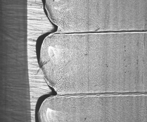
The fluid's time-averaged horizontal and vertical velocity components were measured by tracking flow features in the captured shadowgraph images (figure 2). Such measurements were made possible due to light intensity  $I(x,z,t)$ variations arising from curvature in fluid densities ( $\nabla ^2\rho$) inducing optical caustics on the shadowgraph. To improve the measurement and fidelity of the flow speeds, especially at conditions of lower thermal driving, image time series were converted into transient light intensity fields by subtracting a rolling time mean (background) field of 5 image frames before analysis (figures 2a,b). Since fluxes to the ice are moderated through the boundary layer, particularly via shear stresses, we focus on measuring its flow speed. The boundary layer is assumed to be composed of a wall-bounded meltwater plume of thickness $\delta _m$ adjacent to the ice, and an ambient fluid plume component outside of it, extending into the far field of thickness $\delta _a$ (cf. Yang et al. Reference Yang, Howland, Liu, Verzicco and Lohse2023) where the horizontal velocity is zero at the interface and the outer edge of the ambient layer (Carey & Gebhart Reference Carey and Gebhart1982; Wells & Worster Reference Wells and Worster2011). Because the meltwater component has the potential to be positively or negatively buoyant with respect to the ambient component (discussed in § 2.4) and the salt stratification could also affect the flow, the horizontal profile of the boundary layer is not easily generalisable since it is not necessarily constant throughout the entire fluid column. As such, we have simplified the task by considering only the maximum vertical velocity of the horizontal profile throughout the fluid column as the characteristic boundary layer flow speed (figure 2c).
A close-up image of the ice–fluid interface ( $T_a=30\,^{\circ }{\rm C}$). (a) The shadowgraph image, as captured by the camera. Some residual dye in the fluid can be seen at upper right. (b) The transient light field (a proxy for $\nabla ^2\rho$), extracted from a subtraction of the shadowgraph image (a) and a rolling time average. This field's various features (e.g. filaments and turbulence) were used to measure fluid velocities. (c) False-colour composite of two transient images in the time series ( $\Delta t\approx 500\ {\rm ms}$, blue–red colour denotes a feature change between images) with examples of the horizontal boundary layer velocity $U(x)$, our definition of the vertical flow speed $U(z)$, a filament being tracked, and its error window $\sigma _U$.

We further restrict the region of interest to be between the ice–fluid interface and the maximum effective width of the plume, approximately  ${4}\ {\rm cm}$ into the fluid (in the $\hat {x}$ direction). Optical features (see figure 2b) were tracked within this region until either substantial dissipation of the feature or significant departure from the region occurred. Outside this region, the flow is assumed to not contribute to the fluxes needed for melting. This procedure was carried out over many sequences of images spanning the available time series to develop a complete picture of the boundary layer flow speed over time and depth. Instantaneous uncertainties were defined by an error window $\sigma _U$ about each measurement based on probable flow trajectories inferred from neighbouring flow features, representative of both the systematic (e.g. chaotic motion) and random (e.g. feature distortions) error (see figure 2c). In addition, we used an Optical Flow package (Liu & Salazar Reference Liu and Salazar2021) to assist in identifying the unidirectional and bidirectional flow regimes as well as provide a qualitative view of the flow field (discussed in § A.3). We restricted the implementation of this technique to these insights chiefly due to inconsistencies in the calculated velocity magnitudes that occurred in the presence of vigorous turbulence.
2.4. Parameter space and expected flow dynamics
A total of 11 experiments were conducted, two of which were non-salt-stratified, at five different temperatures spanning  ${10}\,^{\circ }{\rm C}$ to ${30}\,^{\circ }{\rm C}$ (see table 1). We emphasise that our parameter space is notably different from that found in the ocean, especially in density space where the ambient fluid density is comparable to that of meltwater, significantly influencing the dynamics that we observe. The meltwater from pure ice may be assumed to be ejected at close to the reference density in conditions of high thermal driving, and has buoyancy $b_m\propto \rho _a-\rho _0$. By contrast, the ambient fluid plume is always expected to cool and gain a buoyancy $b_a\propto \rho _a-\rho (S_a,T_i)$ that, given the appropriate temperature and salinity conditions, downwells when the thermal expansion coefficient $\alpha (S,T)$ is positive. Comparing the relative contributions of each plume when $\alpha >0$ indicates that $b_m/b_a<0$ results in a downwelling unidirectional flow, whereas $b_m/b_a>0$ results in bidirectional flow with meltwater upwelling. For our parameter space, this implies that meltwater can change between upwelling ( $\rho _0<\rho _a$) or downwelling ( $\rho _0>\rho _a$) depending on the temperature and salinity of the ambient fluid, and because the salinity field is also a function of depth, also exhibit both flow states throughout the fluid column. These facts mean ultimately that various flow regimes in the boundary layer spanning the unidirectional upwelling and downwelling cases are possible, depending on the ambient conditions. For unstratified environments, the mapping for the resultant boundary layers is known from Carey & Gebhart (Reference Carey and Gebhart1982). Based on their work, we generally expect the dominant contributor of the boundary layer flow to transition from a bidirectional but mostly upwelling meltwater plume at cold temperatures, to a mostly downwelling ambient fluid plume at $T_a\approx 20\,^{\circ }{\rm C}$ as the ambient temperature is increased. However, we also anticipate the salt stratification impeding the flow regimes and being influenced by double-diffusive convection as described by HT80. We note for clarity that the unidirectional downwelling dynamics are not representative of typical ocean salinities ( ${\approx }35\,\unicode{x2030}$), as meltwater is significantly more buoyant relative to the ambient fluid and will generally dominate the boundary layer flow.
List of experimental parameters for the primary set of five salt-stratified experiments and key results. Uncertainty for  $N$ is $\pm {0.001}\ {\rm rad}\ {\rm s}^{{-1}}$. Observed initial cross-sectional area of ice $A_0$, characteristic melting times $\tau$, depth-averaged melting rates $\bar {m}$, depth-averaged stratification length scales $\bar {\eta }$ following HT80 and observed depth-averaged layer thickness $\bar {\eta }$ and their ratio, as well as the number of layers. The thermal Rayleigh number evaluated at the stratification length scale ${\textit {Ra}}_{\bar {\eta }}$ (3.2) using observed values and the global thermal Rayleigh number ${\textit {Ra}}_H$, depth-averaged Nusselt number $\overline {{\textit {Nu}}}_H$ (3.8), and depth-averaged boundary layer flow speed $\bar {U}$. Variables enclosed by angled brackets denote time-averaged values across $0\leq t\leq {\tau }$.

3. Results
Here, we focus on a primary set of five experiments with similar salt stratifications and reference salinities of approximately  $0\,\unicode{x2030}$, but with varying thermal driving. Additional experiments with different salt and thermal stratification and reference salinities are described in § A.1. Uncertainties in the results that follow are all given at one standard deviation. We begin with a synopsis of the characteristic ice melting behaviour and overall flow dynamics, followed by quantitative analyses of the layering, melting rates and boundary layer flow speed.
3.1. Qualitative observations
In all experiments, ice was observed to melt from a planar state of near-constant thickness  $h_0$ and rapidly morph into distinct ice scallops. Figure 3(a) shows example snapshots of the ice face from each experiment at a time when scallops are well established. The morphological evolution of the ice face, as shown in figure 3(b) in terms of the ratio of ice melted, demonstrates that once formed, scallop positions and peak-to-peak distances (hereafter, scallop wavelength) are mostly constant for the duration of the experiment. As inferred from the consistent shape of ice thickness contours in figure 3(b), the scallop wavelengths appear to be near constant within each case, but growing as a function of thermal driving. This observation is generally consistent with the ice scallops observed by HT80, with scallop wavelengths appearing to follow the characteristic stratification length scale scaling $\bar {\eta }$ predicted therein (see § 3.2). However, as $T_a$ increases, the scallop profiles observed in our experiments change between experiments from symmetrically concave shapes to asymmetrical sawtooth-like shapes (the sawtooth shape is exemplified in figure 3b iv). We note that this kind of scalloping is dissimilar to that reported in Bushuk et al. (Reference Bushuk, Holland, Stanton, Stern and Gray2019) and Weady et al. (Reference Weady, Tong, Zidovska and Ristroph2022), which has wavelengths on the $O({5}\ {\rm cm})$ scale and manifests from self-reinforcing eddies trapped between the boundary layer flow and ice–fluid interface, but is broadly consistent with the observations of Yang et al. (Reference Yang, Howland, Liu, Verzicco and Lohse2023). The lack of smaller-scale scalloping features in our experiments suggests that the flow dynamics influenced by the density extremum (cf. Weady et al. Reference Weady, Tong, Zidovska and Ristroph2022) are irrelevant in the present experiments. We remark that no evidence for significant spanwise variations in the melting of ice, as well as small-scale three-dimensional turbulent melting (e.g. Josberger Reference Josberger1979), was observed in our experiments, and as such, we maintain that any sidewall fluxes and boundary effects can be negated from our upcoming analyses.
An array of experimental data for experiments with different  $T_a$. (a) Characteristic snapshots of the ice (greyscale value $I(x,z)$) at times of proportionally equally melt $t\approx 2\tau$ (refer to table 1), where $\tau$ demarcates the time when $1/{\rm e}$ of the total fraction of ice has melted. (b) Fraction of ice melted in time, where $h(z,t)$ denotes the thickness of ice with respect to its initial thickness $h_0$. Contours denote one-tenth of a multiple of $\tau$. (c) Transient light-field intensity anomalies (proxy for $\nabla ^2\rho$) near $x\approx 0.2\ {\rm m}$, useful in the identification of fluid-layer interfaces (solid, markings, $t=\tau$) and plume detrainment (dotted, cyan lines). Columns are ordered by $T_a$ as given in (a).

We find that the formation of ice scallops occurs in conjunction with the development of a ‘thermohaline staircase’ like fluid layers and associated internal circulation cells. The distinct banded lines in figure 3(c) show the strong density interface at the boundaries of these layers, as measured in the observable far field away from the ice face ( ${\approx }0.2\ {\rm m}$). These internal circulation cells (represented by red arrows in figure 3a) grow rapidly to the full thickness of each layer and eventually span the length of the tank, as observed over time. We observe a small degree of spatial variability in the depth of the layer interfaces, including merging and splitting events (cf. Radko et al. Reference Radko, Flanagan, Stellmach and Timmermans2014) as well as an initial uplift towards the free surface. The merging and splitting events are a stochastic stabilising mechanism inherent to all thermohaline structures (Radko et al. Reference Radko, Flanagan, Stellmach and Timmermans2014), and the initial uplift behaviour is likely due to the sudden deposition of meltwater into the ambient fluid. In addition to the well-defined density layers, when $T_a>20\,^{\circ }{\rm C}$ additional fluid layers that exhibit a much weaker density interface are also observed. These weak-density interfaces, which shift linearly towards the free surface with time, are identified to be detraining outflows from a ‘peeling plume’ (cf. Bonnebaigt, Caulfield & Linden Reference Bonnebaigt, Caulfield and Linden2018). These detraining outflows (see figures 3a iv–v) do not appear to affect the melting rate in their local vicinity directly.
Boundary layer flows, both upwelling and downwelling, made evident through the transient light field, were observed in all cases. The relative strength of the boundary layer flow speed was observed to increase with the magnitude of thermal driving. Experiments at lower temperatures ( $T_a<20\,^{\circ }{\rm C}$) exhibited a mix of laminar and weakly turbulent downwelling flow in addition to a turbulent upwelling meltwater component, typically between the ice face and the downwelling flow, that was able to penetrate multiple layer interfaces, as illustrated in figures 3(a i–ii) (cyan arrows). Experiments with $T_a\geq 20\,^{\circ }{\rm C}$ demonstrated a distinctive turbulent boundary layer flow downwelling at the ice–fluid interface, intruding horizontally at either the bottom of the tank or a layer interface (e.g. figure 3a iii). For these cases, where multiple layers were present, an immediate transition to turbulence was observed at the ice–fluid interface below the first layer. This behaviour is a result of double-diffusive fluxes across the layer interface, where cold freshwater sits above a warm salty layer, which produces a thermohaline instability (Huppert & Turner Reference Huppert and Turner1980; Radko et al. Reference Radko, Flanagan, Stellmach and Timmermans2014). Additionally, the effective thickness of the boundary layer flow ( $\delta _m+\delta _a$), which we determined as the point of a sudden decrease in discernible fluid motion in the boundary layer flow away from the ice–fluid interface, was observed to grow with increasing thermal driving. Typical thicknesses were $O(0.5\ {\rm cm})$ in the coldest case ( $T_a={10}\,^{\circ }{\rm C}$), and $O({4}\ {\rm cm})$ in the warmest case ( $T_a={30}\,^{\circ }{\rm C}$). We also note that downwelling laminar flows were observed in all cases near the free surface (figure 3a, orange arrows), transitioning to turbulence after approximately $10\unicode{x2013}{20}\ {\rm cm}$ alongslope, or at the first layer interface (case-dependent).
3.2. Layers
Measurements of the fluid layer thicknesses were made by examining the scallop wavelengths and proxy field for curvature in fluid density, as shown in figures 3(a) and 3(c), respectively. The stratification length scale is defined as
 \begin{equation} \bar{\eta}=\mathcal{H}\,{\Delta\bar{\rho}}\left|\frac{\partial\rho_a}{\partial z}\right|^{-1}, \end{equation}
where  $\mathcal {H}=(0.66\pm 0.06)$ is an empirically determined scaling coefficient, $\Delta \bar {\rho }$ denotes the depth-averaged density difference between the ambient water $\rho _a$ and its respective isohaline freezing point density, and $z$ is the vertical coordinate (HT80). Table 1 summarises the number of layers, their depth-averaged thicknesses compared to the stratification length scale (3.1), and thermal Rayleigh number
 \begin{equation} {\textit{Ra}}_{Z}=\frac{g\alpha\,\Delta T_a\,Z^3}{\nu\kappa_T}, \end{equation}
where  $Z$ is a characteristic vertical length scale, $\alpha$ is the thermal expansion coefficient, $\nu$ is the dynamic viscosity, and $\kappa _T$ is the thermal diffusivity of water, for each of the experiments shown in table 1. We note that all coefficients in (3.2) are evaluated at their respective $T_a$ and $\bar {S}_a$ values. The tabulated results demonstrate that the layer thicknesses are consistent within uncertainty with the theoretical scaling of HT80, albeit with somewhat larger uncertainty at lower ambient temperatures. The empirical scaling coefficient for $\bar {\eta }$ reported by HT80 has known validity in $10^5\lessapprox {\textit {Ra}}_{\bar {\eta }}\lessapprox 10^9$ and for $\bar {\eta }\approx O({50}\ {\rm mm})$, and is stated to exhibit no systematic dependence on the Rayleigh number beyond the critical value ${\textit {Ra}}_{\bar {\eta }}\approx 10^5$ necessary for the development of the layers. To our knowledge, our experiment is the first to investigate vertical ice melting into a salt-stratified fluid with stratification length scales exceeding ${0.2}\ {\rm m}$ and ${\textit {Ra}}_{\bar {\eta }}>10^9$, a value slightly beyond the critical transition point to turbulent-free convection (Wells & Worster Reference Wells and Worster2008). From our data, it appears that the empirical scaling coefficient remains valid following the onset of turbulent-free convection up to ${\textit {Ra}}_{\bar {\eta }}\approx 10^{11}$. Notably, this value and its global counterpart ${\textit {Ra}}_H$ (refer to table 1) are still much less than the critical value $10^{21}$ for a shear-controlled flux regime (Kerr & McConnochie Reference Kerr and McConnochie2015).
3.3. Depth-averaged melting rate and steady melting rate assumption
The depth-integrated melting rate of ice through the entire fluid column is examined using the fraction of ice melted,  $\phi$, hereafter termed the melt fraction, defined by
 \begin{equation} \phi(t)=1-\frac{\displaystyle\int_0^H h(z,t)\,{\rm d}z}{A_0}, \end{equation}
where  $A_0$ is the initial cross-sectional area of ice,
 \begin{equation} A_0=\int_0^Hh_0(z)\,{\rm d}z. \end{equation}
It then follows that the depth-averaged melting rate is defined through
 \begin{equation} \bar{m}=\frac{1}{H}\int_0^H m(z,t)\,{\rm d}z=\frac{A_0}{H}\,\frac{\partial \phi(t)}{\partial t}. \end{equation}
Figure 4 showcases how the melt fraction is implemented to calculate the depth-averaged melting rate in a state of non-acceleration. We define a characteristic time  $\tau$ such that $\phi (\tau )=1/{\rm e}$; that is, $\tau$ is the ${\rm e}$-folding time scale for ice melting (see values in table 1). As shown in figure 4(a), the melt fractions for each experiment exhibit similar temporal evolution, with two distinct phases before and after $t\approx \tau$. The first phase is a period of constant melting rate, up to a time $\tau$ (which reduces with increasing $T_a$). The second phase involves a gradual reduction in melting rate as the ambient fluid approaches thermal equilibrium and a greater fraction of the heat supplied to the ice must be used for sensible heating rather than melting. We find that this time scale definition is comparable to the inherent time limit $\tau _0$ for an unmaintained ambient fluid temperature field (Malki-Epshtein et al. Reference Malki-Epshtein, Phillips and Huppert2004), which indicates that melting for $0\leq t\leq \tau$ is representative of a constant $T_a$. We note that the sudden approach of $\phi$ towards unity for $T_a={25}\,^{\circ }{\rm C}$ near $t={4}\ {\rm h}$ is due to the calving of the uppermost section of ice from the heat exchanger (cf. figure 3b iv). In the following analysis, we focus on the initial non-accelerating melting rate phase.
Depth-integrated melting rates: (a) net melted-ice fraction  $\phi (t)$; (b) net melted-ice cross-section with non-accelerating melting rates overlaid (dashed lines); and (c) depth-averaged melting rates as a function of thermal driving $\Delta T_a$. Power-law fit (3.7) ( $\xi =2.08\pm 0.52$) is overlaid. (d) Depth-averaged Nusselt number (3.8) as a function of the global Rayleigh number (3.2).

The depth-integrated melting rate within the linear melting phase is calculated in figure 4(b) through a linear fit to (3.5) within the interval  $0\leq t\leq \tau$. Normalising this result by the tank depth $H$ yields the non-accelerating depth-averaged melting rate
 \begin{equation} \langle\bar{m}\rangle\equiv\frac{A_0}{H}\left.\left\langle\frac{\partial\phi}{\partial t}\right\rangle\right|_0^\tau, \end{equation}
where  $\langle \,\cdot\, \rangle$ denotes a time average (from the linear fit), which is shown in figure 4(c) and tabulated in table 1. Here, the depth-averaged melting is shown to have a systematic dependence on the thermal driving consistent with the power-law scaling
 \begin{equation} \langle\bar{m}\rangle = \chi\,\Delta T_a^\xi, \end{equation}
where  $\chi$ and $\xi$ are fitting parameters, and $\xi \geq 4/3$ is expected for turbulent flow regimes (Malyarenko et al. Reference Malyarenko, Wells, Langhorne, Robinson, Williams and Nicholls2020). Applying (3.7) to the results shown in figure 4(c), we find $\chi =1.29\times 10^{-3}{}$ at the centre of the log-log fit, with confidence intervals $\chi =(0.39,4.77)\times 10^{-3}{}$ at one standard deviation, and $\xi =2.08\pm 0.52$. From these results, we may also estimate the average Nusselt number
 \begin{equation} \overline{{\textit{Nu}}}_H = \frac{\bar{h}H}{k_s}, \end{equation}
where  $\bar {h}\approx \langle \bar {m}\rangle \mathcal {L}\rho _s/\Delta T_a$ is the average heat flux, $\rho _s\approx 918\ {\rm kg}\ {\rm m}^{{-3}}$ is the density of ice, and $k_s\approx 2.28\ {\rm W} {\rm m}^{-1}\ {\rm K}^{{-1}}$ is the thermal conductivity of ice. Comparing this to the global Rayleigh number ${\textit {Ra}}_H$ (3.2), we observe the power-law scaling
 \begin{equation} \overline{{\textit{Nu}}}_H\propto {\textit{Ra}}_H^{\mu}, \end{equation}
where  $\mu =0.45\pm 0.19$, as shown in figure 4(d). We will compare these scalings with those from previous work in the discussion ahead, and hereafter drop the time-averaging notation for clarity.
3.4. Depth-dependent melting rates and boundary layer flow speeds
The melting rates and the absolute maximum boundary layer flow speed as a function of depth, averaged over times  $0\leq t\leq 1\ {\rm hr}$, are shown in figure 5, where calculation of the depth-dependent melting rates was extracted from the time-derivative field of figure 3(b). Our first general observation is that contrary to expected melting rate behaviour (cf. Magorrian & Wells Reference Magorrian and Wells2016), no significant imprint on the peak melting rates can be inferred from the far-field salinity profile. We speculate that this large-scale depth-dependent melting rate behaviour is not pronounced in our experiments due to the relatively weak imposed salinity gradient and high thermal driving limit, wherein any depth-wise variation in the salt fluxes to the ice–fluid interface through the fluid column is masked by the substantially larger heat fluxes. Second, we find the behaviour of the boundary layer flow to be broadly consistent with the expected dynamics summarised by Carey & Gebhart (Reference Carey and Gebhart1982), mentioned in § 2.4, also considering the inclusion of a salinity gradient. As shown in figure 5, bidirectional flows are prevalent throughout the fluid column at lower thermal driving temperatures, which steadily become downwelling unidirectional flows as the thermal driving increases.
Time-averaged melting rates  ${m}(z)$ ( ${\rm mm}\ {\rm min}^{{-1}}$), absolute boundary layer flow speed $U(z)$ ( ${\rm mm}\ {\rm s}^{{-1}}$), and the horizontally averaged flow direction over the effective width of the combined meltwater and ambient fluid boundary layer. The vertical dotted line denotes both $\bar {U}$ and $\bar {m}$. The relative uncertainty in $U$ decreases with increasing $T_a$ owing to the presence of more turbulent small-scale features to track (refer to § 2.3). Correlation coefficients are shown in the upper right corner of each plot.

Upwelling meltwater plumes, as shown in figures 5(a) and 5(b) (red shadings on the flow speed profile), are readily identifiable only in the colder cases ( $T_a\leq 15\,^{\circ }{\rm C}$). In the coldest case (figure 5a), the coherent patches of upwelling correspond to a mostly turbulent plume, but as these upwell, they thin progressively into a laminar plume (between upwelling and bidirectional flow) through detrainment with the ambient fluid plume and penetration across multiple layer interfaces, consistent with the dynamics reported by HT80. When the meltwater plume has thinned back to a laminar plume, we observe a bidirectional flow with the ambient fluid that is of comparable flow speed in either opposite direction. By contrast, as the ambient temperature is increased ( $T_a\geq 20\,^{\circ }{\rm C}$), we find that bidirectional and upwelling flows are practically non-existent, and downwelling prevails next to the ice face over the full depth. Mean flow speeds are observed to increase with thermal driving, consistent with the expectations of naturally convecting systems, with the warmest case ( $20\ {\rm mm}\ {\rm s}^{-1}$) an order of magnitude faster than the coldest case ( ${1.5}\ {\rm mm}\ {\rm s}^{{-1}}$; see table 1). We observe that flow speeds tend to reduce slightly but systematically over the course of the experiment, but this reduction remains within the margin or error shown in figure 5. In the warmer cases where downwelling flow is dominant and turbulent free convection is established ( $T_a\geq 20\,^{\circ }{\rm C}$), our results show that the local melting rate generally mirrors the observed flow speed profile; that is, ${m}\propto U$, from inspection and also interrogation via the correlation coefficients (as shown in figure 5), having accounted for the uncertainty bounds. This relationship appears to be more consistent with the flow dependence found in a shear-controlled regime rather than a buoyancy-controlled scaling where ${m}\propto U^{2/3}$ can be derived (Kerr & McConnochie Reference Kerr and McConnochie2015; Malyarenko et al. Reference Malyarenko, Wells, Langhorne, Robinson, Williams and Nicholls2020). In the transitional laminar flow regime near the surface ( $z<{0.3}\ {\rm m}$), where flow speeds are substantially larger than the deeper turbulent flow, the melting rates also appear to mirror the flow speeds, albeit with a different scaling; for instance, figures 5(b) and 5(c) show a pronounced enhancement in the flow speed near the surface while the melting rate is broadly consistent with that of the deeper ice. These observations are consistent with the notion that turbulent fluxes melt ice more efficiently than laminar fluxes via greater shear stresses, even though the flow speed in the laminar flux regime can be faster (Hewitt Reference Hewitt2020; Hester et al. Reference Hester, McConnochie, Cenedese, Couston and Vasil2021). However, at lower thermal driving ( $T\leq 15\,^{\circ }{\rm C}$), our data exhibit no clear relationship between flow speed and melting rates, possibly in part owing to the large uncertainty in flow speed measurements at these temperatures. Furthermore, in figure 5(b) there is a near zero melting rate ( ${m}<5\times 10^{-2}\ {\rm mm}\ {\rm min}^{{-1}}$) at $z\approx 0.7$ m despite a significant flow speed ( $U\approx 3\ {\rm mm}\ {\rm s}^{-1}$). The likely explanation is that ambient heat fluxes to the ice are being strongly suppressed due to the build up of meltwater in that fluid layer, as this region is observed to be dominated by upwelling and laterally intruding meltwater (see figure 3a i).
4. Discussion
We have presented novel results for melting a vertical ice face in a warm, salt-stratified environment. We now consider how our depth-averaged results compare to those reported for other parameter regimes, primarily as functions of thermal driving but also in terms of the buoyancy frequency, and explore the power-law fit exponents. Following this, we consider the depth-dependent melting via turbulent flux regime scalings and possible explanations for the observed scalloping behaviour. Finally, we discuss the implications of our results and possible avenues for future work.
4.1. Depth-averaged melting
As demonstrated, our salt-stratified experiments indicate that the thermal driving dependent power-law parametrisation is still a valid representation of depth-averaged melting rates in stratified environments. However, owing to the many practical challenges involved with laboratory experiments, there are limited data on stratified melting rates as functions of thermal driving to benchmark our results, but sufficient data regarding melting into unstratified environments. The only suitable reference for stratified melting is also the most commonly used scaling for sidewall melting due to natural buoyant convection, based on a revised melting rate scaling determined from observations and statistics of icebergs located in d'Iberville Fjord, as studied originally by Morgan & Budd (Reference Morgan and Budd1978) and revised by Neshyba & Josberger (Reference Neshyba and Josberger1980) (NJ80). However, except for the novel phase-changing simulations (PCS) experiments from Wilson et al. (Reference Wilson, Vreugdenhil, Gayen and Hester2023) (W23), additional stratified melting rate data exist only through a salinity gradient parameter space, albeit these are sparsely represented in the thermal driving space: notably, the laboratory results from McConnochie & Kerr (Reference McConnochie and Kerr2016) (MK16) and HT80, and recent PCS experiments from Yang et al. (Reference Yang, Howland, Liu, Verzicco and Lohse2023) (Y23). By contrast, unstratified melting rates have been reported from Josberger & Martin (Reference Josberger and Martin1981) (JM81), Johnson & Mollendorf (Reference Johnson and Mollendorf1984) (JM84), Dutton & Sharan (Reference Dutton and Sharan1988) (DS88) and Kerr & McConnochie (Reference Kerr and McConnochie2015) (KM15). The NJ80 observation-based scaling predicts lower melting rates at higher ambient temperatures compared with successive laboratory work (i.e. JM81, JM84, DS88; see figure 6). We note that for JM84 and DS88, no scalings were reported, but we have determined them from the graphed melting rate and Nusselt number data, conducted at differing reference salt concentrations (labelled as  $^*$ in table 2). Similarly, the HT80 singular data point was determined as the average one-sided, depth-averaged melting rates from the single experiment available in photographic form as a time series from their study, using techniques similar to those described in § 2.
Depth-averaged melting rate data and power-law fits from current and previous work as listed in table 2. Labelled thermal buoyancy frequencies  $N_T$ are calculated at $t\approx \tau$. Note the melting rate data as a function of $N$ from MK16 (endpoints labelled), whereas Y23 data are grouped averages for a constant salinity gradient ( $\bar {m}$ decreases with increasing $\partial S_a/\partial z$).

Various reported and calculated/collected (*) depth-averaged melting rate power-law scalings and data (in metres per day), as showcased in figure 6. The uncertainties for this study,  $\chi =(0.39,4.8)$, $\xi =\pm 0.52$, are at one standard deviation.

Regarding only the real-world data, our salt-stratified experiments are consistent with the NJ80 scaling and HT80 experiment, and through extrapolation, overlap with the MK16 data. Despite the differences in scale and driving conditions (refer to table 2), this outcome points to the crucial importance of stratification in setting iceberg melting rates. Previously, to account for the disparity between the JM81 laboratory experiment scalings and NJ80 revised observational scalings, it was proposed that a depth-dependent term  $H^{-1/4}$ (where $H$ represents the keel depth measured from the transition point of turbulent-free convection for an unstratified fluid) was needed to extrapolate the scaling into more geophysically relevant length scales and Grashof numbers. This term, derived from a ‘laminarised’ turbulent similarity theory coupled with laboratory observations (where ${m}(z)=1.55\times 10^{-2}\,\Delta T_a^{8/5}\,z^{-1/4}$) and averaging over the keel depth, shows improved agreement with the melting rate scaling reported by NJ80, as demonstrated when $H\approx 50\ {\rm m}$ in figure 6. Additional reported scalings from unstratified laboratory experiments seem to be consistent with the JM81 melting rates, including the freshwater and typical seawater salt concentration results from JM84, freshwater depth-integrated Nusselt number results of DS88, and also the extrapolated dissolving regime ( $T_a\lessapprox {6}\,^{\circ }{\rm C}$) results from KM15 (albeit up to $\Delta T_a \approx 10\ {\rm K}$). However, the JM81 unstratified scaling argument conflicts directly with geophysical environments, which are stratified. Though the stratification in most polar oceans is exceptionally weak ( $N\approx O(1\times 10^{-3}\ {\rm rad}\ {\rm s}^{{-1}})$), the vertical length scales of icebergs or glaciers are conversely large ( $H\approx O(1\times 10^{2}\ {\rm m}$); HT80). This consideration poses the question of how relatively stratified an environment must be before melting rates depart significantly from the unstratified scalings.
For geophysically relevant conditions, MK16 argued that, at least for salt-stratified environments, there exists a threshold buoyancy frequency  $N_c$ that demarcates the unstratified scaling. Their results (see figure 6) demonstrated that the rate at which the depth-averaged melting rate decreases with $N$ is nonlinear, maximised in unstratified conditions, and minimised at larger $N$ (at least up to ${0.3}\ {\rm rad}\ {\rm s}^{{-1}}$). Using a scaling analysis based on plume theory's description of the meltwater plume buoyancy flux decreasing with height due to stratification, an expression to determine $N_c$ for any vertical length scale was derived. In a laboratory-sized domain ( $O(1\ {\rm m})$) for low thermal driving conditions, melting rates based on unstratified theory would become increasingly inaccurate if a critical buoyancy frequency $N_c$ were to exceed ${0.04}\ {\rm rad}\ {\rm s}^{{-1}}$. However, there is reason to debate whether the MK16 argument is translatable directly to a parameter space where the ambient fluid component of the boundary layer also contributes meaningfully to the alongslope flow and melting dynamics. Recently, the novel PCS experiments of Y23 demonstrated that the relationship between depth-averaged melting and the salinity gradient and mean salinity is non-monotonic. When averaged by mean salinity (shown in figure 6), their results show that increasing the salt stratification tends to suppress the depth-averaged melting rates relative to an unstratified case almost linearly; no critical buoyancy frequency threshold was apparent.
Our results loosely support this overall dependence on the buoyancy frequency. We note, per tables 1 and 3, that all of our salt-stratification experiments had an initial stratification where  $N$ was greater than $N_c$. To confirm the crucial importance of stratification, we also conducted two additional experiments with non-salt-stratified fluids. In these additional experiments, conducted at $T_a\approx 20\,^{\circ }{\rm C}$, one was left to develop a thermal stratification, $N_T^2\propto \partial T_a/\partial z$, whereas the other was replenished continuously with ambient fluid to maintain a homogeneous temperature field (however, a weak thermal stratification was observed). These two reference cases demonstrate that a salt or thermal stratification impacts the depth-averaged melting rates (as labelled in figure 6), with increasing stratification acting to decrease the melting rate. According to our limited data, we find no significant difference between a thermally stratified and salt-stratified melting regime at high thermal driving, and concur that actively maintaining a homogeneous fluid yields melting rates that are more consistent with other homogeneous parametrisations. Our results indicate that at conditions of high thermal driving, the role of a salt stratification appears to both partition the thermal fluxes into discretised layers and suppress the depth-averaged melting rate through the resultant interior thermal stratification (cf. Worster & Leitch Reference Worster and Leitch1985; Cooper & Hunt Reference Cooper and Hunt2010; Wilson et al. Reference Wilson, Vreugdenhil, Gayen and Hester2023). Regarding the recent novel PCS experiments (Y23 and W23) that emulate a laboratory set-up and include a salt-stratified environment, the W23 reported findings appear to be broadly consistent with the melting rates of all other unstratified laboratory experiments at conditions of high thermal driving, whereas the Y23 results show general agreement with our results. The likely explanation for the disparity between the W23 results and our data stems from their model configuration, which required unrealistically strong heat and salt diffusivities to be adopted (by a factor of 3 in terms of the heat-to-salt diffusivity ratio). By contrast, Y23 used a more realistic set of diffusive parameters.
List of supplementary experimental parameters and depth-integrated melting rates. Buoyancy frequencies are referenced with respect to the dominant stratifying species (haline or thermal).

Regarding the fitting coefficients from the power-law scaling (3.7), the values presented in table 2 show general agreement that  $4/3\leq \xi \leq 2$ are appropriate bounds for the exponent, barring some uncertainty. To explore why these bounds exist, we may consider the scalings posed through the turbulent-flux regimes (Malyarenko et al. Reference Malyarenko, Wells, Langhorne, Robinson, Williams and Nicholls2020), which indicate that the depth-averaged melting rate can be expressed through
 \begin{equation} \bar{m}\propto \Delta T_a\begin{cases} \bar{b}^{1/3} , & \text{buoyancy-controlled},\\ \bar{U}, & \text{shear-controlled}. \end{cases} \end{equation}
For simplicity, by assuming that the average buoyancy in a salt-stratified environment is mostly constant throughout the entire fluid column, and the dominant force balance is between thermal buoyancy ( $g\alpha \Delta T_a$) and inertia ( $U^2/Z$, where $Z$ is a characteristic vertical length scale Malki-Epshtein et al. Reference Malki-Epshtein, Phillips and Huppert2004), such that
 \begin{equation} \bar{b}= g\alpha\,\Delta T_a\propto\frac{\bar{U}^2}{\bar{\eta}}, \end{equation}
where  $\bar {\eta }\propto \Delta T_a\,(\partial \rho _a/\partial z)^{-1}$ from (3.1), it also follows that the scalings in (4.1) are of the form
 \begin{equation} \bar{m}\propto f(\bar{U})\,\Delta T_a, \end{equation}
where  $f(\bar {U})$ is a function of the flow speed, which is consistent with other melting rate parametrisations (Hewitt Reference Hewitt2020). For the buoyancy-controlled regime, (4.2) implies that $f(\bar {U})\propto ({\bar {U}^2}/{\Delta T_a})^{1/3}$. Furthermore, assuming that the flow is driven primarily by thermal processes for both turbulent-flux regimes from the ambient fluid (i.e. $\bar {U}\propto \Delta T_a$), flow-independent scalings can be deduced using (4.1), where $\xi =4/3$ for buoyancy-controlled regimes, and $\xi =2$ for shear-controlled regimes. From these assumptions, $\xi$ is implied to represent a product of linear thermal driving and a nonlinear velocity term that scales with $\Delta T_a$. As we determined $\xi =2.1\pm 0.52$ (see table 2), this would imply that the exponent for the flow speed component, $f(\bar {U})^{\xi -1}$, is approximately $1.1\pm 0.52$. This value conflicts with our expected buoyancy-controlled flow speed relation exponent $1/3$, but has better agreement with the exponent value $4/5$ found in forced convection (Weeks & Campbell Reference Weeks and Campbell1973) and a thermally driven, shear-controlled regime value. Moreover, we remark that the exponent found in the average Nusselt number, $\mu =0.45\pm 0.19$, is also more consistent with that of a shear-controlled regime ( $\mu =1/2$) than a buoyancy-controlled regime ( $\mu =1/3$; Malyarenko et al. Reference Malyarenko, Wells, Langhorne, Robinson, Williams and Nicholls2020). However, we caution that fitting a power law to data that do not include melting rates below ${10}\,^{\circ }{\rm C}$ and have minor variability in $N$ is insufficient to ascertain an accurate $\xi$ value, and warrants further investigation using a broader parameter space. In particular, $\xi$ and $\chi$ are unlikely to be constant, and furthermore, both could depend on $N$ (as may be inferred from MK16 and Y23), $\bar {S}_a$ (following inspection of the JM84 and KM15 scalings, and that reported within Y23) and $H$ (JM81).
4.2. Depth-dependent melting
Our results demonstrated a positive correlation between the flow speed and local melting rate throughout the fluid column, most prominently at conditions of higher thermal driving where the flow exhibited turbulent-free convection. As noted previously, this behaviour is more consistent with a shear-controlled flux regime than the buoyancy-controlled regime that we anticipated (Malyarenko et al. Reference Malyarenko, Wells, Langhorne, Robinson, Williams and Nicholls2020). In our experiments, the boundary layer flow did not exceed the threshold  ${30}\ {\rm mm}\ {\rm s}^{{-1}}$ or the critical Rayleigh number $10^{21}$ that is suggested to delineate a transition from buoyancy-controlled to shear-controlled regimes (Kerr & McConnochie Reference Kerr and McConnochie2015). A possible reason for the anomalous scaling is that the definition of a buoyancy-controlled flux regime is not strictly valid for the ambient fluid component of the boundary layer flow, at least in a stratified environment where double-diffusive circulation is present. For example, potentially an established circulating flow could promote a self-sustaining forced convection scheme where the turbulent fluxes of the ambient flow component fall into a shear-controlled regime, leading to a $\xi =2$ exponent if the circulation is derived from thermal processes (4.1). However, more definitive measurements of the flow field and acquisition of streamfunctions would be required to support this hypothesis. We note that our measurements could not resolve reliably the flow dependence along the ice–fluid interface at all depths, especially at lower thermal driving temperatures in laminar-free convection cases, through shadowgraph techniques alone. Despite the practical accessibility of the shadowgraph method, the inclusion of particle image velocimetry techniques would certainly improve the fidelity of the flow field and boundary flow measurements.
As for the resultant ice scalloping patterns, while we do not have a complete physical explanation for the observed flow speeds and resulting melting rates, we can speculate about the processes driving their formation. It is clear that the scallops are strongly related to the impinging ambient fluid flow from the flow speed measurements (figure 5). As demonstrated from the experiments of MK16 and W23, the imprint of the scallops tends to become suppressed when  $\Delta T_a<{6}\ {\rm K}$, due primarily to the boundary layer flow dynamics being dominated by the meltwater plume. Similarly, Y23 also showed that as $N\gtrapprox {1}\ {\rm rad}\ {\rm s}^{{-1}}$, where the stratification length scale becomes relatively small compared to the height of the system (i.e. $\bar {\eta }/H\ll 1$), there is a reduction in the scallop amplitudes owing to an overall weakening of the boundary layer flow speed. However, it may also be argued that increasing the stratification length scale through a reduction in the salinity gradient, which causes the average ambient fluid plume velocity to increase (see (4.2)), would increase the melting rate through increased turbulent shear stresses. Given that the different scalloping patterns (figure 3a) seemingly do not affect the depth-averaged melting rates in terms of departing from the power-law parametrisation (figure 6), we speculate that the process for setting the predominant scalloping shape is related to the momentum flux of the flow impinging on the ice–fluid interface, which could modify how the heat flux budget within a layer is distributed as it travels downslope (e.g. Magorrian & Wells Reference Magorrian and Wells2016). Detailed knowledge of the boundary layer flow speed and its temperature and salinity would be required to constrain this behaviour further.
4.3. Scaling, application, and remarks
The application of our laboratory results to the ocean requires careful consideration. The fact that our depth-averaged melting rates generally agreed with the NJ80 field observation parametrisation raises the question of what factors contributed to this result. As mentioned previously, our parameter space occupies a different dynamical regime wherein the meltwater and ambient fluid plumes contribute to the boundary layer flow (temperature–salinity dependent), and the stratification length scale is also a relevant factor. In the laboratory, the inevitably smaller vertical length scales mean that we are always dealing with significantly larger stratifications than in the ocean to achieve a sufficient buoyancy difference to capture the double-diffusive dynamics of interest. If we assume that the total buoyancy difference in the laboratory is equivalent to that across an iceberg in the ocean (i.e.  $N_{lab}^2 H_{lab}=N_{ocean}^{2}H_{ocean}$), then we can estimate that the difference in scales is comparable (cf. HT80). However, it is still unclear how the large difference in mean salinity and global Rayleigh numbers could yield similar melting rates.
In terms of applicability, our results suggest that future modelling and observational studies on drifting icebergs or glaciers should take note of the potential influence of stratification on the depth-averaged melting rate. In sufficiently low stratification environments, melting rates could likely depart from the commonly used NJ80 scaling, meaning that calculations could potentially significantly underestimate total melting. This departure could be more relevant for freshwater harvesting operations, where icebergs could be towed into warmer and possibly fresher waters. Moreover, our results also highlight the need for improved high-resolution models (e.g. Wilson et al. Reference Wilson, Vreugdenhil, Gayen and Hester2023; Yang et al. Reference Yang, Howland, Liu, Verzicco and Lohse2023), as there appears to be clear sensitivity in the thermal and salt diffusivity parameters on the melting rates.
Finally, we remark on the future work needed to deepen our understanding of the continuum between melting into stratified and unstratified environments. It is clear from our experiments that the flow regimes posed by Carey & Gebhart (Reference Carey and Gebhart1982) provide a useful guide for predicting the expected flow dynamics in a salt stratification, requiring some adjustments to explain precisely where unidirectional and bidirectional flows may coexist throughout the fluid column due to a salinity gradient. Greater investigation into the salt-stratification space at different reference salinities would help to uncover the dependence on the buoyancy frequency for the coefficients in the power-law parametrisation, possible variation to the threshold buoyancy frequency in salinity space, and interplay between flow regimes and the scalloping. Finally, there is a clear gap needing to be filled in plume theory to accommodate double-diffusive convection and the bidirectional meltwater and ambient fluid plumes to explain the interplay between melting and flow dynamics fully.
5. Conclusions
In this study, we performed experiments to assess vertical ice's melting rates and morphological response in a warm salt-stratified fluid of low salt concentration. In these experiments, a weak salinity gradient and variable ambient far-field temperatures ranging from  ${10}\,^{\circ }{\rm C}$ to $30\,^{\circ }{\rm C}$ were imposed, enforcing a melting regime where buoyancy in the ambient fluid component of the boundary layer is chiefly thermally controlled. We observed characteristic melting patterns repeating across the ice face, commonly referred to as scallops, at wavelengths in proportion to the ambient fluid stratification length scale $\bar {\eta }$ defined by Huppert & Turner (Reference Huppert and Turner1980). As the thermal driving was increased, $\bar {\eta }$ also increased, and the scalloping exhibited a change between experiments from a symmetric profile to an asymmetric sawtooth profile. The boundary layer, composed of meltwater and ambient fluid components, exhibited a mix of unidirectional and bidirectional flow regimes, in general agreement with the expectations given by Carey & Gebhart (Reference Carey and Gebhart1982). Measurements of the boundary layer flow speed showed that the asymmetric melting was associated with a similarly shaped flow speed profile, i.e. ${m} \propto U$. We hypothesise that this asymmetric flow evolves due to a combination of turbulent entrainment of the boundary layer flow scaling with the heat flux from the ambient fluid, and interaction with the thermal stratification interior to a layer. Our local melting rates were consistent with the Jenkins (Reference Jenkins2011) parametrisation that ${m} \propto U$, and in a depth-averaged sense, the power-law parametrisation $\bar {m} = \chi \,\Delta T_a^\xi$, where $\chi \approx 2\times 10^{-3}\ {\rm m}\ {\rm day}^{-1}\ {\rm K}^{{-\xi }}$ and $4/3\leq \xi \leq 2$, in agreement with Neshyba & Josberger (Reference Neshyba and Josberger1980). We have demonstrated that stratification is important in setting the depth-averaged melting rate, which may be considered broadly consistent with the arguments posed by McConnochie & Kerr (Reference McConnochie and Kerr2016) that unstratified power-law scalings become inaccurate beyond a critical buoyancy frequency. Our results thus extend the demonstrated range of validity of the stratified power-law parametrisation to weakly salt-stratified environments of low salt concentration. Moreover, our results have implications for numerical studies that intend to reproduce laboratory-scale melting rates, in particular, the importance of setting appropriate diffusive parameters, and the representation of iceberg morphology in warm double-diffusive environments for freshwater harvesting operations, where turbulent-free convection has a systematic effect on the local melting behaviour. However, future work is necessary to fully understand the influence of salt stratification on vertical ice melting rates.
Funding
The authors would like to acknowledge the technical support provided by Mr A. Rummery in designing and constructing the modified double-bucket system, and Mr P. Lanc for developing the mixing valve control software.
Declaration of interests
The authors report no conflict of interest.
Appendix A
A.1. Additional observations
In addition to the parameter space sampled in the main text, five more experiments were conducted at different salt concentrations, listed in table 3, including two reference experiments without a salt stratification ( $\bar {S}_a=0\,\unicode{x2030}$).
A.2. Methodology for unstratified experiments
As described in the main text, the technique for maintaining a homogeneous ambient temperature requires the fluid to be replenished during experimentation constantly, otherwise densified ambient water accumulates at the bottom of the tank, akin to a filling box model, and creates a thermally stratified fluid,  $N_T^2= g\alpha \,\partial T_a/\partial z$. In this situation, we would expect that the depth-averaged melting rate is then suppressed by the thermal stratification, in the same manner as by salt stratification. To test this stratification effect, we adapted the experimental design detailed by Josberger & Martin (Reference Josberger and Martin1981). Our set-up (as shown in figure 7) differs from that of Josberger & Martin (Reference Josberger and Martin1981) in not requiring an external heating reservoir (at the expense of considerable water usage). We partition a region of the tank to become a large reservoir, partially sealed by a thick highly porous medium (diffusing screen), and replenish the reservoir with tap water at the prescribed ambient temperature $T_a$ at flow rate $Q_{in}\approx 13\ {\rm l}\ {\rm min}^{-1}$. Simultaneously, the reservoir would be drained at an equal rate $Q_{out}$. At the bottom of the tank was a small opening to allow densified ambient water into the reservoir at a moderate flow rate ${\approx }{2}\ {\rm l}\ {\rm min}^{-1}$ and mixed by an impeller. A thinner diffusing screen at the top of the tank allowed an approximately equal flow out of the reservoir into the experiment chamber. Two temperature probes were placed at the top and bottom of the tank, approximately ${0.1}\ {\rm m}$ from the diffusing screen, sampling every ${5}\ {\rm min}$. Despite this attempt to maintain a homogeneous ambient fluid, a weak thermal stratification ${-3}\ {\rm K}\ {\rm m}^{{-1}}$ developed steadily during experimentation, corresponding to $N_T\approx {0.07}\ {\rm rad}\ {\rm s}^{{-1}}$. For comparison, we also tested a case without the Josberger & Martin (Reference Josberger and Martin1981) set-up where the densified ambient fluid naturally developed a (significantly larger) thermal stratification ${0.11}\ {\rm rad}\ {\rm s}^{{-1}}$. These experiments’ depth-averaged melting rate results are reported in § 3 and discussed in § 4. Despite our inability to produce a fully unstratified experimental configuration, these results provide sufficient evidence to interpret the differences between the melting rates in our primary salt-stratified experiments and previous results in unstratified environments.
Schematic of the experimental set-up for an unstratified experiment.

A.3. Fluid velocity: optical flow
Additional fluid velocity measurements were taken through the software package Optical Flow (Liu & Salazar Reference Liu and Salazar2021) to characterise the entire flow field. To ensure that the representation of the flow field was not spatially invariant due to the melting of the ice face, we adopted a pseudo-ice-normal coordinate system by shifting the global horizontal coordinate to the ice face, such that  $x_i(z,t) = x-h(z,t)$. The time-averaged ( $0\leq t<{1}\ {\rm h}$) and normalised horizontal and vertical velocity components are shown in figure 8. As mentioned in § 2.3, usage of this analysis technique was limited to qualitative insights for the flow field, and assisted in the acquisition of the average boundary layer flow direction (the effective plume width is approximately contained in $0\leq x_i\lessapprox {4}\ {\rm cm}$). This decision was made chiefly due to quantitative inconsistencies in the representation of the boundary layer, which, while directionally correct, could not be appreciably tuned to reliably correlate high-speed regions of the plume that demonstrated vigorous turbulence. An example of this can be seen in figure 8(d) near $z={0.75}\ {\rm m}$ in the vertical velocity field, where the downwelling ambient fluid rapidly decreases further downslope (cf. figure 5d).
Time-averaged velocity fields (across  $0\leq t\leq {1}\ {\rm h}$) extracted from the Optical Flow software package in an ice-normal coordinate system ( $x_i$ denotes the distance from the interface in centimetres). Horizontal and vertical components $(u,w)$ are normalised with respect to the standard deviation of the respective field $\sigma$.


 Open access