

Introduction
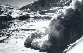
Powder-snow avalanches are one of several forms of snow or ice avalanches. It is known that peculiar conditions must be fulfilled and combine together in order that such avalanches can form; so they are generally a rare phenomenon. But once they occur, these avalanches often reach respectable sizes, amongst the biggest avalanching events that occur in the geophysical environment (see Fig. 1). When they arise in inhabitated regions, they often constitute catastrophic events, producing considerable damage both to property and the lives of people.
An ice avalanche which developed into a powder-snow avalanche on Mount Tilicho, Nepal. This photograph demonstrates the whole avalanche path with the steep part on the right, a kink zone in the middle and a flat run-out zone on the left. (Photograph by G. Kappenberger.)
In the Swiss Alpine regions, the last period of heavy concentrated snowfall occurred in the winter of 1983-84; several powder-snow avalanches were reported with in 1 d (SFISAR, 1984b). Thus their occurrence is seldom and episodic, and observation is difficult let alone the impossibility of field measurements. Nevertheless, the understanding of their physics is important, one reason being that mountainous regions are still further and further exploited; as a consequence, the potential danger due to possible avalanche events grows in parallel with it.
Snow avalanches may be crudely classified into two types, namely flow avalanches and powder-snow avalanches. In Nature, all possible forms between these extreme types are possible, but as soon as a considerable flow part exists within an avalanche, this flowing part usually produces higher pressures than the overlying snow cloud and the whole avalanche has therefore the character of a flow avalanche. In the run-out zone, however, the snow cloud may travel further or in a direction different from the dense flow (personal communication from H. U. Gubler), thus producing different kinds of damage in the different parts of its track. Physically, flow avalanches are akin to "laminar" granular flows but powder-snow avalanches manifest themselves as turbulent two-phase boundary-layer flows with the particles suspended in air. Flow avalanches can be further classified as slab avalanches and loose snow avalanches, depending on the cohesion of the original snowpack. By contrast, a powder-snow avalanche never develops directly from a snowpack at rest, but is always formed from a flow avalanche by processes that are in their details still not understood. Shear instabilities and/ or impact processes may play a role. The transition from flow avalanches to powder-snow avalanches occurs quite seldom and knowledge about this process and, incidentally also that of powder-snow avalanches, is much scarcer than that of flow avalanches.
The first mathematical description of avalanching motions is due to Reference VoellmyVoellmy (1955); he regarded an avalanche as a one-component fluid and established a hydraulic theory with two resistive force contributions, one of Coulomb-type in which the shear force is proportional to the normal force and the other of viscous type in which the drag was assumed proportional to the velocity squared. This allowed him to treat both flow avalanches and powder-snow avalanches using the same model by a change of the value for the drag coefficient. Since Voellmy’s pioneering work, his model has undergone several improvements. (Reference SalmSalm 1966, Reference Salm1968) and (Reference Perla, Cheng and McClungPerla and others 1980, Reference Perla, Lied and Kristensen1984) sharpened the numerical values of the frictional parameters, and Reference Shen and RoperShen and Roper (1970) extended Voellmy’s model to two dimensions. Many new ideas were introduced by Reference Tochon-Danguy and HopfingerTochon-Danguy and Hopfinger (1975) and Reference Hopfinger and Tochon-DanguyHopfinger and Tochon-Danguy (1977). They formulated local balances for mass and linear momentum, and integrated these laws over the height of the avalanche. In this way they obtained a set of equations governing the steady motion of the streamwise mean velocity and the avalanche height of flows from a steady source. This model was altered or extended by Reference Beghin, Hopfinger and BritterBeghin and others (1981) and Reference Beghin and BrugnotBeghin and Brugnot (1983) to apply to short, finite-mass avalanches undergoing transient processes. All these cited models are based on a density current rather than a two-phase concept and do not naturally incorporate a phase-separation concept. Consequently, their use is restricted to the steep part of an avalanche track, where phase-separation effects are of marginal importance. Investigations in the run-out zone of a powder-snow avalanche, however, have to deal with just these phenomena, which explains why a two-phase concept is urgent. Such a model was presented by Reference Scheiwiller and HutterScheiwiller and Hutter (1982), Reference ScheiwillerSchei-willer (1986) and Reference Scheiwiller, Hutter and HermannScheiwiller and others (1987). In a two-phase description, both mass and momentum balances are formulated for each of the phases and their interaction is accounted for by the mutual interaction force. It must be prescribed by a constitutive relation, and its functional form will critically determine the suitability of the mathematical description with regard to the sedimentation process. Because little is known about these processes, adjustment by experiments is significant.
Along the boundaries, air entrainment is modelled, but snow entrainment from the ground is not reproduced in our experiments. Both processes could be modelled computationally. Since this boundary-layer suspension flow is highly turbulent, the equations have to be time-averaged and the set must be closed by a turbulence-closure model. Reference ScheiwillerScheiwiller (1986) has chosen the k-E model. The mathematical formulation has also been published in Reference Scheiwiller, Hutter and HermannScheiwiller and others (1987).
Each model of a natural process must be corroborated by field data, preferably by obtaining data from the process itself or, if not possible, by laboratory experiments. For powder-snow avalanches, so far there has been no possibility of acquiring data from field experiments and even more so the generation of these avalanches in a systematic manner is far from being possible.Footnote * Accord-ingly, if progress in understanding the physics and describing mathematically the two-phase flows is to be made, powder-snow avalanches must be simulated in the laboratory. Once such an experimental set-up is established, a simulation has many advantages: there is no limitation in the number of experiments that are performed; initial and boundary conditions can be systematically modulated with no apparent danger to anyone involved in the experiments. It is clear that finding an appropriate simulation is a difficult task. Also, it should be no surprise that, according to the different theoretical approaches cited above, different simulation techniques were presented. Reference Tochon-Danguy and HopfingerTochon-Danguy and Hopfinger (1975) employed a density, gravity or turbidity-current concept and performed experiments in which the avalanche consisted of a heavy fluid that was dispersing in a lighter one. His set-up was later used by Reference Beghin and BrugnotBeghin and Brugnot (1983). In our case, because we regarded phase separation as important, a two-phase simulation was needed. The respective experimental arrangement was established by Reference ScheiwillerScheiwiller (1986), Reference Scheiwiller, Hutter and HermannScheiwiller and others (1987), and later amended and extended by Reference HermannHermann (1990). So far, more than 1000 experiments have been performed with this set-up. This paper presents some of the findings and conclusions that were reached from these runs.
Experimental Installations and Measuring Procedure
In our set-up, powder-snow avalanches are simulated by the turbulent suspension flow of polystyrene particles in water. All details relating to the simulation itself have been described by Reference ScheiwillerScheiwiller (1986) and Schweiwiller and others (1987). Since changes have been made in the measuring procedure but not in the simulation process, the reader is referred to these publications, and only a brief overview will be added here. Important for the interpretation of the experimental data at the laboratory scale and their transfer to the dimensions of a real avalanche in Nature are the laws of similtude, also described in Schweiwiller (1986).
Similarity is preserved by the conservation of (1) densimetric Froude number and (2) the ratio of downstream velocity to free-fall velocity. Table 1 provides a list of the orders of magnitude of the physically important quantities and the deduced dimensionless numbers as they appear in Nature and in the laboratory. Figures 2 and 3 show the experimental set-up, consisting of a water tank with dimensions of 5m × 4m × 2 m and a Perspex front, a submerged chute with kink and run-out zone, a cylindrical tank in which the suspension was prepared and from which avalanches were generated, and the equipment for recording measurements. The avalanche track is confined by Perspex side walls, which follow the chute to the kink zone and down to the run-out zone. Using them, a channelized flow is obtained. It is possible to remove the side walls in the run-out zone for the simulation of avalanches which flow from a narrow steep valley out into a plain (see Fig. 4). Contrary to what occurs in Nature, the avalanches in the laboratory simulation start as powder-snow avalanches; this is so because a water-particle suspension is released into the channel through a tube and diffuser from the suspension generator. This apparatus prepares a well-defined mixture of polystyrene powder and water, and controls every ingoing and outgoing quantity, i.e. initial concentration, initial speed (at the nozzle) and the behavior of these over the course of time. During an avalanche run, while the water-particle mixture is fed to the orifice, fresh water is fed into the suspension generator to maintain the nozzle pressure; this results in an approximately constant flow velocity at the inlet and a diluting concentration. In spite of this, observations have shown that the concentration can also be held constant for a time at least sufficiently long for the duration of the experiment; hence quasi-stationary suspension flow prevails for about 40s.
A general view of the water tank with the submerged chute, kink zone and run-out zone. The ladder gives an estimate of its size. (Photograph by F. Hermann.)

Schematic view of the experimental set-up. Within the water tank are the chute (Ch), the kink zone (K), the plane run-out zone (P) and the transducer array (T). Outside are a mixing apparatus (M),a computer (C) and the recording electronics (RE). The chute inclination angle is a, the kink angle is β, the measuring positions are indicated by italic numbers and letters, 1, 2, A and B. Position 1 is 1 m and position 2 is 1.5 m away from the inlet. The other positions are defined with respect to the end of the run-out zone; position B is there, while position A is 1 m to the left. The distance between positions 2 and A depends slightly on the kink angle and is β approximately 50 cm.

The side walls of the run-out zone may be removed, thus allowing sideways spreading of the avalanche. (Photograph by F. Hermann.)

Typical dimensions and dimensionless numbers in Nature and in the laboratory

In the resulting flow, particle velocity and concentrationFootnote * distributionsare measured by an ultrasonic technique. A small burst of a few wavelengths is transmitted into the fluid; it is reflected and scattered by the moving particles, and the reflected signal at the receiver suffers variations both in frequency and amplitude. The analysis of these echoes results in a mean velocity and mean concentration of all the particles within the sampling volume. Because the ultrasonic beam has negligible spreading, the size of this volume is given by the length of the burst and the diameter of the transducer. It has the shape of a disk, 7 mm in diameter and 0.5 mm in height. Because the incoming echoes originate from a number of distances in the direction of the beam, the total echo of the burst must be a continuous signal from all these distances. With a Sample-and-Hold circuit, a specific distance can be selected; it is chosen as a compromise between a small influence of wave scattering (which leads to a short distance) and a small influence of the measuring devices on the measured current (which would favor large distances). We have fixed it to three times the diameter of the transducer.
The sharp-bundles beam allows several transducers to work together in the same experiment without sensible interactions between themselves. An array of four transducers was used for the experiments, coupled with a specially designed electronic unit, containing the required electronic circuits and a small computer for signal analysis.
The numerical simulation of the avalanches will be two-dimensional; such a plane-flow simulation is approximately achieved by the chute experiments, if the measurements are taken in the middle of the chute. Two procedures were followed: in the first, profiles are taken along a line perpendicular to the chute floor; in the second, so-called "time sections" are recorded of which details will be described below. A profile is generated with the aid of a stepping motor that pulls the transducer array through 16 positions at different heights within the avalanche. The time required for gathering a profile depends on (1) the pulling speed, (2) the time for data sampling, and (3) the number of transducers. A long measuring time of several seconds limits measurements to the quasi-stationary parts of the avalanche, i.e. the avalanche body. To obtain data from the very turbulent avalanche head (see Fig. 5), either the measuring time must be reduced or a new procedure be applied. Previous measurements with only one transducer suffered severely from the restriction and led to the construction of the four-transducer array and its electronic support. This allowed measurements in the whole avalanche, both body and head, by employing the previously cited method of time sections.
A typical powder-snow avalanche consisting of a completely turbulent avalanche head and a quasi-stationary avalanche body. A typical velocity profile is shown.

A time section (see Fig. 6) consists of a series of profiles taken at the same place in equidistant time intervals with spatially fixed transducers. As the avalanche moves by, a time section collects data from different regions within the avalanche and, the velocity distribution known, could be back-calculated into a longitudinal section. For reasons of economy, the transverse resolution of a partial profile within a time section is half as high as that of a single profile and consists of measurements at eight different depths. Sixteen such profiles are compiled into a time section. Single profiles are taken in the middle of the avalanche head and in the avalanche body; time sections are started immediately before the avalanche front reaches the four sampling volumina, so that the processes preceding the front are also covered by the measurements. Since the time interval between consecutive partial profiles in a time section can be chosen arbitrarily, different kinds of time sections can be generated. A long time interval leads to "general views" of the avalanche, while a short interval results in "close-ups" of the regions near the avalanche front. As will be seen later, these close-ups reveal insight into new and interesting features.
Time sections are generated with a fixed transducer array when the avalanche moves by, as indicated by the arrow. The position of the actual measuring volume is denoted by (X), while previous positions relative to the moving avalanche are represented by

The presentation of the data is given in two forms: single profiles are shown as φ–h plots, where φ stands for the investigated quantity and h for the depth; for time sections, the values for the investigated quantity are filled into a ht field, interconnected by a spline function and coded into color (see later, Figs 14–17 and 19).
The highly turbulent nature of the avalanche requires ensemble averaging over seven identical experiments. Figure 7 shows single experiments and averages for a velocity and density profile. The development of an avalanche is recorded at four measuring positions along the avalanche track as indicated in Figure 3. Position 1 lies l m below the inlet and position 2 is located 50 cm downstream. Immediately after it, the kink zone follows; its end is both the beginning of the run-out zone and the location of position A. The last position, B, is located at the end of the run-out zone, 1 m downstream of position A.
Single profile measurements (top) and their ensemble average (bottom) of velocity (left) and density (right). Ensemble averaging of seven single experiments turned out to be sufficient to eliminate individual turbulence eddy effects. The parameters of these measurements are α = 40°,β = 55° in position B.

Before experiments were run in a systematic manner, some preliminary experiments were performed to determine the most interesting places within the avalanche track (Reference Hermann and ScheiwillerHermann and Scheiwiller, 1987). Soon it became clear that the kink zone plays a crucial role. In that region an avalanche loses a considerable proportion of its particles by sedimentation, which suggests important consequences to the further flow beyond it. Figure 8 shows this sediment layer after three avalanches had passed.
A large deposit of particles is generated after the successive release of three avalanches.

The systematic experiments covered a wide range of chute inclinations and kink angles as shown in Table 2. For every combination of these two angles the type of measurements undertaken is indicated.
Table 2. Combinations of a and B where measurements of different types were performed, hp denotes head profile, bp stands for body profile and ts mean time section

Results
This work was mainly directed towards three different goals: the first was to determine a run-out zone for powder-snow avalanches and to find the essential physical dependencies within it; the second one consisted of detecting the dominant physical processes in the kink and run-out zones, and the third was the establishment of a set of laboratory measurements for testing numerical models which implement an avalanche theory. The results show that the first goal has only been partly achieved, because the results at position B show that the run-out distance is definitely larger than provided for by the experimental set-up. So, run-out distances cannot be measured with our set-up and our initial conditions; they must be estimated from the present data. As for the second goal, these data provide much information, a substantial part of which will be explored in this paper. In this presentation, we follow the avalanche along its track: the kink zone is treated first, followed by results from the runout zone. Comparison of the data with computational results is deferred to a further paper.
The Kink Zone
The kink zone is the location of intense sedimentation. The deposit after seven successive avalanches has been measured during systematic measurement runs; it shows that up to 70% of the initial mass deposits into the kink zone, if the chute is steep enough to prevent deposition in the chute. Clearly, such sedimentation must manifest itself in the concentration measurements at positions 2 and A. These measurements are restricted to the avalanche body and Figure 9 shows the velocity and density profiles taken at a chute angle at the steep part of 35°. Results for the whole avalanche track are also shown in this plot, starting at position 1 on the left and ending with position B on the right. After position 2, the plots are split into three groups according to the three different kink angles for which experiments were performed. The upper half of the figure collects the velocity data; overall density is shown in the lower part. As expected, a substantial reduction of density can be observed between positions 2 and A, this reduction being as large as a quarter or even more. The shapes of the profiles change from more or less triangular in positions 1 and 2 to alomost uniformity in positions A and B. It is evident that the major part of the deposit stems from regions near the bottom (a considerable part of it may even come from regions just above the bottom which are not accessible to the measurements).
Profile measurements in the avalanche body for a = 35°. Velocity data are plotted in the upper half, and density data in the lower half of the figure. The profiles cover the whole avalanche track from position 1 (left) to position B (right). After position 2, the figure splits into three possible paths depending on the kink angle B, which is 35 (top row), 45 (middle row) or 55° (bottom row). As explained in the text, the most striking features are a reduction of the maximum in the kink zone, which is to a certain extent compensated by a redistribution of the velocity profile and a significant density reduction.

The velocities are also affected by the kink. A comparison of the profiles at positions 2 and A shows a qualitative difference in the occurrence of the maximum velocity. An analysis of all the velocity data gives a mean reduction of about 60%, depending (slightly) on the kink angle (67% at 35°, 56% at 55°;). The same comparison between the integrals over depth of the velocity profiles gives a much less pronounced reduction. It follows that velocities in the kink zone are rather redistributed than reduced. However, both the velocity and the density profiles do not provide clear indications as to the processes in the kink, which generate sedimentation. With the aid of thin-section photographs, a qualitative evaluation is nevertheless possible (see Fig. 10). The particles are shown as white lines, indicating their movement.Footnote * Immediately above the deposit, a zone of reduced velocity can be seen. We suggest that a layer of small clockwise vortices is at work here and produces a considerable reduction of the boundary-layer velocity.Footnote * This facilitates sedimentation in this zone. A second, large vortex can be seen at the upper edge of Figure 10. This vortex appears on almost every photograph taken in this region and it seems to be stationary. Its function is to drive the already dense layers at small and medium height towards the ground, i.e. the already existing deposit. A schematic view of these vortices is given in Figure 11.
Particle tracks in the kink zone show the existence of small vortices near the ground and a large one at the upper boundary of the avalanche. (Photograph by F. Hermann.)

Schematic view of the positions of the vortices within the kink zone.

In steep chutes (a > 35°), an additional effect is active; in these cases there is a dense current close to the bottom, since a is larger than the angle of response of the non-cohesive material. All the particles which settle at lower inclination angles (see Fig. 13) form now this current, partly flowing and partly in suspension, which cannot be measured because of its small height. (The minimal height at which a transducer can operate is about 1 cm above the ground. This is mainly a problem of its position but also of its diameter.) All the material transported in this thin layer is deposited in the kink zone. Its volume can be estimated when results from different chute angles are compared. At low angles, where sedimentation in the chute itself is possible, the deposit in the kink zone is reduced by the amount brought in by this density current. Figure 12 shows a sequence of photographs made during an experiment with a high-speed camera, where the formation of sedimentation can be observed, and Figure 13 gives an example of the measured deposits after seven avalanches versus the chute angle with a fixed kink-zone angle of 45°. Compared to real avalanches, the existence of such dense flow at ground level is realistic, since many avalanches are of a mixed type rather than pure powder-snow avalanches, as mentioned above. In the mathematical model, however, such a flow has not yet been incorporated, but it could be done with some effort by changing the lower boundary condition.
The passing of an avalanche in the kink zone captured by a high-speed camera (l0 frames/s). In frame (c) a dense layer near the bottom appears, which forms the deposit. Wave patterns on its upper boundary can be seen in frame (d). (Photographs by F. Hermann.)

The measured deposits of seven avalanches versus the chute angle a at a kink angle B= 45°, split into three parts of the avalanche path (broken lines). The full line is the sum of the deposit. The total material released was approximately 18000 cm3. For a < 35°, deposition in the steep part of the chute is possible, whereas at higher inclinations this amount of material is concentrated in the kink zone.

The Run-Out Zone
In the run-out zone, since this is the zone of primary interest, a large body of data is available, both from the avalanche body and from the avalanche head. The analysis of the measurements discloses several effects which will be discussed below. They are:
The general structure of velocity and density distributions in the avalanche.
A reduction in velocity near the ground.
An overall reduction of the density.
The existence of a precursory zone ahead of the avalanche density front where fluid movements are high.
The deceleration of dense regions within the avalanche head.
The specific kinetic energy or stagnation pressure and the calculation of avalanche danger.
The discussion is based on the illustrations shown in Figure 9 and 14–19 that were obtained by a detailed data analysis.
General Structure of Velocity and Density Distributions
Figures 14 and 15 show the velocity (top) and density (bottom) distributions in colour codes of an avalanche in position A (Fig. 14) and position B (Fig. 15) versus time as the avalanche passes the position. These plots have been generated from time sections as described earlier. The time interval between consecutive measurements is 1.5 s in position A and 1.0 s in position B, the time-scale being indicated on the abscissa. The ordinate gives the height above ground, ranging from 0 to 24 cm. A coloured bar at the right interprets the coding for the desired quantity, ranging from 0 to 20cms−1 for velocities and from 0 to 12 gl−1 for densities (i.e. from 0 to 10−2 in terms of volume concentration). A comparison of velocity and density plots shows a remarkable difference in what might be the duration and, consequently, the spatial dimension of the different zones. In the velocity plot, the structures (i.e. areas of equal colour) are larger and their gradients are in general small. As an example, at a height of 6 cm, a velocity of c. 8 cms−1 persists for 20s. Avalanche head and body are distinguished by the vertical extent of higher velocities and densities in regions above 12 cm. The avalanche body shows a quasi-stationary behaviour as assumed. Contrary to the velocity plot, the density plot shows several distinct maxima, one near the ground, two at medium heights and one near the upper margin of the avalanche head. Two other, smaller maxima are visible in the avalanche body. These maxima appear to be small in their spatial dimensions and manifest themselves as strong and sharp peaks. Comparison of profile measurements and time sections also provides information about the reliability of the profiles. Since measurements through profiles are not automatically initiated but released by eye and hand,Footnote * there is a random component in their position relative to the avalanche head or body. The time sections now show that the velocity field changes much slower than docs the density field. We may therefore assign a higher reliability to the velocity profile than to the density profile, since the exact release time is not known.Footnote * This difference in reliability is more pronounced in the avalanche head than in the avalanche body because density maxima are rare in the latter.

The Reduction of the Velocity Near the Ground
A comparison of velocity data between positions A and B, whether for profiles such as those in Figure 9 or time sections as in Figures 14 and 15, shows that the most conspicuous variations take place in the first centimetres above the ground. Here, a pronounced reduction by a factor of up to 4 may be seen in contrast to the remainder of the avalanche, where velocities change much less (compare the yellow-red regions near the abscissa in Figure 14 with the blue in Figure 15). There are two possible explanations for this decrease: the first is the influence of ground friction (which is negligible in the steep part of the track), and the other one is a late influence of the kink due to inertia. Which one of these is acting (if at all) is still an open problem, which has to be solved by further experiments. The question could be answered with avalanches containing less initial energy (or the same avalanches in longer run-out zones). In such a case, inertia would produce a zone of very low velocities near the ground followed by a zone of higher velocities at the end of the run-out zone. On the other hand, if ground friction were the dominant process, the velocity near the ground would decrease continuously.
The Redaction of the Density
Contrary to the velocity (which only suffers a substantial reduction near the ground), the density is substantially reduced between positions A and B. A comparison of the profiles in Figure 9 shows a reduction in the lower half of the avalanche depth which brings the profiles down to near uniformity. More information may be gained from the time sections (Figs 14 and 15). They show that a reduction taken place mostly between the maxima and less at the maxima themselves. These are not (or very faintly) affected in their values and only their extension in time is reduced. Long time sections show that the small maxima in the avalanche body disappear, and the body shows a small, nearly constant density which agrees well with the profile measurements. For the attenuation of density, some calculations have been carried out with the profile measurements for B = 35. On the other hand, comparison of the integrated density profiles at different chute inclinations a in positions A and B allows the definition of a mean density loss in the run-out zone. Table 3 gives the values for the various inclinations and their arithmetic mean value for both body and head profiles.Footnote * As an interesting feature, the mean density attenuation is the same for body and head, and it does not show a dependence upon a.
Density attenuation factors between positions A and B for various inclination angles a. and a kink angle B = 35. The lefthand column shows the values obtained from body profiles, the righthand one those of the avalanche head. Their average is approximately the same

The Fluid Movement Preceding the Avalanche Front
Figure 16 and 17 correspond to Figure 14 and 15, but they have been obtained by using a different recording interval. They disclose a better resolution in time and may provide details which are averaged out or hidden in the time sections of Figure 14 and Figure 15. Such detail is the shape of the density maxima. In Figure 16, the maximum consists of several peaks while the corresponding region in Figure 14 consists of only one maximum. The most striking feature of these new plots is the difference in the velocity and density front.It is clear that the visible edge of the avalanche (see Fig. 18coincides with the density front. So, all the velocity data that are recorded before this front arrived at the measuring position must stem from water movements, made "visible" by small impurities in the water. By comparing the data betwen positions A and B, the reader may find that this zone of fluid movement without particles grows within the run-out zone. The strange form of this precursor in position A may be astonishing; it is due to the influence of the nearby kink and disappears in the run-out zone. Preliminary sampled time sections of velocity and density in the steep part of the chute also show a small precursor which has a shape similar to that at position B, The velocities in the precursor show about the same values as those within the avalanche. This provides some guidelines as to the formation of such a precursor. It might be due to fluid that is accelerated by the particle in the avalanche track and less decelerated in the run-out zone. This precursor was also found by Reference Tochon-Danguy and HopfingerTochon-Danguy and Hopfinger (1975) in their experiments. For natural events, it has been reported by Reference Nishimura, Narita, Maeno and KawadaNishimura and others (1989) and Norem (personal communication); it is also well known to foresters and mountaineers.

The sharp front of an avalanche. It corresponds to the density front in 16 or 17.

The Deceleration of Dense Regions in the Avalanche Head
Let us study next the density and velocity distributions within the avalanche head as they appear in Figures 16 and 17. In position A, density and velocity are correlated insofar as the maximum velocities occur at the same time and at the same height as the density maxima (within a proper avalanche, the precursor may be faster). This is no longer the case in position B; rather the contrary is observed: the zones of maximum density are now correlated with relative minima in the velocity field. The physical interpretation of this phenomenon is inter-phase friction. Since the avalanche in the run-out zone is moving uphill (the negative inclination angle is 20° in this example), gravity has a component opposite to the mean flow direction. The corresponding buoyancy force acts on the particles and the fluid is decelerated by inter-phase friction. The fact that only the dense parts in the avalanche head show a discernible deceleration while the velocity of the regions with lesser concentration essentially maintain their velocity makes it likely that a non-linear relation between concentration and inter-phase momentum transport is active. Scheiwiller’s proposal (1986)
with m as momentum transfer, c as concentration and u as velocity is linear in concentration, but a power law seems to be more realistic:
The present data base is insufficient for an evaluation of the exponent. Further time sections are needed with a finer grid and more points at least along the time axis, a requirement which is presently beyond the hardware capability of our electronic equipment but it might be achieved in the near future.
Energy Considerations, Maps of Endangered Zones and Estimation of the Length of a Run-Out Zone
Two parameters are taken into account for the determination of areas endangered by powder-snow avalanches: dynamic (stagnation) pressure of the avalanche (the definition being pv 2/2) and a mean repetition time of the avalanche event. In Switzerland, there are such guiding rules (SFISAR, 1984a) for the dynamic pressure, the limit being set at 1.5 kPa for absolute endangered zones and 0.5kPa for unprotected zones.Footnote * Pressures between these values are found in zones which are declared as potentially endangered, but they may be explored and managed using appropriate precautions. With the assumption of equal velocity for both phases, the distribution of dynamic pressure can be calculated from the velocity and density fields via the formula
where p f and p p are the material densities of the fluid and the particles respectively, v is the velocity and c is the particle concentration. As a second step, the experimental data may be expanded to natural sizes through the laws of similtude (for the ratios of velocity and length scales used in these calculations (see Table 1); the density was back-calculated into volume concentration, thus giving a new density by inserting the material density of ice and air instead of those of polystyrene and water, respectively). As a result of this procedure, Figure 19 shows calculated time sections for dynamic pressure transferred to natural size. This plot is a direct re-interpretation of the previous Figures 14 and 15 and provides information about the pressures which must be expected with a powder-snow avalanche. In position A, two pressure maxima may be discerned, one in the middle of the avalanche head and the other one near the ground. It is clear that, overall, the second one affects forests and buildings; however, also those parts between the pressure maxima lie well above the limit of 1.5 kPa, so the whole zone has to be considered as dangerous. In position B, the distribution has changed insofar as the pressure maximum near the ground has disappeared. Up to heights of about 30 m above the ground, the pressure is now below the limit of absolute danger. This conflicts with the classification of such an avalanche, because above this height the pressures are still far higher than the limit set by the code. Based on this result, we suggest expanding the guiding rules for powder-snow avalanches by introducing an additional height parameter, e.g. to define an avalanche as dangerous if the dynamic pressure exceeds 1.5 kPa within 60 m above the ground.

It has already been mentioned above that in our setup the definition of a run-out distance of laboratory powder-snow avalanches is not possible by measurements. At present, the only way of obtaining an idea about it is to extrapolate the developments of both density and velocity distributions from the known data in positions A and B and to calculate from these extrapolations the dynamic pressure. This is done in Table 4 using the same values as in Table 3 and for a fixed kink angle B = 35, using body and head profiles in positions A and B, respectively. The first and second columns contain the values for the mean dynamic pressure, which are obtained by taking values from the velocity and density profiles as described above and averaging over the flow height. Column 3 shows their ratio. For the fourth column, we assumed that (i) this ratio remains the same and (ii) that an average dynamic pressure of 1 kPa may be considered as low enough to ensure no danger within a certain height (e.g. 60 m; see above). Under these conditions, a distance factor (the runout distance equals this factor times the distance between positions A and B) may be calculated; it is shown in the last column. The table indicates a drastic increase in the estimated run-out distance with the chute inclination, but it should be taken into account that the constant kink angle produces a changing inclination of the run-out zone, ranging from -10 to 15 and thus amplifying the effect. It may also be seen that the run-out distances for the avalanche head (in the lower half of Table 4) are sensibly longer than those for the avalanche body (upper half). This is in accordance with the observations using time sections. These show that the tendency of the density distribution is towards isolated density maxima which remain intact a long time. Since velocities decrease slowly, these isolated density maxima still correspond to locations of high pressure, but these regions are also well away from the ground. It is therefore an open question how far these maxima must be considered in an avalanche code, but it is clear that the run-out distance for these maxima is longer than that for mean values. Another point of importance is a possible lateral spreading of the avalanche which occurs when a channelled avalanche surges into an open valley. In such a configuration (see Figure 4 for a preliminary experiment), even the short run-out zone in the set-up shows effects as described above and the run-out distance would be considerably reduced.
Estimated run-out distances (in units of the distance between positions A and B) from the averaged dynamic pressures in positions A (first column) and B (second column) for various inclination angles a. at a fixed kink angle B = 35°. The upper half of the table shows the values obtained from the body profiles, and the lower half those from the head profiles

Conclusions
The above-described experiments demonstrate the usefulness of a laboratory simulation of powder-snow avalanches. So far, a reliable data set has been obtained and interesting features for the behaviour of powder-snow avalanches have been found. One of the important unsolved problems is the measurement of the fluid velocity distribution, which plays a crucial role in the modelling of momentum transfer. Another avenue would be to follow the extension into three dimensions. A possible configuration is shown in Figure 4, where a channelled avalanche flows into an open plain — a situation which occurs quite often in Nature. Preliminary experiments for such a configuration have shown that the density in such an avalanche decreases faster when compared with the channelled one with velocities remaining in the same order of magnitude. Qualitatively, the observed density decrease follows the path outlined above: the avalanche head consists of several density maxima which are no longer connected between themselves.
Acknowledgements
This work was made possible by Professor Dr D. Vischer, Director of the Versuchsanstalt fur Wasserbau, Hydro-logie und Glaziologie (VAW), who provided all facilities and equipment. His continuing support and generosity is gratefully acknowledged. We thank Professor C. Jaccard, Dr B. Salm and Dr H. U. Gubler from the SFISAR for much help and fruitful discussions. C. Bucher helped in planning and constructing the experimental set-up; J. Hermann, K. Dick and B. Junger assisted in performing the experiments.
We thank S. Basler and U. Moser for construction of the transducers and the copyright of the plans of the ultrasonic devices, and J. Forrer for his support in the construction of the electronic curcuits.
During this work, F. Hermann was financially supported by the Swiss National Science Foundation and the Swiss Federal Institute for Snow and Avalanche Research.
The accuracy of references in the text and in this list is the responsibility of the authors, to whom queries should be addressed.


