


1. Introduction
Low-Reynolds-number motion of objects near surfaces is found across a wide range of engineering, microfluidic and biomedical applications. In particular, when surfaces are in close proximity, considerable research has focused on the study of the fluid and structure interactions that occur within the lubrication layer (Hamrock, Schmid & Jacobson Reference Hamrock, Schmid and Jacobson2004). The dynamics can be quite varied, and include hydrodynamic forces and velocities for spherical particles moving near planar walls (Goldman, Cox & Brenner Reference Goldman, Cox and Brenner1967a,Reference Goldman, Cox and Brennerb), spheroidal particles in shear flows near a solid wall, as studied using a variant of the boundary integral equation method (Gavze & Shapiro Reference Gavze and Shapiro1997), and particle sedimentation near a plane wall accounting for weak non-Newtonian and inertial effects (Becker, McKinley & Stone Reference Becker, McKinley and Stone1996). Dynamics frequently involve cylindrical geometries, such as in the determination of the drag forces on a microcantilever oscillating near a wall (Clarke et al. Reference Clarke, Cox, Williams and Jensen2005), the design and optimization of viscous micropumps (Sen, Wajerski & Gad-el Hak Reference Sen, Wajerski and Gad-el Hak1996; Day & Stone Reference Day and Stone2000; Choi et al. Reference Choi, Lee, Choi and Maeng2010), motion of air bearings, including effects of fluid compressibility (Witelski Reference Witelski1998), and the circular swimming motion of Escherichia coli bacteria near a solid boundary (Lauga et al. Reference Lauga, DiLuzio, Whitesides and Stone2006) and the motor torque of such bacteria (Das & Lauga Reference Das and Lauga2018), among many others. In almost all, if not all, such cases, the cylinder is modelled as infinite. The present paper focuses on the dynamics of three-dimensional (3-D) finite cylindrical rods translating and rotating near a rigid planar wall.
The classic solution for the rotation of a cylinder in a viscously dominated flow was calculated by Jeffery (Reference Jeffery1922) using bipolar coordinates to solve the two-dimensional (2-D) Stokes flow problem. Jeffrey & Onishi (Reference Jeffrey and Onishi1981) extended this work to consider the 2-D flows associated with rotation and translation of an infinite cylinder both parallel and perpendicular to a nearby plane wall, which they solved analytically using a stream function formulation of the Stokes equations, along with the bipolar coordinate representation. Variations on this problem have been studied, including theoretical prediction of the drag force on a zero-thickness disk translating towards a plane wall (Davis Reference Davis1993) and the consequences of slip conditions due to superhydrophobic surfaces (Kaynan & Yariv Reference Kaynan and Yariv2017; Schnitzer & Yariv Reference Schnitzer and Yariv2019). Also, Crowdy (Reference Crowdy2011) rederived the results of Jeffrey & Onishi (Reference Jeffrey and Onishi1981) without approximation and developed an explicit nonlinear dynamical system for treadmilling swimmers. The effect of non-zero Reynolds number for the motion of a cylinder rolling along a wall, both with and without a gap, has also been reported (Merlen & Frankiewicz Reference Merlen and Frankiewicz2011). More recently, studies have expanded on the theories of Jeffrey & Onishi (Reference Jeffrey and Onishi1981) to include additional coupled physics, such as the effects of soft interfaces on the fluid dynamics in the lubrication layer and the forces that originate due to non-conforming contacts (Skotheim & Mahadevan Reference Skotheim and Mahadevan2004, Reference Skotheim and Mahadevan2005; Salez & Mahadevan Reference Salez and Mahadevan2015; Rallabandi et al. Reference Rallabandi, Saintyves, Jules, Salez, Schönecker, Mahadevan and Stone2017; Saintyves et al. Reference Saintyves, Rallabandi, Jules, Ault, Salez, Schönecker, Stone and Mahadevan2020).
One, perhaps surprising, result from the original analysis of Jeffrey & Onishi (Reference Jeffrey and Onishi1981) is that the hydrodynamic force on an infinite cylinder moving near a wall is independent of its rotation rate and, by symmetry, the hydrodynamic torque on the cylinder is independent of its translational velocity. A consequence of this fact is that there is no coupling between rotation and translation for an infinite cylinder translating near a planar wall in the absence of an externally applied torque. However, finite objects such as a sphere moving near a planar wall will, in fact, respond by both rotating and translating when either experiencing an external force, to remain torque free, or an external torque to remain force free. For the case of a finite-length cylinder then, these facts suggest that external forces or torques, for the cases of lateral translation and rotation, respectively, lead to a coupling between translation and rotation and originate due to end effects. In a recent experimental study of a finite-length cylinder sliding down a soft incline while free to rotate, the 2-D solution for an infinite cylinder, derived by Rallabandi et al. (Reference Rallabandi, Saintyves, Jules, Salez, Schönecker, Mahadevan and Stone2017) using the Lorentz reciprocal theorem, showed quantitative discrepancies with the experimental results (Saintyves et al. Reference Saintyves, Rallabandi, Jules, Ault, Salez, Schönecker, Stone and Mahadevan2020). This discrepancy led to the development of a new theory that considers elastohydrodynamic torque as well as the viscous friction induced by the ends of the cylinders. Saintyves et al. (Reference Saintyves, Rallabandi, Jules, Ault, Salez, Schönecker, Stone and Mahadevan2020) experimentally and theoretically showed that the cylinder's end-effects play a non-negligible role in the case of motion of a finite-length cylinder and motivate this work.
Finally, several other important works have explored various aspects of particle motion near boundaries using slender-body theory and other asymptotic methods, some of which examined similar configurations to that of the present study. For example, Russel et al. (Reference Russel, Hinch, Leal and Tieffenbruck1977) used slender-body theory to model the glancing and reversing tumbling of inclined rods settling close to a plane wall. A more recent work by Barta & Liron (Reference Barta and Liron1988) built on this work using a singularity method in two regimes, where the body–wall distance was the same order as either the body length or the body width. Youngren & Acrivos (Reference Youngren and Acrivos1975) presented a general numerical approach to calculate the Stokes flow past general shaped bodies such as cylinders which can take into account the end effects. They applied this method to a cylinder translating parallel to its axis. Katz, Blake & Paveri-Fontana (Reference Katz, Blake and Paveri-Fontana1975) also considered the translational motion of rigid slender bodies near a boundary in the limit where the radius of the body is much less than the separation to the wall, which in turn is small compared with the radius of the body. The slender body motion has also been considered near a flat fluid–fluid interface in contrast to a solid plane wall (Yang & Leal Reference Yang and Leal1983). De Mestre & Russel (Reference De Mestre and Russel1975) used slender-body theory to calculate the total drag on rotating and translating rods near a plane wall for body–wall separations which are large relative to the rod radius. Two of the classic theoretical works on slender-body theory are by Batchelor (Reference Batchelor1970) and Cox (Reference Cox1970), who used the slender body theory to calculate the Stokes flow past slender bodies of arbitrary cross-section.
Another closely related work to the present study is that of De Mestre (Reference De Mestre1973), which calculated the drag on a cylinder travelling parallel to a plane wall using slender-body theory. The distinction from the present work is that those results are valid for cases where the distance to the wall is large relative to the cylinder length. One of the relatively fewer experimental studies is by Ui, Hussey & Roger (Reference Ui, Hussey and Roger1984), who measured the drag on cylinders travelling along their axis within a cylindrical container to quantify the wall effects. Mitchell & Spagnolie (Reference Mitchell and Spagnolie2015) used the method of images to model the sedimentation of prolate and oblate spheroids near an inclined wall and suggested the possibility of incorporating lubrication effects along the lines of those introduced in this paper. Lisicki, Cichocki & Wajnryb (Reference Lisicki, Cichocki and Wajnryb2016) derived an explicit relation for the correction to the bulk diffusion tensor of an axially symmetric colloidal particle due to a nearby plane wall. Finally, Koens & Montenegro-Johnson (Reference Koens and Montenegro-Johnson2021) determined the drag per unit length on a slender rod translating parallel to a wall which is valid for all separation distances. This was achieved through asymptotic matching to the results of both De Mestre & Russel (Reference De Mestre and Russel1975) and Jeffrey & Onishi (Reference Jeffrey and Onishi1981).
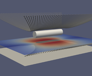
Here, we build on the work of Saintyves et al. (Reference Saintyves, Rallabandi, Jules, Ault, Salez, Schönecker, Stone and Mahadevan2020) and generalize their theory to consider rotation and translation, both parallel and perpendicular to a nearby solid planar boundary, of a finite-length cylinder (see figure 1). We use 3-D numerical simulations of the Navier–Stokes equations to calculate the viscous and pressure forces and torques exerted by the fluid on a cylinder for a range of cylinder lengths and cylinder-plane gap heights. We identify conditions where the end effects dominate and drive a qualitative deviation from the case of a 2-D infinite cylinder. In particular, in § 2, we develop theory based on the lubrication approximation within the gap region to calculate the resistance matrices for the cylinder motion in order to describe the relationships between the translational and angular velocities and the forces and torques, and we develop analytical expressions for the resistance components. Next, in § 3, we present the numerical methods used for the 3-D simulations, and we introduce representative results and flow behaviours. Then, we present a comparison between the theory and the numerical simulations in § 4, and show that the numerical results collapse to the theoretical predictions in the long- and short-cylinder limits. Finally, in § 5, we provide discussion and conclusions. Further validation of the numerical methods including the results of convergence tests can be found in the Appendix (A).

Figure 1. The geometrical configuration and coordinate system for a finite-length cylinder moving near a plane wall. We consider the parallel translation ( $U\neq 0$), rotation ( $\varOmega \neq 0$) and perpendicular translation ( $V\neq 0$) of a finite-length cylinder near a solid plane wall. The cylinder radius and length are $a$ and $L$, respectively, and the minimum gap height between the cylinder and the wall is $h_0$.
2. Theory
The classic solution for the low-Reynolds-number motion of an infinite circular cylinder near a plane wall is given by Jeffrey & Onishi (Reference Jeffrey and Onishi1981). This work introduced solutions for three cases: translation parallel to the plane; translation perpendicular to the plane; and rotation about the cylinder's axis. In each case the axis of the cylinder is oriented parallel to the plane. A key result of this work is that a force-free infinite cylinder rotating next to a plane wall does not translate, and a torque-free infinite cylinder translating next to a plane wall does not rotate. Here, we define the dimensionless gap height between the cylinder and the plane wall as  $\epsilon =h_0/a$, where $h_0$ is the minimum gap height and $a$ is the cylinder radius. The shear viscosity of the fluid is $\mu$, and the translational velocities parallel and perpendicular to the wall and rotational velocity of the cylinder are $U$,
$U$,  $V$ and $\varOmega$, respectively (see figure 1). Jeffrey & Onishi (Reference Jeffrey and Onishi1981) showed that the dimensionless torque per unit length (non-dimensionalized by $\mu \varOmega a^2$) resisting motion of an infinite-length cylinder rotating next to a plane wall is given by
 \begin{equation} \tau ={-}4{\rm \pi}\frac{(1+\epsilon)}{\sqrt{2\epsilon+\epsilon ^{2}}}. \end{equation}
Furthermore, they also showed that an infinite cylinder translating at speed  $U$ parallel to a plane wall experiences zero hydrodynamic torque and a total drag force per unit length (non-dimensionalized by $\mu U$) that is given by
 \begin{equation} f_\parallel{=}{-}4{\rm \pi}\log(1+\epsilon+\sqrt{2\epsilon+\epsilon^2})^{{-}1}. \end{equation}
In these cases, the cylinder either rotates due to the external torque per unit length but does not translate, or it translates due to the external force per unit length but does not rotate. Finally, Jeffrey & Onishi (Reference Jeffrey and Onishi1981) showed that the vertical force per unit length (non-dimensionalized by  $\mu V$) on an infinite cylinder translating at speed $V$ perpendicular to a plane wall is given by
 \begin{equation} f_\perp{=}{-}4{\rm \pi}\left[\log(1+\epsilon+\sqrt{2\epsilon + \epsilon^2}) - \frac{\sqrt{2\epsilon+\epsilon^2}}{1+\epsilon}\right]^{{-}1}. \end{equation}
Below, we will also need the relation of force and velocity experienced by a disk of radius  $a$ and zero thickness translating edgewise. Ray (Reference Ray1936) determined an analytical solution for the resistance force experienced by such a disk, and Davis (Reference Davis1993) generalized and expanded this result and presented the theoretical force as
 \begin{equation} F_\perp{=} \tfrac{32}{3} F_D, \end{equation}
where  $F_\perp$ is non-dimensionalized by $\mu V a$, and $F_D$ is a higher-order dimensionless force coefficient that has been derived by Davis (Reference Davis1993),
 \begin{align} F_D^{{-}1} = 1 - \frac{2}{{\rm \pi} (1+\epsilon)} + \frac{1}{3{\rm \pi} (1+\epsilon)^3} - \frac{3}{4{\rm \pi}^2 (1+\epsilon)^4} + \frac{7}{144{\rm \pi} (1+\epsilon)^5} + O\left(\frac{1}{(1+\epsilon)^6}\right). \end{align}
The above-mentioned works focus solely on the cases of infinite- or zero-length cylinders. Here, we focus our attention on the case of finite-length cylinders, as the importance of this geometric feature for cylinder motion near a wall was recently highlighted by Saintyves et al. (Reference Saintyves, Rallabandi, Jules, Ault, Salez, Schönecker, Stone and Mahadevan2020). Here, we generalize the work of Saintyves et al. (Reference Saintyves, Rallabandi, Jules, Ault, Salez, Schönecker, Stone and Mahadevan2020) and develop an analytical description for the motion of finite-length cylinders moving near solid planar walls ( $\epsilon \ll 1$) via a lubrication theory including the effects of the ends of the cylinder. In this way, translation and rotation are coupled.
2.1. Lubrication theory for a finite-length cylinder: wall-parallel translation and rotation
Here, we use lubrication theory to analyse the forces and torques on a finite-length cylinder rotating or translating close to a rigid wall, including end effects (see figure 1). The length of the cylinder is denoted by  $L$. The minimum separation distance between the cylinder and the wall is assumed small relative to the cylinder radius and the cylinder length, so $h_0/a = \epsilon \ll 1$ and $h_0/L \ll 1$, so that lubrication theory is applicable. The characteristic length scale along the gap, perpendicular to the axis of the cylinder $(x)$, is $\ell = \sqrt {2 a h_0}$, and the axial $(y)$ length scale is $L$. The ratio of these two quantities is $\mathcal {L} =L/\ell = L/(a \sqrt {2 \epsilon })$, which may be either large or small depending on the relative magnitudes of $L/a$ and $\epsilon$. Observe that $\mathcal {L}$ characterizes the aspect ratio of the lubricated region, and differs from the aspect ratio $L/a$ of the cylinder.
With these definitions, the gap between the cylinder and the fluid is approximated by the parabolic function  $h(x) \sim h_0(1 + x^2/\ell ^2)$, which is valid inside the lubricated region where $x = O(\ell )$. Then, the dimensional pressure $p(x,y)$ under a translating and rotating cylinder is governed by the Reynolds equation
 \begin{equation} \boldsymbol{\nabla} \boldsymbol{\cdot} (h^3 \boldsymbol{\nabla} p) + 6 \mu (U + a \varOmega) \frac{\partial^{}h}{\partial x^{}} = 12 \mu V, \end{equation}
where  $\boldsymbol {\nabla } = \boldsymbol {e}_x\partial _x + \boldsymbol {e}_y\partial _y$ is the gradient in the $xy$ plane. As is standard in lubrication theory, the pressure is nearly constant across the gap and is much greater than the pressure outside the gap, and so $p(x,y)$ must vanish outside the lubrication region. Along $x$, the outer edge of the gap is at $x = O(a) \gg \ell$, so $p$ decays smoothly as $x/\ell \to \pm \infty$. Along $y$ the gap width $h(x)$ diverges abruptly past the two end faces at $y= \pm L/2$ and so the pressure must vanish at these planes. Note that, in fact, there is a finite region outside of the edge of the gap where the pressure adjusts to the outer condition. We will later show that this region shrinks with the gap height, and so in the lubrication limit this leads to the boundary conditions
 \begin{equation} p(x \rightarrow \pm \infty, y) = p(x, y ={\pm} L/2) = 0. \end{equation}
Note that this condition is analogous to other geometries with sharply sloped faces such as slider blocks (Leal Reference Leal2007).
In principle, a solution of (2.6) subject to (2.7) can be used to infer both tangential and normal stresses, whose integrals over the cylinder surface lead to the hydrodynamic force and torque on the cylinder. Rather than evaluate these surface integrals, we will develop an alternative formulation using the Lorentz reciprocal theorem. We will see that this reduces the computation of forces and torques to a single line integral that offers computational and analytical advantages.
We introduce as an auxiliary problem the 2-D flow due to a infinite cylinder that translates and rotates with a combination of velocity  $\hat {\boldsymbol {U}}$ and angular velocity $\hat {\boldsymbol {\varOmega }}$, associated with the velocity field $\hat {\boldsymbol {u}}(\boldsymbol {x})$ and stress $\hat {\boldsymbol {\sigma }}(\boldsymbol {x})$. This 2-D flow is well known (Jeffrey & Onishi Reference Jeffrey and Onishi1981): its pressure $\hat {p}(x)$ is independent of $y$ and satisfies (2.6), but with the boundary conditions (2.7) at $y = \pm L/2$ relaxed. We apply the reciprocal theorem (Happel & Brenner Reference Happel and Brenner1965; Masoud & Stone Reference Masoud and Stone2019) in the fluid volume $\mathcal {V}_{lub}$ under the finite-length cylinder, bounded by the curved cylinder surface $S_c$, the wall $S_w$ and the two bounding faces at the ends $S_{ends}$ defined by $(y = \pm L/2,\ 0 \leq z \leq h(x)$). The geometry of the fluid volume being considered in both the main and auxiliary (model) problem is shown in figure 2. Using $\boldsymbol {n}$ to denote the normal to these surfaces into $\mathcal {V}_{\rm lub}$, and $\boldsymbol {u}(\boldsymbol {x})$ and $\boldsymbol {\sigma }(\boldsymbol {x})$ to represent the velocity and stress, respectively, around the finite (3-D) cylinder, we obtain
 \begin{equation} \int_{S_{c}+S_{ends}+S_\text{w}} \boldsymbol{n}\boldsymbol{\cdot} \boldsymbol{\sigma}\boldsymbol{\cdot} \hat{\boldsymbol{u}}\,\mathrm{d}S = \int_{S_{c}+S_{ends}+S_{w}} \boldsymbol{n}\boldsymbol{\cdot}\hat{\boldsymbol{\sigma}}\boldsymbol{\cdot} \boldsymbol{u} \,\mathrm{d}S. \end{equation}
The above expression simplifies to
 \begin{align} \boldsymbol{F} \boldsymbol{\cdot} \hat{\boldsymbol{U}} + \boldsymbol{T}\boldsymbol{\cdot}\hat{\boldsymbol{\varOmega}} - \hat{\boldsymbol{F}}\boldsymbol{\cdot}\boldsymbol{U} - \hat{\boldsymbol{T}}\boldsymbol{\cdot} \boldsymbol{\varOmega} &= \int_{S_{ends}}(\boldsymbol{n}\boldsymbol{\cdot}\hat{\boldsymbol{\sigma}}\boldsymbol{\cdot} \boldsymbol{{u}} - \boldsymbol{n}\boldsymbol{\cdot}\boldsymbol{\sigma}\boldsymbol{\cdot} \hat{\boldsymbol{{u}}})\,\mathrm{d}S \nonumber\\ &\simeq \int_{S_{ends}}-\hat{p}u_y\boldsymbol{n}\boldsymbol{\cdot} \boldsymbol{e}_y\,\mathrm{d}S, \end{align}
where the approximation is valid in the lubrication limit; note that  $\boldsymbol {n} = \mp \boldsymbol {e}_y$ at the ends at $y = \pm L/2$. We then substitute $u_y = ({1}/{2\mu })({\partial p}/{\partial y})z(z-h)$, consistent with lubrication, into (2.9). We write $\mathrm {d}S = \mathrm {d}x\,\mathrm {d}z$ and evaluate the $z$ part of the surface integrals on $S_\text {ends}$ (with limits between $0$ and $h(x)$), and utilize symmetry about $y=0$ to obtain
 \begin{equation} \boldsymbol{F} \boldsymbol{\cdot} \hat{\boldsymbol{U}} + \boldsymbol{T}\boldsymbol{\cdot}\hat{\boldsymbol{\varOmega}} - \hat{\boldsymbol{F}}\boldsymbol{\cdot}\boldsymbol{U} - \hat{\boldsymbol{T}}\boldsymbol{\cdot} \boldsymbol{\varOmega} \simeq \frac{1}{6 \mu} \left.\int_{{-}x_{\infty}}^{x_{\infty}} h^3 \hat{p} \frac{\partial^{}p}{\partial y^{}}\right|_{y ={-}L/2}\,\mathrm{d}x. \end{equation}
As previously noted, the quantity  $x_{\infty } = O(a)$ represents the outer ‘edge’ of the lubricated film. Later, we will simply define $x_{\infty } = a$ and consider the limit $a/\ell \to \infty$. Observe that the present approach still involves solving (2.6), (2.7) for $p(x,y)$, but now the forces and torques can be determined by evaluating a line integral in (2.10) rather than a surface integral.

Figure 2. The geometry of the fluid volume being considered for the application of the reciprocal theorem. In the main problem, we consider the fluid volume directly under a finite-length cylinder, which is indicated by the grey shaded volume bounded by the areas  $S_c$, $S_w$ and $S_{ends}$. As an auxiliary (model) problem, we consider the same volume, but under an infinite cylinder. Thus, for the two cases, the fluid geometry being considered is identical, but the boundary conditions on the pressure are different, as shown. In the main problem, $p=0$ at the ends of the volume, and in the model problem ${\partial \hat p}/{\partial y}=0$ at the ends.
In the analysis below, it will be useful to define the dimensionless coordinates
 \begin{equation} X = \frac{x}{\ell},\quad Y = \frac{y}{\ell}, \quad H(X) = \frac{h(x)}{h_0} = 1 + X^2, \end{equation}
so that the two ends of the cylinder are at  $Y = \pm \mathcal {L}/2$. The pressure in the auxiliary problem involving translation and rotation is then
 \begin{equation} \hat{p} = \frac{\mu (\hat{U} + a \hat{\varOmega})\ell}{h_0^2} \frac{2 X}{H^2} - \frac{\mu \hat{V} \ell^2}{h_0^3} \frac{3}{H^2}. \end{equation}
The corresponding force and torque are
 \begin{equation} \hat{\boldsymbol{F}} ={-} \frac{2 {\rm \pi}\mu \hat{U} \ell L}{h_0} \boldsymbol{e}_x - \frac{3 {\rm \pi}\mu\hat{V}\ell^3 L}{2 h_0^3} \boldsymbol{e}_z, \quad \hat{\boldsymbol{T}} ={-} \frac{2 {\rm \pi}\mu a \hat{\varOmega} \ell L}{h_0} \boldsymbol{e}_y, \end{equation}
which scale with the length of the cylinder  $L$. We note that these forces and torques are the leading terms of the 2-D results of Jeffrey & Onishi (Reference Jeffrey and Onishi1981) for small $\epsilon$ and are equivalent to (2.1)–(2.3) in this limit. The linearity of the flows in the main problem (3-D cylinder) and the auxiliary problem (2-D cylinder) lets us analyse rotation and the two components of translation separately. A linear superposition of these results will yield the hydrodynamic force and torque on a cylinder undergoing combined rotation and translation.
2.1.1. Rotation and wall-parallel translation
The case of a finite-length cylinder translating parallel to a wall and that of a rotating cylinder will turn out to be closely related, so we consider them together. Due to symmetry, the force is along  $x$ so we can set $\hat {V} = 0$ in the auxiliary problem without consequence. A cylinder that translates parallel to a wall without rotation has a pressure $p(x,y) = (\mu U \ell /h_0^2) P_{\parallel }(X,Y)$, where $P_{\parallel }(X,Y)$ satisfies the rescaled form of (2.6),
 \begin{equation} \boldsymbol{\nabla} \boldsymbol{\cdot} (H^3 \boldsymbol{\nabla} P_{{\parallel}}) + 6 \frac{\mathrm{d}^{}H}{\mathrm{d} X^{}} = 0,\quad \text{with}\ P_{{\parallel}}({\pm} \infty, Y) = P_{{\parallel}}(X, \pm \mathcal{L}/2) = 0. \end{equation}
To isolate the force and the torque on this cylinder, we use (2.10) and set  $\hat {\varOmega } = 0$ and $\hat {U} = 0$, respectively. Utilizing the results in (2.12) and (2.13a,b), then from (2.10) we obtain the force and torque on a translating finite-length cylinder as
 $$\begin{gather} F_{{\parallel}} ={-}\frac{2 {\rm \pi}\mu U \ell L}{h_0} + \frac{2\mu U \ell^2}{3 h_0} \left.\int_0^{X_{\infty}} X H \frac{\partial^{}P_{{\parallel}}}{\partial Y^{}}\right|_{Y ={-}\mathcal{L}/2} \mathrm{d} X \end{gather}$$
 $$\begin{gather}T_{{\parallel}} = \frac{2\mu U a \ell^2}{3 h_0} \left.\int_0^{X_{\infty}} X H \frac{\partial^{}P_{{\parallel}}}{\partial Y^{}}\right|_{Y ={-}\mathcal{L}/2} \mathrm{d} X, \end{gather}$$
where the terms involving the integrals are due to the cylinder's ends. A cylinder that rotates without translating has a pressure  $p_{\rm rot}(x,y) = (\mu a \varOmega \ell /h_0^2) P_{\parallel }(X,Y)$ where $P_{\parallel }(X,Y)$ is the solution to (2.14); note that it is identical to $p_{\parallel }(x,y)$ with the substitution $U \mapsto a \varOmega$ due to the structure of (2.6). As before, we isolate the force and torque on the purely rotating finite-length cylinder by setting $\hat {\varOmega } = 0$ and $\hat {U} = 0$, respectively, and use the results in (2.12) and (2.13a,b) in (2.10) to obtain
 $$\begin{gather} F_{rot} = \frac{2\mu \varOmega a \ell^2}{3 h_0} \left.\int_0^{X_{\infty}} X H \frac{\partial^{}P_{{\parallel}}}{\partial Y^{}}\right|_{Y ={-}\mathcal{L}/2} \mathrm{d} X \end{gather}$$
 $$\begin{gather}T_{rot} ={-}\frac{2 {\rm \pi}\mu \varOmega a^2 \ell L}{h_0} + \frac{2\mu \varOmega a^2 \ell^2}{3 h_0} \left.\int_0^{X_{\infty}} X H \frac{\partial^{}P_{{\parallel}}}{\partial Y^{}} \right|_{Y ={-}\mathcal{L}/2} \mathrm{d} X. \end{gather}$$
 Since  $\ell = \sqrt {2 a h_0}$, the prefactors of the end-correction terms in (2.15) and (2.16) are independent of the dimensionless gap $\epsilon$. This suggests a logarithmic divergence of the integral, which is a common feature of lubrication problems involving curved surfaces (Claeys & Brady Reference Claeys and Brady1989). To evaluate the integrals, we consider the limit $X_{\infty } \!= O(a/\ell ) \gg 1$. For long cylinders ( $L \gg a$), the integrals are expected to scale as $\log \epsilon$ as suggested by Saintyves et al. (Reference Saintyves, Rallabandi, Jules, Ault, Salez, Schönecker, Stone and Mahadevan2020). We will see that the dependence is more complex for a finite aspect ratio $L/a$. To obtain insight into this dependence, we require a precise $X_{\infty }$ beyond orders of magnitude and define $X_{\infty } \equiv a/\ell = (2 \epsilon )^{-1/2}$ as the outer edge of the lubrication region. The arbitrary choice of prefactor in this definition will be absorbed into the contribution of the flow ‘outside’ the lubricated layer and will be later addressed by comparison with direct numerical simulations.
Including the contribution of the flow outside the lubrication layer, the force and torque on a cylinder undergoing a combination of wall-parallel translation and rotation can be written compactly in terms of a resistance matrix
 $$\begin{gather} \begin{bmatrix} F\\ T \end{bmatrix}= \begin{bmatrix} R^{FU} & R^{F\varOmega} \\ R^{TU} & R^{T\varOmega} \end{bmatrix} \begin{bmatrix} U\\ \varOmega \end{bmatrix},\quad \text{with} \end{gather}$$
 $$\begin{gather}R^{F\varOmega} = R^{TU} = \mu a^2 (\mathcal{I} + c^{F \varOmega}), \end{gather}$$
 $$\begin{gather}R^{FU} ={-}\frac{2 \sqrt{2} {\rm \pi}\mu L}{\sqrt{\epsilon}} + \mu a (\mathcal{I} + c^{F U}), \end{gather}$$
 $$\begin{gather}R^{T\varOmega} ={-}\frac{2 \sqrt{2} {\rm \pi}\mu a^2 L}{\sqrt{\epsilon}} + \mu a^3 (\mathcal{I} + c^{T \varOmega}), \end{gather}$$
where
 \begin{equation} \mathcal{I}(\epsilon, L/a) = \int_0^{1/\sqrt{2\epsilon}} \left.\frac{4 X H}{3} \frac{\partial^{}P_{{\parallel}}}{\partial Y^{}} \right|_{Y ={-}\mathcal{L}/2} \mathrm{d} X, \end{equation}
which depends on both  $\epsilon$ and $L/a$ (equivalently $X_{\infty }$ and $\mathcal {L}$). The constants $c^{F \varOmega }$, $c^{F U}$ and $c^{T \varOmega }$ are contributions from the flow outside the lubrication region and depend only on $L/a$ in the limit $\epsilon \to 0$. The cross-coupling terms $R^{F\varOmega } = R^{TU}$ are identical due to the symmetry of Stokes flows (Hinch Reference Hinch1972) and are absent for infinite cylinders without end effects (Jeffery Reference Jeffery1922). The other two resistance coefficients $R^{FU}$ and $R^{T \varOmega }$ involve corrections relative to their infinite-cylinder limits due to end effects. All of the end-effect resistance terms depend on the single integral $\mathcal {I}$, which requires the solution to (2.14). Note that (2.17) does not require that the end effects are small corrections, and are therefore applicable to arbitrary $L/a$.
We solve the problem (2.14) by replacing the right-hand side with  $\partial p / \partial t$ and use numerical integration until we achieve a steady solution for different values of $\mathcal {L}$. We then evaluate (2.18) for different $X_{\infty } = (2 \epsilon )^{-1/2}$, ensuring that the solution domain is much wider than $X_{\infty }$. This procedure produces numerical estimates for $\mathcal {I}$ within lubrication theory that depend on both $\epsilon$ and $L/a$. Below, we analyse the solutions of (2.14) asymptotically in the limit of small $\epsilon$, assuming finite $L/a$, and estimate the integral $\mathcal {I}$. We separately analyse two limits $\mathcal {L} \gg 1$ and $\mathcal {L} \ll 1$ and then construct an approximation valid for all $\mathcal {L}$.
2.1.2. Rods and thick disks:  $\mathcal {L} \gg 1$

The limit  $\mathcal {L} \gg 1$, which is equivalent to $L \gg a (2 \epsilon )^{1/2}$, corresponds both to rods and thick disks. We first consider $\mathcal {L} \rightarrow \infty$, where the 3-D flow due to one end is isolated from that of the other, and focus on the flow around the end at $Y = -\mathcal {L}/2$. Observing that the solution depends on $X$ only through $H(X)$, we change the independent variable from $X$ to $H$. Next, we note that the only length scale in the limit $\mathcal {L} \to \infty$ is $\ell$, which motivates the similarity variable $\eta = (Y + \mathcal {L}/2)/\sqrt {H}$, which behaves as $(Y + \mathcal {L}/2)/X$ for large $X$.
$X$.
We seek a solution of the form  $P_{\parallel } = 2X/H^2 (1 - q(H, \eta ) )$ and recall that $2X/H^2$ corresponds to the 2-D limit (see (2.12)), so $-2X/H^2 q(H,\eta )$ is the contribution from end effects. Substituting this ansatz into (2.6), $q(H, \eta )$ is found to satisfy
 \begin{align} & 4(H-1)\left(H \frac{\partial^{2}q}{\partial H^{2}}-\eta\frac{\partial}{\partial H}\frac{\partial q}{\partial \eta}\right) + \left(1+\eta^2-\frac{\eta^2}{H}\right)\frac{\partial^{2}q}{\partial \eta^{2}} \nonumber\\ &\quad + 2(H+2)\frac{\partial q}{\partial H} + \left(2-\frac{5}{H}\right)\eta\frac{\partial q}{\partial \eta} - 6q = 0 \end{align}
 \begin{align} & \mathrm{with}\ q(H,0) = 1,\quad q(H,\infty) = 0, \end{align}
which is an exact transformation of (2.6) and (2.7).
Rather than solve (2.19) exactly, we develop an approximation valid for large  $H$ (equivalently, large $X$). The structure of the equation and the boundary conditions suggest a power series
 \begin{equation} q(H,\eta) = q_0(\eta) + H^{{-}1}q_1(\eta)+ \cdots. \end{equation}
Inserting this expansion into (2.19) we find at leading order,
 \begin{equation} (1+\eta^2)q''_0+2\eta q'_0 - 6q_0 = 0; \quad \text{with}\ q_0(0) = 1,\quad q_0(\infty)=0, \end{equation}
which admits the solution
 \begin{equation} q_0(\eta)=\frac{(3\eta^2+1)({\rm \pi}-2\arctan\eta)-6\eta}{\rm \pi}. \end{equation}
The pressure due to the end at  $Y = -\mathcal {L}/2$ is therefore approximately
 \begin{equation} P_{{\parallel}}(X, Y) \simeq \frac{2 X}{H^2}\left(1 - q_0\left(\frac{Y + \mathcal{L}/2}{\sqrt{H}} \right) \right), \end{equation}
valid for large  $H$ (or large $X$).
$X$).
To construct a solution accounting for both ends for finite  $\mathcal {L} \gg 1$, it is necessary to evaluate the pressure produced by (2.23) at the opposite end $Y = \mathcal {L}/2$. This can then be corrected to accommodate the zero pressure condition, for example by a series of successive reflections. Relative to the 2-D pressure $2X/H^2$, this pressure perturbation is $q_0(\mathcal {L}/\sqrt {H})$, which behaves as
 \begin{gather}q_0 \left(\mathcal{L}/\sqrt{H(X)}\right) \sim \left\{\begin{array}{l@{}} \frac{ 8 (1 + X^2)^{3/2}}{15 {\rm \pi}\mathcal{L}^3}, & X \ll \mathcal{L}, \\ 1 + O(\mathcal{L}/X), & X \gg \mathcal{L}, \end{array} \right. \end{gather}
valid for  $\mathcal {L} \gg 1$. Observe that while the similarity solution produces a small $O(\mathcal {L}^{-3}$) error at the opposite end for $X \lesssim \mathcal {L}$, the error is $O(1)$ for $X \gg \mathcal {L}$. Thus, the similarity solution is not uniformly convergent to the exact solution for $\mathcal {L} \gg 1$ but is rather part of an ‘inner’ solution valid for $X \lesssim \mathcal {L}$.
From (2.24) we expect that an ‘outer’ solution different to (2.23) must dominate for  $X \gtrsim \mathcal {L} \gg 1$. We identify this outer solution by approximating $H \sim X^2$ for large $X >0$ and seek separable solutions of (2.14) to find
 $$\begin{gather} p(X \gg \mathcal{L}) \sim \frac{3}{2X^5} \left( \mathcal{L}^2 - 4Y^2\right) + \sum_{n = 1, 3, 5, \ldots} c_n \varphi_n(x)\cos \left(n {\rm \pi}Y/\mathcal{L} \right), \end{gather}$$
 $$\begin{gather}\text{where}\quad \varphi_n(X) = \frac{{\rm e}^{{-}n {\rm \pi}X/\mathcal{L}}}{X^5} \left( 3 + 3 n {\rm \pi}Y/\mathcal{L} + \left(n {\rm \pi}X/\mathcal{L}\right)^2 \right). \end{gather}$$
 The coefficients  $c_n$ are obtained by matching to the inner solution. For long cylinders $\mathcal {L} \gg 1$, the ‘inner solution’ throughout most of the domain apart from regions close to each end is the 2-D pressure $2X/H^2$, which decays as $X^{-3}$. Thus, the dominant $X^{-5}$ behaviour of the first term of the outer solution (2.25) must be suppressed for small $X/\mathcal {L}$ to match with the inner solution. Projecting the first term in (2.25a) onto a basis of $\cos (n {\rm \pi}Y/\mathcal {L})$, this matching condition yields the coefficients $c_n = -16 \mathcal {L}^2 \sin (n {\rm \pi}/2)/(n {\rm \pi})^3$.
We now have two approximations for the pressure: (2.23) for  $1 \ll X \lesssim \mathcal {L}$ and (2.25) for $X \gtrsim \mathcal {L}$, which are smoothly matched around $X = O(\mathcal {L})$. The integrand of (2.18) is therefore
 \begin{gather}\displaystyle \frac{4}{3} X H \left. \frac{\partial P_{\parallel}}{\partial Y}\right|_{Y=-\mathcal {L}/2} \sim \left\{\begin{array}{l@{}} \frac{64 X^2}{3{\rm \pi}(1 + X^2)^{3/2}}, & X \lesssim \mathcal {L} ,\\ \frac{8\mathcal {L}}{X^2} - \sum_{n = 1,3,5,\ldots} \frac{64 \mathcal {L}}{3 n^2 {\rm \pi}^2} X^3 \varphi_n(X), & X \gtrsim \mathcal {L}. \end{array}\right. \end{gather}
With this formulation, (2.26b) matches smoothly onto (2.26a) as shown in figure 3. We note that (2.26a) is formally only valid for  $1 \ll X \lesssim \mathcal {L}$ since (2.22) only approximately solves (2.19), although it provides a good approximation to numerical solutions even for $X = O(1)$, as seen in figure 3. Comparing the leading terms of the two estimates in (2.26) confirms the crossover at $X = O(\mathcal {L})$ that we anticipated earlier.

Figure 3. (a) Kernel  $\frac {4}{3}X H ({\partial P_\parallel }/{\partial Y})|_{Y = -\mathcal {L}/2}$ of $\mathcal {I}$ (2.18) for $\mathcal {L} = 10$, showing the numerical solution of the lubrication problem (solid black curve), the approximate inner solution (2.26a) (dot–dashed red curve) and the outer solution (dashed green curve). Asymptotes of the inner and outer solutions are indicated showing smooth matching between the two at $X = O(\mathcal {L})$. (b) The integral $\mathcal {I}(\epsilon, L/a)$ for different combinations of $\epsilon$ and $L/a$ showing numerical results (symbols) and the analytic approximation (2.29).
Integrating the asymptotic solution (2.26) between  $0 < X < X_{\infty }$ (recall that $X_{\infty } = (2 \epsilon )^{-1/2}$) yields the resistances defined in (2.17). Due to the slow $X^{-1}$ decay of the inner integrand (2.26a), the integral depends on the relative magnitudes of $X_{\infty }$ and $\mathcal {L}$. For long rods with $a \ll L$ (or $X_{\infty } \ll \mathcal {L}$) only the inner solution is relevant to the integral, so $\mathcal {I}$ scales as $\log (\epsilon ^{-1})$, as shown in Saintyves et al. (Reference Saintyves, Rallabandi, Jules, Ault, Salez, Schönecker, Stone and Mahadevan2020). Conversely, for thin disks with $a \gg L$ (or $X_{\infty } \gg \mathcal {L} \gg 1$), the inner part of the solution is cut off by the crossover at $X = O(\mathcal {L})$, giving rise to a result that behaves as $\log (\mathcal {L})$. For intermediate $a/L$ we integrate (2.26) using standard asymptotic techniques, adding its inner and outer parts and subtracting off the common part $8 \mathcal {L}/X^2$. This result will be presented shortly after a brief discussion of the disk limit.
2.1.3. Disks: $\mathcal {L} \ll 1$

For very thin disks ( $L \ll \ell$ or $\mathscr {L} \ll 1$), pressure gradients along $Y$ are more important than those along $X$. Then (2.6) reduces to $H^3\partial _Y^2 P_{\parallel } \approx -6 \partial _X H$, with the boundary conditions (2.7), which yields
 \begin{equation} P_{{\parallel}}(X,Y) ={-}\frac{6 X}{(1+X^2)^3}(Y^2 - (\mathscr{L}/2)^2) \quad (\mathcal{L} \ll 1). \end{equation}
Now, the relevant integral in (2.17) is
 \begin{equation} \mathcal{I} = \int_{0}^{1/\sqrt{2\epsilon}} \frac{4}{3} X (1 + X^2) \left.\frac{\partial P_{{\parallel}}}{\partial Y}\right|_{Y={-}\mathscr{L}/2}\mathrm{d}x = 2 {\rm \pi}\mathcal{L} - \frac{8L}{a} \quad (\mathcal{L} \ll 1), \end{equation}
up to corrections of  $O(\epsilon )$.
Synthesizing the results for large and small  $\mathcal {L}$, we construct a uniform approximation for all $\mathcal {L}$ in terms of a rapidly converging series
 \begin{equation} \mathcal{I}(\epsilon, L/a) \simeq \frac{64}{3{\rm \pi}} \sinh^{{-}1} \left(\frac{L}{a \sqrt{2 \epsilon}} \right) - \frac{8 L}{a} + \sum_{n = 1, 3, 5, \ldots} 64 \,{\rm e}^{{-}n {\rm \pi}a/L} \left(\frac{1}{3 n {\rm \pi}} + \frac{L}{a n^2 {\rm \pi}^2}\right), \end{equation}
which is valid for  $\epsilon \ll 1$, and we recall that $\mathcal {L} = L/(a \sqrt {2 \epsilon })$. This approximation is obtained from the asymptotic integration of (2.26) at large $\mathcal {L}$, with the modification $\log (2\mathcal {L}) \mapsto \log (\mathcal {L} + \sqrt {1 + \mathcal {L}^2}) = \sinh ^{-1} \mathcal {L}$ to accommodate the linear dependence (2.28) for small $\mathcal {L}$. Comparing (2.29) with the numerical solution of the Reynolds equation shows excellent agreement for $\epsilon \lesssim 0.02$ (or $X_{\infty } \gtrsim 5$) for all $L/a$ as shown in figure 3(b). In the limit of long and short cylinders, the approximation of this integral representing the end effects converges to
 \begin{gather} \displaystyle \mathcal{I}\sim \left\{\begin{array}{l@{}} \frac{32}{3 {\rm \pi}} \log \frac{8L^2}{a^2 \epsilon}, & \quad a \gg L, \\ \frac{32}{3 {\rm \pi}} \left(\log \frac{{\rm \pi}^2}{2 \epsilon} - 3 \right), & \quad a \ll L. \end{array}\right. \end{gather}
Observe that the integral behaves as  $\mathcal {I} \sim 32/(3 {\rm \pi}) \log (1/\epsilon )$ up to additive constants involving $L/a$. This logarithmic dependence on $\epsilon$ was identified in Saintyves et al. (Reference Saintyves, Rallabandi, Jules, Ault, Salez, Schönecker, Stone and Mahadevan2020). While the present theory also quantifies the role of $L/a$, the resistances (2.17) involve further additive constants $(c^{F\varOmega },\ c^{FU},\ c^{T \varOmega })$ due to the flow outside the lubrication layer that may also depend on $L/a$. Later, we will show that (2.29) captures much of the $L/a$ dependence of the full numerical simulations for small $\epsilon$.
2.2. Lubrication theory for motion normal to the wall
When the cylinder translates normal to the wall, there is no torque by symmetry and the hydrodynamic force opposes motion. Now, the pressure in the lubrication region is  $p(x, y) = (\mu V \ell ^2/h_0^3) P_{\perp }(X,Y)$, where $P_{\perp }(X,Y)$ satisfies the rescaled version of (2.6) given by
 \begin{equation} \boldsymbol{\nabla} \boldsymbol{\cdot} (H^3 \boldsymbol{\nabla} P_{{\perp}}) = 12, \quad \text{with}\ P_{{\perp}}({\pm} \infty,Y) = P_{{\perp}}(X,\pm \mathcal{L}/2) = 0. \end{equation}
Utilizing the reciprocal formulation (2.10) with the 2-D results (2.12) and (2.13a,b), we find the wall-normal force on the finite-length cylinder to be
 \begin{equation} F_{{\perp}} ={-}\frac{3 \sqrt{2} {\rm \pi}\mu V L}{\epsilon^{3/2}} \left( 1- \frac{\mathcal{J}(\mathcal{L})}{6 {\rm \pi}\mathcal{L}}\right), \quad \text{where} \quad \mathcal{J}(\mathcal{L}) = \left.\int_{0}^{\infty} 4 H \frac{\mathrm{d}^{}P_{{\perp}}}{\mathrm{d} Y^{}}\right|_{Y ={-}\mathcal{L}/2} \mathrm{d}X, \end{equation}
where the first term is the 2-D result (Jeffrey & Onishi Reference Jeffrey and Onishi1981) and the second is due to end effects. Here, we have pre-emptively taken the limit  $X_{\infty } \to \infty$ since the integrals will turn out to converge rapidly. Observe that $\mathcal {J}$ depends solely on $\mathcal {L} = L/\sqrt {2 a \epsilon }$ for small $\epsilon$, in contrast to $\mathcal {I}$, which depended separately on $\epsilon$ and $L/a$.
For disks with  $\mathcal {L} \ll 1$, we approximate $\partial _Y^2 P_{\perp } \gg \partial ^2_X P_{\perp }$ as before and find
 \begin{equation} P_{{\perp}}(X) \simeq{-}\frac{6}{(1 + X^2)^3}(Y^2 - (\mathcal{L}/2)^2) \implies \mathcal{J} \simeq 6 {\rm \pi}\mathcal{L} \quad (\mathcal{L} \ll 1). \end{equation}
For large  $\mathcal {L}$, the same type of solution structure holds as before: an inner (isolated-ends) solution dominates for $X \ll \mathcal {L}$ and gives way at $x \gtrsim O(L)$ to a more rapidly decaying outer solution. This time, we find the inner solution itself decays more rapidly than before, such that $4 H \partial {P_{\perp }}/\partial Y|_{Y = - \mathcal {L}/2} \sim 9 {\rm \pi}X^{-3}$ for $1 \ll X \ll \mathcal {L}$. This means that the inner solution dominates the integral $\mathcal {J}$ for large $\mathcal {L}$ and converges to a finite constant, and the outer solution contributes an amount $O(\mathcal {L}^{-2})$, which is negligible.
For arbitrary  $\mathcal {L}$ we calculate $\mathcal {J}(\mathcal {L})$ from a numerical solution of (2.31). The result is shown in figure 4, which demonstrates the predicted asymptotic behaviour $\mathcal {J} \sim 6 {\rm \pi}\mathcal {L}$ at small $\mathcal {L}$. From the numerics, we infer $\mathcal {J}(\mathcal {L} \to \infty ) \approx 24.25$. Later, we will compare the lubrication result (2.32) for the hydrodynamic force for wall-normal translation, as well as the ones for rotation and wall-parallel translation, with direct numerical simulations of the 3-D flow. These simulations are described in the next section.

Figure 4. Numerical results for  $\mathcal {J}(\mathcal {L})$ from (2.32) predicted by lubrication theory for the problem of motion normal to the wall, showing the analytical result $\mathcal {J} \sim 6 {\rm \pi}\mathcal {L}$ for small $\mathcal {L}$. The horizontal dashed line at $\mathcal {J} = 24.25$ is the asymptote at large $\mathcal {L}$ inferred from the numerical results.
3. Simulations
Three-dimensional numerical OpenFOAM simulations were used to solve the zero-Reynolds-number flow fields around finite-length cylindrical rods rotating and translating parallel or perpendicular to a nearby planar boundary. In this section, we describe the numerical methods used and give representative results to illustrate the fluid dynamics in such systems. The computational domain and the mesh design are described in Appendix A.1, and the numerical method and boundary conditions applied are described in Appendix A.2. Simulations were performed for a range of  $\epsilon =h_0/a$ and $L/a$ for different translation and rotation cases. A visual representation of the computational results is presented in § 3.1, and a detailed comparison between the theoretical and numerical results is given in § 4.
Note that in typical related experimental systems, the most common scenario would be the case of an object under the action of an external force such as gravity or an external torque such as an applied magnetic torque. In the case of an external force, the object will naturally translate and rotate such that the object is torque free. Likewise, in the case of an external torque, the object will translate and rotate such that it is force free. In the numerical simulations in this work, we directly impose the motion of the finite-length cylinders, either rotation-free translation or translation-free rotation, and then measure the resultant forces and torques. Thus, we occasionally reference, for example, the torque due to translation or the force due to rotation, though we recognize that in most common scenarios the cylinder will be torque free or force free, depending on the situation.
3.1. Simulation results
In order to motivate and give some physical insights into the fluid dynamics of the present system, we first present results of the numerical simulations that are representative of the flow behaviours that we characterize. First, in figure 5, we give a streamline visualization of the flow patterns seen in each of the three cases: rotation next to the wall (figure 5a); translation parallel to the wall (figure 5b); and translation normal to the wall (figure 5c). Here, the cylinder has an aspect ratio of  $L/a = 10.0$. Streamlines were generated inside the gap, and the figure is visualized from below the cylinder (the perspective is looking through the plane wall at the streamlines inside the gap). As can be seen, the streamlines near the cylinder ends are significantly distorted out of plane, leading to the force and torque deviations from the infinite cylinder calculations. For example, fluid near the ends preferentially tries to go around the cylinder rather than through the gap due to the large pressures there. This effectively reduces the total width of the lubrication layer that resembles the 2-D limit. These 3-D effects in the gap account for the majority of the hydrodynamic torque and force on the parallel translation and rotation cases, respectively, as well as the deviation of the hydrodynamic force on the normal translation case from the2-D result. Thus, the theoretical analysis of the lubrication layer can allow us to predict the rotation speed of a freely translating cylinder near a planar boundary, for example. Note that the flat end surfaces themselves also contribute an additional component to the deviation of the forces and torques on such cylinders, but for small $\epsilon$ the dominant contribution comes from the lubrication layer.

Figure 5. Numerically computed streamlines for the flow driven by a finite-length cylinder (a) rotating, (b) translating parallel to and (c) translating perpendicular, and away from, a nearby plane wall. Here, the cylinder has  $L/a = 10$, and the view is from below the cylinder (i.e. looking through the plane wall at streamlines within in the gap). The arrows represent the direction of the streamlines. Far from the ends of the cylinder, we see the approximate 2-D solution expected for an infinite cylinder. Near the end of the cylinder, there is a visible distortion of the streamlines as the flow in the lubrication layer deviates from the 2-D solution and becomes fully 3-D. This deviation of the flow from the 2-D result in the outer extent of the lubrication region results in the end effects experienced by finite-length cylinders. As $\epsilon$ decreases, the extent of this deviation region decreases. Note, for the translation parallel to the wall case, the reference frame when generating the streamlines has been shifted so that the cylinder is stationary.
Next, we show representative velocity and pressure profiles within the gap for each of the three cases. Figure 6 shows the dimensionless velocity and pressure profiles located on the plane midway between the wall and the nearest edge of the cylinder, looking from below the cylinder, for the case of translation parallel to the plane wall. Results are presented for a range of dimensionless gap heights  $\epsilon = h_0/a$. Here, the pressure has been non-dimensionalized by $\mu \ell U/h_0^2$. As the gap height decreases, the lubrication layer becomes narrower, since the characteristic width of this layer is $\ell = \sqrt {2ah_0}$. One of the key things to learn from this visualization is the distribution of $u_y$ near the cylinder ends. Due to the large pressures needed to drive the flow through the lubrication layer, near the ends we see that the flow preferentially is directed around the cylinder, as opposed to through the gap. As mentioned, this leads to an effective shortening of the 2-D portion of the lubrication layer as the region near the ends becomes 3-D, and these 3-D regions are largely responsible for the deviations from the 2-D infinite cylinder predictions as described in the lubrication theory developed in § 2.

Figure 6. Dimensionless velocities and pressures inside the gap for the case of a finite-length cylinder (aspect ratio  $L/a = 10$) translating parallel to the wall. Results are plotted on a slice parallel to the plane boundary through the midpoint of the gap for different dimensionless gap heights $\epsilon = h_0/a$. The upper panel (a) illustrates the perspective that is used to generate these panels and those of the following two figures as well, while (b–e) show the non-dimensional velocity and pressure components.
Figure 7 shows similar results for the case of a rotating cylinder, and figure 8 shows the results for the case of a cylinder translating normal to the plane wall. Qualitatively, the results for the rotation case are quite similar to the case of translation parallel to the wall except for the velocity component in the  $x$-direction. In the rotation case, the maximum $u_x$ is aligned with the cylinder axis in the figure view, whereas the maximum $u_x$ is located at an offset from the cylinder axis for the case of translation parallel to the wall. The case of wall-normal translation shows slightly different behaviour in figure 8. Here, the $u_x$ and $u_y$ profiles generally show the expected behaviour, which is that the fluid is pulled into the lubrication layer along the length of the cylinder and at the ends (note that the figure uses $V > 0$, i.e. translation away from the plane wall). Furthermore, the $u_z$ panel shows that the direction of flow directly under the cylinder is in the direction of the cylinder motion, as expected. Finally the $p$ panel shows that a strong pressure is developed throughout the entire lubrication layer attempting to restrict the motion of the cylinder.

Figure 7. Dimensionless velocities and pressures inside the gap for the case of a finite-length cylinder (aspect ratio  $L/a = 10$) rotating near a plane wall. Results are plotted on a slice parallel to the plane boundary through the midpoint of the gap for different dimensionless gap heights $\epsilon = h_0/a$.

Figure 8. Dimensionless velocities and pressures inside the gap for the case of a finite-length cylinder (aspect ratio  $L/a = 10$) translating normal to a plane wall. Results are plotted on a slice parallel to the plane boundary through the midpoint of the gap for different dimensionless gap heights $\epsilon = h_0/L$.
Figures 5, 6, 7 and 8 are presented to give a visual representation of the flow dynamics in the three considered cases of cylinder motion. Each result clearly illustrates the strong influence of the end effects on the system, either through significant distortions of the streamline motions away from parallel, or through the depiction of the leakage from the lubrication layer at the ends. Together, these distortions can lead to significant deviations of the fluid dynamics (as well as the resultant forces and torques on the cylinder) from the 2-D infinite cylinder cases. In the following section, the results of the numerical simulations are compared quantitatively with the theoretical predictions given in § 2.
4. Comparison between theory and simulations
In this section, we compare the results of our 3-D numerical simulations (§ 3) with the lubrication theory of § 2 as well as with results from the literature. First, we present the calculated forces and torques from our 3-D numerical simulations and compare these with theoretical predictions for both the infinite ( $L/a\rightarrow \infty$) 2-D cylinder case and the infinitesimally thin disk case ( $L/a\rightarrow 0$). These results are presented in figure 9 for the non-dimensional force per unit length on a cylinder translating parallel to a nearby plane wall (figure 9a). The non-dimensional torque per unit length on a rotating cylinder near a plane wall is shown in figure 9(b). The non-dimensional force per unit length on a cylinder translating perpendicularly towards a plane wall is shown in figure 9(c), and the non-dimensional force on short cylinders translating perpendicularly towards a plane wall is shown in figure 9(d). Several key results can be seen from these plots. First, in both the translation and rotation cases, the forces and torques increase as the gap height decreases due to the increasing importance of the lubrication layer. As the gap height increases, the results approach those of a cylinder suspended in an infinite bath of fluid, independent of $h_0$ and dependent only on $L$ and $a$. For the case of a cylinder translating perpendicularly towards a plane wall, the forces diverge as $\epsilon \rightarrow 0$, and as $\epsilon \rightarrow \infty$ the forces approach the same limits as in the case for translation parallel to the wall as the effects of the wall diminish.

Figure 9. Numerical results for the forces and torques generated by the three cases of cylinder motion: parallel translation; rotation; and normal translation. For long cylinders, the results collapse to the predictions of Jeffrey & Onishi (Reference Jeffrey and Onishi1981), and for short cylinder lengths the normal translation results approach the theoretical result for flat disks given by Davis (Reference Davis1993). (a) Non-dimensional force per unit length on a cylinder translating tangentially to a nearby plane wall. (b) Non-dimensional torque per unit length on a rotating cylinder near a plane wall. (c) Non-dimensional force per unit length on a cylinder translating perpendicularly towards a plane wall. (d) Non-dimensional force on a disk translating perpendicularly towards a plane wall.
For both long cylinders and thin disks, our numerical simulations confirm the theoretical predictions of Jeffrey & Onishi (Reference Jeffrey and Onishi1981) given by (2.1), (2.2) and (2.3) as well as the prediction of Davis (Reference Davis1993) given by (2.4). As can be seen, as  $L\rightarrow \infty$ the numerical results collapse to the 2-D predictions of Jeffrey & Onishi (Reference Jeffrey and Onishi1981). Here, the theoretical prediction curves on figures 9(a), 9(b) and 9(c) correspond with (2.2), (2.1) and (2.3), respectively. The 2-D theoretical predictions begin to work well for $L/a$ of the order of 10, though the deviations increase at larger gap heights. Finally, for very short cylinders, the numerical simulations support the theoretical predictions of Davis (Reference Davis1993), who analysed the motion of an infinitesimally thin disk settling edgewise towards a plane boundary. In figure 9(d), the theoretical prediction corresponds to (2.4). Note that the 2-D infinite cylinder theory developed by Jeffrey & Onishi (Reference Jeffrey and Onishi1981) demonstrated that the hydrodynamic torque on an infinite cylinder is zero when translating parallel to a nearby wall, and the hydrodynamic force is zero on an infinite cylinder rotating next to the wall. The coupling of rotation and translation in the finite-length cylinder cases arises from the end effects, just as the deviations from the 2-D theories in figures 9(a), 9(b) and 9(c) likewise arise from the end effects. Finally, note that for small gaps, the lubrication layer dominates, and the force and torque values per unit length approach the theories in figures 9(a) and 9(b) even for the smaller cylinder lengths.
In § 2, we developed a 3-D theory that incorporates the effects of the ends on the forces and torques experienced by the cylinder. As part of this process we obtained a simplified equation for the fluid pressure in the lubrication layer. From this model, the pressure is calculated numerically by solving a time-dependent version of (2.14), in which the right-hand side is replaced by  $\partial p/\partial t$, leading to a diffusion-like equation. Numerical integration of this equation leads to a converged solution of the original lubrication equation given by (2.14). The fluid pressure calculated from a numerical solution to lubrication theory is compared with the results from the full 3-D numerical Navier–Stokes simulations for the case of a cylinder translating parallel to the plane wall, shown in figure 10. Note that these results correspond to one quarter of the domain and are antisymmetric about $x=0$ and symmetric about $y=0$. The results in figure 10(a,c,e,g,i) labelled ‘CFD Results’ are taken from the 3-D numerical simulations (§ 3) and correspond to the dimensionless pressures on the planar boundary wall. Since the pressure is approximately constant across the width of the lubrication layer when $\epsilon \ll 1$, this effectively represents the pressure in the gap. Here, the red dashed lines represent the extent of the cylinder. Figure 10(b,d, f,h,j) corresponds to the numerical solution of the 2-D partial differential equation developed for the lubrication theory above. As can be seen, the agreement between the results of the 3-D simulations and the lubrication theory is very close for small $\epsilon$. Note that one key difference between the two sets of results is that the lubrication theory assumes the pressure has compact support within the lubrication region, which is seen by the fact that the pressure is identically zero for $Y$ values beyond the end of the cylinder, whereas in the 3-D simulation results, the pressure adjusts to the outer flow through a region beyond the end of the cylinder that is seen to grow as $\epsilon$ increases.

Figure 10. Non-dimensional pressure in the gap for a cylinder translating parallel to a plane wall with  $L/a = 10$. Red dashed lines indicate the cylinder's boundary. Panels (a,c,e,g,i) correspond to the results from the computational fluid dynamics (CFD) simulations, and (b,d, f,h,j) correspond to the predictions of the lubrication theory. Results for (a,b), (c,d), (e, f), (g,h) and (i,j) are for increasing gap heights of $\epsilon =0.02$, 0.04, 0.1, 0.2 and 0.4, respectively.
Next, in order to show a more quantitative comparison between the lubrication theory and the 3-D simulation results, we plot the pressure values in the gap along the length of the cylinder for a range of gap heights and positions inside the gap, as displayed in figure 11. The pressure along the length of the cylinder at a fixed position in the gap of  $x/\sqrt {2ah_0}=0.5$ is shown in figure 11(a) for a cylinder translating parallel to the plane wall for a variety of gap heights. Here, the dashed lines indicate the predictions of the lubrication theory, and the solid lines indicate the predictions of the 3-D CFD results. As mentioned, the results of lubrication theory show the assumption of compact support within the lubrication layer, with $P\rightarrow 0$ at $y=y_{end}$, whereas the CFD results show that the pressure goes through an adjustment region outside of the gap. However, for smaller gap sizes, this adjustment region shrinks and the results approach the predictions of the lubrication theory. Figure 11(b) shows a similar comparison, except varying the position inside the gap and holding $\epsilon =0.04$ constant. These results again show a reasonable agreement between the CFD results and the lubrication predictions, which improves for smaller $\epsilon$. The results show the non-monotonic behaviour of the pressure with position inside the gap, with the pressure curves first increasing and then decreasing with increasing $x/\sqrt {2ah_0}$.

Figure 11. (a) Non-dimensional pressure inside the lubrication layer plotted along the gap at a position of  $x/\sqrt {2ah_0}=0.5$ for a cylinder translating parallel to the plane wall. Dashed lines represent the predictions of the lubrication theory and solid lines represent the results of the 3-D numerical simulations. Whereas the lubrication theory assumes the pressure has compact support inside the lubrication layer, the CFD results show an adjustment region just beyond the edge of the cylinder. As the gap height decreases, this adjustment region shrinks and the CFD results approach the prediction of lubrication theory. (b) Non-dimensional pressure in the gap at different locations $x/\sqrt {2ah_0}$ for a cylinder translating parallel to the plane wall with $\epsilon = 0.04$. Dashed lines show the predictions of lubrication theory, and solid lines show the CFD results.
Next, we compare the numerically computed forces and torques due to the end effects with the theoretical predictions developed in § 2. First, we show a comparison between the dimensionless torque on a cylinder translating parallel to a nearby plane wall calculated from the 3-D numerical simulations with the theoretical results described above. These results are shown in figure 12. Here, the filled data points correspond to the results of the 3-D numerical simulations, and the coloured curves correspond to the theoretical predictions given by (2.17). In figure 12(a), the solid coloured lines use values for the integral  $\mathcal {I}$ that are approximated by (2.29). Recall that this approximate $\mathcal {I}$ is strictly valid in the limit $\epsilon \ll 1$, and there is an $O(1)$ correction term given by $c^{F\varOmega }$ to be added to the theoretical result, which is a function of $L/a$ in this limit. To illustrate this point further, figure 12(b) shows the non-dimensional torque data versus $\epsilon =h_0/a$ with the $\epsilon$-independent $c^{F\varOmega }$ shift term estimated as the difference between the simulation and lubrication predictions at the smallest simulated $\epsilon$ and added to the theoretical result, which better illustrates the agreement between the theory and simulations. These results confirm that the lubrication theory developed in § 2 can successfully predict and account for the finite-length effects of cylinders moving near planar boundaries. Specifically, the results show good agreement for small $\epsilon$. In particular, for all the cases we have compared, the relative error of the lubrication theory is less than approximately 20 % for $\epsilon <0.1$, with smaller errors for larger $L/a$, as expected. For $L/a = 4$, the relative errors are less than 10 % for $\epsilon$ even up to 0.5. As $\epsilon$ increases, the lubrication theory breaks down, as the torque on a finite-length cylinder translating parallel to a plane wall decays to zero as the gap height increases.

Figure 12. Dimensionless torque (in units of  $\mu a^2 U$) for a cylinder translating parallel to a plane wall. Data points correspond to the 3-D numerical simulation results, and the solid lines correspond to the theoretical predictions given by (2.17). In (a), the integral $\mathcal {I}$ has been approximated via (2.29) to calculate the theoretical torque. In the limit of $\epsilon \rightarrow 0$, these data can be used to calculate the contributions due to the flow outside the lubrication layer given by $c^{F\varOmega }(L/a)$. In (b), the dimensionless torque values are again presented, but now as a function of $h_0/a$. Here, the integral $\mathcal {I}$ has been calculated exactly, and the corresponding predictions are given by the solid lines. Dashed lines indicate the prediction using the analytic approximations for $\mathcal {I}$ as in (a). Here, the shift $c^{F\varOmega }(L/a)$ has been calculated explicitly and applied to the theoretical results.
Finally, we also compare the results of the 3-D numerical simulations with the theoretical lubrication results for the case of a finite-length cylinder translating normal to a plane wall. The dimensionless force per unit length  $F_\perp / \mathcal {L}$ (in units of $\mu a^2 V / h_0$) is shown for this case in figure 13 as a function of $\mathcal {L}$. Here, the solid black data points correspond to the results from the lubrication theory given by (2.32) with the integral $\mathcal {J}(\mathcal {L})$ calculated numerically. The coloured data points correspond to the results of the 3-D simulations and collapse towards the results of the lubrication theory for small $\epsilon$. The dashed black line corresponds to the asymptotic limit of $F_\perp /\mathcal {L}$ for $\mathcal {L}\gg 1$ and $\epsilon \ll 1$, corresponding to the 2-D predictions. As can be seen in the comparisons presented in figures 10, 11, 12 and 13, the lubrication theory developed in § 2 successfully models the pressures and forces generated within the gap, and the results agree well with the numerical simulations, especially for small $\epsilon$.

Figure 13. Non-dimensional force per unit length on a cylinder translating normal to a planar boundary. The black data points correspond to the numerical data for the lubrication theory developed in (2.32). The black dashed line represents the limit as  $\epsilon \rightarrow 0$ for the 2-D theory of Jeffrey & Onishi (Reference Jeffrey and Onishi1981) given by (2.3). The coloured data points represent the results of full 3-D numerical simulations. As can be seen, the perpendicular force for the finite-length cylinders approaches the predictions of the lubrication theory as $\epsilon \rightarrow 0$.
5. Discussion and conclusions
In this paper, we have developed a lubrication theory to predict the dynamics of 3-D finite cylindrical rods that are translating both parallel and perpendicular, as well as rotating, near a rigid plane wall at zero Reynolds number. A 3-D theory was developed based on lubrication theory to characterize the pressure and velocity profiles as well as the hydrodynamic resistances that take into consideration the finite-length end effects. The hydrodynamic resistances calculated in (2.17) relate the forces and torques on the cylinder with the translational and angular velocities. Analytical results for the hydrodynamic resistances were developed for each of the three types of motion investigated in this study for cases of both rods and thick disks ( $\mathcal {L}\gg 1$) as well as thin disks ( $\mathcal {L}\ll 1$). These results involve the calculation of the integrals $\mathcal {I}$ and $\mathcal {J}$, which can be calculated explicitly via numerics, or approximated in certain regimes as described in § 2. These results are valid up to an $O(1)$ constant that represents the contribution of the flow outside the lubrication region. We used 3-D numerical simulations to calculate the viscous and pressure forces and torques experienced by such finite-length cylinders for a range of cylinder lengths $L/a$ and gap heights $h_0/a$, and we used these results to validate the lubrication theory and explicitly calculate the $O(1)$ shift term $c^{F\varOmega }$.
Using the numerical simulations, we have shown that end effects play a non-negligible role in the cylinder motion. The flow visualizations show that the impact of end effects creates significant distortions of the streamlines relative to the 2-D case, and ‘leakage’ from the gap at the cylinder's ends effectively causes the region of the lubrication layer near the ends to acquire fully 3-D features. The end effects contribute to the hydrodynamic torque and force on the cylinders, resulting in deviations from the classic predictions for the 2-D infinite cylinder cases. For example, in the 2-D limit, the hydrodynamic force on a rotating cylinder and the hydrodynamic torque on a cylinder translating parallel to the boundary are both identically zero. Thus, any force or torque in these two scenarios for finite-length cylinders must arise from the end effects. The lubrication theory we have presented and validated shows how these end effects result in additional hydrodynamic force and torque contributions for the finite-length cylinders. We have also confirmed that our numerical simulations are consistent with prior predictions found in the literature for the 2-D infinite cylinder case considered by Jeffrey & Onishi (Reference Jeffrey and Onishi1981) and for the infinitesimally thin disk case investigated by Davis (Reference Davis1993). We also compared the pressure predictions in the gap developed by the lubrication theory with results of the 3-D numerical simulations and found good agreement.
One curious result that we briefly comment on here is the flow adjustment region outside of the gap. Recall that this region is neglected in our lubrication theory, in which the pressure vanishes at the two ends of the cylinder beyond which the ‘gap’ is no longer well defined. The pressure adjustment from the inner (lubrication) to outer flow appears to follow a universal curve for small  $\epsilon$ when the non-dimensional pressure $P$ is scaled by $\epsilon ^{1/2}$, and the axial coordinate $(y-y_{end})$ is scaled by $h_0$, as shown in figure 14. Note that this result is for the case of a finite-length cylinder translating parallel to the plane boundary, calculated at the fixed position $X=0.5$. This universal behaviour indicates that the pressure adjustment occurs over a region of $O(h_0)$; the pressure scaling follows from matching with the lubrication solution. For now, we leave this universal adjustment region as an observation to potentially motivate future work and suggest that additional theory may leverage this result to better understand the flow outside the ends of the lubrication region and offer even more accurate corrections to the calculated forces and torques.

Figure 14. Non-dimensional pressure in the lubrication layer for a finite-length cylinder translating parallel to a planar boundary at the fixed location  $X = 0.5$. These results are extracted from the fully 3-D numerical simulations and highlight the universal collapse of the adjustment region beyond the end of the cylinder. Here, we have rescaled the pressure $P$ by $\epsilon ^{1/2}$ and the axial position $y-y_{end}$ by $h_0$. As can be seen, with this scaling, the pressure relaxation outside the gap follows a universal curve for small gap heights.
In conclusion, we have developed a lubrication theory that successfully accounts for the finite length effects of cylinders moving near planar boundaries, and we have used fully 3-D numerical simulations to validate these results and explicitly calculate the contributions of the flow outside the lubrication region. Together, these results reveal the role of the end effects in determining the torque and force contributions on the cylinders. Our proposed theory provides analytical expressions for the various configurations, which will be valuable for understanding the dynamics of suspended objects moving near solid boundaries. Building on these results, future work may consider extensions of these theories to finite Reynolds numbers or the dynamics of differently shaped particles.
Declaration of interests
The authors report no conflict of interest.
Appendix A. Numerical details
A.1. Computational domain and mesh design
The geometry of the system was shown previously in figure 1. The computational domain for the fluid simulations consists of the volume filling the space of a large bounding box around the finite-length cylinder near a plane wall (the lower face of the bounding box). Computational meshes were generated in OpenFOAM using the snappyHexMesh preprocessing utility, which takes as inputs a regular block mesh generated via the blockMesh utility and an STL file of the cylinder to be cut out of the domain. Progressive levels of local refinement were achieved via snappyHexMesh in order to gradually reduce the grid refinement away from the cylinder in all directions. The addLayers option was also used to introduce several thin surface cells on the body of the cylinder in order to improve the computation of the stresses on the surface.
Several slices taken from a sample simulation domain illustrating the mesh design are shown in figure 15. Figure 15(a) shows a slice taken through the centre of the cylinder, normal to its axis, and figure 15(b) shows a closer view of this slice. Figure 15(c) shows a slice through the cylinder along its axis, and figure 15(d) shows a close-up of this slice centred around the cylinder. In this example, the cylinder length is equal to two cylinder diameters, and the gap height is equal to 0.1 cylinder diameters. The minimum distance between each face of the bounding box and the cylinder is 200 cylinder diameters in each direction (except for the bottom wall). Extra local refinement was also introduced at the sharp edge on the cylinder faces as seen in figure 15(d). Simulations were performed for  $L/a=0.04$, 0.1, 0.2, 0.4, 1.0, 2.0, 4.0, 10.0 and 20.0, and for $\epsilon =0.02$, 0.04, 0.1, 0.2, 0.4, 1.0, 2.0 and 4.0. The total number of grid cells in the simulation domain ranged from approximately $4.0\times 10^6$ for the $L/a=0.04$ cases up to approximately $4.1\times 10^7$ for the $L/a=20.0$ cases.

Figure 15. Translation of a cylinder along a plane wall. The simulation domain visualized from (a) cross-section of the cylinder along  $z$-axis, (c) cross-section of the cylinder along $y$-axis. Panel (b) is the close-up of (a), and (d) is the close-up of (c).
A.2. Numerical methods
The incompressible, steady Navier–Stokes equations were solved using a finite-volume solver adapted from the simpleFoam solver of the OpenFOAM library (Weller et al. Reference Weller, Tabor, Jasak and Fureby1998). This solver uses the ‘semi-implicit method for pressure-linked equations’ (SIMPLE) algorithm (Ferziger, Perić & Street Reference Ferziger, Perić and Street2002), which can be used to solve steady-state problems without fully resolving the pressure–velocity coupling. Spatial derivatives are second-order accurate, and relaxation factors of 0.3 and 0.7 were used for the pressure and velocity, respectively. The average value of  $|\boldsymbol {\nabla } \boldsymbol {\cdot } \boldsymbol {u}| < 10^{-15}$ ensures that mass conservation errors in the simulations are negligible. The SIMPLE algorithm is iterated until the pressure and velocity for each case satisfy tolerances of $10^{-8}$. For each case, the no-slip condition is imposed on the velocity at the lower solid boundary as well as on the cylinder. For the translating cylinder case, a velocity boundary condition of $\boldsymbol {u} = \boldsymbol {{e}_{x}}$ was imposed on the surface of the cylinder. For the rotating cylinder case, a rotating wall boundary condition of $\omega = 1$ rad s $^{-1}$ was imposed on the cylinder. We also impose the consistent pressure boundary condition (Gresho & Sani Reference Gresho and Sani1987) derived from the outward-surface normal direction $n$ of the Navier–Stokes equations with $Re = 0$, i.e.
 \begin{equation} \boldsymbol{n} \boldsymbol{\cdot}\boldsymbol{\nabla} p=\boldsymbol{n} \boldsymbol{\cdot} \nabla^2\boldsymbol{u} \end{equation}
(see also Ault et al. (Reference Ault, Rallabandi, Shardt, Chen and Stone2017)). To improve the stability of the solver, we fixed  $p = 0$ at one of the far-removed bounding box walls, which has only a negligible effect on the calculated forces and torques on the cylinder.
After performing several test simulations at various small Reynolds numbers (where  $Re = \rho Ua/\mu$, and $\rho$ and $\mu$ are the fluid density and viscosity, respectively), we determined that simply modifying the simpleFoam solver to neglect the convective term of the Navier–Stokes equations gave significantly faster convergence towards the Stokes flow solution, so we used this methodology for all subsequent runs.
A.3. Convergence tests
Here we briefly discuss the convergence tests that were used to validate the 3-D Navier–Stokes simulations. First, figure 16 shows the symmetry of the computed mobility matrix for each case, demonstrating that the calculated torque due to cylinder translation is approximately equal to the force due to rotation for each case, as expected. For each case of cylinder length and gap height, multiple simulations were performed with varying levels of refinement, and the calculated forces and torques for each case were compared across the different levels of refinement to ensure precision. Additional refinement was used until the relative per cent error between forces and torques was less than 5 %, and any case with relative errors between the highest two refinements greater than 5 % was not included in the presented results.

Figure 16. Numerical simulation results of non-dimensional force on a rotating finite-length cylinder versus non-dimensional torque on a translating finite-length cylinder.


 Open access