2.1. Three strands of the literature

The assortative mating literature proposes three main approaches for constructing counterfactuals. First, approaches for conducting counterfactual experiments are typically dictated by structural models in those papers, where marital preferences are explicitly modeled. Examples include the models in the seminal paper by Choo and Siow (Reference Choo and Siow2006), and Chiappori et al. (Reference Chiappori, Salanié and Weiss2017) developed in the transferable utility framework, and the models by Dagsvik (Reference Dagsvik2000) and Menzel (Reference Menzel2015) in the non-transferable utility framework.

Chen et al. (Reference Chen, Choo, Galichon and Weber2019) show that these models, together with some other recent contributions to the matching literature, share a common structure. The key elements of the structure are a behaviorally coherent aggregate matching function, and a system of nonlinear equations. The aggregate matching function relates to the distribution of couples to the trait distributions of available men and women in the population. Whereas the system of nonlinear equations determines the number of singles of each type.

The model by Choo and Siow (Reference Choo and Siow2006) is probably the best known model in the “matching function—nonlinear system of equations class”. Its aggregate matching function is given by a simple closed form formula. More importantly, the contingency tables under the counterfactuals are given by a system of quadratic equations [see equation (20) in Choo and Siow (Reference Choo and Siow2006)], which is easy to solve. This motivates us to use the Choo–Siow solution as a benchmark of the new method.

Second, the counterfactuals are often constructed by computational algorithms. The most commonly used algorithm in the assortative mating literature is probably the well-known iterative proportional fitting algorithm [e.g., Altham and Ferrie (Reference Altham and Ferrie2007), Breen and Salazar (Reference Breen and Salazar2005), Breen and Salazar (Reference Breen and Salazar2011), Hu and Qian (Reference Hu and Qian2016)].Footnote ⁴ Due to the popularity of the IPF algorithm among demographers, economists, and sociologists, we use it as another benchmark for the new method. As a strength of the computational algorithms, we mention that these allow us to obtain solutions outside the subset of solutions represented by closed form formulas.

Third, some studies apply statistical approaches. Papers in this strand of the literature use various, often ad hoc similarity coefficients for controlling for marital preferences. Examples for such coefficients include the regression coefficient obtained by regressing the wives' years of education on the husbands' years of education [Greenwood et al. (Reference Greenwood, Guner, Kocharkov and Santos2014, Reference Greenwood, Guner, Kocharkov and Santos2015)]; the proportion of homogamous couples [Fernandez (Reference Fernandez2001), Fernandez and Rogerson (Reference Fernandez and Rogerson2001)]; and the Pearson's correlation coefficient between the couples' traits [Kremer (Reference Kremer1997), Fernandez et al. (Reference Fernandez, Guner and Knowles2005)]. As the last example, we mention the Liu–Lu measure that forms the basis of the new transformation method proposed in this paper.

The distinctive feature of these papers is that their similarity coefficients fulfill certain criteria dictated by heuristics. One criterion is symmetry. The symmetry of a similarity coefficient in the marriage matching context means this. The coefficient does not change if we interchange husbands' data and wives' data. The correlation coefficient, the proportion of homogamous couples, the marital sorting parameters, and the Liu–Lu measure are symmetric. Another criterion is the following. Statistics characterizing marital preferences should be immune to ceteris paribus changes in the trait distributions. Liu and Lu (Reference Liu and Lu2006) claim that their new measure fulfills this criterion, while earlier statistical measures in the literature do not.

It is important to note that our classification of the literature is based on the exposition of the methods in the papers. However, the categorization based on the methods themselves would be different. First, such a categorization would put some papers in the second group and the third group into the same box. This is because the assumption behind the application of the IPF algorithm is that marital preference at a societal level is characterized by a simple statistic. It is the so-called cross-product ratio [or odds ratio defined below equation (16)]. The cross-product ratio corresponds to a similarity coefficient in the third group of papers.

Second, even papers with structural models can apply the IPF algorithm, if this computational method is consistent with their models. For instance, Dupuy and Galichon (Reference Dupuy and Galichon2014) use the IPF method to solve their structural matching model.

Third, one can recover a micro foundation for some seemingly ad hoc approaches in the third group. An example is the harmonic marriage matching function. Although this matching function was not derived from preferences, Chen et al. (Reference Chen, Choo, Galichon and Weber2019) rationalize it with a structural model.

Due to the vagueness of the categories, the following question arises. Is the transformation method put forward in this paper really new? A related question is whether the new method is better than its alternatives. The second question is addressed in the empirical part of the paper in subsection 5.4 since the criteria we choose are empirical in nature. Here, we address the former question.

First, the exposition of the new method is certainly new: we are not aware of any other paper in the literature proposing a transformation method with Liu–Lu measure invariance. Second, in this paper, we highlight the differences between the new method and its alternatives.

2.2. Some recent contributions to the literature on measure selection

The recent paper by Eika et al. (Reference Eika, Mogstad and Zafar2019) decomposes changes in household income inequality in the US between 1962 and 2013. One factor considered by them is the changing educational assortative mating. They contribute to the assortative mating literature in several respects. In this section, we survey three of their contributions, which are particularly relevant for this paper with a focus on methodology.

First, Eika et al. (Reference Eika, Mogstad and Zafar2019) illustrate the same point as Liu and Lu (Reference Liu and Lu2006): different measures of marital sorting can exhibit different dynamics. Eika et al. (Reference Eika, Mogstad and Zafar2019) present the time series of six different measures of marital sorting for five decades. They find that some of the six measures hardly change after 1980 in the US, while some others declined. However, they emphasize the result that all six measures have similar dynamics over the entire period studied. Since this long period is in the focus of their study, they do not perform a systematic comparison of the analytical properties of all the six measures.

They investigate a seventh measure in detail: it is the regression coefficient used by Greenwood et al. (Reference Greenwood, Guner, Kocharkov and Santos2014). Eika et al. (Reference Eika, Mogstad and Zafar2019) point out that the regression coefficient is an asymmetric measure, i.e., its value and trend may depend on whether it is obtained by regressing wives' years of education on husbands' years of education or the other way around.

Eika et al. (Reference Eika, Mogstad and Zafar2019) develop a stochastic matching procedure. It transforms a contingency table into a stochastic table representing a counterfactual.Footnote ⁵

Let us see now, how our research is related to these contributions. We think that the finding by Eika et al. (Reference Eika, Mogstad and Zafar2019) on the diverse dynamics of some scalar-valued measures after 1980 deserves special attention. Since this period breaks the empirical equivalence among different measures, it facilitates measure selection. This we do in subsection 5.4 based on empirical criteria derived from survey evidence.

The work by Eika et al. motivates us to narrow down our analysis to symmetric measures. Finally, the scope of the empirical part of our paper is different from the scope of the paper by Eika et al. (Reference Eika, Mogstad and Zafar2019): our paper is limited to applying methods producing deterministic transformed tables. Additional differences between our paper and theirs include differences in the decomposition schemes applied, the age of observed individuals, the number of education categories, the way of aggregating matrix-valued measures (and thereby producing a scalar-valued composite indicator of marital preferences). While each of these may influence the outcome of the decompositions, almost none of them is crucial for theoretical considerations about measure/method/model selection.

3.1. The Liu–Lu measure

In the Liu–Lu model, there are N women and N men of marriageable age. It is assumed that no one will remain single: all of the N women and N men will marry a person of the opposite sex eventually.Footnote ⁶ Further, it is assumed that individuals are matched on a one-dimensional trait. We can think of this trait as the education level. It is captured by a dichotomous variable that can take two possible values, low (L) and high (H). Accordingly, couples can be of four types and the contingency table representing the matching outcome is a 2-by-2 matrix:

(1)$$K = \left[{\matrix{ {N_{L, L}} & {N_{L, H}} \cr {N_{H, L}} & {N_{H, H}} \cr } } \right], \;$$

where N _L,L (N _H,H) denotes the number of couples where both spouses are low (high) educated. N _L,H (N _H,L) stands for the number of couples where the husband (wife) is low educated, while the wife (husband) is high educated.

If the contingency table K is known, the trait distributions of both married men and married women are known as well. Specifically, the number of husbands with high education level is N _H,⋅ = N _H,L + N _H,H. The number of wives with low (high) education level is N _⋅,L = N _L,L + N _H,L (N _⋅,H = N _L,H + N _H,H). The gender-specific educational distributions are assumed to be non-degenerate: 0 < N _H,⋅ < N, and 0 < N _⋅,H < N.

The Liu–Lu measure is given by

(2)$${\rm LL}( K ) = \left\{{\matrix{ {\displaystyle{{N_{H, H}-Q^-} \over {{\rm min}( {N_{H, \cdot }, \;N_{{\cdot} , H}} ) -Q^-}}, \;} & {{\rm if}} & {N_{H, H} \ge Q, \;} \cr {\displaystyle{{N_{H, H}-Q^ + } \over {Q^ + {-}{\rm max}( {0, \;N_{H, \cdot }-N_{{\cdot} , L}} ) }}, \;} & {{\rm if}} & {N_{H, H} < Q, \;} \cr } } \right.$$

where again N denotes the total number of couples, while Q = N _H,⋅N _⋅,H/N is the expected number of H, H-type couples under random matching. Furthermore, Q ⁻ is the biggest integer being smaller than or equal to Q, while Q ⁺ is the smallest integer being larger than or equal to Q.

The statistical interpretation of the Liu–Lu measure is this. It is the signed normalized distance between the realized matching outcome K and a benchmark outcome where individuals are randomly matched. If the number of H, H-type couples equals to its (integer valued) expected value under random matching, i.e., N _H,H = Q ⁻, the Liu–Lu measure takes the value zero. If the number of H, H-type couples is higher, then the Liu–Lu measure is positive. Otherwise, the Liu–Lu measure is negative.

In the extreme case, when sorting maximizes the number of H, H-type couples, the Liu–Lu measure takes its maximum value, 1. In the other extreme case, when sorting minimizes the number of H, H-type couples, the Liu–Lu measure takes its minimum value, minus 1. Finally, all feasible matching outcomes of any given trait distribution is ranked uniquely by the number of H, H-type couples. This ranking principle defines the distance.

Under the assumption N _H,H ≥ Q, the Liu–Lu formula simplifies to

(3)$${\rm L}{\rm L}^{{\rm sim}}( K ) = \displaystyle{{N_{H, H}-Q^-} \over {{\rm min}( {N_{H, \cdot }, \;N_{{\cdot} , H}} ) -Q^-}} .$$

Equation (3) is the empirically relevant version of the Liu–Lu measure for positively assorted traits, such as education level.

3.2. The generalized Liu–Lu measure

In the empirical part of the paper, we consider not only two, but three education levels, i.e., low (L = no high school degree was obtained), medium (M = high school was completed but no college or university degree was obtained), and high (H = tertiary education was completed). Allowing the trait variable to take more than two possible values requires to generalize the original scalar-valued Liu–Lu measure.

We show the generalization under the assumption that the trait variable is ordered. First, we discuss the case where the contingency table is a 3-by-3 table, such as

(4)$$K = \left[{\matrix{ {N_{L, L}} & {N_{L, M}} & {N_{L, H}} \cr {N_{M, L}} & {N_{M, M}} & {N_{M, H}} \cr {N_{H, L}} & {N_{H, M}} & {N_{H, H}} \cr } } \right] .$$

Then, we also provide the formula for any contingency table larger than 2 × 2.

As a first step, we dichotomize the educational trait variable, i.e., transform it into a binary variable. If the trait variable can take three possible values, the dichotomization can be done in four different ways depending on whether the M-type husbands and the M-type wives are considered to be low or high educated in the dichotomous world. We note that the number of dichotomizations is not independent of our assumption that the trait variable is ordered.Footnote ⁷

The four dichotomizations result in four 2-by-2 contingency tables. Let us introduce the notation K ^H,H for the 2-by-2 contingency table obtained by reclassifying all the M-type husbands and wives in equation (4) to H-type. It gives

(5)$$K^{H, H} = \left[{\matrix{ {N_{L, L}} & {N_{L, M} + N_{L, H}} \cr {N_{M, L} + N_{H, L}} & {N_{M, M} + N_{M, H} + N_{H, M} + N_{H, H}} \cr } } \right] .$$

Analogously, we use the notation K ^H,L for the 2-by-2 contingency table obtained by reclassifying the M-type husbands to H-type and the M-type wives to L-type:

(6)$$K^{H, L} = \left[{\matrix{ {N_{L, L} + N_{L, M}} & {N_{L, H}} \cr {N_{M, L} + N_{M, M} + N_{H, L} + N_{H, M}} & {N_{M, H} + N_{H, H}} \cr } } \right] , \;$$

The notation K ^L,H stands for the 2-by-2 contingency table obtained by reclassifying the M-type husbands to L-type and the M-type wives to H-type:

(7)$$K^{L, H} = \left[{\matrix{ {N_{L, L} + N_{M, L}} & {N_{L, M} + N_{L, H} + N_{M, M} + N_{M, H}} \cr {N_{H, L}} & {N_{H, M} + N_{H, H}} \cr } } \right] .$$

Finally, the notation K ^L,L is used for the 2-by-2 contingency table obtained by reclassifying all the M-type husbands and wives to L-type:

(8)$$K^{L, L} = \left[{\matrix{ {N_{L, L} + N_{L, M} + N_{M, L} + N_{M, M}} & {N_{L, H} + N_{M, H}} \cr {N_{H, L} + N_{H, M}} & {N_{H, H}} \cr } } \right] .$$

In the second step, we calculate the original Liu–Lu measure of K ^H,H , K ^H,L , K ^L,H , and K ^H,H to obtain the following matrix:

(9)$${\rm L}{\rm L}^{{\rm gen}}( K ) = \left[{\matrix{ {{\rm LL}( {K^{H, H}} ) } & {{\rm LL}( {K^{H, L}} ) } \cr {{\rm LL}( {K^{L, H}} ) } & {{\rm LL}( {K^{L, L}} ) } \cr } } \right] .$$

Equation (9) defines the generalized Liu–Lu measure when the contingency table is a 3-by-3 table. We refer to it as the Liu–Lu matrix characterizing marital preferences.

Finally, we define the Liu–Lu matrix for the general case, where K is an n × m table. Its (i, j)th element is

(10)$${\rm LL}_{i, j}^{{\rm gen}} = {\rm LL}( {V_iKW_j^T } ) , \;$$

where V _k is the 2 × n matrix $V_k = {\left[\overbrace{\matrix{\matrix{ 1 & \ldots & 1 \cr } \hfill \cr \matrix{ 0 & \ldots & 0 \cr } \hfill} }^{k} \overbrace{\matrix{\matrix{ 0 & \ldots & 0 \cr } \hfill \cr \matrix{ 1 & \ldots & 1 \cr} \hfill}}^{{n-k}} \right]}$ and $W_p^T$ is the m × 2 matrix $W_p = \left[{\overbrace{\matrix{\matrix{ 1 & \ldots & 1 \cr } \hfill \cr \matrix{ 0 & \ldots & 0 \cr } \hfill} }^{p} \overbrace{\matrix{\matrix{ 0 & \ldots & 0 \cr } \hfill \cr \matrix{ 1 & \ldots & 1 \cr } \hfill} }^{{m-p}}} \right]$ with k ∈ {1, …, n − 1}, and p ∈ {1, …, m − 1}.

So, this is how we generalize equation (9). Such a generalization is relevant when the assorted trait is a polytomous variable with more than three possible values. For instance, when education level is measured on a refined scale with four or five categories.

The next section shows how the Liu–Lu measure and the Liu–Lu matrix can be used for constructing counterfactuals essential for decompositions.

4.1. Decomposition scheme

For the empirical decompositions, we apply the decomposition scheme promoted by Biewen (Reference Biewen2012).Footnote ⁸ It works as follows with two factors P and A observed at time t ₀ and t ₁; and a function f(A, P) mapping the space spanned by the two factors into R:

(11)$$\eqalign{{\,f( A_{t_1}, \;P_{t_1}) -f( A_{t_0}, \;P_{t_0}) = \overbrace{{[ f( A_{t_0}, \;P_{t_1}) -f( A_{t_0}, \;P_{t_0}) ] }}^{{{\rm due\ to\ }\Delta P_{t_1}}} + \overbrace{{[ f( A_{t_1}, \;P_{t_0}) -f( A_{t_0}, \;P_{t_0}) ] }}^{{{\rm due\ to\ }\Delta A_{t_1}}} + }\cr + \underbrace{{[ f( A_{t_1}, \;P_{t_1}) -f( A_{t_1}, \;P_{t_0}) -f( A_{t_0}, \;P_{t_1}) + f( A_{t_0}, \;P_{t_0}) ] }}_{{{\rm interaction\ term\ capturing\ the\ joint\ effect\ of\ }\Delta P_{t_1}{\rm and\ }\Delta A_{t_1}}}.}$$

Provided that we have observations from multiple years, e.g., t ₀ < t ₁ < t ₂ < t ₃, the decomposition scheme of equation (11) gives

(12)$$\eqalign{& \,f( {A_{t_3}, \;P_{t_3}} ) -f( {A_{t_0}, \;P_{t_0}} ) = f( {A_{t_3}, \;P_{t_3}} ) -f( {A_{t_2}, \;P_{t_2}} ) + f( {A_{t_2}, \;P_{t_2}} ) -f( {A_{t_1}, \;P_{t_1}} ) \cr & \quad + f( A_{t_1}, \;P_{t_1}) -f( A_{t_0}, \;P_{t_0}) = \overbrace{{[ f( A_{t_0}, \;P_{t_1}) -f( A_{t_0}, \;P_{t_0}) ] }}^{{{\rm due\ to\ }\Delta P_{t_1}}} + \overbrace{{[ f( A_{t_1}, \;P_{t_0}) -f( A_{t_0}, \;P_{t_0}) ] }}^{{{\rm due\ to\ }\Delta A_{t_1}}} \cr & \quad + \overbrace{{[ f( A_{t_1}, \;P_{t_2}) -f( A_{t_1}, \;P_{t_1}) ] }}^{{{\rm due\ to\ }\Delta P_{t_2}}} + \overbrace{{[ f( A_{t_2}, \;P_{t_1}) -f( A_{t_1}, \;P_{t_1}) ] }}^{{{\rm due\ to\ }\Delta A_{t_2}}} \cr & + \overbrace{{[ f( A_{t_2}, \;P_{t_3}) -f( A_{t_2}, \;P_{t_2}) ] }}^{{{\rm due\ to\ }\Delta P_{t_3}}} + \overbrace{{[ f( A_{t_3}, \;P_{t_2}) -f( A_{t_2}, \;P_{t_2}) ] }}^{{{\rm due\ to\ }\Delta A_{t_3}}} \cr & + {\rm interaction\ terms\ capturing\ the\ joint\ effects\ of}\Delta P_{t_1}\Delta A_{t_1}, \;\Delta P_{t_2}\Delta A_{t_2}, \;{\rm and\ }\Delta P_{t_3}\Delta A_{t_3} \cr &= \overbrace{{[ f( A_{t_0}, \;P_{t_1}) -f( A_{t_0}, \;P_{t_0}) ] + [ f( A_{t_1}, \;P_{t_2}) -f( A_{t_1}, \;P_{t_1}) ] + [ f( A_{t_2}, \;P_{t_3}) -f( A_{t_2}, \;P_{t_2}) ] }}^{{{\rm due\ to\ change\ in\ }P{\rm from\ }P_{t_0}{\rm to\ }P_{t_3}}} \cr & + \overbrace{{[ f( A_{t_1}, \;P_{t_0}) -f( A_{t_0}, \;P_{t_0}) ] + [ f( A_{t_2}, \;P_{t_1}) -f( A_{t_1}, \;P_{t_1}) ] + [ f( A_{t_3}, \;P_{t_2}) -f( A_{t_2}, \;P_{t_2}) ] }}^{{{\rm due\ to\ change\ in\ }A{\rm from\ }A_{t_0}{\rm to\ }A_{t_3}}} \cr & + {\rm interaction\ terms\ capturing\ the\ joint\ effects\ of\ }\Delta P_{t_1}\Delta A_{t_1}, \;\Delta P_{t_2}\Delta A_{t_2}, \;{\rm and\ }\Delta P_{t_3}\Delta A_{t_3}.} $$

In our specific empirical application, the function f(A, P) tells us the share of homogamous couples in a society, whereas A stands for availability (i.e., trait distribution of men and women), and P captures preferences.

While f(A _t, P _t) (the share of homogamous couples at time t) can be observed, f(A _t, P _s≠t) cannot. So, to perform decompositions with equation (11), it is essential to construct contingency tables under the counterfactual scenarios such that structural availability is measured in a given year, while preferences are from another year.

4.2. The new method for constructing counterfactuals

In this section, we introduce a new method for constructing contingency tables under counterfactual scenarios. In consonance with the literature, we call the observed contingency table in the period from which the marital preferences are taken as the seed table. While the trait distributions in the other period are referred to as the target marginals.

Subsection 4.2.1 presents the new method in the simplest set up where the contingency table is a 2-by-2 table. Then subsection 4.2.2 introduces the new method for the general case. Reading subsection 4.2.1 without subsection 4.2.2 is sufficient to learn the logic of the new method. What subsection 4.2.2 adds is the mathematical formula applicable when the assorted trait is a polytomous variable as it is in our empirical decomposition problem.

4.2.1. The new method for constructing counterfactuals with dichotomous trait variable

The problem can be formalized in the 2-by-2 case as follows. Suppose that the seed table is given by K in equation (1), while the target marginals are defined by the 1 × 2 vector C, and the 2 × 1 vector R. Our goal is to determine the elements of the transformed contingency table

$$K^\ast{ = } \left[{\matrix{ {N_{L, L}^\ast } & {N_{L, H}^\ast } \cr {N_{H, L}^\ast } & {N_{H, H}^\ast } \cr } } \right], \;$$

under the restrictions $R = \left[{\matrix{ {N_{L, L}^\ast{ + } N_{L, H}^\ast } \cr {N_{H, L}^\ast{ + } N_{H, H}^\ast } \cr } } \right], \;C = \left[{\matrix{ {N_{L, L}^\ast{ + } N_{H, L}^\ast } & {N_{L, H}^\ast{ + } N_{H, H}^\ast } \cr } } \right]$, and

(13)$${\rm LL}( K ) = {\rm LL}( {K^\ast } ) .$$

To solve the problem, we assume N _H,H ≥ Q. It allows us to use the simplified version of the Liu–Lu measure in equation (3). By substituting it into equation (13), we get

(14)$$\displaystyle{{N_{H, H}-{\rm int}( {N_{H, \cdot }N_{{\cdot} , H}/N} ) } \over {{\rm min}( {N_{H, \cdot }, \;N_{{\cdot} , H}} ) -{\rm int}( {N_{H, \cdot }N_{{\cdot} , H}/N} ) }} = \displaystyle{{N_{H, H}^\ast{-}{\rm int}( {N_{H, \cdot }^\ast N_{{\cdot} , H}^\ast{/}N^\ast } ) } \over {{\rm min}( {N_{H, \cdot }^\ast , \;N_{{\cdot} , H}^\ast } ) -{\rm int}( {N_{H, \cdot }^\ast N_{{\cdot} , H}^\ast{/}N^\ast } ) }}.$$

We obtain the solution by rearranging equation (14):

(15)$$\eqalign{& N_{H, H}^\ast \;=\; \displaystyle{{[ {N_{H, H}-{\rm int}( {N_{H, \cdot }N_{{\cdot} , H}/N} ) } ] [ {{\rm min}( {N_{H, \cdot }^\ast , \;N_{{\cdot} , H}^\ast } ) -{\rm int}( {N_{H, \cdot }^\ast N_{{\cdot} , H}^\ast{/}N^\ast } ) } ] } \over {{\rm min}( {N_{H, \cdot }, \;N_{{\cdot} , H}} ) -{\rm int}( {N_{H, \cdot }N_{{\cdot} , H}/N} ) }} \cr& \quad\quad\quad+ {\rm int}\left({\displaystyle{{N_{H, \cdot }^\ast N_{{\cdot} , H}^\ast } \over {N^\ast }}} \right)}.$$

The right-hand-side of equation (15) expresses $N_{H, H}^\ast$ as a function of known variables. Trivially, once $N_{H, H}^\ast$ and the target marginals are known, all the other three elements of the K* matrix are known as well.

4.2.2. The new method for constructing counterfactuals with polytomous trait variable

Let us discuss the problem in the 3-by-3 case, i.e., where the seed table K is given by equation (4), while the row-sum of the transformed table K* is the 3 × 1 vector R, and the column-sum of K* is the 1 × 3 vector C. While the problem itself is a trivial extension of the problem in the 2-by-2 case, its solution is not. We obtain the solution in the 3-by-3 case by solving four 2-by-2 problems:

$$\eqalign{& N_{L, L}^\ast = ( {K^{H, H}} ) _{1, 1}^\ast \;{\rm with\;target\;marginals} \;R^H \!= \left[{\matrix{ {R_1} & {R_2 + R_3} \cr } } \right]^T \;{\rm and} \;C^H = \left[{\matrix{ {C_1} & {C_2 + C_3} \cr } } \right]\cr & N_{H, H}^\ast = ( {K^{L, L}} ) _{2, 2}^\ast \;{\rm with\;target\;marginals}\; R^L \!\!\,\hskip 2pt= \left[{\matrix{ {R_1 + R_2} & {R_3} \cr } } \right]^T \;{\rm and} \;C^L = \left[{\matrix{ {C_1 + C_2} & {C_3} \cr } } \right]\cr & N_{L, H}^\ast = ( {K^{H, L}} ) _{1, 2}^\ast \;{\rm with\;target\;marginals}\; R^H \!= \left[{\matrix{ {R_1} & {R_2 + R_3} \cr } } \right]^T \;{\rm and} \;C^L = \left[{\matrix{ {C_1 + C_2} & {C_3} \cr } } \right]\cr & N_{H, L}^\ast = ( {K^{L, H}} ) _{2, 1}^\ast \;{\rm with\;target\;marginals}\; R^L \!= \left[{\matrix{ {R_1 + R_2} & {R_3} \cr } } \right]^T \;{\rm and}\; C^H = \left[{\matrix{ {C_1} & {C_2 + C_3} \cr } } \right].} $$

The other five elements of the 3 × 3 K* matrix can be expressed with the target marginals.

Finally, we discuss the general case, where the seed matrix K is of size n × m. The problem in the general case can be formalized as follows. Our goal is to determine the transformed contingency table K* of size n × m under the restrictions given by the target marginals $R = K^\ast e_m^T$, and C = e _nK*, where e _m and e _n are all-ones row vectors of size m and n, respectively. The additional restriction is LL^gen(K) = LL^gen(K*).

By using equation (10), we can rewrite the problem as follows. We look for K*, where $V_iR = V_iK^\ast e_m^T$, and $CW_j^T = e_nK^\ast W_j^T$; and ${\rm LL}( {V_iKW_j^T } ) = {\rm LL}( {V_iK^\ast W_j^T } )$ for all i ∈ {1, …, n − 1} and j ∈ {1, …, m − 1}. The matrices V _k and W _p are the same as defined under equation (10). For each i, j pairs, these equations define a problem that is of the 2-by-2 form. Each problem can be solved separately by applying equation (15). The solutions determine (m − 1) × (n − 1) entries of the K* table. The remaining m + n − 1 elements of the K* matrix can be determined with the help of the target marginals.

4.3 Analysis of the new method

Some properties of the new transformation method are worth visiting. They will be compared, in this section, with the properties of the IPF algorithm, and the CS method. In addition to analyzing and comparing some analytical properties of the three methods, we also illustrate some differences and similarities with the help of a numerical example.

4.3.1. Some analytical properties of the new method

First, we highlight the difference between the 2-by-2 problems solved by the new method and its two alternatives. Each of the three methods transforms a seed table K defined by equation (1) into another contingency table K* so as to make the marginals of K* equal to their preset targets R and C. However, the additional restrictions are different. As we have seen, in the case of the new method, it is given by equation (13).

The additional restriction with the IPF algorithm is

(16)$${\rm CPR}( K ) = {\rm CPR}( {K^\ast } ) , \;$$

where CPR is the cross-product ratioFootnote ⁹ defined as CPR(K) = (N _L,LN _H,H)/(N _L,HN _H,L).

In the case of the CS method, the set of additional restrictions is on the marital surpluses in the CS model [see Choo and Siow (Reference Choo and Siow2006)]:

(17)$$\eqalign{& \displaystyle{{N_{L, L}} \over {\sqrt {N_{L, 0}N_{0, L}} }} = \displaystyle{{N_{L, L}^\ast } \over {\sqrt {N_{L, 0}^\ast N_{0, L}^\ast } }} \cr & \displaystyle{{N_{L, H}} \over {\sqrt {N_{L, 0}N_{0, H}} }} = \displaystyle{{N_{L, H}^\ast } \over {\sqrt {N_{L, 0}^\ast N_{0, H}^\ast } }} \cr & \displaystyle{{N_{H, L}} \over {\sqrt {N_{H, 0}N_{0, L}} }} = \displaystyle{{N_{H, L}^\ast } \over {\sqrt {N_{H, 0}^\ast N_{0, L}^\ast } }} \cr & \displaystyle{{N_{H, H}} \over {\sqrt {N_{H, 0}N_{0, H}} }} = \displaystyle{{N_{H, H}^\ast } \over {\sqrt {N_{H, 0}^\ast N_{0, H}^\ast } }}, \;} $$

where N _i,0(N _0,j) denote the observed number of i-type single men (j-type single women), while $N_{i, 0}^\ast ( N_{0, j}^\ast )$ denote the number of i-type single men (j-type single women) under the counterfactual.

Second, the new method provides us a closed-form solution for the transformed contingency table representing the counterfactual.

Third, a solution can be obtained even if the seed table contains zero entries. The above two properties make the new method particularly attractive relative to the IPF algorithm from a computational perspective since the latter offers a numerical solution with its iterative procedure; and generalizing the IPF algorithm for seed tables with zero cells is still considered a problem solved only partially.Footnote ¹⁰

Next, we discuss three properties of the counterfactual constructed with the new method. First, the solution offered by the new method is unique. For the 2-by-2 case, this is apparent from equation (15) derived in subsection 4.2.1. Although we do not provide a formal step-by-step proof of the uniqueness in the general case with a contingency table of size n × m, we give the intuition of the proof. The number of additional cells to be determined relative to the 2-by-2 case is equal to the number of additional independent linear restrictions.Footnote ¹¹

Second, the new transformation method commutes with another operation by construction. This other operation is the merging of the categories of the assorted trait. For the point of the counterfactual, it means the following. Suppose that originally the transformed contingency table was constructed when the educational categories were low (L), medium (M), and high (H). If L and M are merged in the seed table and target marginals then the new transformed contingency table is the same as the original transformed contingency table with merged corresponding rows and columns.

The above properties of the new method do not guarantee that the various elements making up the conditions of the constructed counterfactuals can jointly happen. Apart from a few exceptions, we do not know what set of conditions is possible to happen and what is not, i.e., what counterfactuals are possible and what are impossible. Certainly, having a negative frequency of couples under a counterfactual clearly indicates that the counterfactual is impossible.Footnote ¹²

Constructing impossible counterfactuals with the new method is not only a theoretical possibility. For instance, if one applies the new method for census data from Portugal with the seed table taken from 2011 and the target marginal distributions from the year 1981, then the transformed contingency table contains a negative element.Footnote ¹³ (By contrast, the transformed matrix generated by the CS method is always non-negative if the seed table is non-negative. This follows from equation (17).)

In the empirical part of this paper, we decompose changes in marital patterns in the US over a similarly long period as in the example with Portugal. There, we follow an approach different from the one in the example.Footnote ¹⁴ In particular, we use observations from four years (t ₀ < t ₁ < t ₂ < t ₃) instead of two. Accordingly, we apply the decomposition scheme represented by equation (12).

Our multi-period decomposition involves constructing $f( {A_{t_1}, \;P_{t_0}} ) , \;f( {A_{t_0}, \;P_{t_1}} ) , f( {A_{t_2}, \;P_{t_1}} ) , \;f( {A_{t_1}, \;P_{t_2}} ) , \;f( {A_{t_3}, \;P_{t_2}} ) , \;f( {A_{t_2}, \;P_{t_3}} ) , $ whereas it does not require to construct counterfactual with factors measured in relatively distant years. This is a fortunate case, because over a relatively long horizon any factor may change so that the respective counterfactual is impossible. Using the multi-period decomposition scheme is a potential solution for avoiding such counterfactuals.Footnote ¹⁵ It works well in practice: at least we obtain no negative entries in any of the transformed tables for Portugal using data from 1981, 1991, 2001, and 2011. This gives us hope that the counterfactual tables for the US generated for the multi-period decomposition scheme with data from 1980, 1990, 2000, and 2010 also represent realistic scenarios.

5.1. Data

For the empirical analysis, decennial census data of the United States are used from four census waves between 1980 and 2010. The census wave-specific contingency tables are presented in Table 2. Details on the construction of the data used are presented in Appendix B in the online appendix (see: https://doi.org/10.1017/dem.2021.1).

Table 2.

The contingency tables for the US from four census waves

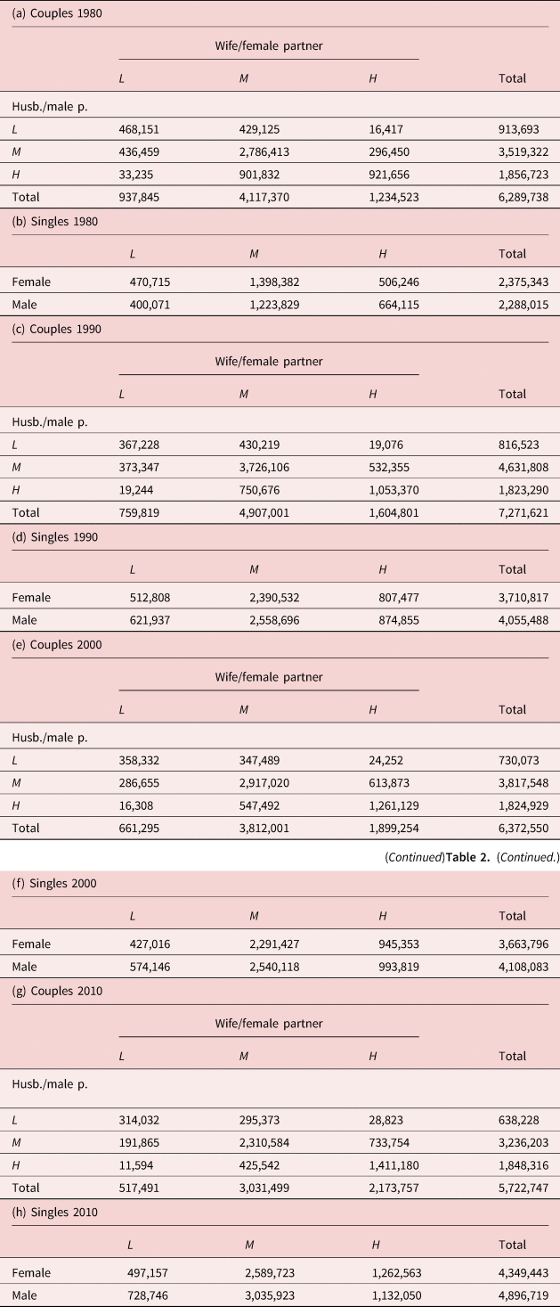
Source: Data are from the international version of Integrated Public Use Microdata Series (IPUMS) from the Minnesota Population Center.

Notes: Our sample covers heterosexual couples where the men are aged 30–34 years, and single people from the same age group. The variable on the highest level of education can take three different values, where L stands for “low level of education” corresponding to not having completed high school; M denotes “medium level of education” corresponding to having a high school degree; and H stands for “high level of education” corresponding to holding a university diploma.

Our sample covers those heterosexual young couples where the men are aged 30–34 years.Footnote ¹⁸ We do not distinguish between officially married couples and couples in a consensual union.Footnote ¹⁹ Hereafter, by “marriage” we mean both types of union.

In addition to couples, our data also cover single individuals from the same age group. Data on single people are used by the CS method, but not by the IPF algorithm and the new method.

Our variable on the highest level of education can take five values, i.e., “less than primary completed”, “primary completed”, “secondary completed”, “some college”, and “university completed”. For the main analysis, we merge the lowest two categories and also the next two categories. So, we work with the following three categories: “less than high school”, “high school completed”, and “university completed”.Footnote ²⁰

5.2. Stylized facts

Three stylized facts are documented by Tables 3 and 4. First, the studied period was characterized by an educational expansion. Second, the educational gender gap has closed and then it has reversed: in 2010, women in relationships with young men were more educated than their spouses on average, although it was just the opposite 30 years earlier. Third, the proportion of educationally homogamous couples has increased.

Table 3.

Educational distribution of married/in union young men and that of their spouses in the US between 1980 and 2010 (in %)

Source: Authors' calculations using data in Table 2.

Table 4.

The proportion of educationally homogamous couples in the US between 1980 and 2010 (in %)

Source: Authors' calculations using data in Table 2.

The first two stylized facts clearly show that the structural availability of marriageable men and women with a given qualification level has changed. Whether these changes can fully explain the observed increase in the prevalence of homogamy is undoubtedly an important empirical question.Footnote ²¹ An equally relevant and exciting question is whether the answer to the previous question depends on the choice of the method applied for the analysis. This is addressed in the next section.

5.3. The empirical application of the new method

Let us apply the methodology introduced in section 4 to the data described in subsection 5.1. It involves the following three steps. First, we construct the contingency tables under the counterfactuals. This is the step where we apply the new method introduced in subsection 4.2.2. Second, we calculate the share of educationally homogamous couples. For that, we simply take the sum of the diagonal elements in each of the observed contingency tables and divide it by the corresponding total number of couples. We obtain f(A ₁₉₈₀, P ₁₉₈₀), f(A ₁₉₉₀, P ₁₉₉₀), f(A ₂₀₀₀, P ₂₀₀₀), and f(A ₂₀₁₀, P ₂₀₁₀). Similarly, we calculate the share of educationally homogamous couples in each of the six counterfactual tables. We obtain f(A ₁₉₈₀, P ₁₉₉₀), f(A ₁₉₉₀, P ₁₉₈₀), f(A ₁₉₉₀, P ₂₀₀₀), f(A ₂₀₀₀, P ₁₉₉₀), f(A ₂₀₀₀, P ₂₀₁₀), f(A ₂₀₁₀, P ₂₀₀₀). Finally, we apply the decomposition scheme in equation (11) three times (or, equation (12)).

5.3.1. Results of the main analysis

Figure 1 presents the outcome of the main decomposition. It reports the extent to which certain drivers contributed to the changes in the share of educationally homogamous couples in the US between 1980 and 2010. Figure 1b shows the results for the investigated three decades separately, while these outcomes are aggregated in Figure 1a.

Figure 1.

The long-horizon and short-horizon decompositions of changing prevalence of marital homogamy in the US with counterfactuals constructed by three different methods.

Source: Authors' calculations using data in Table 2.

Notes: The decompositions are performed with the decomposition scheme in equation (11) for each of the three decades (1980–1990, 1990–2000, and 2000–2010), and with the three methods (Choo–Siow method, IPF algorithm, and the new method). The results are presented in 1b. The corresponding aggregate components obtained with the decomposition scheme in equation (12) are presented in 1a.

The results presented in Figure 1 cover not only the decompositions performed with the new method, but also those obtained with the CS solution, and the IPF algorithm.Footnote ²² Regarding some other methods, we cannot present decompositions with them. This is because the transformed contingency table has a negative cell when it is obtained with any of the statistical approaches, where the covariance, or the Pearson's correlation, or the regression coefficient is kept fixed.Footnote ²³

Figure 1a suggests that the components are robust to the choice of the method when the decomposition is applied to the period between 1980 and 2010.Footnote ²⁴ Interestingly, it is not the case with all the decade-specific components (see Figure 1b). For the period between 1980 and 1990, the sign of the decomposed effect of varying marital preferences across the groups of young American adults from different cohorts depends on whether the new method is applied or any of its alternatives. Footnote ²⁵ Whereas for the period between 2000 and 2010, it is the magnitude of the same effect that is sensitive to the choice of the method (see the dark bars of Figure 1b).

The analysis in this section had a limited scope in documenting differences between the empirical findings of the methods. The next subsection checks the robustness of some findings obtained with the new method. While in subsection 5.4, we use some survey evidence and the decade-specific components to support our claim that the new method is better than its two alternatives.

5.3.2. Robustness checks

In this subsection, we investigate whether our decompositions obtained with the new method are robust to some choices; specifically, the choice on the number of educational categories (3 in the main specification, 4 in its two alternatives), and the definition of young couples (men are aged 30–34 years vs. women are aged 30–34 years).

We present not only the decade-specific results (see Figure 2b), but also the aggregate results (see Figure 2a). However, we interpret only the decade-specific results since we use them for method selection. Lack of their robustness would undermine the concept of selection. Fortunately, this is not the case: Figure 2b shows that the sign of the decade-specific components is sensitive neither to the definition of young couples, nor to the educational categories considered. Moreover, the magnitude of the marital preference-component in the last decade is also robust (see the dark bars in Figure 2b belonging to the period 2000–2010).

Figure 2.

The long-horizon and short-horizon decompositions of changing prevalence of marital homogamy in the US with counterfactuals constructed by the new method.

Source: Authors' calculations using data in Table 2.

Notes: In the first case, we introduced the educational category “some college” by splitting the middle education category of the main analysis. In the second case, we introduced the education category “less than primary completed” by splitting the lowest category of the main analysis. In the third case, we defined young couples with the age of the wives/female partners by restricting it between 30 and 34 years. The decade-specific components in 2b are summed in order to obtain the results of the long-horizon decompositions reported in 2a. The decomposition scheme used is the same as in the main analysis.

5.4. A supplementary analysis

When different methods deliver contrasting results, it calls for checking how well these results fit other evidence. To study whether the CS solution, the IPF algorithm or the new method provides us with a more realistic view, we use survey evidence from the Pew Research Center on the views of different generations about spousal education.

The Changing American Family survey conducted in 2010 informs us about two shares: the share of men who say it is very important for a woman to be well-educated in order to be a good wife/partner; and the share of women who say it is very important for a man to be well-educated in order to be a good husband/partner.Footnote ²⁶ This survey is not designed to identify directly those respondents who have preferences for homogamy. Therefore, we cannot learn from it what share of the male and female respondents prefer to mate with others who have the same education level as they do.

Obviously, the observed shares and the shares that cannot be identified from the survey capture the prevalence of different types of preferences in society. However, as it is pointed out by Hitsch et al. (Reference Hitsch, Hortaçsu and Ariely2010) and others, “both types of preferences can lead to empirically observed assortative mating patterns [Becker (Reference Becker1973), Browning et al. (Reference Browning, Chiappori and Weiss2008), and Kalmijn (Reference Kalmijn1998)] and are thus indistinguishable using data on marriages only.” On the one hand, the point they make questions whether the effects identified in the previous section are really the effects of changing preferences for partners with the same education level or, rather, they are the effects of changing preferences for well-educated partners. On the other hand, their point motivates us to use the variation in the observed shares across generations as a proxy for the effect of changing marital preferences irrespective of the exact type of these preferences.

When analyzing the survey data, our primary focus is on the responses of the early baby boomers (who were in the age group of 30–34 in the census year 1980) and the late boomers (who were in the same age group 10 years later in 1990) since the conflicting findings presented in subsection 5.3 were related to the revealed preferences of these two generations.

Figure 3 shows that in 2010 spousal education was viewed to be very important by 35% of the women respondents and 34% of the men respondents among the late boomers. These shares are lower than the corresponding shares in the generation of early boomers (around 39% and 45%, respectively). The detected variation across generations suggests that the changing composition of the studied age group with respect to its members' marital/mating preferences has a negative effect on the share of educationally homogamous young couples in the US between 1980 and 1990. The latter finding is in line with the result obtained by the new method, but not with those of the CS method and the IPF algorithm (see the dark bars in Figure 1b for the period 1980–1990).

Figure 3.

Generation-specific views from the opposite sex on the importance of spousal education in the US in 2010.

Source: Authors' calculations based on the answers to the survey questions number 23 and number 24 in the Changing American Family survey conducted by the Pew Research Center in 2010.

Notes: Answering the corresponding survey questions was refused by 3 women (aged 35, 55, and 87 in 2010) and 1 men (aged 57 in 2010), while the questions were answered by 289 women and 237 men in the age groups studied. Out of the 289 women 84 were in the age group 60–64 (representing early boomers), 92 were in the age group 50–54 (representing late boomers), 60 were in the age group 40–44 (representing early generation-X) and 53 were in the age group 30–34 (representing late generation-X) in 2010. Out of the 237 men respondents 56 were in the age group 60–64, 75 were in the age group 50–54, 61 were in the age group 40–44, 45 were in the age group 30–34 in the same year. The 95% symmetric confidence intervals are obtained with the approximation proposed by Agresti and Coull (Reference Agresti and Coull1998).

Moreover, Figure 3 shows that there is a remarkable difference not only between the early boomers and the late boomers but also between the early generation-X (who were in the age group of 30–34 in 2000) and the late generation-X (who were in the same age group in 2010) regarding their preferences. In 2010, spousal education was viewed to be very important by about 41% of the female and 32% of the male respondents in the early generation-X. These shares are higher in the late generation-X since those are close to 46% and 45%, respectively. This survey evidence suggests that the share of educationally homogamous young couples would have increased massively between 2000 and 2010 if the educational composition of the early generation-X and that of the late generation-X had been the same. This result is again more in line with the finding obtained by the new method than with the finding obtained with its alternatives (see the dark bars of Figure 1b for the period 2000–2010).

All in all, the reviewed survey evidence yield support for the new method.Footnote ²⁷