

1. Introduction
With the development of molecular markers, quantitative trait locus (QTL) mapping has become a routine approach for genetic studies of complex traits in plants, animals and humans, where the construction of linkage maps is a crucial step (Wu et al., Reference Wu, Han, Hu, Fang, Li, Li and Zeng2000). To construct an accurate linkage map, precisely estimating recombination frequency is the key and this has been widely studied over many years (Fisher, Reference Fisher1935; Haldane & Smith, Reference Haldane and Smith1947; Morton, Reference Morton1955; Smith, Reference Smith1953, Reference Smith1959; Ott, Reference Ott1974; Nordheim et al., Reference Nordheim, O'Malley and Guries1983; Ritter et al., Reference Ritter, Gebhardt and Salamini1990; Frisch & Melchinger, Reference Frisch and Melchinger2007). In addition to linkage maps construction, recombination frequency needs to be precisely estimated for QTL fine mapping, marker-assisted backcrossing, marker-assisted selection, map-based cloning, etc.
Many factors may affect the accuracy of recombination frequency estimation. Säll & Nilsson (Reference Säll and Nilsson1994) investigated the accuracy of recombination frequency estimates with respect to (1) limited sample size, (2) heterogeneity in recombination frequency between sexes or among meioses and (3) factors that distort the segregation misclassification or differential viability. Xu & Zhou (Reference Xu and Zhou2000) showed that linkage analysis was more reliable if the real recombination frequency between two loci was less than or equal to 0·15 when population size (PS) was 50. Hackett & Broadfoot (Reference Hackett and Broadfoot2003) demonstrated that missing values and/or typing errors in genotyping reduced the proportion of correctly ordered maps, and the presence of segregation distortion had little effect on marker order in the linkage maps. Frisch & Melchinger (Reference Frisch and Melchinger2007) investigated the effect of mating scheme on the precision of recombination frequency estimates.
Various types of population have been used to estimate the recombination frequency and then to construct linkage maps. For examples, types of populations in rice include F2 (Harushima et al., Reference Harushima, Yano, Shomura, Sato, Shimano, Kuboki, Yamamoto, Lin, Antonio and Parco1998), doubled haploids (DH; Temnykh et al., Reference Temnykh, DeClerck, Lukashova, Lipovich, Cartinhour and McCouch2001), recombination inbred lines (RIL; Sirithunya et al., Reference Sirithunya, Tragoonrung, Vanavichit, Pa-In, Vongsaprom and Toojinda2002), backcross (BC1F1; Yan et al., Reference Yan, Liang, Chen, Li, Tang, Yi, Tian, Lu and Gu2003), advanced backcross (BC3F1; Tan et al., Reference Tan, Zhang, Liu, Wang, Ye, Zhu, Fu, Cai and Sun2008) populations, etc. In soybean, BC1F1 (Lu et al., Reference Lu, Gai, Zheng and Li2006), BC1F3 (Li et al., Reference Li, Jiang, Zhang, Qiu, Liu, Li, Gao, Chen and Hu2008), RIL (Liu et al., Reference Liu, Zhou, Yu, Chen and Gai2009), F2 (Wang et al., Reference Wang, Xu, Li, Li, Gen and Zhang2010), etc. have been used to construct linkage maps. One commonly observed problem is different populations result in inconsistent linkage maps even if the same set of markers was used in genotyping (Liang et al., Reference Liang, Peng, Ye, Li, Sun, Ma and Li2007). Antonio et al. (Reference Antonio, Inoue, Kajiya, Nagamura, Kurata, Minobe, Yano, Nakagahra and Sasaki1996) compared genetic distance and the order of DNA markers in five populations of rice. The five populations consisted of three F2, one BC1F1 and one RIL, which were derived from different parents. They concluded that about 170 DNA markers commonly mapped in the five populations showed the same linkage groups with conserved linkage order. However, the genetic distances between markers among the five populations were not completely consistent due to the differences in genetic backgrounds. Liang et al. (Reference Liang, Peng, Ye, Li, Sun, Ma and Li2007) found that the linkage maps of F2 and F6 populations derived from the same rice subspecies cross differed in linkage groups, linked markers, genetic orders and genetic distances.
It would be useful to know which populations were more suitable for estimating recombination frequency in order to guarantee the high efficiency of linkage analysis. Our objectives in this study were to investigate the effect of population type and size on the estimation of recombination frequency and then to determine the most suitable bi-parental populations to estimate the recombination frequency.
2. Materials and methods
(i) Bi-parental populations in plant genetics and breeding
Populations commonly used in plant genetics and breeding are shown in Fig. 1, which were derived from two homozygous parental lines P1 and P2. Backcross populations when P1 was used as the recurrent parent had the same genetic structure as those when P2 was used as the recurrent parent. Therefore, when P1 was used as the recurrent parent only backcross populations were considered, i.e. 12 bi-parental populations were used to compare the precision of recombination frequency estimates in this study.
Bi-parental populations commonly used in genetic studies of plants.

According to the frequency of P1 alleles, these populations can be roughly classified as F1-derived where the P1 allele frequency was 0·5 (i.e. F2, F3, F1DH and F1RIL), BC1F1 and BC1F1-derived where the P1 allele frequency was 0·75 (i.e. BC1F1, BC1F2, BC1DH and BC1RIL), and BC2F1 and BC2F1-derived where the P1 allele frequency was 0·875 (i.e. BC2F1, BC2F2, BC2DH and BC2RIL). Relationship among the 12 bi-parental populations is shown in Fig. 1.
(ii) Theoretical frequencies of genotypes at two linked loci
Assuming that A/a and B/b were two linked marker loci in a diploid species, and the recombination frequency per meiosis was denoted as r. In the F1RIL population which was derived from repeated selfing since F1, recombination frequency was denoted as r RIL. The relationship between r RIL and r at two linked loci was r RIL=2r/(1+2r) (Haldane & Waddington, Reference Haldane and Waddington1931). Assuming two markers were co-dominant, frequencies of possible genotypes in each population could be expressed by r and r RIL (Table 1). Double heterozygous was distinct as AB/ab for the coupling linkage and Ab/aB for the repulsion linkage. In this sense, genotypes in F1 population were AB/ab. Assuming that there is no extensive selection affecting marker-allele frequencies, the frequencies of their four gametes AB, Ab, aB and ab were (1−r)/2, r/2, r/2 and (1−r)/2, respectively. Assuming independence of meiotic behaviour from generation, genotypic frequencies of BC1F1 and BC2F1 populations can be calculated from the genotypic frequency of F1 population through backcross transition matrix (Nelson, Reference Nelson2011). Through selfing transition matrix (Nelson, Reference Nelson2011), genotypic frequencies of F2 and F3 populations can be calculated from the genotypic frequency of F1 population, and genotypic frequencies of BC1F2 and BC2F2 populations can be calculated from the genotypic frequencies of BC1F1 and BC2F1 populations, respectively. Through DH-transition matrix (Nelson, Reference Nelson2011), genotypic frequencies of F1DH population can be calculated from the genotypic frequency of F1 population, and genotypic frequencies of BC1DH and BC2DH populations can be calculated from the genotypic frequencies of BC1F1 and BC2F1 populations, respectively. The genotypic frequencies of F1RIL, BC1RIL and BC2RIL were similar to those of F1DH, BC1DH and BC2DH, except that r was replaced by r RIL since the repeated selfing.
Genotypic frequencies for 12 bi-parental populations when alleles A and a are co-dominant at marker locus A/a and alleles B and b are co-dominant at marker locus B/b
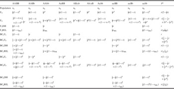
a The frequency of recombinant zygotes, blanks stand for zero, and r RIL=2r/1+2r.
It should be noted that four genotypic frequencies of BC1F1 and BC2F1 were the same as those of F1DH and BC1DH, respectively (Table 1). Genotypic frequencies in F1RIL and BC1RIL were similar to those of the corresponding backcross (BC1F1 and BC2F1) and DH (F1DH and BC1DH) populations, respectively, except that r was substituted by −r RIL. Due to the backcross, frequencies of parental genotype and recombinant genotype were not balanced, especially after two rounds of backcrossing. For two co-dominant loci, there were 10 genotypes for F2, BC1F2, BC2F2 and F3 populations, due to the coupling and repulsive linkage for double heterozygous, and four genotypes for the other eight populations (Table 1).
When marker loci A/a and B/b were not both co-dominant, frequencies of possible genotypes in populations BC1F1, F2, F3, BC2F1, BC1F2 and BC2F2 (Tables S1–S5 available online at http://journals.cambridge.org/GRH) could be derived by using the frequencies in Table 1. Co-dominant marker was denoted by C, dominant marker was denoted by D and recessive marker was denoted by R in Tables S1–S5. Six cases were considered including (C, C), (C, D), (C, R), (D, D), (D, R) and (R, R). (D, C), (R, C) and (R, D) were not considered, since the same results would be retained as (C, D), (C, R) and (D, R), respectively. When allele A is dominant to allele a in marker locus A/a, no polymorphism at locus A/a for populations BC1F1 and BC2F1. Hence, BC1F1 and BC2F1 were not considered in (C, D) (Table S1), (D, D) (Table S3) and (D, R) (Table S4).
(iii) Estimation of recombination frequency
The maximum likelihood (ML) method was used to estimate recombination frequency (Fisher, Reference Fisher1935; Bailey, Reference Bailey1961; Wu et al., Reference Wu, Ma and Casella2007). For any type of population, there are K observed genotype categories (K=10 in Table 1; K=6 in Tables S1 and S2; and K=4 in Tables S3–S5). For each observed genotype, a probability can be derived, which is a function of r. This probability is denoted by pk
(r) for the kth observed genotype. Let nk
be the observed count for the kth genotype, then the multinomial log-likelihood function is, ![]() . To obtain the ML solution of r, we need to differentiate L(r) with respect to r and set the derivative equal to zero, i.e. L′(r)=0. It was difficult to obtain the analytic estimate of r due to the complexity of L′(r)=0. However, it was feasible to have the numerical solutions by applying the Newton–Raphson algorithm.
. To obtain the ML solution of r, we need to differentiate L(r) with respect to r and set the derivative equal to zero, i.e. L′(r)=0. It was difficult to obtain the analytic estimate of r due to the complexity of L′(r)=0. However, it was feasible to have the numerical solutions by applying the Newton–Raphson algorithm.
The Newton–Raphson algorithm for the ML solution of r is
where L′(r) and L″(r) are the first- and second-order derivatives of the log-likelihood function with respect to r, respectively. Assuming that the iteration process converges when t=T, the maximum likelihood estimation (MLE) of r is ![]() .
.
The variance of the estimated r is approximated by ![]() , where
, where ![]() is the second derivative of the log-likelihood function with respect to r, evaluated at
is the second derivative of the log-likelihood function with respect to r, evaluated at ![]() , and
, and ![]() is the expectation of
is the expectation of ![]() with respect to nk
(see supplementary material).
with respect to nk
(see supplementary material).
(iv) Test of the linkage relationship between two loci
The existence of the linkage can be tested by the following hypotheses:
where H
0 is the null hypothesis, corresponding to no linkage; H
A is the alternative hypothesis, corresponding to the genetic linkage between the two loci; and ![]() is the estimated recombination frequency. The log-likelihood function under the null hypothesis is L
0=log[L(r=0·5)], whereas the log-likelihood function under the alternative hypothesis is
is the estimated recombination frequency. The log-likelihood function under the null hypothesis is L
0=log[L(r=0·5)], whereas the log-likelihood function under the alternative hypothesis is ![]() . The LOD score can be calculated from the log-likelihoods under the two hypotheses, i.e. L
A
−L
0.
. The LOD score can be calculated from the log-likelihoods under the two hypotheses, i.e. L
A
−L
0.
(v) The least PS to observe one recombinant
To facilitate our demonstration, the frequencies of each genotype in Table 1 and Tables S1–S5 were denoted as f
1, f
2, …, fK
, and the probabilities of K genotypes to have recombinants observed were denoted as p
1, p
2, …, pK
(K=10 in Table 1; K=6 in Tables S1 and S2; and K=4 in Tables S3–S5). Thus (p
1, p
2, p
3, p
4, p
5, p
6, p
7, p
8, p
9, p
10)=(0, 1, 1, 1, 0, 0, 1, 1, 1, 0) in Table 1, (p
1, p
2, p
3, p
4, p
5, p
6)=(0, 1, 0, 1, 1, 0) in Table S1, (p
1, p
2, p
3, p
4, p
5, p
6)=(0, 1, 1, 0, 1, 0) in Table S2, (p
1, p
2, p
3, p
4)=(0, 1, 1, 0) in Tables S3 and S5, and (p
1, p
2, p
3, p
4)=(0, 0, 1, 0) in Table S4. Therefore, the probability of a population to have at least one recombinant observed would be ![]() . The recombinant probability (p) of each bi-parental population is shown in Table 1 and Tables S1–S5 as well. The theoretical PS required to observe at least one recombinant at the 95% confidence level could be calculated from the equation (1−p)
n
=0·05, i.e. n=ln(0·05)/ln(1−p).
. The recombinant probability (p) of each bi-parental population is shown in Table 1 and Tables S1–S5 as well. The theoretical PS required to observe at least one recombinant at the 95% confidence level could be calculated from the equation (1−p)
n
=0·05, i.e. n=ln(0·05)/ln(1−p).
(vi) The least PS to declare a significant linkage relationship
With a given PS, say n, and given r, the expected observation of each genotype is equal to nk =fkn, where fk (k=1, …, K; K=10 in Table 1; K=6 in Tables S1 and S2; and K=4 in Tables S3–S5) is the frequency of each genotype in Table 1 and Tables S1–S5. The theoretical log-likelihood function under the alternative hypothesis is L A(r, n)=log[L(r, nk ; k=1, …, K)], and the log-likelihood function under the null hypothesis is L 0=log[L(r=0·5)]. Therefore, the theoretical LOD score for given r and n, is L A(r, n)−L 0. For a given r and PS n, the expected LOD score can be calculated, where the least PS to test linkage, that is LOD⩾3, can be determined.
(vii) Simulation of the bi-parental genetic populations
The simulated genome consisted of seven chromosomes, each with two linked markers. Only co-dominant markers were considered in simulation. The recombination frequencies between each marker pair were 0·01, 0·02, 0·03, 0·05, 0·10, 0·20 and 0·30, respectively, which were converted to marker distance by Haldane mapping function when conducting the simulation experiments. A thousand replications of each of the 12 bi-parental populations were simulated under five levels of size (PS=50, 100, 200, 300 and 500). Simulated populations were generated by the integrated software for building linkage maps and mapping QTL, which is called QTL IciMapping (available from http://www.isbreeding.net). The LOD score and estimated recombination frequency were calculated by averaging the 1000 simulated runs.
3. Results
(i) Comparison of LOD score in testing the linkage relationship
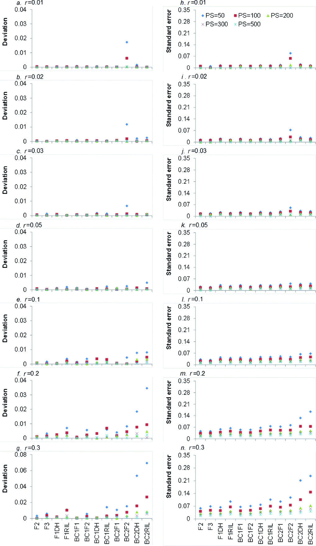
LOD score is the test statistic for detecting the significance of recombination frequency (r) compared with independent inheritance. When LOD score is greater than a threshold value (generally 3), the two loci under consideration are declared to be linked; otherwise they are independent. The higher the LOD score, the more significant is the linkage between the two loci. Averaged LOD scores and their respective standard errors (SEs) of 12 bi-parental genetic populations under five levels of PS and seven levels of r are showed in Fig. 2.
Average LOD scores (a–g) and their respective SEs (h–n) from 1000 simulations in 12 bi-parental populations corresponding to seven levels of recombination frequencies (r=0·01, 0·02, 0·03, 0·05, 0·1, 0·2 and 0·3) and five PS (PS=50, 100, 200, 300 and 500). Only co-dominant markers were considered.

It is clear that larger PS and smaller r resulted in higher LOD score, regardless of the population type (Fig. 2 a–g). For each population type, LOD score reached the highest when PS=500, but it declined sharply when r=0·1. This indicated that large PS and small r were favourable to detect the linked markers. LOD scores of the 12 bi-parental populations were significantly different (Fig. 2 a–g), but similar trend can be seen for different r and PS values. LOD scores of four F1-derived populations (i.e. F2, F3, F1DH and F1RIL) were higher than those of BC1F1 and three BC1F1-derived populations (i.e. BC1F2, BC1DH and BC1RIL), respectively. BC1F1 and three BC1F1-derived populations have higher LOD scores than BC2F1 and three BC2F1-derived populations (i.e. BC2F2, BC2DH and BC2RIL), respectively. That is to say, LOD scores declined with the round of backcrossing. Taking r=0·01 and PS=300 for an example (Fig. 2 a), LOD score of BC2DH was lower than that of BC1DH. LOD score of F1DH was the highest among DH populations (i.e. F1DH, BC1DH and BC2DH). The reason is that backcrossing makes the allele frequency in one locus be apart from 0·5, which is detrimental for recombination frequency estimation. LOD scores of BC1F1 and BC2F1 were similar to those of F1DH and BC1DH, respectively, due to the same genotypic frequencies (Table 1).
LOD scores of three RILs populations (i.e. F1RIL, BC1RIL and BC2RIL) were lower than those of corresponding backcross (BC1F1 and BC2F1) and DH (F1DH, BC1DH and BC2DH) populations, since the recombination frequency caused by meiosis in multiple generations (−r RIL) was greater than that by meiosis in one generation (r). LOD scores of F2 and F2-related populations (i.e. F3, BC1F2 and BC2F2) were higher than those of the corresponding backcross (i.e. BC1F1 and BC2F1), DH (i.e. F1DH, BC1DH and BC2DH) and recombinant inbred lines (i.e. F1RIL, BC1RIL and BC2RIL). The possible reason is that F2 and F2-related populations had 10 genotypes, whereas other populations had only four genotypes (Table 1), and more genotypes might provide more recombination information. In most cases, LOD scores of F2 population were the highest, except when r=0·01, PS=100–500 (Fig. 2 a) and r=0·02, PS=500 (Fig. 2 b) where LOD scores of F3 population were the highest.
Higher PS resulted in higher SE of LOD scores, which was similar to the trend of LOD score (Fig. 2 h–n). For the increased rounds of backcrossing and r, SE was generally decreased, due to the decreased LOD score. However, when r⩽0·05 the SE of LOD scores slightly increased as the round of backcrossing and r increased (Fig. 2 h–k). The SE of F2 population slightly increased from 6·767 (r=0·01) to 8·408 (r=0·05), and then decreased to 4·018 (r=0·3).
(ii) Comparison of accuracy in estimating recombination frequency
Absolute deviation between estimated and real recombination frequencies and their respective SE under seven levels of r and five levels of PS are shown in Fig. 3. Small deviation and SE implied accurate recombination frequency estimation. As expected, the deviation and SE of estimated recombination frequency decreased with the increase of PS. When PS⩾200 the deviation and SE for the 12 populations were almost equal to zero. It indicated that increasing sample sizes always led to high precision of estimation. Generally, the deviations became large with the increase of r (Fig. 3 e–g). For r=0·01, the deviations were close to zero except for those under BC2F2 population (Fig. 3 a). When r increased, the deviations became significantly large (Fig. 3 e–g). In terms of the population type, deviations for F2 population were almost equal to zero regardless of PS and r. The deviations of BC2F1-related populations (i.e. BC2F1, BC2DH, BC2RIL and BC2F2) were generally higher than those of other eight populations (Fig. 3 a–g), which indicated that more rounds of backcrossing were not favoured for precision estimation of recombination frequency. SE of estimated recombination frequencies increased with the increase of r and rounds of backcrossing, which were similar to the trends in deviations (Fig. 3 h–n). Among the 12 populations, SE of F2 population was generally the smallest.
Average deviations between estimated recombination frequencies and real recombination frequencies (a–g) and SEs of estimating recombination frequencies (h–n) from 1000 simulations in 12 bi-parental populations corresponding to seven levels of recombination frequencies (r=0·01, 0·02,0·03, 0·05, 0·1, 0·2 and 0·3) and five PS (PS=50, 100, 200, 300 and 500). Only co-dominant markers were considered.
To further investigate the effect of population type on the precision of recombination frequency estimation, we compared the theoretical SE under seven levels of r and PS=50 in 12 bi-parental populations (Table 2). The theoretical SE were calculated from second derivative of the log-likelihood function ![]() (for details, see Materials and methods section) that is
(for details, see Materials and methods section) that is ![]() , where
, where ![]() is the estimate of r and n is the sample size. The theoretical SE when two markers were co-dominant were consistent with the averaged SE obtained from 1000 simulation runs, due to the large sample property of population mean (Table 2 and Fig. 3). The theoretical SE increased with the increase in r and rounds of backcrossing (Table 2), which was consistent with what we had seen in the simulated results (Fig. 3). SE of BC1F1 and BC2F1 were equal to those of F1DH and BC1DH (Table 2 and Fig. 3), respectively, due to the same genotypic frequencies when two markers were co-dominant (Table 1). The theoretical SE of BC2RIL was the highest among the 12 populations regardless of the level of r. When r⩽0·1 the theoretical SE of F3 was the lowest, whereas when r>0·1 those of F2 was the lowest.
is the estimate of r and n is the sample size. The theoretical SE when two markers were co-dominant were consistent with the averaged SE obtained from 1000 simulation runs, due to the large sample property of population mean (Table 2 and Fig. 3). The theoretical SE increased with the increase in r and rounds of backcrossing (Table 2), which was consistent with what we had seen in the simulated results (Fig. 3). SE of BC1F1 and BC2F1 were equal to those of F1DH and BC1DH (Table 2 and Fig. 3), respectively, due to the same genotypic frequencies when two markers were co-dominant (Table 1). The theoretical SE of BC2RIL was the highest among the 12 populations regardless of the level of r. When r⩽0·1 the theoretical SE of F3 was the lowest, whereas when r>0·1 those of F2 was the lowest.
Theoretical SEs under seven levels of recombination frequency in 12 bi-parental populations when PS=50

a Assuming A and a are the two marker alleles at one locus, B and b are the two marker alleles at the other locus. (C, C) denotes that A and a are co-dominant, and B and b are co-dominant; (C, D) denotes that A and a are co-dominant, and B is dominant to b; (C, R) denotes that A and a are co-dominant, and B is recessive to b; (D, D) denotes that A is dominant to a, and B is dominant to b; (D, R) denotes that A is dominant to a, and B is recessive to b; and (R, R) denotes that A is recessive to a, and B is recessive to b.
To evaluate the effect of dominant and recessive markers on the estimation of recombination frequency, we considered dominant and recessive markers in populations F2, F3, BC1F1, BC1F2, BC2F1 and BC2F2. Generally, theoretical SE increased when markers were dominant and/or recessive, since fewer genotypes were observed (Tables S1–S5). The advantage of using co-dominant markers became obvious when r was getting large. SEs under (D, R) were the largest (Table 2) among the six cases (C, C), (C, D), (C, R), (D, D), (D, R) and (R, R) for populations F2, F3, BC2F1 and BC2F2. The reason is that only one recombinant genotype can be observed under (D, R), whereas in the other three genotype groups we cannot distinguish recombinant and non-recombinant from observations (Table S4).
(iii) PS required to observe at least one recombinant and to declare the significant linkage relationship
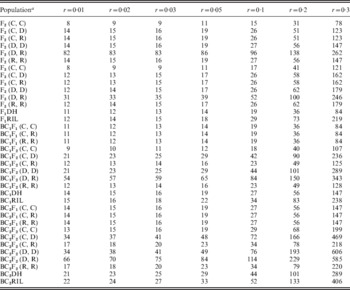
To detect the linkage between two loci, we need the PS to be large enough to guarantee that (1) at least one recombinant can be observed for tight linkage (Table 3) and (2) LOD score is greater than a threshold of 3 for loose linkage (Table 4). Small r implied a tight linkage between two loci. From the results in previous sections, LOD score for tight linkage was always high, which indicated that there was more chance to detect linkage, while recombinant was difficult to occur. In this sense, for a specific population type with r increased, PS required to make at least one recombinant observed decreased sharply (Table 3), while to make the linkage statistically significant increased conspicuously (Table 4). Therefore, the maximum value of the two PS in Tables 3 and 4 should be used in the application. Taking BC1F1 under two co-dominant markers for example, we needed 299 individuals to be 95% sure to observe at least one recombinant for r=0·01, while 11 individuals were enough to make it statistically significant. Therefore, when we develop a BC1F1 for linkage analysis, at least 299 individuals should be included.
Theoretical PS required to have at least one recombinant observed under 95% confidence level for seven levels of recombination frequencies in 12 bi-parental populations

a Assuming A and a are the two marker alleles at one locus, B and b are the two marker alleles at the other locus. (C, C) denotes that A and a are co-dominant, and B and b are co-dominant; (C, D) denotes that A and a are co-dominant, and B is dominant to b; (C, R) denotes that A and a are co-dominant, and B is recessive to b; (D, D) denotes that A is dominant to a, and B is dominant to b; (D, R) denotes that A is dominant to a, and B is recessive to b; and (R, R) denotes that A is recessive to a, and B is recessive to b.
Theoretical PS required to detect linkage between two loci (LOD⩾3) for seven levels of recombination frequencies in 12 bi-parental populations
a Assuming A and a are the two marker alleles at one locus, B and b are the two marker alleles at the other locus. (C, C) denotes that A and a are co-dominant, and B and b are co-dominant; (C, D) denotes that A and a are co-dominant, and B is dominant to b; (C, R) denotes that A and a are co-dominant, and B is recessive to b; (D, D) denotes that A is dominant to a, and B is dominant to b; (D, R) denotes that A is dominant to a, and B is recessive to b; and (R, R) denotes that A is recessive to a, and B is recessive to b.
For a specific level of r, the least PS required for observing at least one recombinant and to detect the linkage for BC2F1-derived populations was always large. Taking r=0·03 and case (C, C) as an example, the least PS required to observe at least one recombinant was 136 for BC2DH (Table 3), which was the largest among the 12 populations if markers were co-dominant. The least PS required to detect the linkage was 27 for BC2RIL (Table 4), which was the largest among the 12 populations. The results indicated that more rounds of backcrossing were not favoured in linkage analysis.
In terms of marker type, similar trends can be seen in Tables 3 and 4 as those in Table 2. The least PS required to observe one recombinant and to detect linkage increased when dominant and recessive markers were considered, especially when r is large. Under (D, R), a huge population was needed to observe one recombinant and to detect linkage (Tables 3 and 4). The required PS for F2 and F3 populations under (C, C) (Tables 3 and 4) was always the smallest regardless of the level of r, which showed the advantages of using F2 and F3 to estimate the recombination frequency for co-dominant markers.
Furthermore, we calculated the ratios (p/r) of the frequency of recombinant zygotes (p; Table 1 and Tables S1–S5) and recombination frequency (r) for two linked loci. p/r>1 implies that r was magnified by the estimated proportion of recombinant zygotes in the corresponding population; p/r=1 implies that r was unbiased by the estimated proportion of recombinant zygotes in the corresponding population; and p/r<1 implies that r was reduced by the estimated proportion of recombinant zygotes in the corresponding population. When r was magnified, it will be easy to observe the recombinant, and detect the linkage. p/r under two co-dominant markers are shown in Fig. 4. p/r decreased, while all were greater than 1 under populations F3, F2, F1RIL, BC1F2, BC1RIL and BC2F2. Thus, the power to estimate r was high, and small samples were needed to observe recombinant and detect the linkage in those populations, especially in F3 population, which were consistent with the results we have seen in Fig. 2, and Tables 3 and 4. p/r<1 under populations BC1DH, BC2F1, BC2RIL and BC2DH, which indicated that these four populations were inappropriate to estimate r. p/r under BC2F1-derived populations were smaller than those under F1-derived populations and BC1F1-derived populations, which indicated the inferior r estimation from two rounds of backcrossing populations once again. On the other hand, p/r was high when r was small, say r<0·1, which was consistent with the results in Fig. 2, and Tables 3 and 4. The advantage of using F3 population was weakened to that of F2 population when r>0·25.
Ratio (p/r) of the frequency of recombinant zygotes (p) and the recombination frequency (r) of two linked co-dominant marker loci. In addition to the 12 bi-parental populations described in Fig. 1, F4, BC1F3 and BC2F3 were included to evaluate the trend of p/r for repeated selfing.
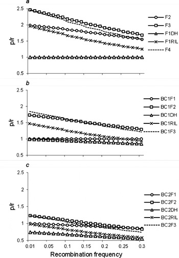
It should be noted that p/r under F2 populations across different r was higher than those under RIL population, but lower than those under F3 population (Fig. 4). In addition to the 12 bi-parental populations described in Fig. 1, one more selfing pollination after F3 (i.e. F4), BC1F2 (i.e. BC1F3) and BC2F2 (i.e. BC2F3) were included to evaluate the trend of p/r for repeated selfing. It turns out that from F4, BC1F3 and BC2F3 populations, p/r became lower and lower, and approached RIL, BC1RIL and BC2RIL populations, respectively, which indicated the less efficiency of advanced selfing populations in estimating recombination frequency.
4. Discussion and conclusion
Linkage analysis is fundamental in genetic studies. An accurate estimation of recombination frequency is essential for gene mapping, marker-assisted selection, map-based cloning, etc. Bi-parental populations have been widely used to estimate the recombination frequency in the application, but few studies can be identified in which populations were more suitable for estimating recombination frequency. In this study, 12 bi-parental populations were considered to investigate the efficiency in estimating the recombination frequency in theory and by extensive simulations. Actually, those 12 populations included most of the commonly used mating schemes of bi-parental populations in genetics and breeding.
Regarding the detection power, we compared the LOD scores under five levels of PS and seven levels of recombination frequency across 12 bi-parental populations. In terms of estimation precision, we compared deviations between estimated and real recombination frequencies under five PS, and the theoretical SEs under seven levels of recombination frequency across 12 bi-parental populations. Theoretically, we evaluated the least PS needed to observe at least one recombinant and to make the linkage detected (i.e. LOD score was not less than 3) for co-dominant, dominant and recessive markers. In summary, detection power and estimation precision of two tightly linked loci (i.e. small recombination frequency) were high. Large size of population is critical for recombination frequency estimation. Advanced backcrossing and selfing populations reduce the precision in estimating the recombination frequency. For dominant and recessive markers, large-sized populations were needed to observe at least one recombinant and detect the genetic linkage, indicating that dominant and recessive markers should be avoided as much as possible in recombination frequency estimation. For the 12 populations considered in this study, F2 and F3 populations with co-dominant markers had the highest power and precision to estimate the recombination frequency.
For co-dominant markers, F2 and F3 populations showed advantages over backcross (i.e. BC1F1 and BC2F1), DH (i.e. F1DH, BC1DH and BC2DH) and recombinant inbred lines (i.e. F1RIL, BC1RIL and BC2RIL) (Figs. 2–4) on recombination frequency estimation. F2 and F3 populations had 10 genotypes, whereas backcross, DH and recombinant inbred lines had only four genotypes and no heterozygous (Table 1). For F2 and F3 populations, the theoretical standard deviations of estimated recombination frequency (Table 2), and the least PS needed to observe at least one recombinant (Table 3) and to make the linkage detected (Table 4) for co-dominant markers were smaller than those for dominant and recessive markers. Compared with co-dominant marker, using dominant and recessive markers merged some genotypes together, and cannot distinguish recombinant and non-recombinant from observations in some cases, which decreased the efficiency in recombination frequency estimation (Tables S1–S5). For example, for F2 and F3 populations under (C, C) (Table 1), there were 10 genotypes where AABb, AAbb, AaBB, Aabb, aaBB and aaBb were observed recombinant, and under (D, R) (Table S4) there were four genotypes where only aaBB can be observed as recombinant. Therefore, F2 and F3 populations with co-dominant markers have more genotypes than those with dominant and recessive markers, and those under backcross, DH and recombinant inbred lines.
For BC1F1 and BC2F1 the number of genotype using co-dominant markers (i.e. (C, C); Table 1) was the same as that using dominant and recessive markers (Tables S2 and S5). The theoretical least PS needed to observe at least one recombinant (Table 3) and to make the linkage detected were the same under (C, C), (C, R) and (R, R). It implied that marker type did not play an effect on recombination frequency estimation (Tables 3 and 4) for backcross populations. However, backcrossing made the allele frequency in one locus apart from 0·5, thus genotypic frequency among each genotype was greatly different, especially for multiple rounds of backcrossing. This difference was detrimental for recombination frequency estimation as well (Figs. 2–4 and Tables 2–4). Taking r=0·01 for example, the theoretical SE for the estimates of recombination frequency for F2, BC1F2 and BC2F2 populations using co-dominant markers were 0·0100, 0·0107 and 0·0127, respectively (Table 2). The theoretical PS required to have at least one recombinant observed for F2, BC1F2 and BC2F2 populations using co-dominant markers were 150, 172 and 242, respectively (Table 3). The theoretical PS required for detecting linkage for F2, BC1F2 and BC2F2 populations using co-dominant markers were 8, 9, and 13, respectively (Table 4).
Few advantages for advanced selfing populations to estimate recombination frequency were observed (Figs 2–4 and Tables 2–4). Taking r=0·01 for example, the theoretical SE for the estimates of recombination frequency for F2 and F1RIL, and BC1F2 and BC1RIL populations using co-dominant markers were 0·0100 and 0·0102, and 0·0107 and 0·0118, respectively (Table 2). The theoretical PS is required to have at least one recombinant observed for F2 and F1RIL, and BC1F2 and BC1RIL populations using co-dominant markers were 150 and 152, and 172 and 203, respectively (Table 3). The theoretical PS required to detect linkage for F2 and F1RIL, and BC1F2, and BC1RIL populations using co-dominant markers were 8 and 12, and 9 and 15, respectively (Table 4). Therefore, the advanced backcrossing and selfing populations were less efficient to estimate recombination frequency than backcross and F2 populations, respectively. Consequently, for a given PS F2 and F3 populations with co-dominant markers would have more information on recombination, and represent the ideal situation for recombination frequency estimation.
Bi-parental populations derived by random intermating from F2 generation, such as advanced intercross line (AIL; Darvasi & Soller, Reference Darvasi and Soller1995) and Intermated B73×Mo17 (IBM; Lee et al., Reference Lee, Sharopova, Beavis, Grant, Katt, Blair and Halauer2002) population, were not considered in this study. However, the basic principles and conclusions shown in this paper should apply to these populations as well. Continued intercrossing of a population would reduce linkage disequilibrium and cause the proportion of recombinants between any linked loci to asymptotically approach 0·5. Beavis et al. (Reference Beavis, Lee, Grant, Hallauer, Owens, Katt and Blair1992) showed that the recombination on chromosome 1 in maize, a 2·7-fold increase in the recombination frequency was observed in the IBM population after five generations of intermating. The expected recombination frequencies after t generations of random mating were calculated as r (t)=r (t−1)+[r (t−1)−2r2 (t−1)]/2, where r (t) is the frequency of recombinants after t generations of random mating and r (t−1) is the frequency of recombinants in the prior generation (Beavis et al., Reference Beavis, Lee, Grant, Hallauer, Owens, Katt and Blair1992). Genotypic frequencies in AIL or IBM population can be determined by random mating transition matrix (Falconer & Mackay, Reference Falconer and Mackay1996). Therefore, similar strategies as those used in this study can be utilized to evaluate the efficiency of AIL and IBM populations on recombination frequency estimation.
In this study, we evaluated the efficiency of 12 bi-parental populations to estimate the recombination frequency, and concluded that F2 and F3 populations with co-dominant markers would be superior to the other 10 bi-parental populations in estimating the recombination frequency. It should be noted that advanced selfing, intercross and intermated populations have ideal properties for genetic study as well. For example, each line in these populations is homozygous so there is no within-line genetic variance; and they can be easily bulked and assessed in multiple sites and seasons in replicated trials, etc. So phenotype can be measured precisely; and genotype by environment interactions can be studied. Therefore, these populations have advantages in identifying genotype to phenotype relationship.
We have implemented the recombination frequency estimation of the bi-populations as a tool in the integrated software QTL IciMapping (available from http://www.isbreeding.net), which is named 2pointREC. There are three parts on the 2pointREC interface (Fig. S1): (1) to specify population and marker character; (2) to specify the sample size of each marker class; and (3) to view the estimation of recombination frequency. One out of the 20 bi-parental populations (12 bi-parental populations in this study and 8 additional backcrossing populations when P2 was used as recurrent parent; Fig. 1) can be specified (Fig. S2). Considering co-dominance, dominance and recessive, there are six scenarios for a pair of markers (Fig. S3). After population and marker characters have been specified, all potential marker classes that occurred in the specified population will be shown and the users can specify the observed sample size for each marker class. In the ‘Results’ window, e.g. Fig. S4, the first item is the estimated recombination frequency, followed by variance and standard deviation of the estimate. LOD score and the significance probability are shown for testing genetic linkage. Finally, the estimated recombination frequency was converted to map distance in cM by Haldane and Kosambi mapping functions.
This work was supported by the Natural Science Foundation of China (No. 31000540).
Supplementary material
The online data are available at http://journals.cambridge.org/GRH.


