


1 Introduction
Understanding the dissolution of a multicomponent drop in a sparingly miscible liquid is of primary importance to many traditional chemical, pharmaceutical and separation processes. The dissolution rate of multicomponent droplets is relevant in designing the equipment and operating conditions of many chemical processes which involve drops at micro- and nano-scales (Handlos & Baron Reference Handlos and Baron1957; Chasanis, Brass & Kenig Reference Chasanis, Brass and Kenig2010; Gunko et al. Reference Gunko, Nasiri, Sazhin, Lemoine and Grisch2013). Examples include separation of biomolecules such as proteins and enzymes using liquid–liquid extraction (Kula, Kroner & Hustedt Reference Kula, Kroner and Hustedt1982; Dekker et al. Reference Dekker, Triet, Van’t Weijers, Baltussen, Laane and Bijsterbosch1986; Ahuja Reference Ahuja2000). Other applications of mass transfer across a liquid–liquid interface in a multicomponent environment are found in the domain of food processing, separation of heavy metals, industrial waste treatment and many other industrial processes (Rydberg Reference Rydberg2004; Fukumoto, Yoshizawa & Ohno Reference Fukumoto, Yoshizawa and Ohno2005). Recent theoretical work on this subject by Chu & Prosperetti (Reference Chu and Prosperetti2016) showed the importance of the proper formulation of dissolution and growth dynamics for a multicomponent drop. Lohse (Reference Lohse2016) also highlighted the importance of their result for various applications in chemical technology, and in particular towards controlled liquid–liquid micro-extraction. Although the present study addresses the multicomponent droplet dissolution in a bulk liquid, our system shares similarity with the evaporation of a sessile droplet in air or the dissolution of a sessile droplet in another liquid, which further enhances the relevance of this study (Kneer et al. Reference Kneer, Schneider, Noll and Wittig1993; Tamim & Hallett Reference Tamim and Hallett1995; Brenn et al. Reference Brenn, Deviprasath, Durst and Fink2007; Dietrich et al. Reference Dietrich, Wildeman, Visser, Hofhuis, Kooij, Zandvliet and Lohse2016; Tonini & Cossali Reference Tonini and Cossali2016).
In this paper we report on molecular dynamics (MD) simulations of binary and ternary systems in which the droplet consists of one or two components, respectively. The components which primarily form the drop and the bulk liquid are chosen in such a way that they are sparingly miscible with each other and form two distinct liquid phases. For the multicomponent drop, we performed simulations for various interaction strengths between the two components that constitute the drop to observe the effect of interaction strength on the dissolution dynamics. All the simulations were performed quasi-two-dimensionally, i.e. with drops in the form of sections of a cylinder. Cylindrical drops of course do not occur in nature. However, the focus of the present work is the examination of the effect of the interaction strength of the drop constituents with the surrounding bulk liquid. Our results on this key aspect may be expected to be relevant for the three-dimensional case as well. To gain insight into the MD simulations, we also solved the macroscopic time-dependent diffusion equation to calculate the concentration field of all the components in the bulk liquid. The flux at the liquid–liquid interface is dependent on the concentration of each component at the interface. For a binary system (single-component drop), this concentration is equal to the solubility of the drop constituent in the bulk liquid. However, for a multicomponent drop, it depends on the proportions of each constituent, which changes with time.
In earlier work, Su & Needham (Reference Su and Needham2013) extended the classical calculation of Epstein & Plesset (Reference Epstein and Plesset1950) to calculate the dissolution rates by assuming that the concentration of each component at the interface is directly proportional to its mole fraction inside the drop. This assumption has no theoretical basis but was shown to work for some special cases, e.g. when the solubilities of the two components are not too different and the interaction between the two components is similar to the self-interaction of the components. Chu & Prosperetti (Reference Chu and Prosperetti2016) recently improved this model by predicting the interface concentration from the condition of local thermodynamic equilibrium, which dictates the equality of the chemical potentials of each component on either side of the interface. The problem with this approach is that exact analytical expressions for the chemical potential in a multicomponent system are not available and it is necessary to rely on approximate models to calculate the chemical potential as a function of the interface concentration. Chu & Prosperetti (Reference Chu and Prosperetti2016) used the UNIQUAC model (Abrams & Prausnitz Reference Abrams and Prausnitz1975; Anderson & Prausnitz Reference Anderson and Prausnitz1978a ,Reference Anderson and Prausnitz b ) to calculate the interface concentration. They demonstrated the sensitivity of the dissolution dynamics to the thermodynamically consistent calculation of the interface concentration.
In this study, we take a different approach obtaining the concentration of the two components at the interface (in case of ternary systems) from independent MD simulations for the same thermodynamic conditions and at various bulk compositions. We use a fit of the interface concentration data as input for a macroscopic model to predict the radius of a multicomponent droplet, which can be compared with the result from MD simulations. An unexpected result of our study is the enrichment of one constituent of the drop near the interface when that constituent interacts with the bulk liquid more strongly than the other drop constituent. This effect is dependent on the curvature of the interface. As a consequence, nanodrops can have different dissolution behaviour from micron-size or larger drops.
2 Molecular dynamics simulations
The open source code GROMACS (Hess et al. Reference Hess, Kutzner, van der Spoel and Lindahl2008) was used to perform MD calculations to simulate a nanodrop in the bulk liquid. We used two types of particles (or molecules) in the case of a binary system: the particles of type 1 and type 2 are sparingly miscible, and predominantly form the bulk liquid and the drop, respectively (see figure 1 a). In the case of a ternary system, we used three types of particles: the particles of type 1 again form the bulk liquid and the particles of type 2 and 3 constitute the drop (see figure 1 b). Due to statistical fluctuations, the instantaneous shapes shown in figure 1 deviate somewhat from a circle. However, averaging over many such instantaneous shapes shows that the cross-section of the drop on average is indeed circular.
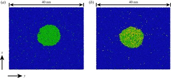
Figure 1. Examples of instantaneous snapshots of simulation results for dissolving droplets. (a) Binary system (or single-component drop) and (b) ternary system (or multicomponent drop). Throughout the paper, the blue particles (which form the bulk liquid) are labelled ‘1’, while green and yellow particles (which form the drop) are labelled 2 and 3, respectively. The nanodrops shown in the figure are sections of a cylinder with the $z$
-axis normal to the page and inwards.
$z$
-axis normal to the page and inwards.
The interaction between the particles is described by a Lennard-Jones potential,
 $$\begin{eqnarray}\displaystyle \unicode[STIX]{x1D719}_{ij}(r)=4\unicode[STIX]{x1D716}_{ij}\left[\left(\frac{\unicode[STIX]{x1D70E}_{ij}}{r}\right)^{12}-\left(\frac{\unicode[STIX]{x1D70E}_{ij}}{r}\right)^{6}\right], & & \displaystyle\end{eqnarray}$$
where $\unicode[STIX]{x1D716}_{ij}$
is the interaction strength between particles of types
$\unicode[STIX]{x1D716}_{ij}$
is the interaction strength between particles of types $i$
and
$i$
and $j$
,
$j$
, $\unicode[STIX]{x1D70E}_{ij}$
is the characteristic size of the particles and
$\unicode[STIX]{x1D70E}_{ij}$
is the characteristic size of the particles and $r$
is the distance between the two molecules. The potential is truncated at a relatively large cutoff radius (
$r$
is the distance between the two molecules. The potential is truncated at a relatively large cutoff radius ( $r_{c}$
) of
$r_{c}$
) of $5\unicode[STIX]{x1D70E}_{11}$
. The time step for updating the particle velocities and positions was set at
$5\unicode[STIX]{x1D70E}_{11}$
. The time step for updating the particle velocities and positions was set at $\unicode[STIX]{x1D6FF}t=\unicode[STIX]{x1D70E}_{11}\sqrt{(m_{1}/\unicode[STIX]{x1D716}_{11})}/400$
, where
$\unicode[STIX]{x1D6FF}t=\unicode[STIX]{x1D70E}_{11}\sqrt{(m_{1}/\unicode[STIX]{x1D716}_{11})}/400$
, where $m_{1}$
is the mass of the bulk liquid particles and
$m_{1}$
is the mass of the bulk liquid particles and $\unicode[STIX]{x1D716}_{11}$
is their mutual Lennard-Jones interaction parameter. The time step was chosen so that its value is sufficiently smaller than the shortest time scale available in the system (Frenkel & Smit Reference Frenkel and Smit2002). Periodic boundary conditions were employed in all three directions, with the box length in the
$\unicode[STIX]{x1D716}_{11}$
is their mutual Lennard-Jones interaction parameter. The time step was chosen so that its value is sufficiently smaller than the shortest time scale available in the system (Frenkel & Smit Reference Frenkel and Smit2002). Periodic boundary conditions were employed in all three directions, with the box length in the $z$
direction (
$z$
direction ( ${\sim}15\unicode[STIX]{x1D70E}$
, typically 5.6 nm) so much shorter than in the other two directions (
${\sim}15\unicode[STIX]{x1D70E}$
, typically 5.6 nm) so much shorter than in the other two directions ( ${\sim}120\unicode[STIX]{x1D70E}$
, typically 40 nm) that the drop approximates a short section of a cylinder.
${\sim}120\unicode[STIX]{x1D70E}$
, typically 40 nm) that the drop approximates a short section of a cylinder.
The simulations were performed in an $NPT$
ensemble where the temperature was fixed at
$NPT$
ensemble where the temperature was fixed at $300K$
, which is below the critical point for the Lennard-Jones parameters (
$300K$
, which is below the critical point for the Lennard-Jones parameters ( $\unicode[STIX]{x1D70E}_{ij}$
,
$\unicode[STIX]{x1D70E}_{ij}$
, $\unicode[STIX]{x1D716}_{ij}$
) that we have chosen. Semi-isotropic pressure coupling was used for maintaining constant pressure: the simulation box expands or contracts only in the
$\unicode[STIX]{x1D716}_{ij}$
) that we have chosen. Semi-isotropic pressure coupling was used for maintaining constant pressure: the simulation box expands or contracts only in the $x$
- and
$x$
- and $y$
-directions to keep the pressure constant. This was done to prevent the change in the system configuration from quasi-two-dimensional to three-dimensional. The complete set of Lennard-Jones parameters that we used in our simulations is given in table 1. The total number of particles in a typical simulation box is approximately 110 000, out of which approximately 12 000 form the drop phase at initial time. The velocities of particles are initialised from the Maxwell–Boltzmann distribution for a temperature of 300 K.
$y$
-directions to keep the pressure constant. This was done to prevent the change in the system configuration from quasi-two-dimensional to three-dimensional. The complete set of Lennard-Jones parameters that we used in our simulations is given in table 1. The total number of particles in a typical simulation box is approximately 110 000, out of which approximately 12 000 form the drop phase at initial time. The velocities of particles are initialised from the Maxwell–Boltzmann distribution for a temperature of 300 K.
Table 1. Value of various Lennard-Jones parameters used in the MD simulations. The interaction parameter $\unicode[STIX]{x1D716}_{23}$
between type-2 and type-3 particles was varied between 3.6 to
$\unicode[STIX]{x1D716}_{23}$
between type-2 and type-3 particles was varied between 3.6 to $4.1~\text{kJ}~\text{mol}^{-1}$
for the multicomponent drop simulations.
$4.1~\text{kJ}~\text{mol}^{-1}$
for the multicomponent drop simulations.
The time-dependent average density field of the type-2 and type-3 particles was calculated, correcting for the centre of mass motion in the lateral direction, and then averaged to give an average local density $\unicode[STIX]{x1D70C}(r)$
. The radius of curvature of the drop was then obtained by fitting a circle to the 0.5 iso-density contour of the normalised density
$\unicode[STIX]{x1D70C}(r)$
. The radius of curvature of the drop was then obtained by fitting a circle to the 0.5 iso-density contour of the normalised density $(\unicode[STIX]{x1D70C}(r)-\unicode[STIX]{x1D70C}_{B})/(\unicode[STIX]{x1D70C}_{D}-\unicode[STIX]{x1D70C}_{B})$
, with
$(\unicode[STIX]{x1D70C}(r)-\unicode[STIX]{x1D70C}_{B})/(\unicode[STIX]{x1D70C}_{D}-\unicode[STIX]{x1D70C}_{B})$
, with $\unicode[STIX]{x1D70C}_{D}$
and
$\unicode[STIX]{x1D70C}_{D}$
and $\unicode[STIX]{x1D70C}_{B}$
the mean densities of the drop and bulk liquid. The use of iso-density contours around 0.5 would have a negligible effect on the results.
$\unicode[STIX]{x1D70C}_{B}$
the mean densities of the drop and bulk liquid. The use of iso-density contours around 0.5 would have a negligible effect on the results.
3 Macroscopic modelling
In this section, we model the dissolution of a single-component and a multicomponent drop in a host liquid using the macroscopic time-dependent diffusion equation to gain insights useful for interpretation of MD simulations. Since the solubility of the bulk liquid in the drop constituents is very small, we assume that it is perfectly immiscible with the drop constituents. We first address the case of a single-component drop for which the interface concentration is constant and equal to the solubility of that component in the bulk liquid, and later discuss the case of a multicomponent drop for which the concentration at the interface changes with time.
3.1 Single-component drop
In the single-component case the drop and the surrounding bulk liquid consist of particles of type 2 and 1, respectively. At time $t=0$
, the bulk liquid has some initial concentration
$t=0$
, the bulk liquid has some initial concentration $c_{0}$
of type-2 particles:
$c_{0}$
of type-2 particles:
 $$\begin{eqnarray}\displaystyle c(r,0)=c_{0}. & & \displaystyle\end{eqnarray}$$
At subsequent times, the concentration $c$
of type-2 particles in the bulk liquid evolves according to the diffusion equation
$c$
of type-2 particles in the bulk liquid evolves according to the diffusion equation
 $$\begin{eqnarray}\displaystyle \frac{\unicode[STIX]{x2202}c}{\unicode[STIX]{x2202}t}=\frac{D_{21}}{r}\frac{\unicode[STIX]{x2202}}{\unicode[STIX]{x2202}r}\left(r\frac{\unicode[STIX]{x2202}c}{\unicode[STIX]{x2202}r}\right), & & \displaystyle\end{eqnarray}$$
where $D_{21}$
is the diffusivity of type-2 particles in the bulk liquid, and
$D_{21}$
is the diffusivity of type-2 particles in the bulk liquid, and $r$
is the radial coordinate measured from the axis of the drop. At the surface of the drop,
$r$
is the radial coordinate measured from the axis of the drop. At the surface of the drop, $r=R$
, the concentration remains constant and equal to the solubility of the type-2 particles in the bulk liquid:
$r=R$
, the concentration remains constant and equal to the solubility of the type-2 particles in the bulk liquid:
 $$\begin{eqnarray}\displaystyle c(R,t)=c_{s}. & & \displaystyle\end{eqnarray}$$
In the MD simulations, the drop is in a rectangular box and periodic boundary conditions are used, i.e. any particle ‘leaving’ the system at a boundary will enter it at the opposite boundary so that the total number of particles in the system is conserved. To mimic this set-up in the macroscopic diffusion setting, we solve the diffusion equation (3.2) in a finite cylindrical domain of radius $R_{b}$
enforcing the conservation of the total amount of solute by imposing that the flux of type-2 particles at
$R_{b}$
enforcing the conservation of the total amount of solute by imposing that the flux of type-2 particles at $r=R_{b}$
vanishes:
$r=R_{b}$
vanishes:
 $$\begin{eqnarray}\displaystyle \left.\frac{\unicode[STIX]{x2202}c(r,t)}{\unicode[STIX]{x2202}r}\right|_{r=R_{b}}=0. & & \displaystyle\end{eqnarray}$$ $R_{b}$
is chosen so that
$R_{b}$
is chosen so that $\unicode[STIX]{x03C0}R_{b}^{2}$
equals the area of the cross-section of the MD computational domain.
$\unicode[STIX]{x03C0}R_{b}^{2}$
equals the area of the cross-section of the MD computational domain.
The mathematical problem described can be solved analytically by means of the Laplace transform; the detailed solution is described in Carslaw & Jaeger (Reference Carslaw and Jaeger1959) and Prosperetti (Reference Prosperetti2011). The concentration profile $c(r,t)$
as a function of radial distance and time is given by
$c(r,t)$
as a function of radial distance and time is given by
 $$\begin{eqnarray}\displaystyle \frac{c(r,t)-c_{0}}{c_{s}-c_{0}}=1-\unicode[STIX]{x03C0}\mathop{\sum }_{n=1}^{\infty }\text{e}^{-D_{21}\unicode[STIX]{x1D6FC}_{n}^{2}t}G(R,\unicode[STIX]{x1D6FC}_{n})(\text{J}_{0}(r\unicode[STIX]{x1D6FC}_{n})\text{Y}_{0}(R\unicode[STIX]{x1D6FC}_{n})-\text{Y}_{0}(r\unicode[STIX]{x1D6FC}_{n})\text{J}_{0}(R\unicode[STIX]{x1D6FC}_{n})), & & \displaystyle\end{eqnarray}$$
where
 $$\begin{eqnarray}\displaystyle G(R,\unicode[STIX]{x1D6FC}_{n})=\frac{\text{J}_{1}^{2}(R_{b}\unicode[STIX]{x1D6FC}_{n})}{\text{J}_{1}^{2}(R_{b}\unicode[STIX]{x1D6FC}_{n})-\text{J}_{0}^{2}(R\unicode[STIX]{x1D6FC}_{n})} & & \displaystyle\end{eqnarray}$$
and $\text{J}_{0,1}$
and
$\text{J}_{0,1}$
and $\text{Y}_{0}$
are Bessel functions of the first kind and second kind, respectively and
$\text{Y}_{0}$
are Bessel functions of the first kind and second kind, respectively and $\{\unicode[STIX]{x1D6FC}_{1},\unicode[STIX]{x1D6FC}_{2}\ldots \}$
are the solutions of
$\{\unicode[STIX]{x1D6FC}_{1},\unicode[STIX]{x1D6FC}_{2}\ldots \}$
are the solutions of
 $$\begin{eqnarray}\displaystyle \text{J}_{0}(R\unicode[STIX]{x1D6FC})\text{Y}_{1}(R_{b}\unicode[STIX]{x1D6FC})-\text{Y}_{0}(R\unicode[STIX]{x1D6FC})\text{J}_{1}(R_{b}\unicode[STIX]{x1D6FC})=0. & & \displaystyle\end{eqnarray}$$
The dissolution rate, or the rate of change of the drop mass $M=\unicode[STIX]{x03C0}R^{2}\unicode[STIX]{x1D70C}_{D}$
, is determined by calculating the flux at the interface boundary:
$M=\unicode[STIX]{x03C0}R^{2}\unicode[STIX]{x1D70C}_{D}$
, is determined by calculating the flux at the interface boundary:
 $$\begin{eqnarray}\displaystyle \frac{\text{d}M}{\text{d}t}=-2\unicode[STIX]{x03C0}R\left(-D_{21}\left.\frac{\unicode[STIX]{x2202}c(r,t)}{\unicode[STIX]{x2202}r}\right|_{r=R}\right). & & \displaystyle\end{eqnarray}$$
By substituting (3.5) in (3.8), equation (3.8) gives that the rate of change of the drop radius is given by
 $$\begin{eqnarray}\displaystyle \frac{\text{d}R}{\text{d}t}=\frac{2D_{21}(c_{s}-c_{0})}{\unicode[STIX]{x1D70C}_{D}R}\mathop{\sum }_{n=1}^{\infty }\text{e}^{-D_{21}\unicode[STIX]{x1D6FC}_{n}^{2}t}G(R,\unicode[STIX]{x1D6FC}_{n}). & & \displaystyle\end{eqnarray}$$
Note that (3.8) comes from the solution of the diffusion equation with fixed drop radius while the drop radius itself is changing with time during dissolution. However, due to the slow diffusive dissolution process and resulting separation of time scales, it is a reasonable approximation to use the solution of the fixed boundary problem for the drop (Epstein & Plesset Reference Epstein and Plesset1950).
3.2 Multicomponent drop
The diffusion time $t_{diff}$
of the drop constituents over the drop radius is of the order of
$t_{diff}$
of the drop constituents over the drop radius is of the order of $t_{diff}\sim R^{2}/D_{23}$
, while the time scale
$t_{diff}\sim R^{2}/D_{23}$
, while the time scale $t_{diss}$
for the drop dissolution can be estimated as
$t_{diss}$
for the drop dissolution can be estimated as $t_{diss}\sim (\unicode[STIX]{x03C0}R^{2}\unicode[STIX]{x1D70C}_{D})/(2\unicode[STIX]{x03C0}RD_{21}(c_{s}-c_{0}))=(R^{2}/2D_{21})[\unicode[STIX]{x1D70C}_{D}/(c_{s}-c_{0})]$
. The ratio of these two time scales is therefore
$t_{diss}\sim (\unicode[STIX]{x03C0}R^{2}\unicode[STIX]{x1D70C}_{D})/(2\unicode[STIX]{x03C0}RD_{21}(c_{s}-c_{0}))=(R^{2}/2D_{21})[\unicode[STIX]{x1D70C}_{D}/(c_{s}-c_{0})]$
. The ratio of these two time scales is therefore $t_{diff}/t_{diss}\sim (2D_{21}/D_{23})[(c_{s}-c_{0})/\unicode[STIX]{x1D70C}_{D}]$
, which is very small. This remark justifies the assumption that the drop composition remains spatially uniform which we adopt. Note that we did not use the diffusion equation within the drop because of the large difference in the two time scales as explained. Also the Fickian diffusion framework provided above is valid only for dilute concentrations of the components in the bulk liquid, while in the drop phase the concentration of both components is quite high. The applicability of the diffusion equation for such a non-ideal system is studied in detail by Philippi et al. (Reference Philippi, Mattila, Siebert, dos Santos, Júnior and Surmas2012), but it is not relevant for the scientific question addressed here. For a two-component drop, we should solve (3.2) for each component subject to the same boundary conditions at
$t_{diff}/t_{diss}\sim (2D_{21}/D_{23})[(c_{s}-c_{0})/\unicode[STIX]{x1D70C}_{D}]$
, which is very small. This remark justifies the assumption that the drop composition remains spatially uniform which we adopt. Note that we did not use the diffusion equation within the drop because of the large difference in the two time scales as explained. Also the Fickian diffusion framework provided above is valid only for dilute concentrations of the components in the bulk liquid, while in the drop phase the concentration of both components is quite high. The applicability of the diffusion equation for such a non-ideal system is studied in detail by Philippi et al. (Reference Philippi, Mattila, Siebert, dos Santos, Júnior and Surmas2012), but it is not relevant for the scientific question addressed here. For a two-component drop, we should solve (3.2) for each component subject to the same boundary conditions at $r=R_{b}$
and similar initial conditions. A difference with respect to the single-component case arises because the concentration of each component at the interface depends on the drop composition, which changes with time. To deal with this feature we use Duhamel’s principle (Carslaw & Jaeger Reference Carslaw and Jaeger1959; Prosperetti Reference Prosperetti2011) to convert the solution of the diffusion equation obtained with a time-independent boundary condition to the case when the boundary condition is a function of time. We write the time-dependent boundary condition for the concentration as
$r=R_{b}$
and similar initial conditions. A difference with respect to the single-component case arises because the concentration of each component at the interface depends on the drop composition, which changes with time. To deal with this feature we use Duhamel’s principle (Carslaw & Jaeger Reference Carslaw and Jaeger1959; Prosperetti Reference Prosperetti2011) to convert the solution of the diffusion equation obtained with a time-independent boundary condition to the case when the boundary condition is a function of time. We write the time-dependent boundary condition for the concentration as
 $$\begin{eqnarray}\displaystyle c_{i}(R,t)=c_{s,i}\unicode[STIX]{x1D719}_{i}(t), & & \displaystyle\end{eqnarray}$$
where $i=2,3$
refers to the two components of the drop and
$i=2,3$
refers to the two components of the drop and $\unicode[STIX]{x1D719}_{i}(t)$
is a normalised function describing the variation of the interface concentration with time. Then, according to Duhamel’s principle, the concentration profile of each component in the bulk liquid is given by
$\unicode[STIX]{x1D719}_{i}(t)$
is a normalised function describing the variation of the interface concentration with time. Then, according to Duhamel’s principle, the concentration profile of each component in the bulk liquid is given by
 $$\begin{eqnarray}\displaystyle c_{i}(r,t)=\int _{0}^{t}\unicode[STIX]{x1D719}_{i}(\unicode[STIX]{x1D706})\frac{\unicode[STIX]{x2202}}{\unicode[STIX]{x2202}t}c_{const.,i}(r,t-\unicode[STIX]{x1D706})\,\text{d}\unicode[STIX]{x1D706}, & & \displaystyle\end{eqnarray}$$
where $c_{const,i}(r,t)$
is the solution of the diffusion equation for a fixed boundary condition
$c_{const,i}(r,t)$
is the solution of the diffusion equation for a fixed boundary condition $c_{const,i}(R,t)=c_{s,i}$
, which is given by (3.5) with
$c_{const,i}(R,t)=c_{s,i}$
, which is given by (3.5) with $c_{s}$
replaced by
$c_{s}$
replaced by $c_{s,i}$
. The rate of change of mass of each component follows then from the flux at the liquid–liquid interface similarly to (3.8),
$c_{s,i}$
. The rate of change of mass of each component follows then from the flux at the liquid–liquid interface similarly to (3.8),
 $$\begin{eqnarray}\displaystyle \frac{\text{d}M_{i}}{\text{d}t}=-2\unicode[STIX]{x03C0}R\left(-D_{i1}\left.\frac{\unicode[STIX]{x2202}c_{i}(r,t)}{\unicode[STIX]{x2202}r}\right|_{r=R}\right). & & \displaystyle\end{eqnarray}$$
The concentration of each component in the bulk liquid is calculated by substituting (3.5) in (3.11), which is further substituted in (3.12) to obtain the rate of change of the mass of each constituent of the drop,
 $$\begin{eqnarray}\displaystyle \frac{\text{d}M_{i}}{\text{d}t}=4\unicode[STIX]{x03C0}D_{i1}\mathop{\sum }_{n=1}^{\infty }\text{e}^{-D_{i1}\unicode[STIX]{x1D6FC}_{n}^{2}t}G(R,\unicode[STIX]{x1D6FC}_{n})\left(c_{s,i}\unicode[STIX]{x1D719}_{i}(0)-c_{0,i}+\int _{0}^{t}c_{s,i}\unicode[STIX]{x1D719}_{i}^{\prime }(\unicode[STIX]{x1D706})\text{e}^{D_{i1}\unicode[STIX]{x1D6FC}_{n}^{2}\unicode[STIX]{x1D706}}\,\text{d}\unicode[STIX]{x1D706}\right). & & \displaystyle\end{eqnarray}$$
The rate of change of the radius of the multicomponent drop can then be calculated from the rate of change of mass of each component via
 $$\begin{eqnarray}\displaystyle 2\unicode[STIX]{x03C0}R\frac{\text{d}R}{\text{d}t}=\frac{1}{\unicode[STIX]{x1D70C}_{0,2}}\frac{\text{d}M_{2}}{\text{d}t}+\frac{1}{\unicode[STIX]{x1D70C}_{0,3}}\frac{\text{d}M_{3}}{\text{d}t}, & & \displaystyle\end{eqnarray}$$
where $\unicode[STIX]{x1D70C}_{0,2}$
and
$\unicode[STIX]{x1D70C}_{0,2}$
and $\unicode[STIX]{x1D70C}_{0,3}$
are the densities of the pure components 2 and 3, respectively. Here we neglect the volume change due to the mixing of two components.
$\unicode[STIX]{x1D70C}_{0,3}$
are the densities of the pure components 2 and 3, respectively. Here we neglect the volume change due to the mixing of two components.
3.3 Macroscopic model parameters
3.3.1 Interface concentration
As shown in § 3.2, the concentration of both components at the liquid–liquid interface is required as a boundary condition to solve the diffusion equation. The solubility $c_{s}$
of component 2 in a bulk liquid of component 1 is calculated from independent MD simulations, from which we obtain the values
$c_{s}$
of component 2 in a bulk liquid of component 1 is calculated from independent MD simulations, from which we obtain the values $13.612~\text{kg}~\text{m}^{-3}$
and
$13.612~\text{kg}~\text{m}^{-3}$
and $62.416~\text{kg}~\text{m}^{-3}$
for interaction strengths
$62.416~\text{kg}~\text{m}^{-3}$
for interaction strengths $\unicode[STIX]{x1D716}_{12}=2.5$
and
$\unicode[STIX]{x1D716}_{12}=2.5$
and $\unicode[STIX]{x1D716}_{12}=2.8$
, respectively. However, for a multicomponent drop,
$\unicode[STIX]{x1D716}_{12}=2.8$
, respectively. However, for a multicomponent drop, $c_{s,i}$
is a function of the composition of the drop, which changes substantially during the dissolution. In principle, this function can be calculated from the local thermodynamic equilibrium condition, which requires equating the chemical potential of each component on the two sides of the interface. Expressions for the chemical potentials of ternary system of Lennard-Jones particles which we are using are not available. Thus, we chose to perform independent ‘numerical experiments’ in order to get the interface concentration of each component as a function of the drop composition. The procedure is to set up a multicomponent drop in a bulk liquid and to allow the system to reach equilibrium. In this situation, equilibrium is achieved when the concentrations of both components in the bulk liquid reach steady state and the drop does not dissolve further. Steady state ensures that the concentrations of both components in the bulk liquid attain their solubility value. At this point the solubilities of the drop components and the drop composition can be determined. In order to reduce statistical errors, and to cover the entire range of mole fractions
$c_{s,i}$
is a function of the composition of the drop, which changes substantially during the dissolution. In principle, this function can be calculated from the local thermodynamic equilibrium condition, which requires equating the chemical potential of each component on the two sides of the interface. Expressions for the chemical potentials of ternary system of Lennard-Jones particles which we are using are not available. Thus, we chose to perform independent ‘numerical experiments’ in order to get the interface concentration of each component as a function of the drop composition. The procedure is to set up a multicomponent drop in a bulk liquid and to allow the system to reach equilibrium. In this situation, equilibrium is achieved when the concentrations of both components in the bulk liquid reach steady state and the drop does not dissolve further. Steady state ensures that the concentrations of both components in the bulk liquid attain their solubility value. At this point the solubilities of the drop components and the drop composition can be determined. In order to reduce statistical errors, and to cover the entire range of mole fractions $0\leqslant x_{2,3}\leqslant 1$
, it is necessary to carry out many such simulations (on the order of 100). Since our interest is in studying the effect of different interaction parameters
$0\leqslant x_{2,3}\leqslant 1$
, it is necessary to carry out many such simulations (on the order of 100). Since our interest is in studying the effect of different interaction parameters $\unicode[STIX]{x1D716}_{23}$
, these simulation must be repeated for each value of this parameter. The computational burden of this procedure is therefore quite substantial and, in order to reduce it, it was necessary to use systems much smaller than those of actual interest (
$\unicode[STIX]{x1D716}_{23}$
, these simulation must be repeated for each value of this parameter. The computational burden of this procedure is therefore quite substantial and, in order to reduce it, it was necessary to use systems much smaller than those of actual interest ( ${\sim}$
10 % of the total number of particles used in the drop dissolution simulations). While this choice renders the calculation feasible, it has a significant downside, as will be explained later. Typical examples of the results are given in figure 2, which shows the component solubility curves for
${\sim}$
10 % of the total number of particles used in the drop dissolution simulations). While this choice renders the calculation feasible, it has a significant downside, as will be explained later. Typical examples of the results are given in figure 2, which shows the component solubility curves for $\unicode[STIX]{x1D716}_{23}=3.6~\text{kJ}~\text{mol}^{-1}$
and
$\unicode[STIX]{x1D716}_{23}=3.6~\text{kJ}~\text{mol}^{-1}$
and $\unicode[STIX]{x1D716}_{23}=4.1~\text{kJ}~\text{mol}^{-1}$
. It can be seen that the statistical fluctuations introduce significant uncertainties. The black lines show the result of a least-squares fit of a cubic polynomial to the numerical result: this fit will be used in the macroscopic model.
$\unicode[STIX]{x1D716}_{23}=4.1~\text{kJ}~\text{mol}^{-1}$
. It can be seen that the statistical fluctuations introduce significant uncertainties. The black lines show the result of a least-squares fit of a cubic polynomial to the numerical result: this fit will be used in the macroscopic model.
Figure 2. Normalised solubilities of the drop constituents in the bulk liquid as functions of the drop composition; (a) is for strongly interacting constituents, $\unicode[STIX]{x1D716}_{23}=4.1~\text{kJ}~\text{mol}^{-1}$
, while (b) is for weakly interacting particles,
$\unicode[STIX]{x1D716}_{23}=4.1~\text{kJ}~\text{mol}^{-1}$
, while (b) is for weakly interacting particles, $\unicode[STIX]{x1D716}_{23}=3.6~\text{kJ}~\text{mol}^{-1}$
. The red points are the MD data averaged over many simulations; the error bars give the standard deviations of several realisations. The black curves show a least-squares cubic polynomial fit to the MD simulation results. These fits have been used to set the boundary condition at the drop surface in the macroscopic diffusion model.
$\unicode[STIX]{x1D716}_{23}=3.6~\text{kJ}~\text{mol}^{-1}$
. The red points are the MD data averaged over many simulations; the error bars give the standard deviations of several realisations. The black curves show a least-squares cubic polynomial fit to the MD simulation results. These fits have been used to set the boundary condition at the drop surface in the macroscopic diffusion model.
3.3.2 Diffusion constants
As can be observed from the (3.9) and (3.13), the values of the diffusion constants $D_{i1}$
of the drop constituents in the bulk liquid are also required to predict the dissolution dynamics. To this end, independent MD simulations were performed for both binary and ternary systems at different concentrations of drop constituents. The diffusion constant of each component was calculated from the mean square displacement of the particles of that component in the bulk liquid (Frenkel & Smit Reference Frenkel and Smit2002). In the case of a single-component drop, the diffusivity
$D_{i1}$
of the drop constituents in the bulk liquid are also required to predict the dissolution dynamics. To this end, independent MD simulations were performed for both binary and ternary systems at different concentrations of drop constituents. The diffusion constant of each component was calculated from the mean square displacement of the particles of that component in the bulk liquid (Frenkel & Smit Reference Frenkel and Smit2002). In the case of a single-component drop, the diffusivity $D_{21}$
is obtained as
$D_{21}$
is obtained as $9.982\times 10^{-9}~\text{m}^{2}~\text{s}^{-1}$
and
$9.982\times 10^{-9}~\text{m}^{2}~\text{s}^{-1}$
and $9.719\times 10^{-9}~\text{m}^{2}~\text{s}^{-1}$
for
$9.719\times 10^{-9}~\text{m}^{2}~\text{s}^{-1}$
for $\unicode[STIX]{x1D716}_{12}=2.5$
and
$\unicode[STIX]{x1D716}_{12}=2.5$
and $\unicode[STIX]{x1D716}_{12}=2.8$
, respectively. For a multicomponent drop, the diffusivity of components 2 and 3 in the bulk liquid is obtained as
$\unicode[STIX]{x1D716}_{12}=2.8$
, respectively. For a multicomponent drop, the diffusivity of components 2 and 3 in the bulk liquid is obtained as $D_{21}=9.31\times 10^{-9}~\text{m}^{2}~\text{s}^{-1}$
and
$D_{21}=9.31\times 10^{-9}~\text{m}^{2}~\text{s}^{-1}$
and $D_{31}=10.42\times 10^{-9}~\text{m}^{2}~\text{s}^{-1}$
, respectively, for
$D_{31}=10.42\times 10^{-9}~\text{m}^{2}~\text{s}^{-1}$
, respectively, for $\unicode[STIX]{x1D716}_{23}=3.6$
, and
$\unicode[STIX]{x1D716}_{23}=3.6$
, and $D_{21}=9.34\times 10^{-9}~\text{m}^{2}~\text{s}^{-1}$
and
$D_{21}=9.34\times 10^{-9}~\text{m}^{2}~\text{s}^{-1}$
and $D_{31}=9.84\times 10^{-9}~\text{m}^{2}~\text{s}^{-1}$
, respectively, for
$D_{31}=9.84\times 10^{-9}~\text{m}^{2}~\text{s}^{-1}$
, respectively, for $\unicode[STIX]{x1D716}_{23}=4.1$
. For the sake of comparison, we also give the diffusivity of methanol in water, namely
$\unicode[STIX]{x1D716}_{23}=4.1$
. For the sake of comparison, we also give the diffusivity of methanol in water, namely $D\sim 1.54\times 10^{-9}~\text{m}^{2}~\text{s}^{-1}$
(Hao & Leaist Reference Hao and Leaist1996), which is slightly lower than the diffusivity of the Lennard-Jones particles that we are using. The advantage of a slightly higher diffusivity in our MD simulation is faster convergence, without changing the physics of the process. We did not use the Maxwell–Stefan theory for multicomponent diffusion for liquid mixtures, as the concentrations of type-2 and type-3 particles in the bulk liquid are so low that the flux of one component has a negligible effect on the other (van de Ven-Lucassen et al.
Reference van de Ven-Lucassen, Vlugt, van der Zanden and Kerkhof1998). Note also that we assumed the values of the diffusivities are independent of the concentration. It is a reasonable assumption, as the concentration of both components in the bulk liquid is quite low and has negligible effect on the values of the diffusivities (Hao & Leaist Reference Hao and Leaist1996).
$D\sim 1.54\times 10^{-9}~\text{m}^{2}~\text{s}^{-1}$
(Hao & Leaist Reference Hao and Leaist1996), which is slightly lower than the diffusivity of the Lennard-Jones particles that we are using. The advantage of a slightly higher diffusivity in our MD simulation is faster convergence, without changing the physics of the process. We did not use the Maxwell–Stefan theory for multicomponent diffusion for liquid mixtures, as the concentrations of type-2 and type-3 particles in the bulk liquid are so low that the flux of one component has a negligible effect on the other (van de Ven-Lucassen et al.
Reference van de Ven-Lucassen, Vlugt, van der Zanden and Kerkhof1998). Note also that we assumed the values of the diffusivities are independent of the concentration. It is a reasonable assumption, as the concentration of both components in the bulk liquid is quite low and has negligible effect on the values of the diffusivities (Hao & Leaist Reference Hao and Leaist1996).
Figure 3. Radius versus time for a dissolving drop in a binary system for two different interaction strengths between the components. Red and green points are data obtained from the MD simulations while the black curves represent the dissolution curve within the macroscopic diffusion model.
4 Results and discussion
In this section we compare the radius of the drop obtained from MD simulations with the theoretical predictions derived in §§ 3.1 and 3.2. The role of the interaction strength between the two components of a multicomponent drop and the effect of the drop curvature on the dissolution dynamics are discussed.
4.1 Single-component drop
We first simulated a binary system in which component 1 forms the bulk liquid and component 2 forms the drop. Initially, the concentration of component 2 in the bulk liquid is set below its solubility while, at the liquid–liquid interface, the concentration of the component 2 is equal to its solubility. We performed the simulation for two different solubilities, as shown in figure 3. The solubility of the component is changed by changing the interaction parameter $\unicode[STIX]{x1D716}_{12}$
in the Lennard-Jones potential; component 2 can be made more soluble by increasing the value of this parameter. The drop consisting of the more soluble component dissolves faster as expected, and evident from figure 3. The solid lines in figure 3 show the radius of the drop as predicted from the macroscopic diffusion equation (3.9), via the solution procedure outlined in § 3.1. We find excellent agreement between the MD simulation data and the theoretical result.
$\unicode[STIX]{x1D716}_{12}$
in the Lennard-Jones potential; component 2 can be made more soluble by increasing the value of this parameter. The drop consisting of the more soluble component dissolves faster as expected, and evident from figure 3. The solid lines in figure 3 show the radius of the drop as predicted from the macroscopic diffusion equation (3.9), via the solution procedure outlined in § 3.1. We find excellent agreement between the MD simulation data and the theoretical result.
4.2 Multicomponent drop
For the multicomponent case, initially the drop consists of equal parts of components 2 and 3 and their concentration in the bulk liquid is below the equilibrium concentration corresponding to the initial mole fraction. The two drop components have very different solubilities in the bulk liquid as a consequence of a different interaction parameter, $\unicode[STIX]{x1D716}_{21}$
and
$\unicode[STIX]{x1D716}_{21}$
and $\unicode[STIX]{x1D716}_{31}$
, provided in table 1, while the interaction between the two components of the drop (
$\unicode[STIX]{x1D716}_{31}$
, provided in table 1, while the interaction between the two components of the drop ( $\unicode[STIX]{x1D716}_{23}$
) adds another dimension to the dissolution dynamics. We performed MD simulations for different values of
$\unicode[STIX]{x1D716}_{23}$
) adds another dimension to the dissolution dynamics. We performed MD simulations for different values of $\unicode[STIX]{x1D716}_{23}$
while keeping all other interaction parameters the same (see table 1). Several examples of the radius-versus-time of the drop for different values of
$\unicode[STIX]{x1D716}_{23}$
while keeping all other interaction parameters the same (see table 1). Several examples of the radius-versus-time of the drop for different values of $\unicode[STIX]{x1D716}_{23}$
are shown in figure 4. It can be observed that increasing
$\unicode[STIX]{x1D716}_{23}$
are shown in figure 4. It can be observed that increasing $\unicode[STIX]{x1D716}_{23}$
leads to a slower dissolution rate. This behaviour is expected, as a higher interaction strength between the two drop constituents tends to hinder the particles leaving the drop phase. Recently, Dietrich et al. (Reference Dietrich, Rump, Lv, Kooij, Zandvliet and Lohse2017) also showed similar experimental results in which the interaction between the two components of the sessile drop leads to a decrease of the dissolution rate compared to the dissolution of a pure component. Since the amount of bulk liquid is limited, the drops do not dissolve completely, and the radius stabilises when equilibrium is achieved.
$\unicode[STIX]{x1D716}_{23}$
leads to a slower dissolution rate. This behaviour is expected, as a higher interaction strength between the two drop constituents tends to hinder the particles leaving the drop phase. Recently, Dietrich et al. (Reference Dietrich, Rump, Lv, Kooij, Zandvliet and Lohse2017) also showed similar experimental results in which the interaction between the two components of the sessile drop leads to a decrease of the dissolution rate compared to the dissolution of a pure component. Since the amount of bulk liquid is limited, the drops do not dissolve completely, and the radius stabilises when equilibrium is achieved.
Figure 4. Radius of a dissolving multicomponent drop as a function of time for various interaction strengths $\unicode[STIX]{x1D716}_{23}$
between the drop constituents resulting from the MD simulations.
$\unicode[STIX]{x1D716}_{23}$
between the drop constituents resulting from the MD simulations.
We can now attempt to reproduce the dissolution dynamics of a multicomponent drop with the macroscopic model as we did before in the single-component case. Note that (3.14) requires the interface concentration of each component as a function of time, which is implicitly known as a function of the mole fraction for which we use the polynomial fit as explained before. The results for the time dependence of the drop radius, shown by the black lines in figure 5, are compared with the results of the MD simulations for two interaction strengths $\unicode[STIX]{x1D716}_{23}$
. The results of the macroscopic theory closely mimic the MD results for the stronger interaction between the drop constituents,
$\unicode[STIX]{x1D716}_{23}$
. The results of the macroscopic theory closely mimic the MD results for the stronger interaction between the drop constituents, $\unicode[STIX]{x1D716}_{23}=4.1~\text{kJ}~\text{mol}^{-1}$
, but visible differences are observed for the weaker interaction strength,
$\unicode[STIX]{x1D716}_{23}=4.1~\text{kJ}~\text{mol}^{-1}$
, but visible differences are observed for the weaker interaction strength, $\unicode[STIX]{x1D716}_{23}=3.6~\text{kJ}~\text{mol}^{-1}$
.
$\unicode[STIX]{x1D716}_{23}=3.6~\text{kJ}~\text{mol}^{-1}$
.
Figure 5. Radius versus time for a dissolving drop in a ternary system for two different interaction strengths between the drop constituents. The red and green points are obtained from the MD simulations with $\unicode[STIX]{x1D716}_{23}=4.1~\text{kJ}~\text{mol}^{-1}$
and
$\unicode[STIX]{x1D716}_{23}=4.1~\text{kJ}~\text{mol}^{-1}$
and $\unicode[STIX]{x1D716}_{23}=3.6~\text{kJ}~\text{mol}^{-1}$
, respectively. The black curves represent the results of the macroscopic diffusion model.
$\unicode[STIX]{x1D716}_{23}=3.6~\text{kJ}~\text{mol}^{-1}$
, respectively. The black curves represent the results of the macroscopic diffusion model.
In an effort to understand the origin of the difference we were led to study the spatial distribution of the drop constituents inside the drop. Typical results are shown in figure 6 for different values of $\unicode[STIX]{x1D716}_{23}$
and
$\unicode[STIX]{x1D716}_{23}$
and $\unicode[STIX]{x1D716}_{21}=2.5~\text{kJ}~\text{mol}^{-1}$
,
$\unicode[STIX]{x1D716}_{21}=2.5~\text{kJ}~\text{mol}^{-1}$
, $\unicode[STIX]{x1D716}_{31}=2.8~\text{kJ}~\text{mol}^{-1}$
. As
$\unicode[STIX]{x1D716}_{31}=2.8~\text{kJ}~\text{mol}^{-1}$
. As $\unicode[STIX]{x1D716}_{23}$
varies, the dissolution dynamics also varies as shown in figure 4. Therefore, in order to generate these graphs the concentration of the components 2 and 3 corresponding to different cases were shifted to superimpose the positions of the drop surface. The graphs in this figure focus on the concentration distribution over a length of
$\unicode[STIX]{x1D716}_{23}$
varies, the dissolution dynamics also varies as shown in figure 4. Therefore, in order to generate these graphs the concentration of the components 2 and 3 corresponding to different cases were shifted to superimpose the positions of the drop surface. The graphs in this figure focus on the concentration distribution over a length of $20\unicode[STIX]{x1D70E}$
straddling the interface. In particular, note that
$20\unicode[STIX]{x1D70E}$
straddling the interface. In particular, note that $r/\unicode[STIX]{x1D70E}=0$
corresponds to the position of the interface of the drop. The unexpected finding is that component 2, which is only weakly interacting with the bulk liquid, is distributed fairly uniformly inside the drop, whereas component 3, which interacts more strongly with the bulk liquid, exhibits an increased concentration near the surface for the lower values of
$r/\unicode[STIX]{x1D70E}=0$
corresponds to the position of the interface of the drop. The unexpected finding is that component 2, which is only weakly interacting with the bulk liquid, is distributed fairly uniformly inside the drop, whereas component 3, which interacts more strongly with the bulk liquid, exhibits an increased concentration near the surface for the lower values of $\unicode[STIX]{x1D716}_{23}$
. In other words, as the mutual interaction between the drop constituents decreases, the stronger affinity of component 3 with the bulk liquid causes it to become denser near the interface. By averaging over several time snapshots we have convinced ourselves that this increase in the local concentration is a robust feature rather than the mere result of statistical fluctuations.
$\unicode[STIX]{x1D716}_{23}$
. In other words, as the mutual interaction between the drop constituents decreases, the stronger affinity of component 3 with the bulk liquid causes it to become denser near the interface. By averaging over several time snapshots we have convinced ourselves that this increase in the local concentration is a robust feature rather than the mere result of statistical fluctuations.
This behaviour is the result of two concomitant effects, namely (i) the imbalance between the self-interaction of the drop constituents as determined by $\unicode[STIX]{x1D716}_{22}$
and
$\unicode[STIX]{x1D716}_{22}$
and $\unicode[STIX]{x1D716}_{33}$
vis-á-vis their mutual interaction, i.e.
$\unicode[STIX]{x1D716}_{33}$
vis-á-vis their mutual interaction, i.e. $\unicode[STIX]{x1D716}_{23}$
, and (ii) the stronger affinity between particles of type 3 and 1 with respect to that between particles of type 2 and 1, which, as will be shown, is enhanced by the curvature of the interface.
$\unicode[STIX]{x1D716}_{23}$
, and (ii) the stronger affinity between particles of type 3 and 1 with respect to that between particles of type 2 and 1, which, as will be shown, is enhanced by the curvature of the interface.
It can be understood that a strong increase of the self-interaction parameters $\unicode[STIX]{x1D716}_{22}$
and
$\unicode[STIX]{x1D716}_{22}$
and $\unicode[STIX]{x1D716}_{33}$
with respect to the mutual interaction parameter
$\unicode[STIX]{x1D716}_{33}$
with respect to the mutual interaction parameter $\unicode[STIX]{x1D716}_{23}$
leads to a segregation of the two components. To verify this phenomenon, we performed simulations of a pure mixture consisting only of the two drop components 2 and 3 in a domain with the same size as that used for the dissolution calculation, choosing low values of
$\unicode[STIX]{x1D716}_{23}$
leads to a segregation of the two components. To verify this phenomenon, we performed simulations of a pure mixture consisting only of the two drop components 2 and 3 in a domain with the same size as that used for the dissolution calculation, choosing low values of $\unicode[STIX]{x1D716}_{23}$
. To quantify the degree of segregation, we introduce the coordination number
$\unicode[STIX]{x1D716}_{23}$
. To quantify the degree of segregation, we introduce the coordination number $Z_{ij}$
as the average number of
$Z_{ij}$
as the average number of $j$
-type particles surrounding
$j$
-type particles surrounding $i$
-type particles within a radius of
$i$
-type particles within a radius of $2\unicode[STIX]{x1D70E}$
. Close values of
$2\unicode[STIX]{x1D70E}$
. Close values of $Z_{23}$
and
$Z_{23}$
and $Z_{22}$
indicate that liquids are highly soluble in each other, while a significant difference between
$Z_{22}$
indicate that liquids are highly soluble in each other, while a significant difference between $Z_{23}$
and
$Z_{23}$
and $Z_{22}$
indicates segregation. Some results for
$Z_{22}$
indicates segregation. Some results for $Z_{22}$
and
$Z_{22}$
and $Z_{23}$
versus time are shown in figure 7. For
$Z_{23}$
versus time are shown in figure 7. For $\unicode[STIX]{x1D716}_{23}=3.2~\text{kJ}~\text{mol}^{-1}$
one observes a very rapid and intense segregation. For
$\unicode[STIX]{x1D716}_{23}=3.2~\text{kJ}~\text{mol}^{-1}$
one observes a very rapid and intense segregation. For $\unicode[STIX]{x1D716}_{23}=3.4~\text{kJ}~\text{mol}^{-1}$
the effect is still present, it is equally fast, but its intensity is reduced. For
$\unicode[STIX]{x1D716}_{23}=3.4~\text{kJ}~\text{mol}^{-1}$
the effect is still present, it is equally fast, but its intensity is reduced. For $\unicode[STIX]{x1D716}_{23}=3.6~\text{kJ}~\text{mol}^{-1}$
, which is the smallest value used in the dissolution simulations, we observe only a slight trace of segregation which cannot be expected to have a strong effect on solubility curves of figure 2. In all cases, the time scale for segregation to set in is much shorter than the time scale of interest for drop dissolution.
$\unicode[STIX]{x1D716}_{23}=3.6~\text{kJ}~\text{mol}^{-1}$
, which is the smallest value used in the dissolution simulations, we observe only a slight trace of segregation which cannot be expected to have a strong effect on solubility curves of figure 2. In all cases, the time scale for segregation to set in is much shorter than the time scale of interest for drop dissolution.
Figure 6. Concentration of the drop constituents as a function of the distance from the interface marked by the vertical line. The left and right diagrams are for components 2 and 3, respectively. The colour scale from blue to yellow indicates the mutual interaction between the drop components. $R$
is the radius of the drop.
$R$
is the radius of the drop.
Figure 7. Coordination number $Z_{ij}$
as a function of time for various interaction strengths
$Z_{ij}$
as a function of time for various interaction strengths $\unicode[STIX]{x1D716}_{23}$
between the two drop constituents.
$\unicode[STIX]{x1D716}_{23}$
between the two drop constituents.
The second cause of the increased concentration of the type-3 particles near the interface namely, their stronger affinity with type-1 particles with respect to type-2 particles, is enhanced by the curvature of the interface. To demonstrate this fact we show figure 8, which compares the type-3 particle concentration near the interface for a plane (green) and a circular (red) surface of radius $R=4.5$
nm for
$R=4.5$
nm for $\unicode[STIX]{x1D716}_{23}=3.6~\text{kJ}~\text{mol}^{-1}$
as a function of the distance from the interface marked by the vertical line. As in the previous figure 6, the graph covers only a distance of
$\unicode[STIX]{x1D716}_{23}=3.6~\text{kJ}~\text{mol}^{-1}$
as a function of the distance from the interface marked by the vertical line. As in the previous figure 6, the graph covers only a distance of $10\unicode[STIX]{x1D70E}$
into the drop. The vertical axis shows
$10\unicode[STIX]{x1D70E}$
into the drop. The vertical axis shows $c_{3}/c_{3,drop\,centre}$
where
$c_{3}/c_{3,drop\,centre}$
where $c_{3,drop\,centre}$
is the concentration of particles 3 in the drop away from the interface. The effect of the surface curvature is evident from this graph. A further demonstration of the same phenomenon is provided in figure 9, where the horizontal axis is the drop radius and the vertical axis is the peak concentration near the interface in excess of the drop bulk concentration normalised by the latter. The upper (red) symbols are refer to
$c_{3,drop\,centre}$
is the concentration of particles 3 in the drop away from the interface. The effect of the surface curvature is evident from this graph. A further demonstration of the same phenomenon is provided in figure 9, where the horizontal axis is the drop radius and the vertical axis is the peak concentration near the interface in excess of the drop bulk concentration normalised by the latter. The upper (red) symbols are refer to $\unicode[STIX]{x1D716}_{23}=3.6~\text{kJ}~\text{mol}^{-1}$
and the lower (green) symbols to
$\unicode[STIX]{x1D716}_{23}=3.6~\text{kJ}~\text{mol}^{-1}$
and the lower (green) symbols to $\unicode[STIX]{x1D716}_{23}=4.1~\text{kJ}~\text{mol}^{-1}$
. This figure refers to equilibrium conditions and the error bars indicate the magnitude of statistical fluctuations in time. When the 2–3 mutual interaction is strong (
$\unicode[STIX]{x1D716}_{23}=4.1~\text{kJ}~\text{mol}^{-1}$
. This figure refers to equilibrium conditions and the error bars indicate the magnitude of statistical fluctuations in time. When the 2–3 mutual interaction is strong ( $\unicode[STIX]{x1D716}_{23}=4.1~\text{kJ}~\text{mol}^{-1}$
) the interface peak is essentially absent, while it is quite prominent for the weaker mutual interaction case (
$\unicode[STIX]{x1D716}_{23}=4.1~\text{kJ}~\text{mol}^{-1}$
) the interface peak is essentially absent, while it is quite prominent for the weaker mutual interaction case ( $\unicode[STIX]{x1D716}_{23}=3.6~\text{kJ}~\text{mol}^{-1}$
). It should be noted that the composition of the drop to which this figure refers is not constant because it depends on the number of type-2 and type-3 particles introduced at the initial time. Classical thermodynamics shows that the chemical potential of the component of the finite radius drop differs from the chemical potential of the same component of a very large radius drop because of the overpressure due to surface tension (see, for example, Landau & Lifshitz (Reference Landau and Lifshitz1959), Shchekina & Rusanov (Reference Shchekina and Rusanov2008)). The effect just described is different, as indicated by the position dependence of the drop composition.
$\unicode[STIX]{x1D716}_{23}=3.6~\text{kJ}~\text{mol}^{-1}$
). It should be noted that the composition of the drop to which this figure refers is not constant because it depends on the number of type-2 and type-3 particles introduced at the initial time. Classical thermodynamics shows that the chemical potential of the component of the finite radius drop differs from the chemical potential of the same component of a very large radius drop because of the overpressure due to surface tension (see, for example, Landau & Lifshitz (Reference Landau and Lifshitz1959), Shchekina & Rusanov (Reference Shchekina and Rusanov2008)). The effect just described is different, as indicated by the position dependence of the drop composition.
Figure 8. Concentration of type-3 particles normalised by the concentration in the drop away from the interface; $R$
and
$R$
and $z_{int}$
are the drop radius and position of the planar interface, respectively. The interaction strength between the two components
$z_{int}$
are the drop radius and position of the planar interface, respectively. The interaction strength between the two components $\unicode[STIX]{x1D716}_{23}$
is
$\unicode[STIX]{x1D716}_{23}$
is $3.6~\text{kJ}~\text{mol}^{-1}$
. The black vertical line indicates the position of the interface.
$3.6~\text{kJ}~\text{mol}^{-1}$
. The black vertical line indicates the position of the interface.
Figure 9. Normalised difference between the peak concentration ( $c_{p}$
) and bulk concentration (
$c_{p}$
) and bulk concentration ( $c_{b}$
) of component 3 within the drop (see inset for a typical example).
$c_{b}$
) of component 3 within the drop (see inset for a typical example).
The effect of the drop curvature that we have found gives a very likely explanation of the origin of the difference between the MD simulations and the macroscopic theory prediction shown in figure 5 for $\unicode[STIX]{x1D716}_{23}=3.6~\text{kJ}~\text{mol}^{-1}$
. Indeed, as explained earlier, the concentration results shown in figure 2 were obtained for a fixed value of the radius. Since for the stronger interaction case the radius has no effect on the surface concentration, we can directly use the results of figure 2(a) to predict the surface concentration as a function of the drop composition, which explains the good match between the macroscopic and MD results shown in figure 5 for the strong interaction case. However, for weak 2–3 interaction, there is a strong radius effect which causes the results of figure 2(b) to be inaccurate as the drop dissolves and its radius changes. What really happens in this case is that the solubilities vary not only because of drop composition but also because of the radius change. If in the macroscopic theory we use constant solubilities evaluated in correspondence of the initial and final drop radii and compositions, we generate two lines and expect the MD results to interpolate between them. This expectation is indeed followed by the numerical results, as seen in figure 10.
$\unicode[STIX]{x1D716}_{23}=3.6~\text{kJ}~\text{mol}^{-1}$
. Indeed, as explained earlier, the concentration results shown in figure 2 were obtained for a fixed value of the radius. Since for the stronger interaction case the radius has no effect on the surface concentration, we can directly use the results of figure 2(a) to predict the surface concentration as a function of the drop composition, which explains the good match between the macroscopic and MD results shown in figure 5 for the strong interaction case. However, for weak 2–3 interaction, there is a strong radius effect which causes the results of figure 2(b) to be inaccurate as the drop dissolves and its radius changes. What really happens in this case is that the solubilities vary not only because of drop composition but also because of the radius change. If in the macroscopic theory we use constant solubilities evaluated in correspondence of the initial and final drop radii and compositions, we generate two lines and expect the MD results to interpolate between them. This expectation is indeed followed by the numerical results, as seen in figure 10.
Figure 10. Comparison of radius of drop for $\unicode[STIX]{x1D716}_{23}=3.6~\text{kJ}~\text{mol}^{-1}$
measured from MD simulations and calculated from macroscopic theory using constant solubilities at initial and final drop radius and compositions.
$\unicode[STIX]{x1D716}_{23}=3.6~\text{kJ}~\text{mol}^{-1}$
measured from MD simulations and calculated from macroscopic theory using constant solubilities at initial and final drop radius and compositions.
5 Summary and conclusions
We performed MD simulations of the dissolution of a sparingly miscible drop in a bulk liquid. We simulated binary and ternary systems of Lennard-Jones particles in which the drop consists of one and two components, respectively. In order to get a better understanding of the MD simulation results we also solved the macroscopic time-dependent diffusion equation with appropriate boundary and initial conditions. For this purpose, the solubilities of drop components in the bulk liquid are required. For the single-component drop the solubility is very nearly a constant determined only by the parameters describing the interaction between the drop and bulk fluid particles. We calculated the solubility by carrying out independent MD simulations and found that, with this information, the macroscopic theory is in excellent agreement with MD simulations. For a two-component drop, however, solubilities also depend on the drop composition. We have determined the solubilities in a similar way by independent equilibrium MD simulations. Upon comparison with the macroscopic theory we have found excellent agreement when the interaction between the two drop constituents is relatively strong. The comparison was much less favourable as the interaction became weaker. In an effort to explain this difference we examined this spatial distribution of the concentrations of the two drop constituents, finding near the drop surface an unexpected increase in the concentration of the component more strongly interacting with (i.e. more soluble in) the bulk liquid. The effect is the stronger the smaller the radius of the drop and is quite distinct from the well-known Gibbs correction to the chemical potential of drop constituents, as it depends on the distance from the drop interface rather than being constant over the drop volume.
The concentration non-uniformities we have found rapidly decrease as the drop radius increases beyond the nanometre scale, and therefore may be negligible for drops of micron size or larger. However the effect may be significant for smaller drops.
Acknowledgements
This work was carried out on the national e-infrastructure of SURFsara, a subsidiary of SURF cooperation, the collaborative ICT organisation for Dutch education and research. We thank V. Mathai for fruitful discussions and P. Shukla for analytical calculation of the integral in Duhamel’s principle, and NWO via the FOM-Shell collaborative grant and via MCEC for financial support.


 Open access