


1. Introduction
Small particles suspended in an incompressible fluid are frequently employed in microfluidic systems (Lenshof & Laurell Reference Lenshof and Laurell2010), drug delivery (Edwards et al. Reference Edwards, Hanes, Caponetti, Hrkach, Ben-Jebria, Eskew, Mintzes, Deaver, Lotan and Langer1997) and lab-on-a-chip devices (Wang & Zhe Reference Wang and Zhe2011). The flow in these confined systems is typically characterised by small length and velocity scales. It is, therefore, essential to investigate the particle dynamics for small particle Reynolds numbers, usually approximated as Stokesian, with a focus on the interaction of a particle with rigid or deformable boundaries, e.g. with other particles, walls and fluid–fluid interfaces.
Since the pioneering work of Lorentz (Reference Lorentz1907), who investigated the motion of a sphere towards a distant rigid wall, several other authors considered similar problems, including a particle rotating parallel or tangent to a plane wall (Jeffery Reference Jeffery1915; Goldman, Cox & Brenner Reference Goldman, Cox and Brenner1967a), two particles moving towards each other (Stimson & Jeffery Reference Stimson and Jeffery1926), a particle moving towards a plane surface (either a wall or a free surface, see e.g. Brenner (Reference Brenner1961)), parallel to a wall (Faxén Reference Faxén1927) or in a shear flow (Goldman, Cox & Brenner Reference Goldman, Cox and Brenner1967b). A comprehensive overview of all such fundamental flows involving particle–wall interactions is provided by Chaoui & Feuillebois (Reference Chaoui and Feuillebois2003), who discuss the exact solutions, whenever available, and the matching of various asymptotic regimes (lubrication approximation) for a particle moving far from or near a plane wall. These studies include tabulated results derived by numerical approximations, analytical solutions and asymptotic expansions that characterise the augmentation of the Stokes drag and torque on the particle due to the presence of a nearby boundary. Since all these investigations imply Stokes flow, the near-boundary corrections to the classical drag and torque for a particle in an unbounded domain can be superimposed to compute the particle dynamics near a wall, a free surface or another particle (Chaoui & Feuillebois Reference Chaoui and Feuillebois2003). A generalisation of the particle–wall interaction which takes into account the wall curvature has recently been reported in Papavassiliou & Alexander (Reference Papavassiliou and Alexander2017). Other generalisations, applicable in the creeping-flow regime, include the effect of a parabolic shear stress near a slip (Feuillebois et al. Reference Feuillebois, Ghalya, Sellier and Elasmi2011) or no-slip wall (Yahiaoui & Feuillebois Reference Yahiaoui and Feuillebois2010). The parabolic part of the velocity profile gives rise to a lift force, which is absent in the creeping-flow approximation when the velocity field near the boundary is expanded only up to linear order (Goldman et al. Reference Goldman, Cox and Brenner1967b). Other generalisations of the classical problems take into account forces acting on a particle moving near a Brinkman medium. Damiano et al. (Reference Damiano, Long, El-Khatib and Stace2004) have shown that the boundary-induced force and torque corrections to those acting in an unbounded domain reduce significantly when the dimensionless permeability of the Brinkman medium is increased.
Common simplifying assumptions concern (i) the creeping-flow approximation, eventually extended to include weak inertia effects via asymptotic expansions (see e.g. Cox & Mason Reference Cox and Mason1971), and (ii) perfectly smooth symmetric surfaces (planar, cylindrical or spherical) of the interacting solid bodies. A step towards more general geometries has recently been made by Dauparas & Lauga (Reference Dauparas and Lauga2018), who investigated the Stokes flow past a sphere moving far from a stationary dihedral corner of arbitrary angle. Romanò, des Boscs & Kuhlmann (Reference Romanò, des Boscs and Kuhlmann2020a) further extended the results of Dauparas & Lauga (Reference Dauparas and Lauga2018) considering a particle near a right dihedral corner between a stationary and a tangentially sliding wall, i.e. near a singular corner.
The main focus of all these studies was directed on the forces and torques exerted by the surrounding fluid on the particle due to the presence of a boundary, either a wall, a free surface or other particles. Such forces and torques become increasingly important the closer the particle approaches the boundary. The presence of a boundary can strongly affect the particle trajectory (Kuehn, Romanò & Kuhlmann Reference Kuehn, Romanò and Kuhlmann2018): in two-dimensional recirculating flows, the boundary effect can cause limit cycles of the particle motion if the flow is driven by moving walls (Romanò & Kuhlmann Reference Romanò and Kuhlmann2016) or by a constant (Romanò & Kuhlmann Reference Romanò and Kuhlmann2017) or a variable shear stress along a free surface (Orlishausen et al. Reference Orlishausen, Butzhammer, Schlotbohm, Zapf and Köhler2017; Romanò et al. Reference Romanò, Kuhlmann, Ishimura and Ueno2017). In laminar micro- or millimetric three-dimensional flows, the particle–boundary interaction may lead to non-trivial accumulation phenomena such as finite-size Lagrangian coherent structures which have been observed experimentally (Schwabe, Hintz & Frank Reference Schwabe, Hintz and Frank1996; Kuhlmann et al. Reference Kuhlmann, Romanò, Wu and Albensoeder2016; Romanò, Wu & Kuhlmann Reference Romanò, Wu and Kuhlmann2019b; Wu, Romanò & Kuhlmann Reference Wu, Romanò and Kuhlmann2021) and computed numerically (Hofmann & Kuhlmann Reference Hofmann and Kuhlmann2011; Mukin & Kuhlmann Reference Mukin and Kuhlmann2013; Muldoon & Kuhlmann Reference Muldoon and Kuhlmann2013; Romanò & Kuhlmann Reference Romanò and Kuhlmann2018; Romanò, Kunchi Kannan & Kuhlmann Reference Romanò, Kunchi Kannan and Kuhlmann2019a) for boundary-driven flows. We refer to Romanò & Kuhlmann (Reference Romanò and Kuhlmann2019) for a corresponding review. The forces of interaction between a particle and a confining surface also play an important role in applications such as particle trapping (Donolato et al. Reference Donolato, Gobbi, Vavassori, Leone, Cantoni, Metlushko, Ilic, Zhang, Wang and Bertacco2009), particle sorting (Karimi, Yazdi & Ardekani Reference Karimi, Yazdi and Ardekani2013) or corner cleaning, which is crucial for several micro- and nanofluidic devices.
In this study we use the forces and torques on a sphere in Stokes flow numerically computed by Romanò et al. (Reference Romanò, des Boscs and Kuhlmann2020a) for a right dihedral corner to construct the force and torque fields for more general wall motions. Taking into account buoyancy forces, the trapping of a small particle near a right dihedral corner is investigated. As near-corner corrections to the forces and torques exerted on a particle have become available only recently, our study aims at investigating the boundary effect on the near-corner particle dynamics, eventually uncovering a counter-intuitive trapping phenomenon for inertialess particles. The paper is structured as follows. Section 2 formulates the mathematical problem. In § 3 the particle translational and rotational velocities are obtained by balancing forces and torques at the particle centroid. The particle dynamics is analysed in § 4, while § 5 summarises the results and draws conclusions.
2. Problem formulation
A rigid spherical particle moves with translational and rotational velocity  $\tilde {{\boldsymbol {U}}}=(\tilde {U},\tilde {V},\tilde {W})$ and $\tilde {{\boldsymbol {\varOmega }}}=(\tilde {\varOmega}_x,\tilde {\varOmega}_y,\tilde {\varOmega}_z)$, respectively, near a semi-infinite dihedral corner. The sphere has radius $a_{p}$ and density $\rho _{p}$. The surrounding fluid is Newtonian with constant density $\rho _{f}$ and kinematic viscosity $\nu$. The dihedral corner is formed by two orthogonal plane walls at $\tilde {x}=0$ (wall 1) and $\tilde {z}=0$ (wall 2), hence the corner edge is located at $\tilde {\vec x}=(0,\tilde {y},0)$. Both walls move tangentially in their own planes, but with different velocities $\tilde {{\boldsymbol {U}}}_{1}=(0,\tilde {V}_{1},\tilde {W}_{1})$ and $\tilde {{\boldsymbol {U}}}_{2}=(\tilde {U}_{2},\tilde {V}_{2},0)$ for wall 1 and wall 2, respectively. Owing to the density difference ${\rm \Delta} \rho = \rho _{p} - \rho _{f}$ between particle and fluid and the gravitational acceleration ${\boldsymbol {g}}=g(\cos \phi _x, \cos \phi _y, \cos \phi _z)$, buoyancy affects the motion of the sphere, with $\phi _x$, $\phi _y$ and $\phi _z$ being the yaw, pitch and roll angles the vector ${\boldsymbol {g}}$ makes with the axes $(\tilde {x},\tilde {y},\tilde {z})$ of the Cartesian coordinate system, such that $\cos ^2\phi _x + \cos ^2\phi _y + \cos ^2\phi _z = 1$ (figure 1).

Figure 1. Sketch of the general problem: a sphere moving in Stokes flow near a semi-infinite right dihedral corner made by two moving walls.
Let us consider a finite region of length scale  $L$ in the vicinity of the corner such that the Reynolds numbers of the global flow $\tilde {{\boldsymbol {u}}}$ in this region will be small with ${Re}_{1}=\vert \tilde {{\boldsymbol {U}}}_{1}\vert L/\nu \ll 1$ and ${Re}_{2}=\vert \tilde {{\boldsymbol {U}}}_{2}\vert L/\nu \ll 1$. We also assume a small local particle Reynolds number $\widehat {{Re}}_{p} = \vert \tilde {{\boldsymbol {U}}} + \tilde {{\boldsymbol {\varOmega }}}\times (\tilde {{\boldsymbol {x}}}_{s} - \tilde {{\boldsymbol {x}}}_{p}) - \tilde {{\boldsymbol {u}}}\vert a_{p}/\nu \ll 1$, where $\tilde {{\boldsymbol {x}}}_{s}$ and $\tilde {\vec x}_{p} = (\tilde {x}_{p},\tilde {y}_{p},\tilde {z}_{p})$ denote the position vectors of the particle's surface and centroid, respectively. In this case, the inertial term in the Navier–Stokes equation can be neglected and the incompressible flow past the particle can be described by Stokes flow.
Scaling length, velocity and pressure by  $a_{p}$, $\nu /a_{p}$ and $\rho _{f}\nu ^2/a_{p}^2$ (table 1), respectively, and dropping the tilde for all non-dimensional quantities, the continuity and momentum equations read
 \begin{equation} \boldsymbol{\nabla} \boldsymbol{\cdot} {\boldsymbol{u}} = 0,\quad \boldsymbol{\nabla} p = \nabla^2{\boldsymbol{u}}, \end{equation}
where  ${\boldsymbol {u}}$ and $p$ are the non-dimensional fluid velocity and reduced pressure fields, respectively. The flow field must satisfy the no-slip boundary conditions on the walls and the surface of the particle:
 $$\begin{align} x &= 0: \quad\ \, {\boldsymbol{u}} = {\boldsymbol{U}}_{1}, \end{align}$$
 $$\begin{align}z &= 0: \quad\ \, {\boldsymbol{u}} = {\boldsymbol{U}}_{2}, \end{align}$$
 $$\begin{align}{\boldsymbol{x}} &= {\boldsymbol{x}}_{s}: \quad {\boldsymbol{u}} = {\boldsymbol{U}} + \vec\varOmega\times (\vec x_{s}-\vec x_{p}). \end{align}$$
Considering the particle motion close to the corner edge such that  $|\vec x_{p}|\ll L/a_{p}$, the effect of the moving sphere on the flow at a distance $L/a_{p}$ from the corner is vanishingly small. Therefore, the mathematical problem can be closed, as in Romanò et al. (Reference Romanò, des Boscs and Kuhlmann2020a), by considering a finite domain bounded at a distance $\sim L/a_{p}$ from the corner on which the known Stokes flow solution to (2.1a,b) in the absence of the particle in which the flow is driven by the moving walls only (Taylor Reference Taylor1962) is imposed. For the case ${\boldsymbol {U}}_1\equiv {\boldsymbol {0}}$, the analytic far field at $|\vec x| = O(L/a_{p})$ only depends on the polar angle $\theta =\cos ^{-1}(x/\sqrt {x^2+z^2})$:
 $$\begin{align} u &= U_2\left[f'(\theta)\cos(\theta) + f(\theta)\sin(\theta)\right], \end{align}$$
 $$\begin{align}v &= V_2(1-2\theta/{\rm \pi}), \end{align}$$
 $$\begin{align}w &= U_2\left[f'(\theta)\sin(\theta) - f(\theta)\cos(\theta)\right], \end{align}$$
where  $f(\theta ) = [\theta \sin ({\rm \pi} /2-\theta ) -{\rm \pi} /2({\rm \pi} /2-\theta )\sin \theta ]/(1 - {\rm \pi}^2/4)$. In case ${\boldsymbol {U}}_2 \equiv {\boldsymbol {0}}$ and ${\boldsymbol {U}}_1\neq {\boldsymbol {0}}$, the far field is given by (2.3) reflected about the bisector $\theta ={\rm \pi} /4$ with $\vec U_2$ replaced by $\vec U_1$. Finally, owing to the linearity of (2.1a,b), the boundary condition for ${\boldsymbol {U}}_1 \neq {\boldsymbol {0}}$ and ${\boldsymbol {U}}_2 \neq {\boldsymbol {0}}$ is obtained as a linear combination of (2.3) and its mirror-symmetric counterpart.
Table 1. Scaling of the dimensional variables.

Owing to the linearity of the Stokes problem, the general problem sketched in figure 1 can be decomposed into eleven cases, illustrated in figure 2, which can be reduced to seven elementary subproblems by symmetry arguments:
(I) a sphere moving parallel to the edge of a stationary corner,
(2.4) \begin{equation} {\boldsymbol{U}}_{1}={\boldsymbol{0}},\quad {\boldsymbol{U}}_{2}={\boldsymbol{0}}, \quad {\boldsymbol{U}}=V{\boldsymbol{e}}_y, \quad {\boldsymbol{\varOmega}}={\boldsymbol{0}}, \quad {\boldsymbol{g}}={\boldsymbol{0}}; \end{equation}
(II) a sphere rotating about an axis parallel to the edge of a stationary corner,
(2.5)\begin{equation} {\boldsymbol{U}}_{1}={\boldsymbol{0}}, \quad {\boldsymbol{U}}_{2}={\boldsymbol{0}}, \quad {\boldsymbol{U}}={\boldsymbol{0}}, \quad {\boldsymbol{\varOmega}}=\varOmega_y{\boldsymbol{e}}_y, \quad {\boldsymbol{g}}={\boldsymbol{0}}; \end{equation}(III) a sphere moving normal to one of the walls of a stationary corner,
(2.6)$$\begin{gather} (a) \quad {\boldsymbol{U}}_{1}={\boldsymbol{0}}, \quad {\boldsymbol{U}}_{2}={\boldsymbol{0}}, \quad {\boldsymbol{U}}=U{\boldsymbol{e}}_x,\quad {\boldsymbol{\varOmega}}={\boldsymbol{0}}, \quad {\boldsymbol{g}}={\boldsymbol{0}}, \end{gather}$$(2.7)$$\begin{gather}(b) \quad {\boldsymbol{U}}_{1}={\boldsymbol{0}}, \quad {\boldsymbol{U}}_{2}={\boldsymbol{0}}, \quad {\boldsymbol{U}}=W{\boldsymbol{e}}_z, \quad {\boldsymbol{\varOmega}}={\boldsymbol{0}}, \quad {\boldsymbol{g}}={\boldsymbol{0}}; \end{gather}$$(IV) a sphere rotating about an axis normal to one of the walls of a stationary corner,
(2.8)$$\begin{gather} (a) \quad {\boldsymbol{U}}_{1}={\boldsymbol{0}}, \quad {\boldsymbol{U}}_{2}={\boldsymbol{0}}, \quad {\boldsymbol{U}}={\boldsymbol{0}}, \quad {\boldsymbol{\varOmega}}=\varOmega_x{\boldsymbol{e}}_x, \quad {\boldsymbol{g}}={\boldsymbol{0}}, \end{gather}$$(2.9)$$\begin{gather}(b) \quad {\boldsymbol{U}}_{1}={\boldsymbol{0}}, \quad {\boldsymbol{U}}_{2}={\boldsymbol{0}}, \quad {\boldsymbol{U}}={\boldsymbol{0}}, \quad {\boldsymbol{\varOmega}}=\varOmega_z{\boldsymbol{e}}_z, \quad {\boldsymbol{g}}={\boldsymbol{0}}; \end{gather}$$(V) a stationary sphere near a corner with one wall moving parallel to the edge,
(2.10)$$\begin{gather} (a) \quad {\boldsymbol{U}}_{1}=V_{1}{\boldsymbol{e}}_y, \quad {\boldsymbol{U}}_{2}={\boldsymbol{0}}, \quad {\boldsymbol{U}}={\boldsymbol{0}}, \quad {\boldsymbol{\varOmega}}={\boldsymbol{0}}, \quad {\boldsymbol{g}}={\boldsymbol{0}}, \end{gather}$$(2.11)$$\begin{gather}(b) \quad {\boldsymbol{U}}_{1}={\boldsymbol{0}}, \quad {\boldsymbol{U}}_{2}=V_{2}{\boldsymbol{e}}_y, \quad {\boldsymbol{U}}={\boldsymbol{0}}, \quad {\boldsymbol{\varOmega}}={\boldsymbol{0}}, \quad {\boldsymbol{g}}={\boldsymbol{0}}; \end{gather}$$(VI) a stationary sphere near a corner with one wall moving normal to the edge,
(2.12)$$\begin{gather} (a) \quad {\boldsymbol{U}}_{1}=W_{1}{\boldsymbol{e}}_z, \quad {\boldsymbol{U}}_{2}={\boldsymbol{0}}, \quad {\boldsymbol{U}}={\boldsymbol{0}},\quad {\boldsymbol{\varOmega}}={\boldsymbol{0}}, \quad {\boldsymbol{g}}={\boldsymbol{0}}, \end{gather}$$(2.13)$$\begin{gather}(b) \quad {\boldsymbol{U}}_{1}={\boldsymbol{0}}, \quad {\boldsymbol{U}}_{2}=U_{2}{\boldsymbol{e}}_x, \quad {\boldsymbol{U}}={\boldsymbol{0}}, \quad {\boldsymbol{\varOmega}}={\boldsymbol{0}}, \quad {\boldsymbol{g}}={\boldsymbol{0}}; \end{gather}$$(VII) and a stationary sphere near a stationary corner subject to a gravitational field,
(2.14)\begin{equation} {\boldsymbol{U}}_{1}={\boldsymbol{0}}, \quad {\boldsymbol{U}}_{2}={\boldsymbol{0}}, \quad {\boldsymbol{U}}={\boldsymbol{0}}, \quad {\boldsymbol{\varOmega}}={\boldsymbol{0}}, \quad {\boldsymbol{g}}=g a^3/\nu^2(\cos\phi_x,\cos\phi_y,\cos\phi_z); \end{equation}


Figure 2. Decomposition of the general problem into elementary subproblems: (a) problem I, (b) problem II, (c) problem IIIa, (d) problem IIIb, (e) problem IVa, (f) problem IVb, (g) problem Va, (h) problem Vb, (i) problem VIa, (j) problem VIb and (k) problem VII. The arrows show the translational and rotational motions.
where the velocities of the walls and the sphere, i.e.  ${\boldsymbol {U}}_{1}$, ${\boldsymbol {U}}_{2}$ and ${\boldsymbol {U}}$, have already been non-dimensionalised by $\nu /a_{p}$, the particle rotation rate ${\boldsymbol {\varOmega }}$ is normalised by $\nu /a_{p}^2$, and the acceleration due to gravity ${\boldsymbol {g}}$ is scaled by $\nu ^2/a_{p}^3$.
3. Dynamics of a sphere free to translate and rotate
Owing to the quasi-steady motion holding under the creeping-flow approximation, the resultant of forces and torques on the particle must be null. The corresponding balances can be expressed by superimposing forces and torques which arise due to the subproblems illustrated in figure 2. In terms of force and torque coefficients  $\vec F =(F_x,F_y,F_z)$ and $\vec T = (T_x,T_y,T_z)$, i.e. forces and torques scaled by the Stokes drag $6{\rm \pi} \rho _{f}\nu a_{p} U$ and the couple $8{\rm \pi} \rho _{f}\nu a_{p}^2 U$, respectively, the force and torque balances are linear in $\vec U=(U,V,W)$ and $\vec \varOmega =(\varOmega _x,\varOmega _y,\varOmega _z)$, respectively, and can be written in the form
 \begin{align} & \begin{pmatrix} F_x^{IIIa} & 0 & F_x^{IIIb} & 0 & F_x^{II} & 0 \\ 0 & F_y^{I} & 0 & F_y^{IVa} & 0 & F_y^{IVb} \\ F_z^{IIIa} & 0 & F_z^{IIIb} & 0 & F_z^{II} & 0 \\ 0 & T_x^{I} & 0 & T_x^{IVa} & 0 & T_x^{IVb} \\ T_y^{IIIa} & 0 & T_y^{IIIb} & 0 & T_y^{II} & 0 \\ 0 & T_z^{I} & 0 & T_z^{IVa} & 0 & T_z^{IVb} \end{pmatrix}\cdot \begin{pmatrix} U\\ V\\ W\\ \varOmega_x\\ \varOmega_y\\ \varOmega_z \end{pmatrix} \nonumber\\ &\quad +\begin{pmatrix} W_{1}F_x^{VIa} & + & U_{2}F_x^{VIb} & + & (2/9)(1-\varrho){Fr}^{{-}2} \cos{\phi_x}\\ V_{1}F_y^{Va} & + & V_{2}F_y^{Vb} & + & (2/9)(1-\varrho){Fr}^{{-}2} \cos{\phi_y}\\ W_{1}F_z^{VIa} & + & U_{2}F_z^{VIb} & + & (2/9)(1-\varrho){Fr}^{{-}2} \cos{\phi_z}\\ V_{1}T_x^{Va} & + & V_{2}T_x^{Vb} & \\ W_{1}T_y^{VIa} & + & U_{2}T_y^{VIb} & \\ V_{1}T_z^{Va} & + & V_{2}T_z^{Vb} & \end{pmatrix} = 0, \end{align}
where the superscript of the force and torque coefficients indicates the respective subproblem from figure 2(a–k),  $\varrho = \rho _{p}/\rho _{f}$ is the particle-to-fluid density ratio, and ${Fr} = \nu /\sqrt {ga_{p}^3}$ is the Froude number. Hence, $U_g = (2/9)(1-\varrho ){Fr}^{-2} = 2(1-\varrho )g a_{p}^3/9\nu ^2$ is the non-dimensional settling velocity which is positive if $\varrho <1$ and negative if $\varrho >1$.
The force and torque coefficients in (3.1) only depend on the position  $\vec x_{p}$ of the particle. For the above elementary subproblems (I) to (VI), the forces and torques on the sphere as functions of the sphere's position have recently been computed on a dense grid by Romanò et al. (Reference Romanò, des Boscs and Kuhlmann2020a) using fully resolving spectral-element simulations. By test calculations and selecting the length $L/a_{p}$ to be sufficiently large, Romanò et al. (Reference Romanò, des Boscs and Kuhlmann2020a) have ensured that the results obtained for the force and torque coefficients have become independent of the length $L/a_{p}$ selected for the computational domain. The numerical data for the force and torque coefficients obtained were fitted by closed-form expressions, which account for the symmetries of each problem as well as for its exact and asymptotic lubrication solutions valid near the walls and far away from the corner edge. As a result, the dependence of the forces and torques on $x_{p}$ and $z_{p}$ was characterised.
With the fit functions of Romanò et al. (Reference Romanò, des Boscs and Kuhlmann2020a) available, (3.1) can be solved to obtain explicit expressions for the velocity and rotation rate of the sphere. Exploiting the structure of the left-hand side of (3.1), one can split the linear system of six equations into two linear systems of three equations each:
 \begin{align}
\underbrace{\begin{pmatrix} F_x^{IIIa} & F_x^{IIIb} &
F_x^{II} \\ F_z^{IIIa} & F_z^{IIIb} &
F_z^{II} \\ T_y^{IIIa} & T_y^{IIIb} &
T_y^{II} \end{pmatrix}}_{:= M_1} \cdot \begin{pmatrix}
U\\ W\\ \varOmega_y \end{pmatrix} &={-}\left(\begin{array}{@{}l@{}}
W_{1}F_x^{VIa} + U_{2}F_x^{VIb} + (2/9)(1-\varrho){Fr}^{{-}2}
\cos{\phi_x}\\ W_{1}F_z^{VIa} +
U_{2}F_z^{VIb} + (2/9)(1-\varrho){Fr}^{{-}2}
\cos{\phi_z}\\ W_{1}T_y^{VIa} +
U_{2}T_y^{VIb} \end{array}\right) \nonumber\\ &={-}(A_1\quad
A_2\quad A_3)^{\textrm{T}},
\end{align}
\begin{align}
\underbrace{\begin{pmatrix} F_x^{IIIa} & F_x^{IIIb} &
F_x^{II} \\ F_z^{IIIa} & F_z^{IIIb} &
F_z^{II} \\ T_y^{IIIa} & T_y^{IIIb} &
T_y^{II} \end{pmatrix}}_{:= M_1} \cdot \begin{pmatrix}
U\\ W\\ \varOmega_y \end{pmatrix} &={-}\left(\begin{array}{@{}l@{}}
W_{1}F_x^{VIa} + U_{2}F_x^{VIb} + (2/9)(1-\varrho){Fr}^{{-}2}
\cos{\phi_x}\\ W_{1}F_z^{VIa} +
U_{2}F_z^{VIb} + (2/9)(1-\varrho){Fr}^{{-}2}
\cos{\phi_z}\\ W_{1}T_y^{VIa} +
U_{2}T_y^{VIb} \end{array}\right) \nonumber\\ &={-}(A_1\quad
A_2\quad A_3)^{\textrm{T}},
\end{align}
 \begin{align}
\underbrace{\begin{pmatrix} F_y^{I} & F_y^{IVa} & F_y^{IVb}
\\ T_x^{I} & T_x^{IVa} & T_x^{IVb}
\\ T_z^{I} & T_z^{IVa} & T_z^{IVb}
\end{pmatrix}}_{:= M_2}\cdot \begin{pmatrix} V\\
\varOmega_x\\ \varOmega_z \end{pmatrix} &={-}
\left(\begin{array}{@{}l@{}}
V_{1}F_y^{Va}+V_{2}F_y^{Vb}+(2/9)(1-\varrho){Fr}^{{-}2}
\cos{\phi_y}\\
V_{1}T_x^{Va}+V_{2}T_x^{Vb} \\
V_{1}T_z^{Va}+V_{2}T_z^{Vb} \end{array}\right)\nonumber\\
&={-}(B_1\quad B_2\quad B_3)^{\textrm{T}}.
\end{align}
\begin{align}
\underbrace{\begin{pmatrix} F_y^{I} & F_y^{IVa} & F_y^{IVb}
\\ T_x^{I} & T_x^{IVa} & T_x^{IVb}
\\ T_z^{I} & T_z^{IVa} & T_z^{IVb}
\end{pmatrix}}_{:= M_2}\cdot \begin{pmatrix} V\\
\varOmega_x\\ \varOmega_z \end{pmatrix} &={-}
\left(\begin{array}{@{}l@{}}
V_{1}F_y^{Va}+V_{2}F_y^{Vb}+(2/9)(1-\varrho){Fr}^{{-}2}
\cos{\phi_y}\\
V_{1}T_x^{Va}+V_{2}T_x^{Vb} \\
V_{1}T_z^{Va}+V_{2}T_z^{Vb} \end{array}\right)\nonumber\\
&={-}(B_1\quad B_2\quad B_3)^{\textrm{T}}.
\end{align}
The solutions of the two linear systems read
 \begin{align} \begin{pmatrix} U \\ W \\ \varOmega_y \end{pmatrix} &= \alpha_1 \begin{pmatrix} F_z^{II} T_y^{IIIb}-F_z^{IIIb} T_y^{II} \\ F_z^{IIIa} T_y^{II} - F_z^{II} T_y^{IIIa} \\ F_z^{IIIb} T_y^{IIIa}-F_z^{IIIa} T_y^{IIIb} \end{pmatrix} + \alpha_2 \begin{pmatrix} F_x^{IIIb} T_y^{II} - F_x^{II} T_y^{IIIb}\\ F_x^{II} T_y^{IIIa}- F_x^{IIIa} T_y^{II} \\ F_x^{IIIa} T_y^{IIIb} - F_x^{IIIb} T_y^{IIIa} \end{pmatrix} \nonumber\\ &\quad + \alpha_3 \begin{pmatrix} F_x^{II} F_z^{IIIb}-F_x^{IIIb} F_z^{II} \\ F_x^{IIIa} F_z^{II} - F_x^{II} F_z^{IIIa} \\ F_x^{IIIb} F_z^{IIIa} - F_x^{IIIa} F_z^{IIIb} \end{pmatrix}, \end{align}
 \begin{align} \begin{pmatrix} V \\ \varOmega_x \\ \varOmega_z \end{pmatrix} &= \beta_1 \begin{pmatrix} T_x^{IVb} T_z^{IVa}- T_x^{IVa} T_z^{IVb} \\ T_x^{I} T_z^{IVb} - T_x^{IVb} T_z^{I} \\ T_x^{IVa} T_z^{I} - T_x^{I} T_z^{IVa} \end{pmatrix} + \beta_2 \begin{pmatrix} F_y^{IVa} T_z^{IVb} - F_y^{IVb} T_z^{IVa} \\ F_y^{IVb} T_z^{I} - F_y^{I} T_z^{IVb} \\ F_y^{I} T_z^{IVa} - F_y^{IVa} T_z^{I} \end{pmatrix} \nonumber\\ &\quad + \beta_3 \begin{pmatrix} F_y^{IVb} T_x^{IVa} - F_y^{IVa} T_x^{IVb} \\ F_y^{I} T_x^{IVb} - F_y^{IVb} T_x^{I} \\ F_y^{IVa} T_x^{I} - F_y^{I} T_x^{IVa} \end{pmatrix}, \end{align}
where  $\alpha _i = A_i/\mathrm {det}(\vec M_1)$ and $\beta _i = B_i/\mathrm {det}(\vec M_2)$, with $\vec M_1$ and $\vec M_2$ as defined in (3.2). This form of the balance equations enables a direct computation of the motion of the sphere based on the fit functions provided by Romanò et al. (Reference Romanò, des Boscs and Kuhlmann2020a).
4. Results
4.1. Existence of an attractor
While the velocity field  $\vec u$ of the fluid according to (2.1a,b) is solenoidal and does not exhibit sources or sinks, the velocity field $\vec U$ of the particle according to (3.3) is not solenoidal. In particular, the linear dynamical system $\dot {\vec x}_{p}=\vec U(\vec x_{p})$ governing the motion of the particle centroid may exhibit stationary points which could arise as sinks or sources. Owing to the linearity of the problem, every particle attractor turns into a particle repeller if the direction of the motion of the walls and of the gravity vector is reversed. Here we target the existence and characterisation of stationary points of the particle velocity field $\vec U$.
Due to the symmetry of the problem, the forces and torques acting on the particle are independent of  $y$. Hence, the translational and rotational velocities of the particle are invariant in $y$, and the dynamics is a superposition of a trivial one-dimensional dynamics in $y$ and a two-dimensional dynamics in the $(x,z)$ plane. Since $\boldsymbol {\nabla } \boldsymbol {\cdot }{\boldsymbol {U}} = \partial _x U + \partial _z W \neq 0$ attractors/repellers may exists in the $(x,z)$ plane. This implies the particle flow field admits critical lines parallel to the corner edge. Finally, since any critical line only depends on $U$ and $W$, we only need to consider the parameters affecting the forces acting in the $(x,z)$ plane, i.e. the settling velocity $U_g$, the $z$-component $W_1$ of the velocity of wall 1, the $x$-component $U_2$ of the velocity of wall 2, and the angles $\phi _x$ and $\phi _z$ the acceleration of gravity makes with the $x$ and $z$ axes, respectively.
Without loss of generality we use the normalisation  $U_{2}=-1$ and set $\phi _y=90^\circ$. In this case $\phi _z=90^\circ -\phi _x$ and the remaining parameter space is made by $(W_{1}, \phi _x, U_g)$. Therefore, we screen the particle dynamics on the grid $W_{1} \in \lbrace -1,\ -0.75,\ -0.5,\ -0.25,\ 0,\ 0.25,\ 0.5,\ 0.75,\ 1 \rbrace$, $\phi _x \in \lbrace 45^\circ ,\ 50^\circ ,\ 55^\circ ,\ 60^\circ ,\ 65^\circ ,\ 70^\circ , 75^\circ ,\ 80^\circ ,\ 85^\circ ,\ 90^\circ \rbrace$, and $U_g \in [-10, 10]$ in steps of ${\rm \Delta} U_g = 0.01$. Positive values of $U_g$ are included in our investigation, because we consider $W_1<0$ and, hence, an attractor may possibly exist due to a balance between the fluid entertainment from the vertical wall and the gravitational settling. However, as demonstrated in the following, there are no attractors for $U_g>0$ in $(\delta _x,\delta _z)\in [0.1, 1]\times [0.1, 1]$. To satisfy the condition $|\vec x|\ll L/a_{p}$ the particle motion is considered near the corner edge such that the distances $\delta _x$ and $\delta _z$ of the particle's surface from the two walls are restricted to $\delta _x=x_{p}-1\in [0, 1]$ and $\delta _z=z_{p}-1\in [0, 1]$. Due to the validity limits of the fit functions provided by Romanò et al. (Reference Romanò, des Boscs and Kuhlmann2020a) our results are strictly valid only for particles at a distance $\delta \geq 0.1$ from the wall. Therefore, conclusions will be drawn only for $(\delta _x,\delta _z)\in [0.1, 1] \times [0.1, 1]$. We expect, however, the results can well be extended for practical purposes beyond the strict validity limits of the fit, because the fit includes the classical lubrication asymptotics, valid for either $\delta _x\rightarrow 0$ or $\delta _z\rightarrow 0$ (Romanò et al. Reference Romanò, des Boscs and Kuhlmann2020a).
Typical phase portraits for  $(W_{1}, U_g)=(0,-1)$ (gravity force acting in the negative $z$ direction) and $\phi _x= 90^\circ ,\ 75^\circ ,\ 65^\circ ,$ and $60^\circ$ are depicted in figure 3. Particle trajectories in the particle phase space are shown by thin solid lines with arrows indicating the flux vector $(U,W)$. Obviously, the particle is attracted to a sink $\vec x_{p}^*$ for the current parameters. The white bullet marks the spiral sink which is a stagnation point of the particle flow field in the $(x,z)$ subspace. The thick solid lines indicate the zeros of the $z$- and $x$-components of the velocity field of the particle, i.e. $W=0$ (light blue) and $U=0$ (light green). For $\phi _x= 90^\circ$, the stationary point is located at $(\delta _x,\delta _z)^*=(0.418, 0.346)$, detached from the walls. Apart from this spiral sink, a saddle point attracting in $z$ and repelling in $x$ is identified at $(\delta _x,\delta _z)^*=(0, 0.794)$. However, due to the aforementioned limitations ( $\delta _x > 0.1$ and $\delta _z > 0.1$) we only characterise stationary points located sufficiently far from the walls. For $\phi _x= 75^\circ$, the sink is located at $(\delta _x,\delta _z)^*=(0.289, 0.755)$, for $\phi _x= 65^\circ$ at $(\delta _x,\delta _z)^*=(0.046, 0.958)$, while no attractor has been found for $\phi _x= 60^\circ$ within the domain $(\delta _x,\delta _z)\in [0.1, 1] \times [0.1, 1]$. From the colour maps provided in figure 3, the flux field has a negative divergence $\boldsymbol {\nabla }\boldsymbol {\cdot }{\boldsymbol {U}}<0$, except, possibly, near the stationary vertical wall, and the particle phase space is contracting.

Figure 3. Phase portraits of  $\dot {\vec x}_{p}=\vec U$ in the $(\delta _x,\delta _z)$ plane for $(W_{1}, U_g)=(0,-1)$ and (a) $\phi _x = 90^\circ$, (b) $75^\circ$, (c) $65^\circ$, (d) $60^\circ$ with spiral sinks $\vec x_{p}^*$ indicated by the white bullets. The arrows show the particle velocity field $\vec U$ and the solid black lines are the particle trajectories spiralling into the attractor. Since the phase portrait is depicted in terms of $\delta _x$ and $\delta _z$, the walls are located at $\delta _x=-1$ and $\delta _z=-1$. The thick solid lines indicate $U=0$ (light green) and $W=0$ (light blue). The colour maps represents the local expansion/contraction rate $\boldsymbol {\nabla }\boldsymbol {\cdot }{\boldsymbol {U}}$.
4.2. Local flow and stress distribution
As an example, we computed the local flow near a sphere for  $U_2=-1$, $\phi _x=90^\circ$, $U_g=-1$ and $W_{1}=0$ corresponding to figure 3(a), using the code of Romanò et al. (Reference Romanò, des Boscs and Kuhlmann2020a). Figure 4 shows the flow field in the vicinity of the sphere in the symmetry plane $y=0$ after it has been attracted to its fixed point. While $U=W=0$, the particle rotates with $\varOmega _y=0.15$. Therefore, the total flow is a linear combination of problem II (particle rotation in the $y$ direction) and problem VIb (bottom wall motion in the $x$ direction).

Figure 4. Flow near a sphere in its fixed point  $(\delta _x,\delta _z)=(0.418, 0.346)$ for $(W_2,U_g,\phi _x)=(0, -1, 90^\circ )$. Outside of the sphere the velocity magnitude $|\vec u|$ (blue shading) and streamlines (dark grey) are shown in the plane $y=\text {const.}$ through the sphere's centre (a–c). Inside the circle delineating the sphere the local stresses $f_x$ in the $x$ direction (a), $f_z$ in the $z$ direction (b) and torque $t_y$ in the $y$ direction (c) on the surface of the sphere are shown, projected to the plane $y=\text {const}$. Streamlines and absolute value of the velocity $|\vec u|$ are shown in panel (d) for the case when the centre of the sphere is fixed and it rotates in the $y$ direction with the same angular velocity $\varOmega _y$ as in panels (a–c) but with all walls being stationary.
In addition to the flow field, figure 4(a) displays the local stress  $f_x$ in the $x$ direction evaluated on the surface of the sphere. The local stress is scaled consistently with the creeping-flow scaling, hence $f_x$ is non-dimensionalised with $\rho _{f}\nu ^2/a_{p}^2$. The flow in the negative $x$ direction leads to a net force component $F_x$ (integral of surface stresses $f_x$) in the negative $x$ direction, while the flow passing behind the sphere generates a counter-balancing force, resulting in an equilibrium in the $x$ direction. From figure 4(b) the surface stresses $f_z$ in the positive $z$ direction, non-dimensionalised with $\rho _{f}\nu ^2/a_{p}^2$, dominate. They are, however, balanced by the gravitational force in the negative $z$ direction. It is apparent that the stress distribution causes a torque (the local contribution to the torque in the $y$ direction $t_y$, non-dimensionalised with $\rho _{f}\nu ^2/a_{p}^3$, is shown on the particle surface in figure 4c) which leads to a clockwise rotation of the sphere. The absolute value of the flow velocity near the right-hand side of the sphere is particularly weak, because the flow due to the rotation of the sphere locally balances the flow due to the wall motion.
As the sphere is rotating and not translating in the fixed point, it is interesting to compare the situation with problem II in which all walls are at rest, but the sphere is assumed to rotate with the same angular velocity as a sphere caught in the fixed point (figure 4a–c). The corresponding flow field is shown in figure 4(d). Apart from the modification of the exterior flow due to the absence of the entrainment effect of the wall motion, we find a small counter-rotating vortex located at the corner edge. This resembles a localised three-dimensional version of a two-dimensional Moffatt eddy (Moffatt Reference Moffatt1964) and is, in fact, a three-dimensional saddle focus, similar to what is found in a three-dimensional lid-driven cavity flow (see e.g. figure 6c in Romanò, Türkbay & Kuhlmann (Reference Romanò, Türkbay and Kuhlmann2020b)). Obviously, the small counter-rotating vortex in figure 4(d) does not arise in the case of a sphere in its fixed point when the wall moves towards the edge (figure 4a–c), because the velocity a fixed sphere rotating with the same angular velocity induces at the periphery of the corner eddy is much smaller than the velocity induced by the moving wall at the same location.
4.3. Dependence of the attractor location on the parameters
The location  $(\delta _x,\delta _z)^*$ of the spiral sink is shown in figure 5 as a function of the settling velocity $U_g$ for different vertical wall velocities $W_{1}=0.25$, 0, $-0.25$, $-0.5$, $-0.75$ and $-1$. The dependence on the angle $\phi _x$ is indicated by colour. No attractors/repellers are found for $W_{1}=0.5$, $W_{1}=0.75$ and $W_{1}=1$ in the range $\phi _x\in [45^\circ , 90^\circ ]$ for $(\delta _x,\delta _z)\in [0.1, 1] \times [0.1, 1]$. The stationary point has been obtained by numerically searching for the stagnation points of the two-dimensional particle velocity field $(U,W)$ in the range $1\ge \delta _x \ge 0.02$ and $1\ge \delta _z \ge 0.02$ by integrating $\dot {\vec x}_{p}$ forward and backward in time with initial conditions covering the whole domain. The attractor/repeller $\vec x_{p}^*$ is identified by the condition $| \dot {\vec x}_{p} | < 10^{-4}$. Within the neighbourhood of $\dot {\vec x}_{p}=0$, such that $\vert \dot {\vec x}_{p} \vert < 10^{-4}$, the fixed point is found by considering a structured grid with ${\rm \Delta} \delta _x={\rm \Delta} \delta _z=10^{-3}$ and identifying $\min _{{\boldsymbol {x}}} (\vert \dot {{\boldsymbol {x}}}_{p} \vert )$. The tolerance of ${\rm \Delta} \delta _x$ and ${\rm \Delta} \delta _z$ for $\vec x_{p}^*$ is of the order of accuracy of the fit functions provided by Romanò et al. (Reference Romanò, des Boscs and Kuhlmann2020a). For the present normalisation $U_{2}=-1$ the attractor always arises as a spiral sink $(\boldsymbol {\nabla }\boldsymbol {\cdot }{\boldsymbol {U}}|_{ x_{p}} < 0)$, whereas for $U_{2}=1$, with the signs of $W_{1}$ and $U_g$ reversed, the critical point becomes a spiral source $(\boldsymbol {\nabla }\boldsymbol {\cdot }{\boldsymbol {U}}|_{ x_{p}} > 0)$.

Figure 5. Coordinates  $\delta _x^*$ (a) and $\delta _z^*$ (b) of the locus of the spiral sink as functions of the settling velocity $U_g$ and $W_{1}$ (indicated at the top left of the right panel of each subfigure). Different angles $\phi _x$ are indicated by colour. The grey strip at the bottom indicates the region outside of the strict domain of validity of the fit functions of Romanò et al. (Reference Romanò, des Boscs and Kuhlmann2020a).
Within the range of parameters considered, the free attractor near the edge at  $(x,z)=(0,0)$ is always found for a heavy particle ( $U_g < 0$) if the magnitude of the settling velocity $|U_g| = O(1)$ is not too large. The range of existence is always found to be confined to the interval $U_g \in [-2.2, -0.7]$ (note the ranges in figure 5). For $W_{1}=0$ the attractor results from a balance between the gravitational settling at an angle $\phi _x$ from the horizontal wall (wall 2) and the forces and torques exerted by the fluid on the particle owing to the finite size of the particle and the fluid entrainment due to the sliding wall ( $U_{2} = -1$). In particular, the only fundamental problems contributing to the particle dynamics in the $(x,z)$ subspace are problems II, IIIa, IIIb, VIb and VII (see (3.3a)). Decreasing the angle $\phi _x$ from $90^\circ$ to $45^\circ$ reduces the $z$ and increases the $x$ component of the gravity force opposing the viscous forces that repel the particle from the walls. As a result the location of the line attractor moves away from wall 2 and towards wall 1. When the absolute value of the settling velocity decreases, the particle attractor moves away from the corner, because the equilibrium of forces on the particle is found for smaller fluid flow velocities. This behaviour can also be recognised from figure 6 which shows projections of the path upon a variation of $U_g$ of the attractor $\vec x_{p}^*$ in the particle phase space $(\delta _x,\delta _z)$ for constant $\phi _x$ and $W_1$ as indicated in the figure. No attractors/repellers are found for $W_{1}=0.5$, $W_{1}=0.75$ and $W_{1}=1$ in the range $\phi _x\in [45^\circ , 90^\circ ]$ for $[0.1, 0.1]<[\delta _x$, $\delta _z]<[1, 1]$.

Figure 6. Location of the attractor  $\vec x_{p}^*=(1+\delta _x^*,1+\delta _z^*)$ for different angles $\phi _x$ (indicated by colour) and wall velocities $W_{1}$ (indicated at the bottom right of each subfigure). As the settling velocity $U_g$ is increased, the attractor $\vec x_{p}^*$ travels towards the apex (lower left) along the curves shown. The green and orange markers denote the attractor location for $U_g = -1$ and $U_g = -1.5$, respectively. The grey strips at the bottom and on the left indicate the region outside of the strict domain of validity of the fit functions of Romanò et al. (Reference Romanò, des Boscs and Kuhlmann2020a).
When the wall 1 slides at a constant velocity  $W_{1}$, problem VIa also contributes to the particle attractor (see (3.3a)), which results from the balance between the settling effect and the entrainment by the two walls. Increasing $W_1$ from zero, the forces and torques exerted by the fluid due to the entrainment from wall 1 have a net opposing effect to the gravitational settling and the locus of the attractor moves closer to wall 1. On the other hand, decreasing $W_{1}$ from zero, the attractor location moves closer to wall 2. This can be seen from the different panels in figure 6. From this figure it also appears as if the free particle attractors originate, for large absolute values of the (negative) settling velocity, from wall 2 for $W_1\gtrsim -0.5$, whereas they originate from wall 1 for $W_1 \lesssim -0.5$. For $W_{1}>0.25$ no detached particle attractor is found in $(\delta _x,\delta _z)\in [0.1, 1] \times [0.1, 1]$, because the entrainment due to wall 1 is too strong to allow for a free equilibrium near the corner. Similarly, if the angle of the gravitational acceleration is too small, i.e. $\phi _x<75^\circ$ for $W_{1}=0.25$, the component of the gravity force opposing the particle uplift is not strong enough to allow for a free equilibrium near the corner. The non-monotonic variation of the location of the attractor as a function of the governing parameters, like for example $\delta _z$, results from a delicate balance between opposing individual forces. Even though the Cartesian components of the individual forces to the total force may depend monotonically on a parameter, the Cartesian components of the resulting total force, hence the attractor location, can vary non-monotonically.
To illustrate the region in which the particle attractors arise, figure 7(a) shows a three-dimensional view of the subspace spanned by  $\delta _x$, $\delta _z$ and $U_g$. For constant $W_1$ the attractor then lies on a surface which is characterised by $U_g$ and $\phi _x$. In figure 7(a) these surfaces are distinguished by colour (parameterising $W_1$), while the dependence of the locus of the attractor on $\phi _x$ is not explicitly given; merely, the direction of increasing $\phi _x$ is indicated. The nested structure of these hypersurfaces is demonstrated in figure 7(b) which depicts a cross-section at $U_g=-1.2$ with the same colour coding as in figure 7(a).

Figure 7. (a) Three-dimensional reconstruction of the location of the attractor in form of hypersurfaces reconstructed for constant  $W_1$. (b) Cross-section of the hypersurfaces at $U_g=-1.2$.
4.4. Application to a non-Stokesian flow in a finite domain
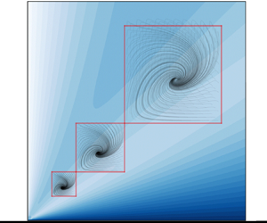
The results obtained for the behaviour of a particle in Stokes flow near a semi-infinite right corner can be applied to improve the one-way coupled particle motion in a closed flow at a finite Reynolds number. This is demonstrated by considering the particle motion in a two-dimensional incompressible flow in a two-sided lid-driven square cavity (Albensoeder, Kuhlmann & Rath Reference Albensoeder, Kuhlmann and Rath2001) as sketched in figure 8. The approach is demonstrated using a variant of the Maxey–Riley equation for the particle motion in the bulk. Since the Maxey–Riley approximation breaks down near the walls, we introduce extra forces in the Maxey–Riley equation such that the correct particle dynamics is recovered as a wall or a singular corner is approached. Similar approaches have widely been used in the literature to complement the Maxey–Riley equation by dedicated particle–boundary models (Kharlamov, Chára & Vlasák Reference Kharlamov, Chára and Vlasák2008; Yang Reference Yang2010; Agarwal, Rallabandi & Hilgenfeldt Reference Agarwal, Rallabandi and Hilgenfeldt2018; Davies et al. Reference Davies, Débarre, El Amri, Verdier, Richter and Bureau2018; Romanò Reference Romanò2019; Romanò et al. Reference Romanò, Kunchi Kannan and Kuhlmann2019a; Agarwal et al. Reference Agarwal, Chan, Gazzola and Hilgenfeldt2021; Magnaudet & Abbas Reference Magnaudet and Abbas2021).

Figure 8. Sketch of a two-dimensional square cavity within which a global flow is driven by an antisymmetric wall motion (arrows). The motion of a particle is considered when its centroid is located inside the red square which outlines the region of validity of the force and torque coefficients provided by Romanò et al. (Reference Romanò, des Boscs and Kuhlmann2020a). In units of the non-dimensional particle radius  $a=a_{p}/L$ the square has a size $a\times a$ and a distance $a$ from both walls, where $L$ is the cavity height. The particle is shown for the case when its centroid is located at its maximum distance, admitted by Romanò et al. (Reference Romanò, des Boscs and Kuhlmann2020a), from the lower left corner. $U_{gL}$ is the settling velocity based on the length L instead of $a_p$.
In the present approach the extra forces near the boundary are based on the fit provided by Romanò et al. (Reference Romanò, des Boscs and Kuhlmann2020a) which takes into account the exact solutions and the asymptotic lubrication theory for a particle moving towards/away from a wall. Therefore, the correction to the Maxey–Riley equation is expected to be valid not only in the strict corner region within which the fit was made (red square in figure 8), but also farther away from the corner when the particle approaches one of the two walls much closer than the other (further details can be found in Romanò et al. (Reference Romanò, des Boscs and Kuhlmann2020a)). By this approach weak inertial effects on the corner attractor can be identified.
The steady flow induced by the moving walls of the cavity must satisfy the Navier–Stokes equations
 $$\begin{gather} \left(\vec u \boldsymbol{\cdot}\boldsymbol{\nabla} \right) \vec u ={-} \boldsymbol{\nabla} p + {\rm \Delta} \vec u, \end{gather}$$
 $$\begin{gather}\boldsymbol{\nabla}\boldsymbol{\cdot} \vec u = 0, \end{gather}$$
where we used a viscous scaling, as in table 1, but with the relevant length scale given by the width  $L$ of the square cavity instead of the particle radius $a_{p}$. In this scaling the velocity field $\vec u$ must satisfy the boundary conditions
 $$\begin{gather} \vec u (z \pm 1/2) = ({\pm} {Re},0)^{\mathrm{T}}, \end{gather}$$
 $$\begin{gather}\vec u (x \pm 1/2) = \vec 0, \end{gather}$$
where the Reynolds number of the flow is defined as
 \begin{equation} {Re} = \frac{U_L L}{\nu}, \end{equation}
with  $U_L$ the magnitude of the lid velocity. The following analysis will be restricted to moderate Reynolds numbers ( ${Re} \leq 100$), for which the flow is steady and two-dimensional (Albensoeder & Kuhlmann Reference Albensoeder and Kuhlmann2003).
In the limit  ${Re}\to 0$ and with the acceleration of gravity $\vec g = (0,-g)^\text {T}$, a small particle would not find a stationary point near the corners $(x,z)=(0.5,\pm 0.5)$ (on the right-hand side in figure 8). From the analysis reported in § 4.1, an attractor for the particle motion is expected near the corner $(x,z)=(-0.5,-0.5)$, while near $(x,z)=(-0.5,0.5)$ a repeller is expected.
Here we focus on the particle motion near  $(x,z)=(-0.5,-0.5)$ and its approach to the attractor when the Reynolds number is ${Re}=O(1)$. For a small particle Reynolds number $\widehat {{Re}}_{p}\ll 1$ and if the time scale of the particle $\tau _{p}$ is much smaller than that of the fluid, i.e. if $\tau _{p}/\tau _{f} = (a_{p}^2/\nu ) (U_L/L) \ll 1$, the particle motion in the bulk can be modelled by one-way coupling. In this approach the flow field is independent of the presence of the particle and can be computed beforehand. Here we use a simplified version of the Maxey–Riley equation (Maxey & Riley Reference Maxey and Riley1983) as in (Babiano et al. Reference Babiano, Cartwright, Piro and Provenzale2000)
 \begin{equation} \ddot{{\boldsymbol{x}}} = \frac{1}{\varrho+1/2} \left[-\frac{\varrho}{{St}}\left(\dot{{\boldsymbol{x}}}-\vec u \right) + \frac{3}{2}\frac{\textrm{D} \vec u }{\textrm{D} t} - (\varrho -1) \frac{\vec e_z}{{Fr}^{2}_L} \right], \end{equation}
where the Stokes and the Froude numbers based on the length of the side walls are defined by
 \begin{equation} {St} = \frac{2}{9}\varrho a^2,\quad {Fr}_L^2 = \frac{\nu^2}{g L^3}, \end{equation}
and  $a=a_{p}/L$ is the relative particle radius.
The form of the Stokes drag in (4.5) is not correct when the particle moves near the boundaries. In order to incorporate the correct viscous effects on the particle motion near the corner  $(x,z)=(-0.5,-0.5)$, the Stokes part $\vec u_S$ of the total velocity field $\vec u$ is separated by writing
 \begin{equation} \vec u = \vec u_{S} + \vec u', \end{equation}
where  $\vec u'$ is the inertial remainder. The term $(\dot {\vec {x}} - \vec u_{S})$ in the drag force due to the Stokes part $\vec u_{S}$ of the flow, which is contained in $(\dot {{\boldsymbol {x}}} - \vec u )$ of (4.5), is now replaced by the numerical approximation of the correct drag forces acting on the sphere obtained by Romanò et al. (Reference Romanò, des Boscs and Kuhlmann2020a) and used in the previous sections. Taking into account the different scalings used here and in § 3 we obtain
 \begin{align} \ddot{{\boldsymbol{x}}} &= \frac{1}{\varrho+1/2} \left[\frac{\varrho}{{St}}\left(\dot{{\boldsymbol{x}}}\boldsymbol{\cdot}{\boldsymbol{e}}_x {\boldsymbol{F}}^{IIIa} + \dot{{\boldsymbol{x}}}\boldsymbol{\cdot}{\boldsymbol{e}}_z {\boldsymbol{F}}^{IIIb} + {Re} {\boldsymbol{F}}^{VIb} + a {\boldsymbol{F}}^{IIa} \frac{\omega}{2} + \vec u' \right)\phantom{\frac{\textrm{D}}{\textrm{D}}\frac{\varrho -1}{{Fr}^2_L}}\right. \nonumber\\ &\quad \left. + \frac{3}{2}\frac{\textrm{D} \vec u' }{\textrm{D} t} - \frac{\varrho -1}{{Fr}^2_L} \vec e_z \right]. \end{align}
By replacing the Stokes part of the drag force, the rotation rate  $\varOmega _y$ of the particle enters (4.8). Because this quantity is not available through the Maxey–Riley equation (4.5), it is modelled here by $\omega /2$, with $\omega = (\nabla\times\vec u)\cdot\vec e_y$ the vorticity of the total flow.
Note (4.8) is valid only within the region (shown as a red square in figure 8) for which the correlations of Romanò et al. (Reference Romanò, des Boscs and Kuhlmann2020a) have been obtained and within which the particle attractor is located in the Stokes flow limit  $\vec u'\to 0$. It is expected that the attractor can be found in this region also for weakly inertial flow $(\vec u'\ne 0)$ in the framework of approximation (4.8). For all simulations carried out, the local particle Reynolds number is moderate with $\widehat {{Re}}_{p}\lesssim 1$ (see figure 9b below), as required by the Maxey–Riley equation.

Figure 9. (a) Particle trajectories converging towards the corner attractor near  $(x,z)=(-0.5, -0.5)$, and initialised velocity matched on a $31\times 31$ tensor grid defined with the bounds $(\delta _x,\delta _z)\in [0.025,0.975]\times [0.025,0.975]$ for $Re = 100$ and $a= 0.005$, $0.01$ and $0.02$ (solid lines). The colour map corresponds to the non-dimensional flow velocity magnitude. (b) Blue shades indicate the magnitude of the deviation from the Stokes corner flow, while red shading indicates the local particle Reynolds $\widehat {{Re}}_{{p}}$ number computed along every ninth particle trajectory as a function of time.
To be able to simulate particle trajectories using the corner-improved model (4.8), first the total flow field  $\vec u$ is computed in the whole domain $(x,z)\in [-1/2,1/2]\times [-1/2,1/2]$ for ${Re}\in [10^{-4},10^{-2},1,25,50,75,100]$, using the finite element library FEniCS (Alnæs et al. Reference Alnæs, Blechta, Hake, Johansson, Kehlet, Logg, Richardson, Ring, Rognes and Wells2015) and a $200\times 200$ basic mesh which is further refined by reducing the grid spacing by a factor of two at each of the distances $0.05$, $0.01$ and $0.005$ from all walls. The velocity and pressure are discretised using Taylor–Hood elements in which the velocity is approximated by piecewise quadratic polynomials, while the pressure is represented by piecewise linear polynomials. Using the Stokes flow solution (2.3) valid near the corner $(x,z)=(-1/2,-1/2)$ the inertial part of the flow $\vec u'$ near this corner is obtained from (4.7).
To probe the attractor, particles were initiated velocity matched to the flow on a regular  $11\times 11$ grid within $[-1/2+1.025a,-1/2+1.975a]\times [-1/2+1.025a,-1/2+ 1.975a]$, inside the red square in figure 8, and (4.8) was integrated in time using the fourth-order 3/8-rule Runge–Kutta method for different particle radii $a \in [0.02, 0.01, 0.005]$. The relative density is kept constant at $\varrho =1.01$.
Figure 9(a) shows three sets of particle trajectories (lines) for  $a= 0.005$, 0.01 and 0.02, respectively, together with the velocity magnitude of the flow. For a reduced set of trajectories shown in figure 9(b), the saturation of the red colour indicates the local particle Reynolds number $\widehat {{Re}}_{p}=\vert \tilde {{\boldsymbol {U}}} + \tilde {{\boldsymbol {\varOmega }}}\times (\tilde {{\boldsymbol {x}}}_{s} - \tilde {{\boldsymbol {x}}}_{p}) - \tilde {{\boldsymbol {u}}}\vert a_{p}/\nu$ along the particle trajectories together with the magnitude of the inertial remainder (blue).
After a short transient all particles were found to be attracted to the same unique attractor, depending on the particle size and on the Reynolds number  ${Re}$. In the case of $a=0.02$, owing to the larger Stokes number, some particles initialised in the upper part of the seeding region, shown in red in figure 8 and 9(a), briefly leave the region of validity of the model (4.8). To treat the particle motion outside of the strict domain of validity (red square in figure 8) the correlations for $F^{IIIa}$, $F^{IIIb}$, $F^{VIb}$ and $F^{IIa}$ of Romanò et al. (Reference Romanò, des Boscs and Kuhlmann2020a) have been extrapolated slightly beyond the original domain of validity by employing the fit also for $\delta _z>1$. However, very similar results are obtained when abruptly switching from the model of Romanò et al. (Reference Romanò, des Boscs and Kuhlmann2020a) to a particle–boundary interaction which only takes into account forces from the plane stationary and moving walls (Jeffery Reference Jeffery1915; Brenner Reference Brenner1961; Chaoui & Feuillebois Reference Chaoui and Feuillebois2003), not taking into account the entrainment effect of the corner flow. In all cases, however, the fixed point is practically unaffected by the exterior model and the phase portraits near the fixed point are qualitatively equivalent to the one shown in figure 3(a). Therefore, the attraction dynamics predicted under the creeping-flow approximation is robust with respect to the addition of small inertial effects and to the particle–boundary interaction model used outside of the red region. Because all particles of the same kind initialised in one of the red regions are attracted to the same unique attractor, the prediction of the Stokesian attractor can be safely generalised to realisable systems such as the present cavity flow.
The location of the attractor is shown in figure 10 in terms of the displacement  $(\delta _{x,z}-\delta _{x,z}^{St})$ relative to the attractor in Stokes flow $(\delta _x^{St},\delta _z^{St})=(0.418,0.346)$ (see figure 4(a)). The displacements in the $x$ and $z$ direction for different particles sizes and flow Reynolds numbers ${Re}$ nearly collapse on a single curve satisfying
 \begin{equation} \delta_{x,z}-\delta_{x,z}^{St} \approx 0.04408\,{Re}_{p} + 0.00495\,{Re}_{p}^2 , \end{equation}
which asymptotes to  $(\delta _{x,z}-\delta _{x,z}^{St}) \approx 0.044\,{Re}_{p}$ for ${Re}_{p}\to 0$ (dashed line in figure 10), where ${Re}_{p}$ denotes the global particle Reynolds number ${Re}_{p} = a {Re}$. The collapse of all data to the almost linear curve (4.9) indicates that the relevant parameter measuring the displacement is indeed the global particle Reynolds number ${Re}_{p}$ (here ${Re}_{p}\le 2$) and that the position of the attractor is shifted away from the corner under an angle of $\approx 45^\circ$ with respect to the $x$ axis.

Figure 10. Displacements in the  $x$ direction (turquoise) and in the $z$ direction (violet) of the attractor near the corner $(x,z)=(-1/2,-1/2)$ as functions of the global particle Reynolds number and for different particle sizes (symbols). The full line is the quadratic fit (4.9) whose linear part is indicated by the dashed line.
In creeping cavity flow a particle repeller is located near  $(x,z)=(-1/2,1/2)$ (near the upper left-hand corner in figure 8), symmetrically placed with respect to the horizontal cavity midplane ( $z = 0$) to the attractor in the lower left-hand corner. Upon an increase of the particle Reynolds numbers, this symmetry is broken: the bottom left attractor moves away from the corner, whereas the top left repeller moves towards the corner. Preliminary computations indicate the same linear asymptotic scaling of the displacement of the repeller for small particle Reynolds number, albeit with a different sign.
The model (4.8) based on the Maxey–Riley equation predicts the existence and location of the corner attractor also for inertial flow. Based on the results obtained it is expected that the attractor is robust and, for moderate Reynolds numbers, will neither be destroyed by higher-order inertial effects not included in (4.8) nor by the nonlinear interaction of the flow with the particle. Therefore, the attractor should also be observable in experiments. A thorough experimental proof, however, is pending.
5. Discussion and conclusion
The Stokesian dynamics of a freely translating and rotating spherical particle near a right dihedral corner was studied for the case when both walls are sliding tangentially to their planes and the gravitational force acts on the particle in an arbitrary direction. By making use of the quasi-steady approach valid for creeping flows, the particle's translational and rotational velocities were expressed by the forces and torques acting on the particle. Based on the fit functions for the forces and torques provided by Romanò et al. (Reference Romanò, des Boscs and Kuhlmann2020a) for the same set-up, the translational and rotational velocities of the particle could be expressed explicitly. This allowed for an extensive parametric study to determine particle trajectories for more than 180 000 configurations.
We find a non-trivial particle attractor in the  $(x,z)$ plane in the form of a spiral sink detached from the walls for $U_{2}=-1$, $W_{2}\in [-1,0.25]$, $U_g\in [-2.2, -0.7]$ and $\phi _x\in [45^\circ , 90^\circ ]$. The attracting line in the flow field $\vec U$ of the particle results from a stable balance between lift forces on the particle due to the fluid entrained by the sliding walls and the gravitational force directed towards the walls. Far away from the corner, the Stokesian lift decays (in creeping flow a particle near a plane does not experience any lift force) and the particle settles on one of the two walls, depending on $U_g$, $\phi _x$ and its initial location. Owing to the symmetry of the Stokesian flow, corresponding repellers are found by inverting the sign of $W_1$, $U_2$ and $U_g$. As the flow field for dihedral corners (without particles) does not experience abrupt changes of its topology upon a smooth variation of the dihedral angle, we expect our results are robust with respect to small deviations of the corner angle from the $90^\circ$ considered in this study. This expectation is supported by the results of Dauparas & Lauga (Reference Dauparas and Lauga2018), who found that the forces and torques on a particle far from the corner vary smoothly with the dihedral angle.
The particle attractor/repeller cannot be inferred from the velocity field  $\vec u$ of the fluid alone. The velocity of the particle $\vec U$ is strongly influenced by gravity, the strength of which is measured by the settling velocity $U_g$, whereas the fluid flow field $\vec u$ is independent of the gravitational acceleration for isothermal incompressible flows.
Based on the definition of  $U_g$, i.e. $U_g = 2(1-\varrho )g a^3/9\nu ^2$, the range $U_g\in [-2.2, -0.7]$ for heavy particles can be relevant for small particles ( $a\in [10^{-4}, 10^{-3}]$ m) in liquids ( $\nu \sim \in [10^{-6}, 10^{-3}]$ m $^2$ s $^{-1}$), for which several combinations of $a$ and $\nu$ can be found such that $a^3/\nu ^2 = O(1)$ s $^2$ m $^{-1}$ and $(1-\varrho )\approx O(1)$. As discussed further below, cavity and junction flows of characteristic lengths up to a few hundreds micrometres represent optimal set-ups for observing corner particle trapping of micron-sized particles.
Several examples of non-trivial finite-size particle attractors in non-chaotic Stokes flows have been reported in the literature. For instance, Sauma-Pérez et al. (Reference Sauma-Pérez, Johnson, Yang and Mullin2018) studied the emergence of a limit cycle for a particle in a rotating drum. For asymptotically small particle Reynolds numbers the theory predicts equilibrium positions resulting from the balance between gravitational, history, inertial forces and Stokes drag. However, owing to the finite-size of the particle, the particle trajectory undergoes a Hopf bifurcation which leads to a stable limit cycle whose size depends on the particle Reynolds number. This non-trivial attractor relates to the finite-size effects in the bulk. Other non-trivial limit cycles are reported for cavity flows (either shear- or lid-driven), where the limit cycle results from a balance between particle inertia and particle–boundary interaction due to the finite particle size. Examples of such limit cycles are reported in Romanò & Kuhlmann (Reference Romanò and Kuhlmann2016), Romanò et al. (Reference Romanò, Kuhlmann, Ishimura and Ueno2017) and Romanò & Kuhlmann (Reference Romanò and Kuhlmann2017). Similar non-trivial limit cycles have recently been reported by Romanò (Reference Romanò2021), where inertial and Coriolis forces are balanced by particle–boundary interactions leading to particle limit cycles in a confined periodically rotating flow. The present study does complement the current literature by demonstrating that particle attractors/repellers exist in two-sided lid-driven cavities near two of the four corners as a result of a balance between gravitational settling and flow entrainment due to the finite particle size.
Apart from closed cavity flows as the one presented in § 4.4, similar corner attractors are expected for microfluidic set-ups, such as, for example, a T-junction used as a flow splitter. In this case, the midplane would be equivalent to a free surface playing the role of a sliding wall, with the difference that the velocity would increase radially from the stagnation line rather than being constant along the driving boundary. In such a set-up, the corner attractor can be observed near the wall at the midplane of symmetry (see figure 3 of Chan, Haward & Shen (Reference Chan, Haward and Shen2018)). Another related set-up is a channel flow past an open microcavity (groove). The flow inside such cavity is driven by the shear layer formed between the channel flow and the recirculating flow inside the cavity. A particle clustering corresponding to our corner attractor has been experimentally observed by Hur, Mach & Di Carlo (Reference Hur, Mach and Di Carlo2011) right before the complete release of particles in the channel. Another example of particle clustering near a corner with a driving surface has been experimentally observed for D-junctions by Volpe et al. (Reference Volpe, Paiè, Ancona, Osellame, Lugarà and Pascazio2017).
We expect the particle attraction/repulsion mechanism unravelled by our study will have an impact on those microfluidic applications in which the flow can be considered Stokesian and is seeded with non-interacting density-mismatched particles. Our study suggests that the positioning of a particle in a free stationary point can be controlled near a singular corner by the orientation of the device with respect to the gravity vector and by the wall velocities. This provides a novel strategy for corner-cleaning applications in microfluidic devices, where the microscopic chips can easily be inclined. In fact, our parametric study shows no corner attractors are formed beyond specific inclination angles  $\phi _x$ of the walls. Moreover, as the Stokesian flow considered admits repellers as counterpart of the attractors, conditions can be identified for which the corner flow admits a repeller such that particles cannot be attracted to the corner. Finally, based on our point-particle simulations, we demonstrated that the attractors/repellers predicted in a semi-infinite corner can be relevant for mildly inertial flows in realisable geometries such as driven cavities.
Declaration of interests
The authors report no conflict of interest.


 Open access