


1. Introduction
In a turbulent plane Couette flow beyond a certain Reynolds number threshold, streamwise-elongated structures spanning the entire channel can be observed, and they have been validated in both simulations (Bech & Andersson Reference Bech and Andersson1994; Komminaho, Lundbladh & Johansson Reference Komminaho, Lundbladh and Johansson1996; Papavassiliou & Hanratty Reference Papavassiliou and Hanratty1997; Tsukahara, Kawamura & Shingai Reference Tsukahara, Kawamura and Shingai2006; Avsarkisov et al. Reference Avsarkisov, Hoyas, Oberlack and Garcia2014; Pirozzoli, Bernardini & Orlandi Reference Pirozzoli, Bernardini and Orlandi2014; Lee & Moser Reference Lee and Moser2018) and experiments (Bech & Andersson Reference Bech and Andersson1994; Tillmark & Alfredsson Reference Tillmark and Alfredsson1995, Reference Tillmark and Alfredsson1998; Kitoh, Nakabyashi & Nishimura Reference Kitoh, Nakabyashi and Nishimura2005; Kitoh & Umeki Reference Kitoh and Umeki2008).
Despite the many aspects of the flow, it has been observed in direct numerical simulations (DNS) that the large-scale rolls grow in length with increasing Reynolds number (Lee & Moser Reference Lee and Moser2018). As a side effect, this led to the conclusion that very long computational boxes had to be used for running turbulent Couette flow (Avsarkisov et al. Reference Avsarkisov, Hoyas, Oberlack and Garcia2014; Lee & Moser Reference Lee and Moser2018). In some works, the very large computational costs have been avoided, which led to the fact that the effect of the too-small box was visible to a certain extent even in the mean flow profile (Lee & Moser Reference Lee and Moser2018). Despite the fact that shear flows are governed by the nonlinear Navier–Stokes equations, certain important aspects of shear flows, such as the streamwise-elongated structures of the plane Couette flow, have their roots in linear mechanisms. Linear analyses revealed that for plane Couette flow, the structures that are most excitable are streamwise-constant. This observation has been made for laminar plane Couette flow by Gustavsson (Reference Gustavsson1981), Butler & Farrell (Reference Butler and Farrell1992), Farrell & Ioannou (Reference Farrell and Ioannou1993), Trefethen et al. (Reference Trefethen, Trefethen, Reddy and Driscoll1993) and Jovanović & Bamieh (Reference Jovanović and Bamieh2005), as well as for its turbulent counterpart for which the linear analyses were performed about the mean flow state (see e.g. del Álamo & Jiménez Reference del Álamo and Jiménez2006; Pujals et al. Reference Pujals, García-Villalba, Cossu and Depardon2009; Hwang & Cossu Reference Hwang and Cossu2010a,Reference Hwang and Cossub).
Despite certain linear mechanisms, in turbulent flows, coherent structures can be understood as being permanently forced via convective nonlinear interactions of the fluctuations. Thus the idea was formed to analyse the flow behaviour as the response to a nonlinear intrinsic forcing through a linearised operator, which led to the development of the resolvent analysis. The idea stems from works of Trefethen et al. (Reference Trefethen, Trefethen, Reddy and Driscoll1993), Farrell & Ioannou (Reference Farrell and Ioannou1993) and Jovanović & Bamieh (Reference Jovanović and Bamieh2005), where linear responses of flows to external excitation were studied. The resolvent-based approach has gained sustained interest due to the work of McKeon & Sharma (Reference McKeon and Sharma2010), where all nonlinear terms in the Fourier-transformed Navier–Stokes equations for the perturbations are summarised as an unknown intrinsic forcing, and key features of wall-bounded turbulent flows (Moarref et al. Reference Moarref, Sharma, Tropp and McKeon2013; Sharma & McKeon Reference Sharma and McKeon2013) have been reproduced with it. These are in particular the reproduction of properties, such as a self-similar distribution of energy for small scales near the wall to a large-scale velocity distribution, two-point correlations in medium and high Reynolds number boundary layers (McKeon & Sharma Reference McKeon and Sharma2010), and the necessity of a logarithmic turbulent mean velocity for geometrically self-similar resolvent modes in turbulent channel flows (Moarref et al. Reference Moarref, Sharma, Tropp and McKeon2013), to name only a few. The resolvent analysis approach has been used for opposition control, considering flow control techniques that employ linear control strategies, as investigated in Luhar, Sharma & McKeon (Reference Luhar, Sharma and McKeon2014) for a pipe flow and e.g. for analysing the effect of riblets in turbulent channel flows as done in Chavarin & Luhar (Reference Chavarin and Luhar2020). The resolvent analysis identifies the forcing modes, which are the most responsive and the most receptive response modes of a dynamical system, in an input–output formulation, based on its governing equations (Herrmann et al. Reference Herrmann, Baddoo, Semaan, Brunton and McKeon2021). The response of the plane Couette flow for low Reynolds numbers has been investigated in Hwang & Cossu (Reference Hwang and Cossu2010a). A component-wise analysis uncovering several amplification mechanisms for subcritical transition and investigating the roles of Tollmien–Schlichting waves, oblique waves, and streamwise vortices and streaks using an input–output system analysis can be found in Jovanović & Bamieh (Reference Jovanović and Bamieh2005). Using an input–output analysis for harmonic forcing, Hwang & Cossu (Reference Hwang and Cossu2010b) show once again that the most amplified structures in the plane Couette flow are largely invariant in streamwise direction, while flows with streamwise wavenumbers significantly smaller than the spanwise wavenumber behave very similarly to streamwise independent flows. Illingworth (Reference Illingworth2020) investigated the amplification mechanism for the coherent structures in a streamwise independent plane Couette flow, which is to a great extent encoded in the Orr–Sommerfeld operator alone, independent of the Squire operator. When investigating the resolvent modes using a turbulent mean velocity profile, it has been shown in Symon, Illingworth & Marusic (Reference Symon, Illingworth and Marusic2021) that the energy transferred from streamwise-constant streaks can be predicted satisfactorily by implementing a Cess eddy viscosity profile for channel flows. The resolvent analysis approach can also be used by employing external forces, as may be seen in Vadarevu et al. (Reference Vadarevu, Symon, Illingworth and Marusic2019), where coherent structures containing long streamwise velocity streaks flanked by quasi-streamwise vortices and hairpin vortices evolved from an impulsive body force in a turbulent channel flow. A link from the resolvent analysis to the linear stability theory highlighting the types of amplification mechanisms was emphasised by Symon et al. (Reference Symon, Rosenberg, Dawson and McKeon2018), where the resolvent norm was split into a resonance part and a non-normal part, thus leading to a deeper understanding of pseudo-resonance phenomena.
The present work aims to understand the apparent length dependence of the Couette roll-cells on the Reynolds number, and thus intends to investigate linear amplification mechanisms in plane Couette flow while focusing on small streamwise wavenumbers  $\alpha \rightarrow 0$ and simultaneously high Reynolds numbers $Re \rightarrow \infty$ with the distinguished limit
 \begin{equation} Re_{\alpha}= \lim_{\substack{Re \rightarrow \infty\\ \alpha \rightarrow 0}} Re \, \alpha=O(1). \end{equation}
This leads to large-scale structures by making use of linear stability theory as well as the operator-driven resolvent analysis approach inserting a laminar base velocity profile. The influence of various parameters, such as the Reynolds number  $Re$, the streamwise and spanwise wavenumbers $\alpha$ and $\beta$, and especially $Re_{\alpha }$, is investigated for harmonic forcing with $\omega \in \mathbb {R}$ on the first singular value $\sigma _1$ for the resolvent analysis and the most critical eigenvalues $\omega _{1,i}$ using linear stability theory in order to analyse the amplification mechanism in the plane Couette flow and thus investigate the appearance of coherent structures in it. The concept of $Re_{\alpha }$ is studied for its role as a global and local invariant in the fields of linear stability theory and resolvent analysis, respectively. The significance of such invariants is emphasised in the pioneering work by Oberlack (Reference Oberlack2001), in which Lie symmetries were utilised in the study of turbulence for the first time to derive invariant solutions. These solutions, known as turbulent scaling laws, play a crucial role in understanding the complex dynamics of turbulent flow.
In the present paper, first the governing equations for the plane Couette flow are derived in § 2. In § 3, linear stability theory is applied on the plane Couette flow within the distinguished asymptotic limit  $Re \rightarrow \infty$ and $\alpha \rightarrow 0$ with $Re_{\alpha }=O(1)$, with the motivation for this limit stemming from the results of § 4. The resulting eigenvalue problem, for which a parameter reduction is obtained, is solved in § 3, where § 3 serves as a preparatory step for the resolvent analysis approach in § 4. The resolvent analysis is then applied on the plane Couette flow in § 4, where the singular values and the response modes are compared to the most critical eigenvalue and the eigenfunctions from § 3. Finally, conclusions are drawn in § 5.
2. Dynamical description of the plane Couette flow system
In this section, the general equations of motion to be used in the subsequent analysis are derived. For this, the Navier–Stokes equations are derived for the wall-normal velocity fluctuation  $u_2'$ and wall-normal vorticity fluctuation $\eta _2'$.
2.1. Governing equations
For the analysis to follow, the Navier–Stokes equations will be the basis, i.e.
 \begin{equation} \frac{\partial u_i}{\partial t}+u_j\,\frac{\partial u_i}{\partial x_j}+\frac{\partial p}{\partial x_i}=\nu\,\frac{\partial^2 u_i}{\partial x_k^2}, \quad \frac{\partial u_i}{\partial x_i}=0, \end{equation}
where  $u_i$ refers to the velocity in each spatial direction $x_i$, with $i=1,2,3$, $p$ denotes the pressure, and $\nu$ represents kinematic viscosity. A Reynolds decomposition for the velocities is introduced:
 \begin{equation} u_1=U_1(x_2)+u_1',\quad u_2=u_2', \quad u_3=u_3', \quad p = p', \end{equation}
with  $U_1(x_2)$ representing the base velocity for the plane Couette flow in the streamwise direction, while $u_i'$ and $p'$ respectively refer to the fluctuations of velocity and pressure. Implementing the aforementioned Reynolds decomposition into the Navier–Stokes equations (2.1a,b) and subtracting the momentum equations for the base flow from the Navier–Stokes equations leads to the following system of equations for the fluctuations:
 \begin{align} \frac{\partial u_1'}{\partial t}+U_1(x_2)\,\frac{\partial u_1'}{\partial x_1}+\frac{{\rm d} U_1(x_2)}{{\rm d} x_2}\,u_2'+\frac{\partial p'}{\partial x_1}-\nu\,\frac{\partial^2 u_1'}{\partial x_k^2}=f_1' , \end{align}
 \begin{align} \frac{\partial u_2'}{\partial t}+U_1(x_2)\,\frac{\partial u_2'}{\partial x_1}+\frac{\partial p'}{\partial x_2}-\nu\,\frac{\partial^2 u_2'}{\partial x_k^2}=f_2' , \end{align}
 \begin{align} \frac{\partial u_3'}{\partial t}+U_1(x_2)\,\frac{\partial u_3'}{\partial x_1}+\frac{\partial p'}{\partial x_3}-\nu\,\frac{\partial^2 u_3'}{\partial x_k^2}=f_3', \end{align}
with all the nonlinearities being summarised as an intrinsic forcing term on the right-hand side as
 \begin{equation} f_i'={-}u_j'\,\frac{\partial u_i'}{\partial x_j}+\overline{u_j'\,\frac{\partial u_i'}{\partial x_j}}. \end{equation}
Further, the continuity equation for the fluctuations is given by
 \begin{equation} \frac{\partial u_i'}{\partial x_i}=0. \end{equation}
All velocity fluctuations vanish at both walls, i.e. at  $x_2=\pm 1$, yielding conditions in the form $\begin{pmatrix} u_1' & u_2' & u_3' \end{pmatrix}^{\rm T} (x_1,x_2=\pm 1,x_3)=0$, where all length scales have been non-dimensionalised by the channel half-width $h$. In this work, the linear stability theory is to be compared directly with the resolvent analysis, and for this the laminar base flow forms the basis for both approaches.
Thus the velocity profile for the laminar plane Couette flow is used subsequently as  $U_1(x_2) = A x_2$, which allows an explicit derivation of the analytical solutions for the eigenfunctions of the linear stability theory, where $A$ represents an inverse time scale and at the same time defines the velocity at the wall, i.e. $U_w=\pm A h$. We have also analysed a turbulent mean flow based on DNS data of a turbulent Couette flow, with the key findings remaining qualitatively identical to those obtained from the laminar base flow, albeit exhibiting only a quantitative rescaling in the magnitudes. Consequently, in order to utilise explicit analytical solutions for the eigenfunctions of the linear stability theory, we decided to focus on the laminar base velocity. Non-dimensionalising with $A$ and $h$, the Reynolds number may be defined as
 \begin{equation} Re=\frac{A h^2}{\nu} . \end{equation}
Thus the system (2.3a)–(2.3c) can be rewritten such that the viscosity  $\nu$ can be replaced by ${1}/{Re}$, and the laminar base flow reads $U_1(x_2)=x_2$.
2.2. Wall-normal formulation
In the following, the basic equations (2.3) are rewritten in a wall-normal velocity–vorticity formulation. We obtain the wall-normal form of the Navier–Stokes equations for the fluctuations by taking the Laplacian of (2.3b) as well as the divergence of (2.3), and by taking the curl of (2.3a) and (2.3c), where we have also employed the wall-normal vorticity  $\eta _2'={\partial u_1'}/{\partial x_3}-{\partial u_3'}/{\partial x_1}$. With this, the Navier–Stokes equations for the fluctuations $u_2'$ and $\eta _2'$ read
 \begin{equation} \frac{\partial}{\partial t}\,\Delta u_{2}'+x_2\,\frac{\partial}{\partial x_1} \Delta u_{2}'-\frac{1}{Re}\,\Delta^2 u_{2}'={-}\frac{\partial^2 f_1'}{\partial x_1\,\partial x_2}-\frac{\partial^2 f_2'}{\partial x_1^2}+\frac{\partial^2 f_2'}{\partial x_3^2}-\frac{\partial^2 f_3'}{\partial x_2\,\partial x_3} \end{equation}
and
 \begin{equation} \frac{\partial \eta_{2}'}{\partial t}+\frac{\partial u_{2}'}{\partial x_3}+x_2\,\frac{\partial \eta_{2}'}{\partial x_1}-\frac{1}{Re}\,\Delta \eta_2'=\frac{\partial f_1'}{\partial x_3}-\frac{\partial f_3'}{\partial x_1}. \end{equation}
Solid wall boundary conditions for the wall-normal formulation are Dirichlet boundary conditions for  $u_2'$ and $\eta _2'$ as well as the Neumann boundary condition for $u_2'$, that is, $\begin{pmatrix} u_2' & { \partial u_2'}/{\partial x_2} & \eta _2' \end{pmatrix}^{\rm T} (x_1,x_2=\pm 1,x_3)=0$. For the further analysis below, we employ a Fourier decomposition in the streamwise and spanwise directions as well as in time to obtain
 $$\begin{gather} u_{i}'=\tilde{u}_{i}'(x_2)\exp({\mathrm{i}(\alpha x_1+\beta x_3-\omega t)}), \end{gather}$$
 $$\begin{gather}\eta_{2}'=\tilde{\eta}_{2}'(x_2)\exp({\mathrm{i}(\alpha x_1+\beta x_3-\omega t)}), \end{gather}$$
with  $\alpha \in \mathbb {R}$ and $\beta \in \mathbb {R}$ being the streamwise and spanwise wavenumbers, while $\omega \in \mathbb {C}$ represents the frequency of the fluctuations, which leads to the wall-normal velocity–vorticity formulation of the Navier–Stokes equations for the fluctuations:
 \begin{align} &{-\mathrm{i}}\omega\left((\alpha^2+\beta^2)\tilde{u}_{2}'-\frac{{\rm d}^2 \tilde{u}_{2}'}{{\rm d} x_2^2}\right)+\mathrm{i}\alpha x_2\left((\alpha^2+\beta^2)\tilde{u}_{2}'-\frac{{\rm d}^2 \tilde{u}_{2}'}{{\rm d} x_2^2}\right)\nonumber\\ &\quad -\frac{1}{Re}\left(\frac{{\rm d}^4 \tilde{u}_{2}'}{{\rm d} x_2^4}-2(\alpha^2+\beta^2)\frac{{\rm d}\tilde{u}_{2}'}{{\rm d} x_2^2}+(\alpha^2+\beta^2)^2 \tilde{u}_{2}'\right)\nonumber\\ &\qquad={-}\mathrm{i} \alpha\,\frac{{\rm d} \tilde{f}_1'}{{\rm d} x_2}+(\alpha^2 -\beta^2 )\tilde{f}_2'-\mathrm{i}\beta\,\frac{{\rm d} \tilde{f}_3'}{{\rm d} x_2}, \end{align}
 \begin{align} &-\mathrm{i} \omega \tilde{\eta}_{2}'+ \mathrm{i} \alpha x_2 \tilde{\eta}_{2}'+\mathrm{i} \beta \tilde{u}_2'-\frac{1}{Re}\left(\frac{{\rm d}^2 \eta_{2}'}{{\rm d} x_2^2}-(\alpha^2+\beta^2) \tilde{\eta}_{2}'\right)=\mathrm{i} \beta \tilde{f}_1'-\mathrm{i} \alpha \tilde{f}_3', \end{align}
with the continuity equation
 \begin{equation} \mathrm{i} \alpha \tilde{u}_1'+\frac{{\rm d} \tilde{u}_2'}{{\rm d} x_2}+\mathrm{i} \beta \tilde{u}_3'=0, \end{equation}
where  $\tilde {f}_i =(-u_j' ({\partial u_i'}/{\partial x_j}) )_{\boldsymbol {k}}$ denotes the Fourier transformed nonlinear forcing term corresponding to the generalised wavenumber vector $\boldsymbol {k}=\begin{pmatrix} \alpha & \beta & \omega \end{pmatrix}^{\rm T}$. All velocity fluctuations $\tilde {u}_i'$ are generated from the wall-normal fluctuations $\tilde {u}_2'$ and $\tilde {\eta }_2'$ using the continuity equation (2.13), since $\tilde {u}_2'$ and $\tilde {\eta }_2'$ are considered as known quantities. Introducing $k=\sqrt {\alpha ^2+\beta ^2}$, the velocity fluctuations $\tilde {u}_i'$ are then given by
 \begin{equation}
\begin{pmatrix} \tilde{u}_1'\\[2pt] \tilde{u}_2'\\
\tilde{u}_3'\end{pmatrix}=\boldsymbol{\mathsf{C}}\begin{pmatrix}
\tilde{u}_2'\\ \tilde{\eta}_2' \end{pmatrix},
\quad \mathrm{with} \ \boldsymbol{\mathsf{C}}=\dfrac{1}{k^2}
\begin{pmatrix} \mathrm{i} \alpha\,\dfrac{{\rm d}}{{\rm d}
x_2} & -\mathrm{i} \beta \\ k^2 & 0 \\ \mathrm{i} \beta\, \dfrac{{\rm
d}}{{\rm d} x_2} & \mathrm{i} \alpha \end{pmatrix}.
\end{equation}
\begin{equation}
\begin{pmatrix} \tilde{u}_1'\\[2pt] \tilde{u}_2'\\
\tilde{u}_3'\end{pmatrix}=\boldsymbol{\mathsf{C}}\begin{pmatrix}
\tilde{u}_2'\\ \tilde{\eta}_2' \end{pmatrix},
\quad \mathrm{with} \ \boldsymbol{\mathsf{C}}=\dfrac{1}{k^2}
\begin{pmatrix} \mathrm{i} \alpha\,\dfrac{{\rm d}}{{\rm d}
x_2} & -\mathrm{i} \beta \\ k^2 & 0 \\ \mathrm{i} \beta\, \dfrac{{\rm
d}}{{\rm d} x_2} & \mathrm{i} \alpha \end{pmatrix}.
\end{equation}2.3. Distinguished asymptotic analysis
The present focus is on large-scale streamwise coherent structures, which are observed to occur for high Reynolds number plane Couette flow, which admits very weak streamwise variation as may e.g. be taken from Hwang & Cossu (Reference Hwang and Cossu2010b). Hence we intend to analyse the asymptotic limits of  $\alpha \rightarrow 0$ and $Re \rightarrow \infty$, which are the key parameters to observe coherent channel-wide structures. Yalcin, Turkac & Oberlack (Reference Yalcin, Turkac and Oberlack2021) studied this coupled limiting case for an asymptotic suction boundary layer in great detail, where the actual analysis was based on the Orr–Sommerfeld equation and led to a rather generic result. They concluded that separate limiting procedures were of little value, whereas the distinguished limit (DL)
 \begin{equation} Re_{\alpha}= \lim_{\substack{Re \rightarrow \infty\\ \alpha \rightarrow 0}} Re \, \alpha=O(1) \end{equation}
led to a self-consistent asymptotic, and a global minimum for  $Re_{\alpha }$ could be calculated. The analysis can be extended for the present case. For this purpose, the corresponding expansion (2.15) is inserted into (2.11)–(2.12), and all terms of order O( $\alpha ^n$) with $n>1$ have been neglected in the subsequent equations.
3. Linear stability theory
In this section, we want to investigate plane Couette flow within the DL using linear stability theory, where the interest in this limit was further motivated from the results shown in figure 4 in § 4, where only structures for this limit are sustainably amplified. This section is meant to be understood as a preparatory step for the resolvent analysis approach in § 4.
3.1. Orr–Sommerfeld and Squire equations
The Orr–Sommerfeld and Squire equations are obtained by applying the expansion (2.15) and setting the right-hand sides of (2.11) and (2.12) to 0 due to considering only small fluctuations  $\tilde {u}_2'$ and $\tilde {\eta }_2'$ of order $O(\epsilon )$ with $\epsilon \ll 1$, leading to negligible nonlinearities $\tilde {f}_i'$ of order $O(\epsilon ^2)$. Furthermore, we observe that terms of order ${\omega }/{\alpha }$ prevail, hence a low-frequency assumption is implied, as in Yalcin et al. (Reference Yalcin, Turkac and Oberlack2021):
 \begin{equation} \omega=\omega_1 \alpha + O(\alpha^2), \end{equation}
resulting in the leading-order versions of the Orr–Sommerfeld and Squire equations given as
 \begin{equation} {-\mathrm{i}}\omega_1\,Re_{\alpha} \left(\beta^2 \tilde{u}_2'- \frac{{\rm d}^2 \tilde{u}_2'}{{\rm d} x_2^2}\right)+\mathrm{i}\,Re_{\alpha}\,x_2 \left( \beta^2 \tilde{u}_2'- \frac{{\rm d}^2 \tilde{u}_2'}{{\rm d} x_2^2}\right)+\frac{{\rm d}^4 \tilde{u}_2'}{{\rm d} x_2^4}-2\beta^2\,\frac{{\rm d}^2 \tilde{u}_2'}{{\rm d} x_2^2}+\beta^4 \tilde{u}_2'=0 \end{equation}
and
 \begin{equation} {-\mathrm{i}}\omega_1\,Re_{\alpha}\,\tilde{\eta}_2'+ \mathrm{i}\,Re_{\alpha}\,x_2 \tilde{\eta}_2'+ \mathrm{i} \beta\,\frac{Re_{\alpha}}{\alpha}\,\tilde{u}_2'-\frac{{\rm d}^2 \tilde{\eta}_2'}{{\rm d} x_2^2}+\beta^2 \tilde{\eta}_2'=0. \end{equation}
The reduced Orr–Sommerfeld equation (3.2) is dependent only on the newly introduced variable  $Re_{\alpha }$ due to the low-frequency assumption, whereas the Squire equation (3.3) still contains $\alpha$. Thus the wall-normal velocity fluctuation $\tilde {u}_2'$ has to be of order $O(\alpha )$ compared to the wall-normal vorticity fluctuation $\tilde {\eta }_2'$ so that all the terms are of the same order. This is also supported by the observation of Schmid & Henningson (Reference Schmid and Henningson2001), that in particular, the wall-normal vorticity in an Orr–Sommerfeld mode is typically orders of magnitude larger than the wall-normal velocity. Thus we set $\tilde {u}_2=\alpha \tilde {u}_{2,\alpha }$, where $\alpha$ is used to rescale $\tilde {u}_{2}$. By this assumption, $\alpha$ formally vanishes in the Squire equation (3.3) as well, leading to the modified Orr–Sommerfeld and Squire equations
 $$\begin{gather} -\mathrm{i} \omega_1\,Re_{\alpha} \left(\beta^2 \tilde{u}_{2,\alpha}'- \frac{{\rm d}^2 \tilde{u}_{2,\alpha}'}{{\rm d} x_2^2}\right)+\mathrm{i}\,Re_{\alpha}\,x_2 \left( \beta^2 \tilde{u}_{2,\alpha}'- \frac{{\rm d}^2 \tilde{u}_{2,\alpha}'}{{\rm d} x_2^2}\right)\nonumber\\ + \frac{{\rm d}^4 \tilde{u}_{2,\alpha}'}{{\rm d} x_2^4}-2\beta^2\,\frac{{\rm d}^2 \tilde{u}_{2,\alpha}'}{{\rm d} x_2^2} +\beta^4 \tilde{u}_{2,\alpha}'=0 \end{gather}$$
and
 \begin{equation} {-\mathrm{i}}\omega_1\,Re_{\alpha}\,\tilde{\eta}_2'+ \mathrm{i}\,Re_{\alpha}\,x_2 \tilde{\eta}_2'+ \mathrm{i} \beta\,Re_{\alpha}\,\tilde{u}_{2,\alpha}'-\frac{{\rm d}^2 \tilde{\eta}_2'}{{\rm d} x_2^2}+\beta^2 \tilde{\eta}_2'=0, \end{equation}
where a parameter reduction in both (3.4) and (3.5) using  $Re_{\alpha }$ is obtained. Thus in the linear stability theory, $Re_{\alpha }$ affects the system of the plane Couette flow globally within the DL of $Re \rightarrow \infty$ and $\alpha \rightarrow 0$, where it can be seen that invariant solutions can be found independent of both $Re$ and $\alpha$ as long as the product $Re_{\alpha }$ within the DL remains the same. This supports the observation in DNS studies of growing streamwise lengths with the Reynolds number (Lee & Moser Reference Lee and Moser2018) for invariant structures as $\alpha$ has to decrease for an increasing $Re$ for $Re_{\alpha }$ to remain constant.
3.2. Derivation of an eigenvalue problem
The solution for the rescaled wall-normal velocity fluctuation  $\tilde {u}'_{2,\alpha }$ is obtained analytically from the modified Orr–Sommerfeld equation (3.4) in terms of integrals of Airy functions $\text {Ai}(z)$ and $\text {Bi}(z)$ using Maple 2020 as
 \begin{align} \tilde{u}'_{2,\alpha}&={C}_1\,{\rm e}^{\beta x_2} +{C}_2\,{\rm e}^{\beta x_2} \int_{{-}1}^{x_2} {\rm e}^{{-}2\beta x_2} \,{\rm d} x_2\nonumber\\ &\quad +{C}_3\left(\frac{{\rm e}^{\beta x_2}}{2\beta}\,E_1(Re_{\alpha},\beta,\omega_1,x_2) -\frac{{\rm e}^{-\beta x_2}}{2\beta}\,E_2(Re_{\alpha},\beta,\omega_1,x_2)\right) \nonumber\\ &\quad +{C}_4\left(\frac{{\rm e}^{\beta x_2}}{2\beta}\,E_3(Re_{\alpha},\beta,\omega_1,x_2) -\frac{{\rm e}^{-\beta x_2}}{2\beta}\,E_4(Re_{\alpha},\beta,\omega_1,x_2) \right) , \end{align}
with
 \begin{equation} E_j(Re_{\alpha},\beta,\omega_1,x_2)=\int _{{-}1}^{x_2} {\rm e}^{({-}1)^j\beta x_2}\,\text{Ai}\left((-\mathrm{i})^{1/3}\,Re_{\alpha}^{{-}2/3}\left(Re_{\alpha} \left(\omega_1-x_2\right)+\mathrm{i} \beta^2\right)\right) {\rm d} x_2, \end{equation}
for  $j=1,2$, and
 \begin{equation} E_l(Re_{\alpha},\beta,\omega_1,x_2)=\int _{{-}1}^{x_2} {\rm e}^{({-}1)^l\beta x_2}\, \text{Bi}\left((-\mathrm{i})^{1/3}\,Re_{\alpha}^{{-}2/3}\left(Re_{\alpha} \left(\omega_1-x_2\right)+\mathrm{i} \beta^2\right)\right) {\rm d} x_2, \end{equation}
for  $l=3,4$.
The Dirichlet and Neumann boundary conditions for the rescaled wall-normal velocity fluctuation  $\begin{pmatrix} \tilde {u}_{2,\alpha }' & { \partial \tilde {u}_{2,\alpha }'}/{\partial x_2} \end{pmatrix}^{\rm T} (x_1,x_2=\pm 1,x_3)=0$ may be written in homogeneous matrix form as
 \begin{equation} \boldsymbol{\mathsf{A}}(Re_{\alpha},\beta,\omega_1) \boldsymbol{\cdot} \boldsymbol{\mathsf{C}}=\boldsymbol{0}, \end{equation}
where the solution for the wall-normal eigenfunction  $\tilde {u}_{2,\alpha }$ in (3.6) as well for its derivative ${\partial \tilde {u}_{2,\alpha }}/{\partial x_2}$ (see Appendix A) is used with $\boldsymbol{\mathsf{C}}=\begin{pmatrix} {C}_1 & {C}_2 & {C}_3 & {C}_4 \end{pmatrix}^{\rm T}$. The elements of the matrix $\boldsymbol{\mathsf{A}}$ represent the respective coefficients for the Dirichlet and Neumann boundary conditions and are to be taken from Appendix A as well. For a non-trivial solution to exist, the determinant of $\boldsymbol{\mathsf{A}}(Re_{\alpha },\beta,\omega _1)$ has to vanish, yielding the dispersion relation
 \begin{equation} \text{det}(\boldsymbol{\mathsf{A}}(Re_{\alpha},\beta,\omega_1))=A_{14} A_{33} - A_{13} A_{34} = 0. \end{equation}
For a good initial guess for the eigenvalues, a Chebyshev collocation point based method is applied to (3.4), for which the package by Schmid & Henningson (Reference Schmid and Henningson2001) was modified for the problem at hand in order to solve for the eigenvalues  $\omega _1$ numerically. The sole employment of the spectral collocation method based on the Chebyshev polynomials is not enough to acquire physical spectra due to the existence of spurious modes. Thus in order to eliminate these spurious modes and to increase the accuracy of higher modes in the spectra, all eigenvalues obtained numerically were subsequently refined iteratively by evaluating the complex nonlinear dispersion relation (3.9), in which the eigenvalues $\omega _1$ occur nonlinearly due to the nature of the entries $A_{13}, A_{14}, A_{33}, A_{34}$, which can be seen in Appendix A even though one must note that the original modified Orr–Sommerfeld equation (3.4) used for the derivation of the dispersion relation (3.9) is linear in both the eigenvalues $\omega _{1}$ and rescaled eigenfunctions $u_{2,\alpha }'$. The eigenvalues obtained by the Chebyshev collocation method were employed as starting points in a nonlinear root finder with Maple 2020. The iteration was halted when the residual of the eigenvalue problem (3.9) reached a threshold of $O(10^{-60})$.
The most critical eigenvalue obtained numerically,  $\omega {}_{1,{i}}=\text {Imag}(\omega _1)$, is shown over $\beta$ for $Re_{\alpha }=1,1.5,5$ in figure 1(a), and over $Re_{\alpha }$ for $\beta =1,1.5,2$ in figure 1(b). It can be seen that for e.g. $Re_{\alpha }=1$, the most critical eigenvalue obtained numerically, $\omega {}_{1,{i}}$, over $\beta$ reaches its maximum for $\beta _{max}=1.2$. For larger values of $Re_{\alpha }$, the most critical eigenvalue obtained numerically, $\omega {}_{1,{i}}$, converges towards the neutral stability boundary at $\omega _{1,{i}}=0$. To analyse the coherent structures obtained from the linear stability theory, it is necessary to solve for the wall-normal eigenfunctions $\tilde {u}_{2,\alpha }'$ and $\tilde {\eta }_2'$ first. To solve for the wall-normal vorticity fluctuation $\tilde {\eta }_2'$ analytically using Maple 2020, the modified Squire equation (3.5) can be used, resulting in
 \begin{align} \tilde{\eta}'_2&={C}_5\,\text{Ai}\left(Z(x_2)\right)+{C}_6\,\text{Bi}\left(Z(x_2)\right) +\frac{\mathrm{i} {\rm \pi}\,Re_{\alpha}\,\beta }{(-{\rm i}\, Re_{\alpha})^{1/3}}\left[\text{Ai}\left(Z(x_2)\right)\int_{{-}1}^1 \text{Bi}\left(Z(x_2)\right) \tilde{u}'_{2,\alpha}\,{\rm d} x_2\right.\nonumber\\ &\left.\quad{}-\text{Bi}\left(Z(x_2)\right) \int_{{-}1}^1 \text{Ai}\left(Z(x_2)\right) \tilde{u}'_{2,\alpha}\,{\rm d} x_2\right], \end{align}
with  $Z(x_2)=(-\mathrm {i})^{1/3}\,Re_{\alpha }^{-2/3}(Re_{\alpha }\,(\omega _1-x_2)+\mathrm {i} \beta ^2)$. The calculation for the constants ${C}_i$ within the analytical solutions for both $\tilde {u}_{2,\alpha }'$ in (3.6) and $\tilde {\eta }_2'$ in (3.10) using the boundary conditions $\begin{pmatrix} \tilde {u}_2' & { \partial \tilde {u}_2'}/{\partial x_2} & \tilde {\eta }_2' \end{pmatrix}^{\rm T} (x_1,x_2=\pm 1,x_3)=0$ is shown in Appendix A. The streamwise and spanwise velocity fluctuations $\tilde {u}'_1$ and $\tilde {u}'_3$ can be obtained using the continuity equation (2.14), resulting in
 $$\begin{gather} \tilde{u}'_1={-}\frac{\mathrm{i}}{\beta}\,\tilde{\eta}_2', \end{gather}$$
 $$\begin{gather}\tilde{u}'_3=\frac{\mathrm{i}}{\beta}\,\alpha\tilde{u}_{2,\alpha}'+\frac{\mathrm{i}}{\beta}\,\alpha \tilde{\eta}_2' . \end{gather}$$
Inserting (3.6) into  $\tilde {u}_2'=\alpha \tilde {u}_{2,\alpha }$, one can see that $\alpha$ acts as a magnitude amplifier in the wall-normal velocity fluctuation $\tilde {u}_2'$, while its qualitative behaviour is dependent only on $Re_{\alpha }$. From (3.10), it can be seen that the wall-normal vorticity fluctuation $\tilde {\eta }_2'$ depends only on $Re_{\alpha }$ in both its qualitative and quantitative behaviour. From (3.11a), one can see that the streamwise velocity fluctuation $\tilde {u}_1'$ thus is also dependent only on $Re_{\alpha }$. Furthermore in (3.11b), one can rewrite $\tilde {u}_3'=\alpha \tilde {u}_{3,\alpha }'$, with $\tilde {u}_{3,\alpha }'=({\mathrm {i}}/{\beta })\tilde {u}_{2,\alpha }'+({\mathrm {i}}/{\beta }) \tilde {\eta }_2'$, thus $\alpha$ also acts only as a magnitude amplifier for $\tilde {u}_3'$, while its qualitative behaviour is dependent only on $Re_{\alpha }$. Figure 2 shows the analytically obtained eigenfunctions for $\tilde {u}_1'$, $\tilde {u}_{2,\alpha }$ and $\tilde {u}_{3,\alpha }$ for $Re_{\alpha }=1$ and $\beta =2$. The most critical eigenvalue was solved for using (3.9), and was found at $\omega _1=-10.1590\,\mathrm {i}$.

Figure 1. The most critical eigenvalue obtained numerically,  $\omega {}_{1,{i}}$: (a) over $\beta$ for $Re_{\alpha }=1,1.5,5$; and (b) over $Re_{\alpha }$ for $\beta =1,1.5,2$.

Figure 2. The analytically obtained eigenfunctions  $\tilde {u}_1'$, $\tilde {u}_{2,\alpha }'$, $\tilde {u}_{3,\alpha }'$ for $\beta =2$, $Re_{\alpha }=1$, for the most critical eigenvalue $\omega _1=-10.1590\,\mathrm {i}$, over the wall-normal direction $x_2$. Solid lines represent the real part of the solution, with dotted lines representing the imaginary part of the eigenfunctions.
3.3. Influence of  $Re_{\alpha }$ on the streamwise fluctuation structures

The streamwise fluctuations are shown over the spanwise direction  $x_3$ and wall-normal direction $x_2$ by plotting the real part of the product of the complex-valued streamwise eigenfunction with the Fourier decomposition in spanwise direction with $\operatorname {Re}(\tilde {u}_1'(x_2)\,{\rm e}^{\mathrm {i}\beta x_3})$ for $\beta =2$, $Re_{\alpha }=1$, $\omega _1=-10.1590\,\mathrm {i}$ (figure 3a), $\beta =2$, $Re_{\alpha }=5$, $\omega _1=-2.0507\,\mathrm {i}$ (figure 3b), and $\beta =2$, $Re_{\alpha }=10$, $\omega _1=-1.0553\, \mathrm {i}$ (figure 3c). Here, the most critical obtained eigenvalues for a given parameter combination $(\beta,Re_{\alpha })$ obtained from (3.9) were used.

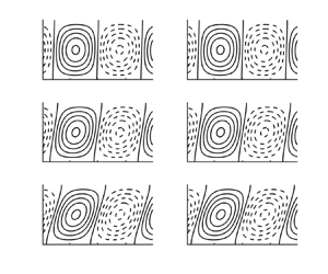
Figure 3. Streamwise fluctuations over the spanwise direction  $x_3$ and wall-normal direction $x_2$ for (a) $\beta =2$, $Re_{\alpha }=1$, $\omega _1=-10.1590\,\mathrm {i}$, (b) $\beta =2$, $Re_{\alpha }=5$, $\omega _1=-2.0507\,\mathrm {i}$, and (c) $\beta =2$, $Re_{\alpha }=10$, $\omega _1=-1.0553\,\mathrm {i}$. Solid lines represent fluctuations with a positive sign, while dashed lines represent fluctuations with a negative sign.
An increasing value of  $Re_{\alpha }$ causes a stronger inclination of the structures in the direction of the propagating waves in the wall-normal and spanwise plane due to the Orr mechanism. Since for $\alpha \neq 0$, the waves are no longer propagating in the streamwise direction alone, an inclination can be observed within the wall-normal and spanwise directions due to the Orr mechanism. A reflexion symmetry break for a sign change in $\beta$ is observed in the inclination direction of the structures.
Since the eigenvalues  $\omega _1$ and the eigenfunctions in the streamwise direction are dependent only on $Re_{\alpha }$, in order to obtain constant structures for growing Reynolds numbers, the streamwise wavenumber has to decrease, agreeing with the observations made in Lee & Moser (Reference Lee and Moser2018) about increasing length of the streamwise rolls with the Reynolds number.
4. Resolvent analysis
In this section, we are applying the resolvent analysis in the DL used in § 3 on the plane Couette flow in order to connect the linear stability theory with the resolvent analysis, where we aim to compare the results of both approaches regarding the optimal wavenumber combination for the coherent structures, the energy and the appearance of these structures and the Reynolds-number-induced growth of these large-scale rolls obtained from both approaches with each other. For this, it is necessary to rewrite (2.11) and (2.12) in an input–output system by reformulating them into the matrix system
 \begin{equation} \mathrm{i} \omega \tilde{\boldsymbol{q}}'=\boldsymbol{\mathsf{L}} \tilde{\boldsymbol{q}}'+\boldsymbol{\mathsf{B}} \tilde{\boldsymbol{f}}', \end{equation}
with the output vector  $\tilde {\boldsymbol {q}}'=\left (\begin{smallmatrix} \tilde {u}_2'\\ \tilde {\eta }_2' \end{smallmatrix}\right )$ and the input vector $\tilde {\boldsymbol {f}}'=\begin{pmatrix} \,\tilde {f}_1'& \tilde {f}_2'& \tilde {f}_3' \end{pmatrix}^{\rm T}$. Here, $\boldsymbol{\mathsf{L}}$ represents the Orr–Sommerfeld and Squire operator, i.e.
 \begin{equation} \boldsymbol{\mathsf{L}}=\boldsymbol{\mathsf{M}}^{{-}1}\begin{pmatrix} -\mathrm{i}\,Re\,\alpha x_2 \left(\dfrac{{\rm d}^2}{{\rm d} x_2^2}-k^2\right)+\dfrac{{\rm d}^4}{{\rm d} x_2^4}-2 k^2\,\dfrac{{\rm d}^2}{{\rm d} x_2^2}+k^4 & 0 \\ - \mathrm{i}\,Re\,\beta & - \mathrm{i}\,Re\, \alpha x_2+\dfrac{{\rm d}^2}{{\rm d} x_2^2}-k^2 \end{pmatrix}, \end{equation}
where the mass matrix  $\boldsymbol{\mathsf{M}}$ reads
 \begin{equation} \boldsymbol{\mathsf{M}}=\begin{pmatrix} Re \left( \dfrac{{\rm d}^2}{{\rm d} x_2^2}-k^2 \right) & 0 \\[2pt] 0 & Re \end{pmatrix}, \end{equation}
and the matrix  $\boldsymbol{\mathsf{B}}$ is given as
 \begin{equation} \boldsymbol{\mathsf{B}}=\boldsymbol{\mathsf{M}}^{{-}1}\begin{pmatrix} -\mathrm{i}\,Re\,\alpha\,\dfrac{{\rm d}}{{\rm d} x_2} & - Re\,k^2 & -\mathrm{i} \beta\,Re\,\dfrac{{\rm d}}{{\rm d} x_2} \\[2pt] \mathrm{i}\,Re\,\beta & 0 & -\mathrm{i}\,Re\,\alpha \end{pmatrix}. \end{equation}
In a final step, we may rewrite (4.1), by introducing the resolvent matrix  $\boldsymbol{\mathsf{H}}$ and making use of the unit matrix $\boldsymbol{\mathsf{I}}$, as
 \begin{equation} \tilde{\boldsymbol{q}}'=(\mathrm{i} \omega \boldsymbol{\mathsf{I}}-\boldsymbol{\mathsf{L}})^{{-}1} \boldsymbol{\mathsf{B}}\tilde{\boldsymbol{f}}'=(\mathrm{i} \omega \boldsymbol{\mathsf{I}}-\boldsymbol{\mathsf{L}})^{{-}1} \tilde{\boldsymbol{f}}_B'=\boldsymbol{\mathsf{H}}\tilde{\boldsymbol{f}}_B'. \end{equation}
4.1. Singular value decomposition
The goal of the resolvent analysis is to identify the dominant directions along which  $\tilde {\boldsymbol {f}}_B'$ can be most amplified through the resolvent operator $\boldsymbol{\mathsf{H}}$ to form the corresponding responses in $\tilde {\boldsymbol {q}}'$. By using a singular value decomposition on the resolvent operator $\boldsymbol{\mathsf{H}}$, one can obtain the most amplified response and forcing modes for given wavenumbers $\alpha, \beta, \omega$ and Reynolds numbers $Re$. Response modes can be considered to represent the coherent structures that occur in the plane Couette flow, where only the knowledge of the base velocity profile $U_1(x_2)=x_2$ has been employed. Applying a singular value decomposition rewrites the resolvent matrix as $\boldsymbol{\mathsf{H}}=\boldsymbol {U} \boldsymbol {S} \boldsymbol {V}^{\rm T}$. In this formulation, $\boldsymbol{\mathsf{S}}$ represents a diagonal matrix with the singular values $\sigma _n=\sqrt {\lambda _n}$ in decreasing order on its diagonal, where $\lambda _n$ are the eigenvalues of $\boldsymbol {H}^{\rm T}\boldsymbol{\mathsf{H}}$. Therefore, $\sigma _1$ represents the maximum singular value on a given set of parameters. The matrix $\boldsymbol{\mathsf{V}}^{\rm T}$ contains the forcing modes ${\varPhi }_j$, while $\boldsymbol{\mathsf{U}}$ contains the respective response modes ${\varPsi }_j$. Both sets of singular vectors are guaranteed to form an orthonormal basis and are ranked according to their singular values. Thus the resolvent operator can be rewritten as
 \begin{equation} \boldsymbol{\mathsf{H}}=\sum_{j=1}^{\infty} {\varPsi}_j \sigma_j {\varPhi}_j. \end{equation}
In other words, the resolvent analysis interprets left and right singular vectors  $\tilde {\boldsymbol {q}}'$ and $\tilde {\boldsymbol {f}}_B'$ of $\tilde {\boldsymbol {q}}'=\boldsymbol{\mathsf{H}}\tilde {\boldsymbol {f}}_B'$, respectively, as response and forcing modes, with the magnitude-ranked singular values $\sigma _i$ representing the amplification for the corresponding forcing–response pair. The first column of $\boldsymbol{\mathsf{U}}$ contains the maximum response mode, which can be interpreted as the most amplified output vector $\tilde {\boldsymbol {q}}'=\begin{pmatrix} \tilde {u}_2' & \tilde {\eta }_2' \end{pmatrix}^{\rm T}$. Through this, the singular value decomposition enables the observation of coherent structures, i.e. presently occurring in plane Couette flow. The resolvent operator can be considered to be of lower rank if
 \begin{equation} \sum_{j=1}^p \sigma_j^2 \approx \sum_{j=1}^{\infty} \sigma_j^2 , \end{equation}
where  $\sigma _p \gg \sigma _{p+1}$, and the number of these singular values $p$ is small. If the resolvent operator is rank 1, hence $\sigma _1 \gg \sigma _{2}$, then the response of the system can be well predicted from the leading singular vectors alone.
4.2. Numerical methods and discretisation
The input–output system (4.5) is analysed numerically using Matlab code based on an approach similar to that in Vadarevu et al. (Reference Vadarevu, Symon, Illingworth and Marusic2019), where it is discretised in the wall-normal direction  $x_2$ using a Chebyshev discretisation, whereas the differentiation matrices are being built using the chebdif function by Weideman & Reddy (Reference Weideman and Reddy2000). The dimension of the resolvent matrix $\boldsymbol{\mathsf{H}}$ is $2(N-2) \times 2(N-2)$, where $N$ is the number of the wall-normal collocation points. The Dirichlet boundary conditions for the wall-normal velocity fluctuation $\tilde {u}_2'$ and the wall-normal vorticity fluctuation $\tilde {\eta }_2'$, and the Neumann boundary condition for the wall-normal velocity fluctuation $\tilde {u}_2'$, are implemented according to Weideman & Reddy (Reference Weideman and Reddy2000). The Matlab code of the present work applies the singular value decomposition on the inverse of the resolvent operator $\boldsymbol{\mathsf{H}}^{-1}=(-\boldsymbol{\mathsf{L}}-\mathrm {i} \omega \boldsymbol{\mathsf{M}})$ rather than on the resolvent operator itself, $\boldsymbol{\mathsf{H}}=(-\boldsymbol{\mathsf{L}}-\mathrm {i} \omega \boldsymbol{\mathsf{M}})^{-1}$, directly to avoid computing one additional inversion. The correct singular values for $\boldsymbol{\mathsf{H}}$ are then obtained by flipping the reciprocals of the singular values of $\boldsymbol{\mathsf{H}}^{-1}$. The resolvent operator is scaled to the kinetic energy for wall-normal fluctuations as described in Schmid & Henningson (Reference Schmid and Henningson2001) as
 \begin{equation} E_v=\int_{\alpha}\int_{\beta}\frac{1}{2k^2}\int_{{-}1}^{1}\left(\left|\frac{\partial}{\partial x_2} \tilde{u}_2'\right|^2+k^2|\tilde{u}_2'|^2+|\tilde{\eta}_2'|^2\right){{\rm d} y} \,{\rm d}\alpha \,{\rm d}\beta. \end{equation}
For the results presented below, a total of  $N=275$ Chebyshev discretisation points have been used.
4.3. System analysis
In this subsection, the results received from the obtained input–output system (4.5) using the numerically implemented resolvent analysis are shown.
4.3.1. Investigation of the most energetic structures for various parameter combinations
In this work, we are particularly interested in the coherent structures within the plane Couette flow, which can be observed as spanwise-periodic vortices occupying the whole channel width, and their dependence on  $\alpha$ and $Re$. In order for these spanwise-periodic vortices to exist, the most amplified structures for the plane Couette flow have to admit a spanwise wavenumber with $\beta _{max} \neq 0$. Thus the energy of the system as a function of $\beta$ is being analysed in the form of the first singular value $\sigma _1$ for the harmonic forcing at the specific value $\omega =0$ for various combinations of $\alpha$ and $Re$. For each parameter combination, the structure with the most energy will be preserved within the flow. Therefore, we will search for $\beta _{max}$ for which the largest value of $\sigma _1$ is given. Before focusing on the DL, we investigate the entire parameter range in order to further show that this limit is of most interest. Here, we analyse the energy of the system for various $\alpha$ over $\beta$ in figure 4 for $Re=1,10^2,10^4$, in order to cover small and large Reynolds numbers.

Figure 4. Here,  $\sigma _1$ is plotted for $\omega =0$ and $\alpha =0,0.0001,0.0005,0.001,0.01,1,2,5$ for $Re=10^0,10^2,10^4$ over the spanwise wavenumber $\beta$.
It is noticeable that for  $Re=1$, the system energy $\sigma _1$ decreases with growing $\alpha$, while the spanwise wavenumber leading to the most energetic structures is given at $\beta _{max}=0$. Furthermore, we observe that the energy of the system is decreasing monotonically over $\beta$.
Conversely, when considering the opposite limiting case of large Reynolds numbers with  $Re=10^4$, we find that the absolute energy exhibits a maximum at $\beta _{max} \neq 0$, representing spanwise-periodic coherent structures, where such a maximum can already be found for $Re=10^2$. However, for $Re=10^2$, this maximum value for $\sigma _1$ is only slightly larger than for spanwise wavenumbers close to 0. For $Re=10^4$ and $\alpha =0$, this maximum spanwise wavenumber is located at $\beta _{max}=1.18$, which confirms the value found in Illingworth (Reference Illingworth2020). In the case of large Reynolds numbers, $\sigma _1$ increases linearly with $\beta$ before reaching a maximum, and then eventually decreases as $\beta$ increases further following an inverse power law of $\beta ^{-2}$.
From figure 4, it becomes clear that only in the limiting case of  $\alpha \rightarrow 0$ and $Re \rightarrow \infty$ are structures amplified sustainably at $\beta _{max} \neq 0$, similarly to how only streamwise elongated structures with $\alpha < \beta$ are significantly amplified as seen in Hwang & Cossu (Reference Hwang and Cossu2010b), where a Couette flow with low Reynolds numbers was investigated using the resolvent analysis. In Jovanović & Bamieh (Reference Jovanović and Bamieh2005), the dominance of streamwise-elongated and spanwise-periodic structures was also seen for the Poiseuille flow using the infinity norm of the resolvent operator. Further detailed analyses investigating even more Reynolds numbers – which, however will not be presented here – further solidify this finding. Hence subsequently we essentially focus our studies on this parameter range. These results served as motivation for introducing the aforementioned limit (2.15), which also motivated the application of the linear stability theory on the problem at hand.
Subsequently, we investigate the influence of the parameter  $Re_{\alpha }$, the spanwise wavenumber $\beta$, and the harmonic forcing frequency $\omega \in \mathbb {R}$ on the first singular value $\sigma _1$ and thus on the energy of the system.
Since  $\alpha$ and hence $Re$ cannot be eliminated completely from the resolvent operator as compared to the linear stability theory, we will now look at the influence of $\alpha$ and $Re$ separately within the DL. Here, we control $Re_{\alpha }$ by changing $Re$ for fixed values of $\alpha$, and by changing $\alpha$ for fixed values of $Re$ separately, in a way that $Re_{\alpha }=O(1)$. Even though $\alpha$ and $Re$ are not eliminated from the governing equations of the resolvent analysis, $Re_{\alpha }$ represents a key parameter in it, thus reinforcing the consideration of $Re_{\alpha }=O(1)$ for the resolvent analysis as well. Illingworth (Reference Illingworth2020) found that the amplification mechanism for the coherent structures in plane Couette flow with streamwise invariance ( $\alpha =0$) is to a great extent encoded in the Orr–Sommerfeld operator alone, independent of the Squire operator. The Orr–Sommerfeld equation in both the linear stability analysis (3.4) and the resolvent analysis, which is represented by the first row of (4.2), respectively, is dependent only on $Re_{\alpha }$. Only the Squire equation for the resolvent analysis, which is represented by the second row of (4.2), still contains a term with $Re$ standing alone as opposed to the linear stability analysis (3.5). Therein, due to the rescaling of the wall-normal fluctuation, an additional parameter reduction in the Squire equation was achieved. Since the DL $Re \rightarrow \infty$ and $\alpha \rightarrow 0$ for the extreme case of ever-decreasing $\alpha$ transitions to the case that was considered in Illingworth (Reference Illingworth2020), the amplification mechanisms investigated in this work are mostly described by the Orr–Sommerfeld operator alone as well, which is dependent only on $Re \, \alpha = Re_{\alpha }$, making $Re_{\alpha }$ a key parameter in the resolvent analysis as well, even though $\alpha$ and $Re$ are not eliminated completely from the governing equations of the resolvent analysis.
4.3.2. Influence of $\omega$ and $Re_{\alpha }$ on $\sigma _1$


Figure 5 shows the behaviour of  $\sigma _1$ for $\beta =2$ for $Re_{\alpha }=1,1.5,5$ over the harmonic forcing frequency $\omega$. In figure 5(a), $Re_{\alpha }$ grows with increasing $Re$, while a fixed ${\alpha =0.0001}$ was chosen leading to a raising of the first singular value. In figure 5(b), a fixed $Re=10^4$ was set, while $\alpha$ was increased in order to grow $Re_{\alpha }$, resulting in a decreasing first singular value. In figures 5(a,b), it is visible that for the chosen wavenumber combination, stationary forcing leads to the most amplified structures. Thus $\omega =0$ will be used for the subsequent analyses.

Figure 5. Here,  $\sigma _1$ is plotted for $\beta =2$ and $Re_{\alpha }=1,1.5,5$ for (a) a fixed ${\alpha =0.0001}$, and (b) a fixed $Re=10^4$, over the harmonic forcing frequency $\omega$.
4.3.3. Influence of $\beta$ and $Re_{\alpha }$ on $\sigma _1$


The influence of  $\beta$ and $Re_{\alpha }$ on $\sigma _1$ for $\omega =0$ is now being investigated. For this purpose, figure 6 shows the behaviour of $\sigma _1$ over $\beta$ for $Re_{\alpha }=1,1.5,5$, where once again $Re_{\alpha }$ was increased over $Re$ and a fixed $\alpha$ (figure 6a), and over $\alpha$ and a fixed $Re$ (figure 6b). We find that $\sigma _1$ once again increases for a growing $\beta$ before reaching a peak value, and then declines over $\beta$ as seen already in figure 4 for the case $Re=10^4$. Furthermore, $\sigma _1$ increases with increasing $Re_{\alpha }$ for a fixed $\alpha$, while the position of its maximum spanwise $\beta _{max}$ also increases slightly. In figure 6(a), the Reynolds number was set to $Re=10^4$, while $\alpha$ is being changed. Increasing $Re_{\alpha }$ in this way leads to a decreasing first singular value. For $Re_{\alpha }=1$, for example, the spanwise wavenumber for which the first singular value reaches its maximum can be found at $\beta _{max}=1.18$, which is very close to $\beta _{max}=1.2$, where the most critical eigenvalue for $Re_{\alpha }=1$ was found for the linear stability theory.

Figure 6. Here,  $\sigma _1$ is plotted for $\omega =0$ and $Re_{\alpha }=1,1.5,5$ for (a) a fixed ${\alpha =0.0001}$, and (b) a fixed $Re=10^4$, over the spanwise wavenumber $\beta$.
4.3.4. Influence of $Re$ and $\alpha$ within $Re_{\alpha }$ on $\sigma _1$


We will now investigate the influence of both  $\alpha$ and $Re$ within the DL on $\sigma _1$. Figures 7(a,b) show the first singular values for $\omega =0$, $\beta =2$ and $Re=10^4,10^5,5 \times 10^5$ over $\alpha$, and $\alpha =0.00001,0.0001,0.001$ over $Re$, respectively. It can be seen that the first singular value $\sigma _1$ decreases monotonically over $\alpha$. Then $\sigma _1$ remains almost constant for small values of $\alpha$, before it starts to decrease significantly. It is noticeable that the value of $Re_{\alpha }$, before the first singular value decreases significantly over $\alpha$, remains approximately the same for each $Re={\rm const.}$ line with $Re_{\alpha }\approx 10$, which is marked via the circles on each $Re={\rm const.}$ line. In figure 7(b), $\sigma _1$ increases with $Re^2$ over $Re$ until a certain value of $Re_{\alpha }$ is reached, then the behaviour changes to a saturation curve. Once again, the value of this separation point $Re_{\alpha }\approx 10$ of the curves is the same for all the investigated values of $\alpha$ represented via the circles on each $\alpha ={\rm const.}$ line. Thus it can be seen that $Re_{\alpha }$ plays a significant role in the behaviour of the first singular value $\sigma _1$ within the DL. In this investigated limit, $Re_{\alpha }$ acts as a local invariant of the resolvent analysis, since the behaviour of $\sigma _1$ over both $\alpha$ and $Re$ is determined through $Re_{\alpha }$, and its trend over $\alpha$ or $Re$, respectively, is constant only within a certain $Re_{\alpha }$ range. Here, local invariant refers to a physical quantity that does not change its value even though the parameters within the invariant change. The first singular value $\sigma _1$ changes its behaviour over $\alpha$ and $Re$, respectively, for the same invariant value of the product $Re_{\alpha }$ independent of $Re$ or $\alpha$ individually within the DL. Local refers here to the fact that invariance is observed only for the DL of $\alpha \rightarrow 0$ and $Re \rightarrow \infty$, and not outside of these limits.

Figure 7. Here,  $\sigma _1$ is plotted for $\omega =0$, $\beta =2$ and (a) $Re=10^4,10^5,5 \times 10^5$ over $\alpha$, and (b) $\alpha =0.00001,0.0001,0.001$ over $Re$.
$Re$.
4.3.5. Low-rank behaviour
Figure 8 shows the share of the first 10 singular values over all singular values for  $\omega =0$, $\beta =2$, $Re_{\alpha }=1$ with ${\alpha =0.0001}$. The share of each singular value decreases over-exponentially with increasing modes. One can see that the first singular value $\sigma _1$ makes up to 82 % of all singular values, thus a low-rank behaviour can be assumed with $\sigma _1 \gg \sigma _{2}$, allowing the coherent structures to be well estimated by using only the first singular mode. These results resemble the results in Hwang & Cossu (Reference Hwang and Cossu2010b) for the contribution of the leading Karhunen–Loève modes to the total variance for stochastic forcing for the Couette flow at low Reynolds numbers, where an over-exponential decrease of the share over the modes with a strong dominance of the first mode can be observed.

Figure 8. Share of the first 10 singular values of the resolvent operator over all singular values for  $\omega =0$, $\beta =2$, $Re_{\alpha }=1$, ${\alpha =0.0001}$.
4.3.6. Forcing and response modes
Resolvent modes can be considered to describe the mode shapes that are most amplified by the linear dynamics of the equations of motion. The forms of the resolvent modes (response and forcing pairs) impart information about the properties of the resolvent operator itself and the physical mechanisms giving rise to amplification.
In figure 9, the magnitudes of the forcing and the response modes are shown logarithmically over the wall-normal direction for  $\omega =0$, $\beta =2$, $Re_{\alpha }=1$ with ${\alpha =0.0001}$, where the modes were normalised using the largest forcing and response mode component, respectively. We observe that the energy within the forcing is given mainly in the wall-normal and spanwise components, while the energy of the response is mostly stored in the streamwise component. This agrees well with the results in both Hwang & Cossu (Reference Hwang and Cossu2010a) for turbulent channel flows and Hwang & Cossu (Reference Hwang and Cossu2010b) for Couette flow at low Reynolds numbers. Therein, the optimal output velocity fields have a dominant streamwise component with dominant cross-stream components in the input. Further, Jovanović & Bamieh (Reference Jovanović and Bamieh2005) observe a strong influence of the wall-normal and spanwise forcing on the streamwise velocity component for the Poiseuille flow. It can be seen that the spanwise and wall-normal forcing modes give rise to streamwise response modes, indicating that the lift-up effect is dominant. The magnitudes of the wall-normal and spanwise response modes are of order $O(\alpha )$ compared to the streamwise response modes, thus streamwise streaks can be observed.

Figure 9. (a) Forcing modes and (b) response modes, for each velocity fluctuation for  $\omega =0$, $\beta =2$, $Re_{\alpha }=1$, ${\alpha =0.0001}$ over the wall-normal direction $x_2$.
4.3.7. Influence of $Re_{\alpha }$ on the streamwise fluctuation structures

Figure 10 shows the streamwise fluctuations over the the spanwise direction  $x_3$ and wall-normal direction $x_2$ by plotting the real part of the product of the complex-valued first streamwise response mode with the Fourier decomposition in the spanwise direction with $\operatorname {Re}(\tilde {u}_1'(x_2)\,{\rm e}^{\mathrm {i}\beta x_3})$ for a variation of $\alpha$ and a fixed $Re$ in figures 10(a–c), and for various $Re$ and a fixed $\alpha$ in figures 10(d–f), where the same $Re_{\alpha }$ value is used for each pair of figures 10(a,d), 10(b,e) and 10(c, f). Similar to the structures from the linear stability in figure 3, one can see that the structures become increasingly inclined for an increasing value of $Re_{\alpha }$, while the effect of an increasing $Re$ and a growing $\alpha$ on the inclination angles of the structures is the same as long as the resulting product $Re_{\alpha }=Re \, \alpha$ is the same, which can be seen by the fact that the inclination angles of the coherent structures in figures 10(a,d), 10(b,e) and 10(c, f), where each $Re_{\alpha }$ is the same, are identical to two decimal places. Thus $Re_{\alpha }$ affects the inclination and appearance of these structures rather than $\alpha$ or $Re$ alone, further substantiating its role as a local invariant within the DL. Since $Re$ and $\alpha$ cannot be eliminated within the governing equations for the resolvent analysis, in contrast to the governing equations of the linear stability analysis, $Re_{\alpha }$ does not affect the system globally, but only if both parameters $Re$ and $\alpha$ meet the DL. In order to obtain constant streamwise structures for increasing Reynolds numbers, the respective streamwise wavenumber has to decrease, thus the structures grow in length for increasing Reynolds numbers, agreeing with DNS studies (Lee & Moser Reference Lee and Moser2018). The Orr mechanism once again yields an inclination of the streamwise structures in the direction of the propagating waves, as was seen in § 3. A reflexion symmetry break for a sign change in $\beta$ is observed in the inclination direction of the structures. In conclusion, applying the resolvent analysis on the plane Couette flow within the DL, we were able to show that for constant streamwise structures, the streamwise wavenumber has to decrease for increasing Reynolds numbers, thus enlarging the streamwise length of the rolls, as well as that the most energetic structures are given for $Re \rightarrow \infty$ and $\alpha \rightarrow 0$, further agreeing with the findings of Lee & Moser (Reference Lee and Moser2018). Since the observation of an increasing length of the streamwise rolls with the Reynolds number was made in both § 3 and § 4, using the linear stability and the resolvent analysis respectively, this phenomenon is governed primarily by the modal behaviour of the system, implying that the dominant modes identified by the linear stability theory are also responsible for the amplification observed in the resolvent analysis. The role of $Re_{\alpha }$ as a local invariant for the resolvent analysis was shown by obtaining constant streamwise structures for constant values $Re_{\alpha }$, and by obtaining constant dependencies of $\sigma _1$ on $\alpha$ and $Re$, respectively, only within a certain $Re_{\alpha }$ range.

Figure 10. Streamwise structures are shown over the spanwise direction  $x_3$ and wall-normal direction $x_2$ for: (a) $\omega =0$, $\beta =2$, $Re_{\alpha }=1$, ${\alpha =0.0001}$; (b) $\omega =0$, $\beta =2$, $Re_{\alpha }=5$, $\alpha =0.0005$; (c) $\omega =0$, $\beta =2$, $Re_{\alpha }=10$, $\alpha =0.001$; (d) $\omega =0$, $\beta =2$, $Re_{\alpha }=1$, $Re=10\,000$; (e) $\omega =0$, $\beta =2$, $Re_{\alpha }=5$, $Re=50\,000$; and ( f) $\omega =0$, $\beta =2$, $Re_{\alpha }=10$, $Re=100\,000$. Solid lines represent fluctuations with a positive sign, while dashed lines represent fluctuations with a negative sign.
5. Conclusion
In this work, linear stability theory and resolvent analysis were used to investigate the linear amplification mechanisms leading to coherent structures in laminar plane Couette flow with emphasis on the distinguished asymptotic case with high Reynolds numbers  $Re \rightarrow \infty$ and small streamwise wavenumbers $\alpha \rightarrow 0$, with $Re_{\alpha }= Re \, \alpha =O(1)$. First, the latter distinguished limit (DL) was investigated using the linear stability theory, where a parameter reduction could be obtained by deriving the modified Orr–Sommerfeld equation (3.4) and Squire equation (3.5). The eigenvalues of the modified Orr–Sommerfeld equation (3.4) could be obtained depending only on $Re_{\alpha }$ instead of both $Re$ and $\alpha$, while analytical expressions for the eigenfunctions could be obtained using both (3.4) and (3.5). In the linear stability theory, $\alpha$ acts only as a magnitude amplifier for both the wall-normal and the spanwise velocity fluctuation $\tilde {u}_2'$ and $\tilde {u}_3'$, while the streamwise velocity fluctuation $\tilde {u}_1'$ depends only on $Re_{\alpha }$ in the DL. Since the streamwise eigenfunctions are dependent only on $Re_{\alpha }$, in order to obtain constant structures for increasing Reynolds numbers, the streamwise wavenumber has to decrease, verifying the observations made in Lee & Moser (Reference Lee and Moser2018) about the increasing length of the streamwise rolls with the Reynolds number. An increase of $Re_{\alpha }$ leads to inclined structures within the wall-normal and spanwise plane. Due to the parameter reduction of the eigenvalue problem in the linear stability theory, $Re_{\alpha }$ plays the role of a global parameter. The most energy of the fluctuations can be found in the streamwise direction, whereas the amplitudes of the velocity fluctuations in the wall-normal and spanwise directions are of the order of $O(\alpha )$ smaller compared to the streamwise velocity fluctuations. Hence rescaled wall-normal and spanwise fluctuations $\tilde {u}_{2,\alpha }'$ and $\tilde {u}_{3,\alpha }'$ were introduced. The resolvent analysis was applied on the plane Couette flow as well, where through a singular value decomposition of the input–output system (4.5), the most amplified structures and the energy of the system were analysed by using knowledge of the laminar base velocity profile only. Only structures with high Reynolds numbers $Re$ and small streamwise wavenumbers $\alpha$ are amplified significantly, leading to the most energetic structures given at a spanwise wavenumber $\beta _{max} \neq 0$, representing streamwise-elongated spanwise-periodic coherent channel-wide structures, further showing the importance of the DL. The influence of the streamwise and spanwise wavenumbers $\alpha$ and $\beta$, as well as the Reynolds number $Re$, on the first singular value $\sigma _1$, which represents the energy of the system, was investigated and compared to the behaviour of the eigenvalues from the linear stability theory. The behaviour of the most critical eigenvalues obtained numerically for $Re_{\alpha }$ close to 1 over the spanwise wavenumber $\beta$ resembles the behaviour of the first singular value over the spanwise wavenumber $\beta$, where for $Re_{\alpha }=1$, a spanwise wavenumber $\beta _{max}=1.2$ leading to a maximum eigenvalue was found very close to $\beta _{max}=1.18$, where the first singular value reaches its peak. It could be seen that $Re_{\alpha }$ plays a significant role in the behaviour of the first singular value $\sigma _1$, thus the energy of the structures within the distinguished asymptotic limit, where the behaviour of $\sigma _1$ over both $\alpha$ and $Re$ is determined through $Re_{\alpha }$, and its trend over $\alpha$ or $Re$, respectively, is constant only within a certain $Re_{\alpha }$ range, thus acting as a local invariant. The influence of $Re_{\alpha }$ on the streamwise velocity fluctuation was investigated. These structures are predominantly determined by $Re_{\alpha }$, where it could be seen that they remain the same for a constant value of $Re_{\alpha }$. Thus for larger Reynolds numbers $Re$, the streamwise wavenumber $\alpha$ has to decrease in order to lead to the same streamwise structures, confirming the observation from DNS that elongated streamwise structures increase in length with the Reynolds number. It could be seen that an increase of $Re_{\alpha }$ leads to stronger inclinations of the streamwise velocity fluctuation within the wall-normal and spanwise plane. Using both the resolvent analysis and the linear stability theory for the DL, the observation from DNS studies of increasing lengths of streamwise rolls in the plane Couette flow was confirmed.
Acknowledgements
The authors especially thank M. Luhar and S. Symon for their always inspiring discussions and insightful advice.
Funding
T.D. gratefully acknowledges generous funding from the German Academic Scholarship Foundation.
Declaration of interests
The authors report no conflict of interest.
Appendix A
For the final formulation of the dispersion relation (3.9), we used the first derivative of the rescaled wall-normal velocity fluctuation  ${\partial \tilde {u}_{2,\alpha }'}/{\partial x_2}$ using the analytical expression for $\tilde {u}_{2,\alpha }'$ given in (3.6), resulting in
 \begin{align} \frac{\partial \tilde{u}'_{2,\alpha}}{\partial x_2}&={C}_1 \beta\,{\rm e}^{\beta x_2} +{C}_2 \left( {\rm e}^{-\beta x_2}+\beta\,{\rm e}^{\beta x_2} \int_{{-}1}^{x_2} {\rm e}^{{-}2\beta x_2} \,{\rm d} x_2\right) \nonumber\\ &\quad +{C}_3\left(\frac{{\rm e}^{\beta x_2}}{2}\,E_1(Re_{\alpha},\beta,\omega_1,x_2) +\frac{{\rm e}^{-\beta x_2}}{2}\,E_2(Re_{\alpha},\beta,\omega_1,x_2)\right) \nonumber\\ &\quad +{C}_4\left(\frac{{\rm e}^{\beta x_2}}{2}\,E_3(Re_{\alpha},\beta,\omega_1,x_2) +\frac{{\rm e}^{-\beta x_2}}{2}\,E_4(Re_{\alpha},\beta,\omega_1,x_2)\right), \end{align}
which yields the matrix  $\boldsymbol {A}(Re_{\alpha },\beta,\omega _1)$ in (3.8) as
 \begin{equation} \boldsymbol{A}(Re_{\alpha},\beta,\omega_1)=\begin{pmatrix} A_{11} & A_{12} & A_{13} & A_{14}\\ A_{21} & 0 & 0 & 0\\ A_{31} & A_{32} & A_{33} & A_{34}\\ A_{41} & A_{42} & 0 & 0 \end{pmatrix}, \end{equation}
with elements given by
 $$\begin{gather} A_{11}={\rm e}^\beta, \end{gather}$$
 $$\begin{gather}A_{12}=\frac{{\rm e}^{3 \beta}-{\rm e}^{-\beta}}{2 \beta}, \end{gather}$$
 $$\begin{gather}A_{13}=\frac{{\rm e}^{\beta}\,E_1(Re_{\alpha},\beta,\omega_1,1)-{\rm e}^{-\beta}\,E_2(Re_{\alpha},\beta,\omega_1,1)}{2 \beta}, \end{gather}$$
 $$\begin{gather}A_{14}=\frac{{\rm e}^{\beta}\,E_3(Re_{\alpha},\beta,\omega_1,1)-{\rm e}^{-\beta}\,E_4(Re_{\alpha},\beta,\omega_1,1)}{2 \beta}, \end{gather}$$
 $$\begin{gather}A_{21}={\rm e}^{-\beta}, \end{gather}$$
 $$\begin{gather}A_{31}=\beta {\rm e}^\beta, \end{gather}$$
 $$\begin{gather}A_{32}=\frac{{\rm e}^{3 \beta}+{\rm e}^{-\beta}}{2}, \end{gather}$$
 $$\begin{gather}A_{33}=\frac{{\rm e}^{\beta}\,E_1(Re_{\alpha},\beta,\omega_1,1)+{\rm e}^{-\beta}\,E_2(Re_{\alpha},\beta,\omega_1,1)}{2}, \end{gather}$$
 $$\begin{gather}A_{34}=\frac{{\rm e}^{\beta}\,E_3(Re_{\alpha},\beta,\omega_1,1)+{\rm e}^{-\beta}\,E_4(Re_{\alpha},\beta,\omega_1,1)}{2}, \end{gather}$$
 $$\begin{gather}A_{41}=\beta {\rm e}^{-\beta}, \end{gather}$$
 $$\begin{gather}A_{42}={\rm e}^{-\beta}. \end{gather}$$
 To solve for  $C_i$ in (3.6), the Dirichlet and Neumann boundary condition for the lower wall at $x_2=-1$ is being implemented first, leading to
 $$\begin{gather} \tilde{u}'_{2,\alpha}(x_2={-}1)={C}_1\,{\rm e}^{-\beta}=0, \end{gather}$$
 $$\begin{gather}\frac{\partial \tilde{u}'_{2,\alpha}}{\partial x_2}(x_2={-}1)=\beta {C}_1\,{\rm e}^{-\beta}+{C}_2\,{\rm e}^{\beta}=0, \end{gather}$$
so that  ${C}_1={C}_2=0$. The Dirichlet boundary condition for the upper wall at $x_2=1$ then enables us to express ${C}_3$ in terms of ${C}_4$:
 \begin{equation} {C}_3=\frac{{\rm e}^{-\beta}\,E_4(Re_{\alpha},\beta,\omega_1,1)-{\rm e}^{\beta}\,E_3(Re_{\alpha},\beta,\omega_1,1)}{{\rm e}^{\beta}\,E_1(Re_{\alpha},\beta,\omega_1,1)-{\rm e}^{-\beta}\,E_2(Re_{\alpha},\beta,\omega_1,1)}\,{C}_4. \end{equation}
The constant  ${C}_4$ can be omitted because of the linearity of the problem. In order to solve for the constants ${C}_5$ and ${C}_6$ in (3.10), first the Dirichlet boundary condition for the lower wall at $x_2=-1$ for $\widetilde {\eta _2}'$ is implemented, resulting in an expression for ${C}_5$ using ${C}_6$ as
 \begin{equation} {C}_5={-} \frac{\text{Bi}\left(Z(x_2={-}1)\right)}{\text{Ai}\left(Z(x_2={-}1)\right)}\,{C}_6={-}\gamma {C}_6. \end{equation}
Finally, the boundary condition for the upper wall at  $x_2=1$ for $\tilde {\eta }_2'$ is being implemented in order to solve for the last remaining constant ${C}_6$, resulting in
 $$\begin{gather} {C}_6={-}\frac{\mathrm{i} {\rm \pi}\,Re_{\alpha}\,\beta }{(-\mathrm{i}\,Re_{\alpha})^{1/3}}\left[\kappa\, \text{Ai}\left(Z(x_2=1)\right)\int_{{-}1}^1 \text{Bi}(Z(x_2))\,\tilde{u}'_{2,\alpha} \,{\rm d}x_2\right.\nonumber\\ \left.{}-\kappa\,\text{Bi}\left(Z(x_2=1)\right) \int_{{-}1}^1 \text{Ai}(Z(x_2))\, \tilde{u}'_{2,\alpha} \,{\rm d}x_2\right], \end{gather}$$
with  ${1}/{\kappa }=-\gamma \,\text {Bi}(Z(x_2=1)) +\text {Ai}(Z(x_2=1))$.


 Open access