2. Experimental set-up

An experimental set-up is built to measure the rate of squeezing for several liquids. The set-up is conceived in a way that is close to a flat-on-flat impact, but with the top surface slightly curved to make the experiment easier and tractable. The bottom surface holds a puddle of fluid. We drop the piston of mass $m=0.975$ kg with a spherical bottom with radius of curvature $R=1.67$ m and a size $r_m=0.075$ m (see figure 1a–c). It can be dropped from various heights, ranging from 5 to 100 mm and is fixed in a holder in such a way that it can freely move up and down, but that it is incapable of rotating along its central axis. The sliding friction between the piston axis and its holder is found to be dependent on the sliding velocity of the piston, but it always remains below 5 % of the gravitational force and is therefore neglected. Therefore the impact velocity on the fluid ranges from 0.3 to 1.4 m s$^{-1}$ The set-up in its entirety is fixed tightly onto a breadboard placed on a vibration-damping floor, to reduce any possible vibrations the falling piston could create.

Figure 1. (a) Side view of the experimental set-up, consisting of a surface with curved bottom that can move freely up and down. During experiments it falls down due to gravitational force $F_g$ onto a bottom surface with a thin layer of fluid of thickness $X_0$. Green rectangles represent two out of four of the layer thickness measuring induction sensors, positioned 1 mm underneath the surface. (b) Top view of the bottom surface. The green dots indicate the position of the induction sensors underneath the surface. The dotted circle indicates the size of the piston with respect to the bottom surface. The given distances are in mm. (c) Coordinates system used when the piston is squeezing the liquid layer. The gap size $h(r)$ is given by (2.1). We define $h_0$, the layer thickness at $r=0$, as the ‘central layer thickness’. (d,e) Flow curves of the non-Newtonian liquids tested. The dark blue lines indicate a power-law fit according to (2.2) between shear rate $\dot {\gamma }=30$ and $\dot {\gamma }=600$ s$^{-1}$, of which the corresponding parameters $K$ and $n$ are displayed in the tables. (f,g) The first-normal-stress coefficient, $\varPsi _1$, for each of the six liquids as found by the rheometer measurement.

After approximating the spherical surface of the piston by a paraboloid, the gap between piston and reservoir is given by

(2.1)\begin{equation} h(r) = h_0 + \frac{r^2}{2R}.\end{equation}

We will refer to $h_{0}$ as the ’central layer thickness’, as depicted in figure 1(c). In the literature a more common choice for squeeze flow set-ups consists of a flat upper surface (effectively meaning $R \rightarrow \infty$), which is mathematically simpler to calculate and makes the squeezing process longer, making it easier to measure (Engmann, Servais & Burbidge Reference Engmann, Servais and Burbidge2005). Analyses of squeeze flow beyond the plate–plate geometry exist, but are typically much more cumbersome (Cox & Brenner Reference Cox and Brenner1967; Adams et al. Reference Adams, Edmondson, Caughey and Yahya1994; Sherwood Reference Sherwood2011). The sphere–flat geometry we use has the advantage of being less sensitive to precise alignment, because even if the position of $h_0$ is slightly off centre and the piston is slightly tilted, the gap profile given in (2.1) remains equally valid for a sphere-on-flat contact. This observation is important, since the high speed and high force nature of our set-up makes very precise alignment difficult.

Four induction sensors are positioned 1 mm underneath the plastic bottom surface (see figure 1b). These sensors measure the proximity of the aluminium piston with an accuracy of 1 $\mathrm {\mu }$m and a readout rate of 380 points per second. The sensors are calibrated by attaching the piston to a tensile tester and moving it towards them (without any fluid present) at a slow, controlled speed of 10 $\mathrm {\mu }$m s$^{-1}$ until the piston collides with the bottom surface. From this, a relation between induction value measured by a sensor and the central layer thickness $h_0$ is obtained, where the moment of collision corresponds with a thickness $h_0=0$. The average of the four individual sensors values is taken to be the definitive value of $h_0$, as presented in the rest of the manuscript. For all central layer thicknesses $h_0 < 2.0$ mm the readout values of the four sensors agree to within 10 % of each other, giving confidence that the error on the $h_0$-measurement is small.

The amount of fluid in the reservoir is kept constant for each measurement. By assuming that the volume of liquid poured onto the bottom surface spreads evenly into a flat layer, the thickness of the fluid layer $X_0$ is calculated to be $2.0 \pm 0.3$ mm. The very viscous fluids take a lot of time to flatten, in which case the puddle is flattened out by a strong airflow. Due to this issue the estimated uncertainty on the value of $X_0$ is rather large.

Various fluids are tested. Two types of Newtonian fluids are used: polydimethylsiloxane (PDMS) oil and glycerol–water mixtures. The PDMS oil is commercially available in different viscosities and the viscosity of glycerol–water mixtures can be tuned by varying the ratio of the two liquids, as described by Segur & Oberstar (Reference Segur and Oberstar1951). Two polymeric solutions are chosen for their shear thinning properties, without exhibiting prominent other non-Newtonian properties: a solution of 10.0 g l$^{-1}$ polyethylene oxide (chain length $2\times 10^6$ (PEO 2M)) in water and a solution of 5.0 g l$^{-1}$ xanthan gum in water. Furthermore, four concentrations of polyethylene oxide (chain length $4\times 10^6$ (PEO 4M)) in water are selected for their viscoelastic properties, ranging from 2.5 to 10.0 g l$^{-1}$. Prior to the squeezing experiments, the flow profile of all fluids is obtained following standard rheological procedures (Mezger Reference Mezger2006). For all shear-thinning fluids a power-law model was used to describe their viscosity $\eta$ as a function of shear rate $\dot{\gamma}$

(2.2)\begin{equation} \eta(\dot{\gamma}) = K {\dot{\gamma}}^{n-1}.\end{equation}

The flow curves together with their corresponding values of the viscosity coefficient K and the power-law index n are shown in figure 1(d,e). The fluids used are from the same batch as we used before (Veltkamp et al. Reference Veltkamp, Velikov and Bonn2022). The rheological measurement of the flow curves simultaneously measures the first-normal-stress difference; the first-normal-stress coefficient obtained from these measurements quantifies the elasticity of the polymeric liquids (Bird, Armstrong & Hassager Reference Bird, Armstrong and Hassager1987; Mezger Reference Mezger2006); the values are plotted in figure 1(f,g). In principle, there exist more rheological parameters related to the viscoelastic properties of a liquid, such as the extensional viscosity or the elastic modulus, yet for our purposes the first-normal-stress coefficient gives sufficient comparison between the liquids.

3. The forces acting on the impacting surface

In order to predict the development of the layer thickness as a function of time, the upwards force exerted by the fluid onto the piston as a result of the squeezing needs to be calculated. From the lubrication approximation of the Navier–Stokes equations it is possible to obtain an approximate formula for the both the force as a result of viscous dissipation, $F_v$, and of inertial dissipation, $F_i$.

A formula for the viscous force of a power-law fluid underneath a parabolic surface has been derived by both Rodin (Reference Rodin1996) and Lian et al. (Reference Lian, Xu, Huang and Adams2001), after which Meeten (Reference Meeten2005) confirmed it experimentally. For these studies the boundary of the piston is assumed to be infinitely far away, which turns out to be a bad approximation for our piston experiment. Therefore, (3.1) for the viscous force with a finite boundary is derived in Appendix A, closely following the steps of Lian et al. (Reference Lian, Xu, Huang and Adams2001),

(3.1)\begin{equation} F_{v} = \frac{K{(-\dot{h})}^{n} R^{{3}/{2}+({1}/{2})n}}{h_{0}^{({3}/{2})n-{1}/{2}}} X(s_m).\end{equation}

Here, $\dot {h}$ is the velocity of the upper surface (which has a negative sign if the piston moves downwards) and $X(s_m)$ a dimensionless function given by (A12) in Appendix A which depends on the boundary proximity parameter

(3.2)\begin{equation} s_{m}=\frac{r_{m}}{\sqrt{2Rh_{0}}}.\end{equation}

This parameter appears naturally as a result of the size of the upper surface being finite. For small layer thickness this plays only a small role, and the assumption $s_m \gg 1$ can be used to substitute $X(s_m)$ by the numerical value $X(s_m \rightarrow \infty )$. However, at a layer thickness $h_0$ equal to the initial film thickness $X_0$, the value of $s_m$ is 0.92, so then the full function $X(s_m)$ must be included. It is important to note that $X(s_m \rightarrow \infty )$ does not exist for $n \leq 1/3$ (Rodin Reference Rodin1996; Lian et al. Reference Lian, Xu, Huang and Adams2001), because in this case the pressure near the edge of the piston contributes more to the net upwards force than the pressure in the central region. Because $s_m$ is finite in our case, we can also use (3.1) for $n \leq 1/3$, yet it must be kept in mind that the precise location of the edges is important in this case, and that a small misalignment in the set-up will have larger consequences for liquids with strong shear-thinning properties.

The inertial force is calculated by following the same perturbation method as established by Jackson (Reference Jackson1963) and later updated by Kuzma (Reference Kuzma1967). Although the result is strictly speaking only valid for low Reynolds number, it has been found in practice that it works also well for higher Reynolds number (Tichy Reference Tichy1981; Moss et al. Reference Moss, Krassnokutski, Skews and Paton2011). After the work of Kuzma, the inertial force has been studied in various other ways, such as configurations with non-parallel plates (Tichy & Modest Reference Tichy and Modest1978) and analyses based on a self-similarity approach (Rashidi, Shahmohamadi & Dinarvand Reference Rashidi, Shahmohamadi and Dinarvand2008). The method by Kuzma (Reference Kuzma1967) has the advantage that it is relatively easy to implement on a sphere–plate configuration and that one does not have to deal with validity limits, such as is the case for self-similarity approaches (Moss et al. Reference Moss, Krassnokutski, Skews and Paton2011). A detailed derivation of (3.3) can be found in Appendix B and yields

(3.3)\begin{equation} F_{i}={-}\tfrac{1}{2} {\rm \pi}\rho {r_{m}}^2 R\ddot{h} + {\rm \pi}\rho R^2 \dot{h}^2. \end{equation}

Here, $\ddot {h}$ is the acceleration of the upper surface and $\rho$ the density of the fluid. Because we will only use the inertial force in a theoretical analysis, the assumption $s_m \gg 1$ has already been implemented in (3.3).

Newton's second law yields the equation of movement for the impacting object

(3.4)\begin{equation} m\ddot{h} =F_{v}+F_{i}-mg.\end{equation}

The right-hand side denotes all forces acting on the object, with $mg$ gravitational pull. Four distinct squeeze flow regimes can now be distinguished:

1. (i) Slow viscous ($0=F_{v}-mg$). This case is characterized by the low velocity and acceleration, so that viscous dissipation dominates over inertial dissipation and the gravitational term in (3.4) is much larger than the acceleration. It is reached only after the initial impact of the piston and it is most commonly the final and longest stage of the squeeze out process. This regime is the most broadly analysed by others for many different types of fluids (Engmann et al. Reference Engmann, Servais and Burbidge2005). In this regime the kinetic energy of the piston is no longer relevant, whilst the gravitational energy is dissipated by the molecule interactions.

2. (ii) Fast inertial squeeze ($m\ddot {h} =F_i$). Here, the inertial force is much larger than the viscous force and the acceleration is much larger than the gravitational one. Hence, in this regime, the gravitational energy can be neglected and the kinetic energy of the piston is transferred into kinetic energy of the fluid particles. The label ‘fast’ is both referring to the object velocity being high and to the rate at which this regime is gone through, since the underlying assumption $\ddot {h}\gg g$ implies that the object acceleration is high. The typical time scale for this type of flow is given by $\bar {t}\equiv X_0 /v_0$ , with $v_0$ the impact velocity and $X_0$ the initial fluid layer. For our experimental parameters it lies within the range $\bar {t} \in [1,5]$ ms, which is much more rapid than the typical time scale for slow viscous squeezing, which is of the order of seconds for the fluids we used.

3. (iii) Fast viscous squeeze $(m \ddot {h} = F_v)$. In this situation the viscous force dominates the inertial force and acceleration is much higher than gravity. Similar to case (ii), this regime occurs at the time of impact at a time scale $\bar {t}\equiv X_0 /v_0$. The kinetic energy of the piston is dissipated by the viscous interaction within the fluid whilst the kinetic energy of the fluid particles is irrelevant in this regime.

4. (iv) Slow inertial squeeze $0=F_i-mg$. This regime in itself sounds paradoxical, as inertial forces thrive at high velocity, yet it could theoretically exist in specific circumstances, namely when a low-viscosity and high-density fluid is being squeezed from underneath a large surface. For our experimental set-up the regime is never reached, so we will not analyse it here.

The characteristics of the first three regimes are analysed both theoretically as experimentally in the upcoming sections. The main focus shall be on determining what roles the inertial and viscous forces play during the ‘fast’ squeezing stage, what the layer thickness is that the piston settles on after this stage and whether it is possible to completely drain the entire fluid layer within this fast stage.

4. Slow squeeze for Newtonian and shear-thinning fluids

The central layer thickness during Newtonian slow viscous squeeze flow goes asymptotically to zero according to the following exponential decay (Maude Reference Maude1961; Cox & Brenner Reference Cox and Brenner1967):

(4.1)\begin{equation} h_{0}(t)=h_{start} \, {\rm e}^{{-t}/{\tau}}.\end{equation}

Here, $h_{start}$ is the starting layer thickness yet to be determined by an earlier squeezing regime, and $\tau$ a characteristic time scale in which the slow viscous squeezing occurs, given by

(4.2)\begin{equation} \tau = \frac{6{\rm \pi} \eta R^2}{mg}.\end{equation}

Experimentally, we retrieve this expected development of the central layer thickness, as the linearity on the lin–log plot (see figure 2a) indeed represents the exponential decay predicted by (4.1). Also, the corresponding values for the time constant $\tau$ for several liquids with various viscosities (see figure 2c) agree with (4.2). For power-law liquids the development of the central layer thickness can be derived numerically (see Appendix A), and here too the theory matches well with experimental data (see figure 2d). This agreement in the well-known slow viscous regime gives us confidence to continue our analysis for the lesser known regimes.

Figure 2. (a) Development of the central layer thickness during the squeeze out of PDMS with $\eta =53.5\ {\rm mPa} {\cdot } {\rm s}$. Impact velocity was varied from 0.63 (red line) to 1.40 m s$^{-1}$ (dark green line) and only has an effect on the squeezing during the moment of impact. The linearity of all the curves (on a lin–log plot) is in agreement with the prediction of exponential decay given in (4.1). (b) The region of the dotted rectangle in (a) zoomed in. The coloured dots are data points measured by the induction sensors, connected by a dotted line for visual guidance. The black dots indicate the layer thickness $h_{start}$ at $t=22$ ms after impact when the slow viscous regime starts. As explained in the text, the values of $h_{start}$ depend on impact velocity and are later used in the analysis for the fast viscous regime. (c) Values of the characteristic decay time for various viscosities of PDMS oil (red dots) and glycerol–water solutions (blue dots), found by fitting (4.1) to the time vs layer thickness curves, such as those displayed in (a). The black line displays theoretical prediction by (4.2). (d) Comparison between the experimental data of the squeeze out of the non-Newtonian liquid PEO 2M (blue line) and theoretical prediction (dashed red line). The dot indicates the moment chosen for the slow viscous regime to start.

As expected, the piston impact velocity plays no role during the slow viscous regime, which is best illustrated by the data depicted in figure 2(a). In this set of experiments, the piston was dropped with various impact velocities onto the same fluid. The only difference between these trials is the difference in the layer thickness $h_{start}$ at which the slow viscous regime begins. After this moment the rest of the squeeze out happens at identical rate for all trials. The exact value of $h_{start}$ and whether it is possible to drain the fluid layer without the slow viscous regime (hence $h_{start}=0$), is determined by the fast squeezing process happening in the first milliseconds after impact.

5. Fast inertial squeeze

To investigate the effect of inertia on the deceleration of the upper surface, the inertial force given in (3.3) is substituted in the fast inertial approximation of (3.4). This yields a characteristic differential equation for fast inertial squeeze

(5.1)\begin{equation} \ddot{h} = \epsilon \frac{\dot{h}^2}{X_0}.\end{equation}

The parameter $\epsilon$ is given by

(5.2)\begin{equation} \epsilon \equiv \frac{\beta}{1+\beta} \frac{1}{s_{m,0}^{2}},\end{equation}

with $\beta$ defined by

(5.3)\begin{equation} \beta \equiv \frac{{\rm \pi} \rho r_{m}^2 R}{2m}.\end{equation}

Here, $\beta$ is a measure of the ratio of the inertia of the piston vs the inertia of the particles. The limit $\beta \rightarrow \infty$ (and hence $\epsilon \rightarrow s_{m,0}^{-2}$) refers to the situation with particle inertia being much higher than the piston inertia, whereas the opposite limit $\beta \rightarrow 0$ (and therefore $\epsilon \rightarrow 0$) refers to the inverse case.

The parameter $s_{m,0}$ denotes the value of $s_{m}$ at the moment of first contact between the centre of the piston and the fluid surface. For our experiments we find $s_{m,0}={r_{m}}/{\sqrt {2RX_{0}}}=0.92$. It is assumed that, when $h_0=X_0$, the surface of the piston is directly fully covered in fluid. Since the surface is slightly curved, the lowest point of the upper surface will be submerged first, whilst the edges follow slightly later. It is not trivial to describe the effect of this gradual submersion on the forces mathematically, yet the assumption made will overestimate the force at the moment the piston is not yet fully covered in liquid. In practice, however, the relevant forces are still small during the stage with a relatively large layer present, so the slight overestimation of the deceleration of the piston can be assumed insignificant.

Apart from the assumption that the surface is instantaneously covered in liquid, the derivation of the inertial force contains several more approximations and assumptions. These consist of the layer thickness being much smaller compared with the piston radius (to make the lubrication approximation valid), the perturbation approximation of Kuzma (Reference Kuzma1967) stating that flow profile is still similar to the viscous flow profile and the approximation that the edge of the surface is infinitely far away. Without these a more general version of (5.1) could be obtained, yet for simplicity we stick to the current form.

Equation (5.1) is solved exactly provided the initial conditions $h_{0} (t=0)$ being equal to the fluid puddle thickness $X_0$ and $h (t=0$) being equal to the impact velocity $-v_0$. The solution reads

(5.4)\begin{equation} h_{0}(t) = X_{0} \left(1-\frac{\log \left(1+\epsilon \dfrac{v_0 t}{X_0}\right)}{\epsilon} \right). \end{equation}

According to (5.2), the value of $\epsilon$ is limited between $\epsilon \in [0,1.18]$, and in figure 3(a) (5.4) is plotted for three values of $\epsilon$ within this range. The limit $\epsilon \rightarrow 0$ correlates with the upper surface not experiencing any force and hence reaching the surface within a time $\bar {t} = {X_{0}}/{V_{0}}$. The other extreme $\epsilon \rightarrow 1.18$ corresponds to a maximized inertial force. A larger $\epsilon$ slows down the rate at which the full layer is squeezed out, yet in all cases it reaches zero in finite time. It can therefore be concluded that the inertial force by itself cannot stop the impacting object from reaching the surface. The inertial force thus gives no explanation for the found values of $h_{start}$ in figure 2(b) after which slow viscous squeezing begins.

Figure 3. Development of the central layer thickness modelled for fast inertial squeezing (a) and fast viscous squeezing (b). For (a) (5.4) is plotted for three different values of $\epsilon$ (as defined in (5.2)), and in all cases the layer thickness reaches zero in finite time, meaning all liquid is squeezed out of the contact when only the inertial force is taken into account. The curves for the fast viscous regime (b) are modelled with $n=1$ and three different values for the parameter $f$, as defined in (6.2). In contrast to fast inertial squeezing, the fast viscous squeezing can reach a stable non-zero value for the remaining layer depending on the parameter $f$, as indicated by the horizontal dotted lines and the dots on the $y$-axis.

It must be noted that a different shape of configuration might change this conclusion. Possibly a flat–flat configuration allows for the inertial force to settle the upper surface on a non-zero $h_{start}$. Theoretically, this geometry can generate a large inertial force as fluid particles flow out of the narrow edges of the gap at high velocity. The formula for inertial force given in Kuzma (Reference Kuzma1967) can be used to obtain a similar differential equation as our (5.1). Possibly it will predict asymptotic behaviour for the $h_{0}(t)$ profile, settling on a non-zero $h_{start}$.

Because the equation for the inertial force is derived using a perturbation method, the given analysis is valid when inertial stresses are less than or roughly equal to viscous stresses, even though it has been found that the method works for large Reynolds number as well (Tichy Reference Tichy1981; Moss et al. Reference Moss, Krassnokutski, Skews and Paton2011). It remains unclear what happens when inertial stresses are much larger than viscous stresses, but in the upcoming section we will show that experimental data suggest that only the viscous force is relevant for determining how much fluid is squeezed out by the impact of the piston. The inertial force is irrelevant, which agrees with the analysis by the perturbation method. Therefore, we will not analyse the separate case in which the inertial force is much higher than the viscous force.

6. Fast viscous impact

The characteristic differential equation for fast viscous squeeze is derived in Appendix C and reads

(6.1)\begin{equation} \ddot{h}{h}_0^{({3}/{2}) n-{1}/{2}}={(-\dot{h})}^{n} \frac{KR^{{3}/{2}+({1}/{2}) n} X(s_{m})}{m}. \end{equation}

From here the parameter $f$ follows, which is defined as

(6.2)\begin{equation} f\equiv\frac{KR^{{3}/{2}+({1}/{2}) n} X(s_{m}\rightarrow \infty) X_{0}^{{3}/{2}-({3}/{2}) n}} {m{v_{0}}^{2-n}}. \end{equation}

Together with the power-law index $n$, the parameter $f$ contains all the physics that determines the flow during fast viscous squeezing. Equation (6.1) cannot be solved exactly, even not for the Newtonian case for which only an implicit solution containing an exponential integral is obtained (Polyanin & Zaitsev Reference Polyanin and Zaitsev2003), and therefore a numerical approach is provided in Appendix C. Just as in the fast inertial regime, it is assumed that at $h_0=X_0$ the surface of the piston is fully covered in liquid. It is found that during fast viscous squeeze either a fraction or all of the fluid layer is drained underneath the piston within a time scale of order $\bar {t}$, depending on values of $f$ and the power-law index $n$, see figure 3(b). After this, the slow viscous regime driven by gravity takes over. The viscous force can thus absorb all the kinetic energy of the impacting piston, without the piston reaching the bottom surface, in sharp contrast to the inertial force.

The relation between the remaining fluid layer and the parameters $f$ and $n$ is shown in figure 4(a). For Newtonian liquids (the $n=1$ curve) the fraction of the initial layer remaining goes asymptotically to zero for small $f$, meaning that, mathematically speaking, the fluid layer can handle being impacted by a piston with infinitely high velocity and still have an infinitesimal amount of layer remaining.

Figure 4. (a) Comparison of the theoretical dependence of the remaining layer thickness as a function of $f$ and $n$, as calculated in Appendix C. For $n<1$ a zero layer is predicted for finite values of $f$, as shown by the coloured dots on the $x$-axis, whereas for $n=1$ the curve approaches zero asymptotically. The steepness of the slopes indicates that the more shear thinning a fluid is, the easier it can be squeezed out of a contact by means of increasing the impact velocity. (b,c) The amount of layer remaining in the gap after the fast viscous impact for various viscosities of PDMS oil (b) and glycerol–water solutions (c). The colour of the dots indicates viscosity, and impact velocity was varied to test different values of $f$ (see (6.2)). As further explained in the text, the vertical error bars result from both the uncertainty in the method of finding $h_{start}$ (as displayed in figure 2b) and the uncertainty in initial layer thickness $X_0$. Only one error bar is displayed per series of measurements, for clarity purposes. Dots with the same colour have similar errors. The black lines depict the theoretical prediction in a model with only the viscous force included, as shown in Appendix C. The dashed lines depict the same model with inertia also included. By multiplying the ‘fraction of layer remaining’ by the initial layer thickness $X_0$ the values of $h_{start}$ as depicted in figure 2(b) can be retrieved again. (d) The layer remaining after fast viscous impact for the non-Newtonian liquids PEO 2M (cyan dots) and Xanthan Gum (purple dots). As both liquids have $n\neq 1$, they both have a separate characteristic theoretical line. The horizontal error bars are a result of the uncertainty in $X_0$ and $v_0$ whilst calculating $f$.

For shear-thinning liquids, this characteristic of the differential equation is different, and there is a finite $f_c$ below which all fluid is drained in the fast viscous regime, as can be observed by the kink in all the $n<1$ curves. In general, the shear-thinning properties of a fluid decrease the resistance that the layer thickness provides against high impact velocity, as becomes evident from the steepness of the curves in figure 4(a). This makes sense physically, as higher impact means higher shear within the fluid, which yields a lower viscosity by the definition of the shear-thinning fluid, which eases the squeezing process.

However, even in the Newtonian case the remaining layer thickness approaches zero for small $f$, and from a practical point of view, it will eventually reach the size of the surface roughness of both surfaces, after which the surfaces touch. So it can be concluded that the fast viscous regime allows for the fluid underneath the piston to be drained on a fast time scale (of order $\bar {t}$) in all cases with $n\leq 1$. With the foot analogy discussed in the introduction in mind, this would imply that a sufficiently energetic, high-speed positioning of the foot would in principle be enough to drain the layer within the fast viscous regime and find grip in the surface-on-surface contact created. (We assume the foot is rigid in this analogy, as deformable surfaces might change this conclusion.)

For experimental confirmation of these findings in the fast viscous regime, various fluids were impacted with several different velocities. The fraction of the initial layer remaining was determined by choosing $h_{start}$ at 22 ms after the piston hits the fluid layer, as depicted in figure 2(b), which is a reasonable time scale at least three factors larger than $\bar {t}$ after which the impact of the piston is slowed down to a near standstill and when the slow viscous regime starts. The corresponding value of $f$ was calculated by (6.2) with the given fluid and set-up parameters. The result of this analysis is shown in figure 4(b–d). The ’fast’ regime transitions into the 'slow’ regime smoothly, so choosing a single instance for $h_{start}$ as ’the beginning of slow squeezing’ is somewhat arbitrary. From an analysis point of view, $h_{start}$ should ideally be selected directly after the first rapid deceleration of the piston, before the slow viscous regime has lowered the layer thickness. For consistency, we stick with probing $h_{start}$ at 22 ms, and the vertical error bars show the result for when the probing time is altered to either 12 ms or 32 ms to provide some indication of how much the result depends on this slightly arbitrary choice. The horizontal error bars arrive from the uncertainty in the values of $X_{0}$ and $v_{0}$. The experimental findings show good agreement with fast viscous theory. Therefore, it is concluded that viscous dissipation fully determines the amount of liquid being squeezed out during impact.

7. Combined fast viscous and inertial impact

Except for the regimes discussed above, there is apparently another possible approximation. One can include both the inertial and viscous forces in the equation of movement of the impacting object, yielding

(7.1)\begin{equation} (m+ \tfrac{1}{2} {\rm \pi}\rho r_{m}^2 R) \ddot{h} = {\rm \pi}\rho R^2 \dot{h}^2 +F_{v}. \end{equation}

Using the terminology of Shiffman & Spencer (Reference Shiffman and Spencer1945), the term $\frac {1}{2} {\rm \pi}\rho r_{m}^2 R \equiv m'$ is defined as the ‘virtual mass’ and represents the inertia of the fluid particles. Despite the real mass of the particles within the gap being much lower than the mass of the piston, the virtual mass can actually be much larger than that of the impacting object, because the particle velocity scales with $\dot {h} ({r}/{h(r)})$, where ${r}/{h(r)}\gg 1$ in a narrow gap. Note that this directly follows from the conservation of mass underneath the piston and does not depend on the assumptions made for the fluid velocity profile. For our experimental parameters, we find $m'=15m$, suggesting that the inertia of accelerating and decelerating the fluid particles in the gap actually determines the slow down rate of the piston, instead of the piston mass itself.

Equation (7.1) can be modelled too. Since the fast viscous regime already concluded that inertia itself will not stop the piston, the easiest way of doing this is by taking the results of the fast viscous squeezing and rescaling those by replacing $m$ with $m+m'$. The result of this procedure is plotted as the dashed line in figure 4(b,c). With the virtual mass included, there is no longer agreement between theory and experiments. Perhaps even more curious is that the addition of the inertia in fact results in more liquid being squeezed out, meaning that the inertial force is mainly negative, hence sucking the piston downwards. This discrepancy between model and experimental hints at an error in the interpretation and usage of the inertial force.

Intuitively, one might think that the addition of the extra inertial force would slow down the piston even more, similar to aerodynamic drag. However, the inertial force can become negative, as one of the terms in (3.3) scales with $-\ddot {h}$. This is a result found by others (Shiffman & Spencer Reference Shiffman and Spencer1945; Kuzma Reference Kuzma1967; Grimm Reference Grimm1976; Usha & Vimala Reference Usha and Vimala2002), yet only Shiffman seems to slightly comment on it. In practice, it seems that often inertia is assumed to be a simple yet irrelevant addition to the balance of forces, for example by Uddin et al. (Reference Uddin, Marston and Thoroddsen2002) and Phan-Thien, Sugeng & Tanner (Reference Phan-Thien, Sugeng and Tanner1987). The large, relative flatness of the upper surface is what causes the inertia of the particles to become important in our set-up. The geometry used by Uddin et al. (Reference Uddin, Marston and Thoroddsen2002), for example, used a smaller and more curved sphere, for which we find that $m'\approx 0.0046$ m. (This is found from Uddin's paper by taking $\rho _{sphere} = 7800$ kg m$^{-3}$ and $R=20$ mm yielding a sphere mass $m=26$ g. Given that $\rho _{fluid}=976$ kg m$^{-3}$ and assuming $Z_{tip}=1$ mm and $d=2$ mm gives $r_m=62$ mm which thereafter yields $m'=0.0012$ kg.) Therefore, in their case neglecting inertia is perfectly sound. However, the sign and proportionality with acceleration make this term non-trivial to interpret.

At the first moment of impact the fluid particles rapidly accelerate from a standstill to a maximum velocity. At this stage the inertial force is positive, meaning the piston decelerates by transferring its kinetic energy into kinetic energy of the particles. Then, the particles rapidly slow down again to the near standstill of the slow squeezing regime. At this stage the piston is effectively sucked downwards by a negative inertial force, as the kinetic energy of the particles cannot instantly vanish. This kinetic energy can be either be dissipated by viscous forces or escape the gap by fluid escaping at the edges. Intuitively, one might think most of the kinetic energy escapes by fluid moving out of the edges of contact, but in fact, the spherically shaped bottom of the piston allows for a large amount of fluid to remain within the gap, especially near the edges where the gap size is largest. All these fluid particles that remain within the gap will eventually have to return the kinetic energy they initially gained from the falling object, hence yielding a negative force.

From our experimental results in figure 4, we postulate that despite $m' \gg m$ and a large amount of kinetic energy being stored in the fluid, the inertial force plays no role in determining the amount of fluid being squeezed out during the initial stage of impact. The inertia stored in the fluid particles changes rapidly during impact, yet experimental data suggest that this has no net effect on the stopping of the piston. In this view it makes sense that the model including inertia predicts more squeezing than actually experimentally occurs (see the dashed lines in figures 4b,c). The suction of the inertial force is overestimated, as the hydrodynamic description includes the deceleration of the particles starting at $t=0$, but it does not take into account the initial acceleration.

Furthermore, it is noted that although the term proportional to $\ddot {h}$ depends on the distance of the edge of the upper surface, because the particle velocity is highest there. The assumption that pressure returns to ambient pressure at this edge, which is typically used in calculating the inertial force (Jackson Reference Jackson1963; Kuzma Reference Kuzma1967; Usha & Vimala Reference Usha and Vimala2002), seems therefore dubious during the moment of impact. Although it is not trivial to define a better alternative for this boundary condition, the condition $p(r=r_{m})>0$ would be able to undo the over-extensive negative force predicted by the model. We also note that suction can only be present if a negative pressure arises underneath the piston, which would result in cavitation. Air would be sucked from the boundaries into the contact and it is complicated to imagine what the precise mathematical implications of such an effect would be.

8. Viscoelastic impact

For both Newtonian and shear-thinning liquids, the data show good agreement with the prediction by fast viscous squeeze theory. This verifies our earlier statement that the viscous force is in fact responsible for slowing down the fast-moving surface to a near standstill, whereas the inertial force plays an insignificant role. However, as the data also show that rapid squeeze out ($h_{start}=0$) is possible, there is still no explanation for why liquids with similar viscous properties, when tested in a rheometer, can exhibit widely different slipperiness. To explain this, we turn to another liquid property, namely the viscoelasticity.

The relevance of the viscoelastic properties of a liquid during an impact was already discovered by Brindley & Davies (Reference Brindley and Davies1976) and Binding, Davies & Walters (Reference Binding, Davies and Walters1976) in 1976, who as a side note found that such a liquid would create a ‘bump’ in the layer thickness vs time curve. Although it is suggested that this bump is responsible for the slipperiness of the liquid, it does not seem to be analysed in depth by others, although others have tried to mathematically capture the phenomena occurring briefly after impact on a viscoelastic liquid (Leider Reference Leider1974; Leider & Bird Reference Leider and Bird1974; Phan-Thien & Tanner Reference Phan-Thien and Tanner1984; Phan-Thien et al. Reference Phan-Thien, Sugeng and Tanner1987; Kaushik, Mondal & Chakraborty Reference Kaushik, Mondal and Chakraborty2016).

Aqueous solutions of long chain polyethylene oxide have strong viscoelastic properties (Bailey & Koleske Reference Bailey and Koleske1976; Bird et al. Reference Bird, Armstrong and Hassager1987) and when put in the piston set-up, we reproduce the bump in the development of the layer thickness from Binding's work, see figure 5(b). Increasing the polymer concentration enhances the size of this typical viscoelastic bump. The piston moving back up for a short period of time is explained by elasticity generated by the stretching of the individual polymer molecules in the fluid. During the first stage of impact, the fluid squeezes out with high speed and hence high shear, causing the molecules to temporarily store some of the applied energy into elastic energy by means of stretching. Briefly after this first moment of impact, the stretched molecules relax back into their original configuration, creating the process of fluid flowing back into the contact, hence pushing the piston back up during this stage. Only after this phase of stretching and relaxing of the polymers has the system processed the impact and the slow viscous regime will start.

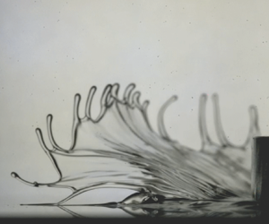
Figure 5. (a) High-speed camera images of the impact of a disk on the highly viscoelastic fluid PEO 4M 10 g l$^{-1}$. Visible is the elastic response of the liquid. After 4 ms the liquid has a tendency to retract itself back into the contact, as a result of the rapid stretching of the polymer molecules during the first moments of impact. In order to be able to create these images, a slightly different set-up was used. This set-up consisted of a disk with flat bottom, size $r_m=2$ cm and mass 550 g. It was dropped with velocity 0.4 m s$^{-1}$ onto a fluid layer of thickness 2 mm. (b) The development of central layer thickness during the impact on four different concentrations of PEO 4M. Impact velocity is 1.3 m s$^{-1}$ for all four measurements. As a result of the elasticity, fluid sucks itself back into the gap after impact, pushing the piston back up, resulting in the typical bump in these curves. The inset shows a zoomed-in version of the region in the dotted rectangular box. The dots are data points measured by the induction sensors, which are connected by a dashed line for visual guidance. As shown in the inset, the elastic end time and the elastic end layer are defined as respectively the time and layer thickness at the peak of the bump. (c,d) The elastic end time $t_e$ (c) and the elastic end layer $h_e$ (d) as a function of impact velocity of the piston and polymer concentration. Both $t_e$ and $h_e$ do not depend on impact velocity, which means that a viscoelastic liquid cannot be squeezed out on a short time scale, explaining the slippery properties of these liquids.

This explanation is further strengthened by the high-speed imaging of the squeezing of a viscoelastic liquid (see figure 5a). For this measurement an additional similar set-up was used to allow for camera capture, as explained in the caption of figure 5. Observed is the initial squeeze out and the elastic recoil occurring within a few milliseconds after impact. The sheet of fluid coming out from underneath the surfaces does not break apart as a Newtonian liquid would do (Sijs & Bonn Reference Sijs and Bonn2020) but contracts itself partly back towards the gap underneath the piston. The characteristics of the elastic recoil are examined further for several concentrations of PEO 4M and over a range of impact velocities. We define the elastic end time $t_e$ and elastic end layer $h_e$ as respectively the time after impact and the central layer thickness for which the layer thickness is at its maximum, as illustrated in the inset of figure 5(b). At this instance the initial elastic impact can be considered finished and the slow viscous regime begins with layer thickness $h_{start}=h_{e}$.

The elastic end layer depends heavily on the concentration (see figure 5d), which is explained by the large difference in viscosity in the liquids. The impact velocity, however, has little effect on the value of $h_e$, meaning that one cannot squeeze out a viscoelastic liquid rapidly by increasing this parameter. The elastic end time depends not on impact velocity and only marginally on concentration (see figure 5c). This result is sensible, as the time scale in which the stretching and relaxing takes place is an intrinsic property of the molecule, independent of the precise amount of those molecules in the solution or the amount of stretching. The elastic end time for the highest (10.0 g l$^{-1}$) and lowest (2.5 g l$^{-1}$) concentrations is slightly lower than for the two intermediate concentrations, yet it is unclear whether there is a physical or experimental reason behind this.

From the rheological parameters it is possible to extract a time scale by dividing the first-normal-stress coefficient by viscosity (Bird et al. Reference Bird, Armstrong and Hassager1987). The precise result of this calculation not only depends on concentration, but is also very sensitive to the way the rheology measurement is performed (de Cagni et al. Reference de Cagni, Fazilati, Habibi, Denn and Bonn2019). From our numerical simulation and from the values obtained by dividing impact velocity by initial layer thickness we find a typical shear rate range between $100$ and $1000$ s$^{-1}$ for the impacts on the viscoelastic liquids. Within this range time scales of between 10 and 50 ms are found for the PEO 4M concentrations (see figure 6a). This time scale has the same order of magnitude as the elastic end time, so likely these quantities are closely linked to each other. This idea is supported by the results for the two mostly inelastic fluids PEO 2M and Xanthan Gum, which have a time scale roughly an order of magnitude lower at the higher end of the shear rate range. This explains why these fluids do not show any viscoelastic behaviour during impact, whilst they do exhibit (small) normal stresses in the rheology measurements. In fact, the concentration of PEO 2M 10.0 g l$^{-1}$ actually yields a higher normal stress than the PEO 4M 2.5 g l$^{-1}$, see figure 1(f,g), but because the former has smaller molecules its relaxation time is much shorter no characteristic bump is found in the impact experiment.

Figure 6. (a) The time scale that can be derived from rheological data by dividing the first-normal-stress coefficient by the viscosity for all six shear-thinning fluids. (b) Development of the central layer thickness as a function of time for three concentrations of PEO 4M impacted by the piston with velocity 1.33 m s$^{-1}$ (data points). The lines display the fits using the Jeffreys model. As the Jeffreys model does not describe shear thinning, it makes no sense to use it for the slow viscous regime, so the curves terminate after a time $2t_e$. (c) The development of the central layer thickness for PEO 7.5 g l$^{-1}$ with four different impact velocities. (d–f) Respectively the values of $\eta _0$, $\lambda _1$ and the ratio $\lambda _2/\lambda _1$ that are found by the fitting process as a function of impact velocity. The dashed line in (d) displays the slightly upwards trends in the viscosity results. For the three highest concentrations of PEO (4M), the ratio in (f) grows towards 1 when lowering the impact velocity, indicating that viscoelastic effects are less prominent at low piston speed. The fitting results for the retardation time $\lambda_2$ can be found in figure 8 in Appendix D.

As a result of $t_e$ and $h_e$ both being constant with respect to impact velocity within the range of parameters tested here, it can be concluded that, for every piston impact, the slow viscous regime starts at the same layer thickness at the same time after impact. It is therefore impossible to completely drain a viscoelastic liquid on a short time scale $\bar {t}$. This explains the slipperiness of the PEO 4M solutions discussed in the introduction, since the gap between foot and surface is lubricated for a relatively long time during the slow viscous regime, giving e.g. the foot or shoe no grip on the surface, resulting in the victim falling. In contrast to stepping on a non-viscoelastic liquid, the kinetic energy the victim provides during his step plays no role, as it will counterintuitively not change the amount of fluid left underneath his foot, as showed by the experiments.

The impact on a viscoelastic fluid can be modelled by a Jeffreys model, which is an often used constitutive equation that adds elasticity to a Newtonian liquid (Bird et al. Reference Bird, Armstrong and Hassager1987)

(8.1)\begin{equation} {\pmb{\tau}} + \lambda_1 \frac{\partial {\pmb{\tau}}}{\partial t} ={-}\eta_0 \left(\dot{{\pmb{\gamma}}} + \lambda_2 \frac{\partial \dot{{\pmb{\gamma}}}}{\partial t} \right). \end{equation}

Here, the shear stress $\pmb {\tau }$ does not solely depend on the present shear rate $\dot {\pmb {\gamma }}$, but also on its past development, as may be apparent by the time dependency in (8.1). The model included three parameters: the Newtonian viscosity $\eta _0$, the relaxation time of the polymer $\lambda _1$ and the retardation time of the polymer $\lambda _2$. Many of those types of fluid models exist, and any choice has advantages and disadvantages. We have chosen the Jeffreys model for its relative simplicity, yet still being capable of reproducing the experimentally observed effects. An obvious disadvantage of this model is its Newtonian behaviour in the absence of any elastic effects, whereas the liquids tested all exhibit clear shear-thinning properties.

In Appendix D it is worked out that a workable formula for the viscoelastic force the fluid applies on the piston is given by the well-known Newtonian viscous force (Maude Reference Maude1961) compensated by a memory function that contains information about the fluid movement in the past

(8.2)\begin{equation} F_{ve}=\frac{-6{\rm \pi} \eta_{0} R^2 \dot{h}(t)}{h_0(t)} \frac{{s_m}^4}{{(1+{s_m}^2)}^2} M(t,t'),\end{equation}

with the memory function $M(t,t')$ defined in the following way:

(8.3)\begin{equation} M(t,t')= \left(1-\frac{\lambda_2}{\lambda_1} \right) \frac{{h_0(t)}^2}{\lambda_1 \dot{h}(t)} \int_{t'={-}\infty}^{t'=t} \frac{\dot{h}(t')}{{h_0(t')}^2} \, {\rm e}^{-({t-t'})/{\lambda_1}} \, {\rm d} t' + \frac{\lambda_2}{\lambda_1}. \end{equation}

The derivation of these formulas relies on an assumption that has not been fully proven mathematically, but we will show here that (8.2) works well as a model to capture the underlying physics for an impact on a viscoelastic fluid. For as long as layer thickness changes significantly within a time scale $\lambda _1$, elastic effects have influence, and otherwise the memory function becomes equal to 1 and the result for ordinary Newtonian squeeze flow remains in (8.2).

The development of the central layer thickness as a result of the viscoelastic force is simulated for modelling the first milliseconds after impact by applying a forward Euler algorithm on the equation of motion given by (3.4). The experimental values $h_{0}(t=0)=X_{0}$ and $\dot {h}(t=0)=-v_{0}$ are used as the initial condition for the simulation and the three parameters $\eta _0$, $\lambda _1$ and $\lambda _2$ are considered fitting parameters that are optimized to match model and data. The $\dot {h}^2$ term of the inertia according to (3.3) was included, but the ‘virtual mass’ term was excluded, since we argue it is unphysical.

The usage of the viscoelastic force given by (8.2) yields a bump in the layer thickness profile that is similarly shaped to the experimental results. The fitting of the parameters $\eta _0, \lambda _1$ and $\lambda _2$ on the experimental data was performed by minimizing the difference between experimental data and simulation for these three characteristics: the lowest point in the bump, the highest point in the bump and the time difference between these points. We do not constrain ourselves in allowing only one set of parameters $(\eta _0,\lambda _1,\lambda _2)$ per fluid, but rather we fit the parameters for each individual impact measurement and interpret the obtained parameters. The viscoelastic effects of the fluid are expected to play no role anymore during the slow viscous regime (Binding et al. Reference Binding, Davies and Walters1976; Engmann et al. Reference Engmann, Servais and Burbidge2005), so for $t > 2t_{e}$ the simulation ends. The precise moment at which to stop the simulation is somewhat arbitrary, yet it has to be done somewhere, as the Jeffreys model is incapable of capturing the shear-thinning behaviour of the slow viscous decay. The simulation can reproduce the impact on the different concentrations of PEO (4M) for different impact velocities (see figure 6b,c).

Just like the viscosity found by the rheometer, the fitted viscosity grows on increasing the polymer concentration, see figure 6(d); the scaling is similar. The impact velocity has little influence on the fitted viscosity, which is remarkable as it could be expected that the shear-thinning properties would cause the fluid to be thinner at higher impact. The results suggest that during the short time scale in which elastic stresses dominate the shear thinning becomes irrelevant. The results for the lower polymer concentrations, 2.5 g l$^{-1}$ and 5.0 g l$^{-1}$, even seem to suggest that the liquid gets thicker for higher impact velocity. However, that the viscoelastic properties during impact are comparable to a shear-thickening effect is something that has been found before (de Goede et al. Reference de Goede, de Bruin and Bonn2019).

The fitted values for the relaxation time $\lambda _1$ fall within a range between 20 and 60 ms, similar to the elastic end time, see figure 6(e). This time scale is thus also in the same range as the elastic end time $t_e$ and the viscoelastic time scale inferred from the rheological data. Therefore, the rheology data might intrinsically contain an estimate for which relaxation time to use in the Jeffreys model. However, the dependence of these parameters on velocity is different for all three: the fitted relaxation time increases with velocity, the elastic end time is constant and the time scale extracted from the rheological data decreases with velocity.

The ratio between retardation time and relaxation time is expected to be between 0 and 1, with 0 resulting in the simpler Maxwell model and with 1 resulting in the complete absence of viscoelastic stresses (Bird et al. Reference Bird, Armstrong and Hassager1987). Simulations with the Maxwell model have been tried and they cause the model to behave too elastic, as the predicted oscillation of the piston continues for too long, so that more than one bump is predicted. The inclusion of the retardation time dampens these oscillations. At an impact velocity above 0.8 m s$^{-1}$ the ratio is found to be $0.25 \pm 0.10$, see figure 6(f). At low impact velocity it is expected that viscoelasticity plays a lesser role, due to the lesser amount of stress imposed on the liquid. This is observed in the trend for the ratio $\lambda _2/\lambda _1$. It grows closer towards 1 when lowering impact velocity, which we interpret as the viscoelastic effects becoming less prominent for these types of impact. (In this limit the Jeffreys model would turn into the simple case of a Newtonian fluid.) It remains unclear to the authors why the concentration 2.5 g l$^{-1}$ displays the opposite trend, although it is noted that a relatively low layer thickness, in some cases close to zero, for this fluid leads to quite extreme simulation conditions, and the convergence of the fit is poorer than for the other concentrations.

With these results, it might be possible to suggest a way to roughly predict the squeeze flow of a viscoelastic liquid from only its rheological data. Firstly, an average shear rate during the squeezing has to be estimated. Then, a characteristic time scale $\lambda _1$ for the viscoelastic regime can be extracted from the ratio between the first-normal-stress coefficient and viscosity at that given shear rate. This time scale serves as the relaxation time in the Jeffreys model. To complete the model, the viscosity $\eta _0$ can be taken from the flow curve at the average shear rate and the retardation time $\lambda _2$ can be assumed to be roughly a factor 4 smaller than $\lambda _1$. Then, (8.2) is capable of predicting the viscoelastic regime of the impact during the time scale $2\lambda _1$, after which slow viscous shear-thinning squeeze described by (3.1) follows until all the fluid is squeezed out of the gap. Although this method is very crude and more experimental evidence is required to verify its correctness, it seems plausible that the relatively simple rheometer measurement contains all information necessary to precisely predict the more complicated fluid behaviour under high velocity impact.