Introduction

Mass losses from glaciers and ice caps outside Antarctica and Greenland are estimated to have accounted for 0.50±0.18mma ⁻ 1 of the observed rate of global sea-level rise from 1961 to 2003 or 0.77±0.22mma ⁻ 1 for the period 1993–2003 alone (Reference SolomonSolomon and others, 2007). The large uncertainty associated with these estimates calls for more accurate and spatially distributed measurements of glacier mass balance.

In order to cover the entire polar regions, surface mass-balance (SMB) observations are carried out from space (Reference ZwallyZwally and others, 2005; Reference Shepherd and WinghamShepherd and Wingham, 2007). One standard method to determine mass changes is provided by satellite radar altimetry. Surface elevation measurements are taken over several time intervals to yield volume changes (Reference WinghamWingham and others, 2001). However, this technique is sensitive to ice topography and radar returns from beneath the surface (Reference Scott, Nienow, Parry, Mair, Morris and WinghamScott and others, 2006) and relies on ground-truth data. Volume backscatter that originates from inhomogeneities within the snow and firn leads to ambiguities in the detection of the surface reflection. Furthermore, knowledge of variations in snow and firn density is critical for accurate conversion of volume changes to mass changes. Both factors need particular consideration in areas where meltwater retention by refreezing is significant and highly variable in space and time.

The SMB of a glacier is reflected in the spatial distribution of its glacier facies. Following the usual textbook definition by Reference PatersonPaterson (1994), areas exclusive of snowmelt are referred to as dry snow facies, generally restricted to the interior of Greenland and Antarctica. The upper accumulation area of Arctic ice caps typically consists of the percolation facies. Here, surface melt occurs during the summer period and meltwater produced at the surface (or rain) infiltrates into the snow, where it refreezes. If, by the end of the summer, the entire snowpack reaches pressure-melting point, the area is referred to as wet snow facies. Here, meltwater might percolate below the last summer surface (LSS) into older layers of firn. The combined area of wet snow, percolation and, where applicable, dry snow facies is often referred to as firn area. Below the lower boundary of the firn area lies the superimposed ice (SI) facies, i.e. ice formed at the base of the snowpack on top of impermeable cold ice, whereas ice layers, lenses and glands within the snow and firn are termed internal accumulation (Reference Hagen, Reeh, Bamber and PayneHagen and Reeh, 2004).

For many Arctic glaciers, accumulation by internal refreezing and SI formation may be spatially and temporally highly variable, but generally represents a significant contribution to the SMB (Reference Woodward, Sharp and ArendtWoodward and others, 1997; Reference Hagen, Melvold, Pinglot and DowdeswellHagen and others, 2003). This variability is expressed by changes of the glacier-facies distribution, and emphasizes the importance of ground-truth data for analysis of space-borne data, especially if collected over Arctic glaciers and ice caps. As glacier facies arise from metamorphism and ablation of the winter snow, they relate to both winter and summer conditions.

Field studies of SMB often involve ground-penetrating radar (GPR) surveys at antennae frequencies of ∼400–1500MHz (P- and L-band) with the primary goal of mapping the distribution of snow (Reference Kohler, Moore, Kennett, Engeset and ElvehøyKohler and others, 1997; Reference TaurisanoTaurisano and others, 2007). The density contrast at the LSS causes an internal reflection horizon (IRH) that can be tracked along continuous profiles. Given adequate post-processing of the data, GPR also enables detailed studies of the near-surface firn stratigraphy (e.g. Reference Dunse, Eisen, Helm, Rack, Steinhage and ParryDunse and others, 2008) and provides a non-destructive method of mapping glacier facies (Reference Wadham, Kohler, Hubbard, Nuttall and RippinWadham and others, 2006; Reference Brandt, Kohler and LüthjeBrandt and others, 2008). This technique has been used for validation of glacier facies inferred from synthetic aperture radar (SAR) data (Langley, 2007; Langley and others, 2007), but has not yet been directly applied as a tool of glacier monitoring.

In this study we present GPR data collected at 800 MHz along some 250 km of profiles across the Austfonna ice cap, Svalbard. We re-analyse GPR data from spring 2004 and 2005, published by Reference TaurisanoTaurisano and others (2007), and extend their time series by including measurements from spring 2006 and 2007. For each year, the thickness of the winter snow is mapped and the glacier facies beneath the winter snow are identified. In doing so, we produce a multi-year sequence of glacier-facies distribution.

Study Site

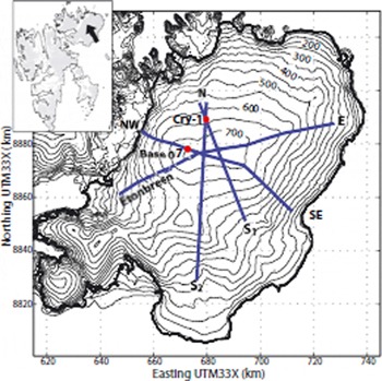
Austfonna is a polythermal ice cap, situated on Nordaustlandet, Svalbard. Centered at 79.7 ^˚ N, 24.0 ^˚ E, it covers an area of 8120 km ^₂ (Fig. 1). The ice cap has a simple dome-shaped topography with well-defined drainage basins, several of which exhibit surge-type behaviour (Reference Hagen, Liestøl, Roland and JørgensenHagen and others, 1993; Reference Dowdeswell, Unwin, Nuttall and WinghamDowdeswell and others, 1999). The maximum elevation of about 800ma.s.l. in the central part coincides with the maximum ice thickness of about 580m (Reference DowdeswellDowdeswell, 1986). Twenty-eight per cent of Austfonna’s bed lies below sea level and it is calving into the Barents Sea along a large portion of its boundary.

Fig. 1.

Map of the Austfonna ice cap on Nordaustlandet. The blue lines indicate the GPR transects measured in 2007, while the red markers show the location of the base camp in 2007 and of study site Cry-1. The inset shows the location of Nordaustlandet within the Svalbard archipelago.

A number of investigations have been made during previous years with the focus on elevation changes and mass balance. Reference Pinglot, Hagen, Melvold, Eiken and VincentPinglot and others (2001) inferred the annual mean SMB of the accumulation area of Austfonna for the period 1986 to 1998/99 from shallow ice cores dated by the detected radioactive fallout horizon from the Chernobyl accident. Maximum values of around ∼0.5mw.e. a ⁻ 1 were measured in the summit area. Reference TaurisanoTaurisano and others (2007) mapped the winter snow cover using GPR data collected in spring 1999, 2004 and 2005. Like Reference Pinglot, Hagen, Melvold, Eiken and VincentPinglot and others (2001), they found an asymmetry in SMB in accordance with the distribution of snow, with twice as much accumulation in the southeast as in the northwest. Both studies conclude that this pattern results from the proximity of the Barents Sea in the east-southeast, providing a significant moisture source for precipitation. Reference TaurisanoTaurisano and others (2007) related snow thickness to all three spatial coordinates by multiple regression to derive an accumulation index for further use in a SMB model by Reference Schuler, Loe, Taurisano, Eiken, Hagen and KohlerSchuler and others (2007). The distribution of snow across Austfonna is therefore relatively well understood, whereas the fate of the snow throughout the summer melt season is only known at a few points from shallow cores and mass-balance stakes. Therefore, large uncertainties remain concerning the spatial and temporal variability of the firn area extent as well as the formation of SI and, hence, estimates of the equilibrium-line altitude (ELA).

Using airborne laser altimetry conducted in 1996 and 2002, Reference Bamber, Krabill, Raper and DowdeswellBamber and others (2004) showed that Austfonna is thinning at lower elevations and thickening in the interior, and explained this by an increase in accumulation. Reference Hagen, Eiken, Kohler and MelvoldHagen and others (2005) pointed out that elevation changes may be driven by both surface processes (accumulation and ablation) and ice dynamics (possible build-up towards surge activity). Reference Bevan, Luckman, Murray, Sykes and KohlerBevan and others (2007) suggested that slow ice dynamics is the key factor for the positive mass balance of the accumulation area, since the actual volume flux across the equilibrium line is only half of the balance flux.

Data Acquisition And Processing

Annual field studies were conducted in spring during 2004– 07, with data collection over 2week periods in late April and early May. GPR and global positioning system (GPS) data were collected along four major transects that cross the ice cap at different orientations, with a total length of about 250 km (Fig. 1). The start and end positions along the transects differ between years by up to 5 km, while the lateral offset is generally smaller than 10m. Due to logistical and technical problems, no GPR data were collected south and southeast of the summit in 2005 and some data gaps occurred in 2006. GPR and GPS surveys were complemented by snow-pit investigations (usually two to four pits for each transect in a particular year) and manual snow-depth sounding (every ∼2 km) using ordinary avalanche probes. Snow pits were excavated down to the LSS. In the ablation and SI area, the LSS was recognized as the snow–ice interface, while in the firn area the LSS appears as either a distinct ice layer or a transition towards large refrozen ice crystals (>3 mm). At some locations in the firn area, the snow pits were extended by 0.5m below the LSS. The bulk density was measured at 20 cm intervals, and snow stratigraphy, temperature, crystal size and hardness were logged.

Ground-penetrating radar and GPS

The GPR data were collected using a commercial impulse-radar system (RAMAC, Malå GeoScience) with shielded antennae at a frequency of 800MHz. A GPS (global navigation satellite system, GNSS) receiver was operated together with the GPR for simultaneous kinematic positioning. The GPR control unit and the GPS system were mounted on one sledge, the GPR antennae on a separate unit made of fibreglass, and pulled by a snowmobile. A driving speed of around 5ms ⁻ 1 and a constant triggering rate of the GPR resulted in a trace interval of 0.25–0.30m. The receiving time window was set to 145 ns in 2007 and 126 ns in previous years, in order to image a depth range of at least 10m. Every trace consists of 1024 samples corresponding to sample intervals of 0.14 ns and 0.12 ns, respectively. GPS measurements were logged at a rate of 1 Hz and post-processed using a stationary GPS as reference. The accuracy of the post-processed GPS data is estimated to be typically better than 10 cm in all three spatial coordinates. Positions of individual traces were allocated by linear interpolation between the post-processed GPS coordinates.

Post-processing of the GPR data included static correction and frequency filtering. Constant time-delay clutter and system artefacts were eliminated using a horizontal filter. For visualization and interpretation of the data, a gain function (energy decay) was applied.

During data acquisition in spring, the snow was entirely at sub-freezing temperatures. The effects of liquid water on the propagation of the radar signal are therefore neglected. The wave speed v of the radar signal in dry snow was derived from the permittivity ε^´ r,

where c is the speed of light in vacuum. We used the empirical relation of Reference Kovacs, Gow and MoreyKovacs and others (1995) to relate snow density (kgm ⁻ 3) to permittivity:

We derive the snow thickness using the two-way travel time (TWT) of the reflection occurring at the LSS and the wave speed. In situ information on snow depth from manual soundings and snow pits ensures that the correct IRH is associated with the LSS.

The error in the depth determination of the LSS mainly arises from lateral variability of the bulk-snow density, and hence wave speed, from the applied constant velocity. In 2007, bulk densities from measurements at 14 snow pits yielded a mean value and related standard deviation of 390±21 kgm ^{− 3}. Applying the above equations yields a wave speed of 2.25±0.03mμs ⁻ 1. Values for the other years were determined following the same procedure.

The GPR system is designed such that the centre frequency corresponds approximately to the bandwidth. The wavelength λ in firn (ρ = 600 kgm ^{− 3}) is ∼0.25 m. The theoretical resolution of λ/4 is therefore about 0.06 m. However, this is limited by the length of the transmitted wavelets, comprising two cycles (approximately 2.5 ns), as interference of partial reflections from inhomogeneities within the length of the wavelets occurs. The effective interface resolution hence equals the wavelength, which for our domain varies from 0.21 m for glacier ice (ρ = 900 kgm ^{− 3}) to 0.29 m for wind-packed snow (ρ = 370 kgm ^{− 3}).

Mapping of Glacier Facies

Glacier facies relate to the surface properties of a glacier and are an expression of its SMB. Reference Wadham, Kohler, Hubbard, Nuttall and RippinWadham and others (2006), Reference LangleyLangley (2007) and Reference Brandt, Kohler and LüthjeBrandt and others (2008) showed the potential of the GPR to map various glacier facies.

The accumulation area is characterized by either firn or SI. On Austfonna, the firn facies consists of wet snow. In certain years, some snow in the summit area might remain at sub-freezing temperatures throughout the entire summer, and a percolation facies may form. The ablation area is typically composed of pure glacier ice. Firn, SI and glacier ice are recognized by their characteristic signal reflection pattern (Fig. 2) dependent on typical occurrence and strength of dielectric contrasts (Reference Brandt, Kohler and LüthjeBrandt and others, 2008). Due to its homogeneous properties, pure, cold glacier ice is predominantly transparent to electromagnetic waves and signal reflections barely occur. In the firn area, the strong dielectric contrast between solid ice clusters and an often coarse-grained firn matrix causes IRHs of strong amplitudes, while a varying air-bubble content in the SI causes IRHs of lower amplitude.

Fig. 2.

GPR classification of glacier facies along a 30 km long transect from the summit area (F1) into the ablation area (GI) of Etonbreen. The green line indicates the position of the LSS. The lower panels show close-ups of 2 km GPR data with characteristic signal reflection patterns.

We use these properties to map the facies underneath the winter snowpack: firn (F), SI and glacier ice of the ablation area (GI) (Fig. 2).We further sub-categorize the classification F into a long-term firn area (F1); a firn layer that originates from multiple years of accumulation, but lies in a zone of recent (∼10 years) variability of the firn line (F2); and a thin firn layer that apparently originates from one accumulation season only (F3). Regions where strong IRHs indicate firn over most of the depth range of the GPR image (6m and more, corresponding to ∼10 or more mass-balance years) are classified as the long-term firn area. IRHs in F2 typically show a larger spatial variability than in F1 and typically converge with the LSS at lower elevations. IRHs in the SI area generally show an even larger spatial variability. The formation of SI requires ponding of free water and is therefore strongly controlled by local topography (Reference Brandt, Kohler and LüthjeBrandt and others, 2008). According to the above definition, direct transition from F2 to SI is possible. Transition from SI to F2, on the other hand, involves at least two consecutive years of firn accumulation at a particular location. SI has to be initially covered with a thin layer of firn in one year (F3) to reach the F2 classification in the subsequent year.

In the following, the term glacier facies always relates to the glacier facies beneath the winter snowpack. GPR measurements in spring (year n) therefore yield the thickness of the winter snow accumulation (year n) and the extent of the glacier facies at the end of the previous summer (year n − 1). Measurements of snow accumulation are related to the winter balance only. Glacier facies result from a combination of snow accumulation and subsequent metamorphism and ablation of the winter snow cover. Therefore, the above method of detecting glacier facies also provides a measure of summer conditions. In re-analysing the GPR data from 2004 to 2007, we derive a multi-year sequence of glacier-facies distribution along the transects that allows us to study their interannual fluctuations. It should be noted that the classification of GPR data is a somewhat subjective process. However, the same processing has been applied to the entire dataset and the classification was performed by a single person to ensure consistent interpretation.

Validation

To gain more confidence in our interpretation of the GPR data, we first compare the GPR images with the vertical density profiles from neutron probing, and find a clear relation between the observed density profiles and the signal reflection pattern in the radar image. We then compare the GPR-derived glacier facies with radar zones in the SAR image of Austfonna.

Neutron-scattering probe

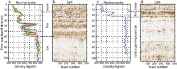
The six density profiles recovered at the base camp are shown in Figure 3a. The site lies in an area classified as F1, the long-term firn area. The winter snowpack is characterized by densities between 350 and 450 kgm ^{− 3}, in agreement with measurements in a nearby snow pit. The LSS is recognizable as a sharp density increase at approximately 14 ns TWT, corresponding to a depth of 1.7 m. The digitized LSS from GPR is at the same depth (Fig. 3b). From the LSS down to 33 ns the densities are in the range 470–570 kgm ^{− 3}, which is typical for firn. Values in the range 550–850 kgm ^{− 3} occur between 33 and 60 ns and indicate firn and ice layers. In the GPR image, this depth range is characterized by strong reflection amplitudes, without resolving individual IRHs. At around 60 ns (∼6m depth), the firn–ice transition is reached. Below this depth range, the density varies around 860 kgm ^{− 3} and the signal reflections in the GPR image are much weaker.

Fig. 3.

Comparison of vertical density profiles, inferred from neutron-scattering probing with GPR signal reflections obtained along ∼120m sections at (a, b) base camp and (c, d) Cry-1. The dashed lines in the GPR images indicate the position of the LSS as confirmed from snow pits and manual snow-depth soundings.

The classification at Cry-1, north of the summit, is F3 for summer 2005 and F2 for 2006. The neutron-probe profile reveals densities between 500 and 630 kgm ^{− 3} from the LSS at 13 ns down to 22 ns TWT (Fig. 3c). Below, the density sharply increases to approximately 850 kgm ^{− 3}, indicating the firn–ice transition at a depth of about 2.4 m. In the GPR data, the transition produces an IRH at that depth (Fig. 3d), separating a region of strong reflection amplitudes above (firn) from lower reflection amplitudes below (ice).

SAR zones

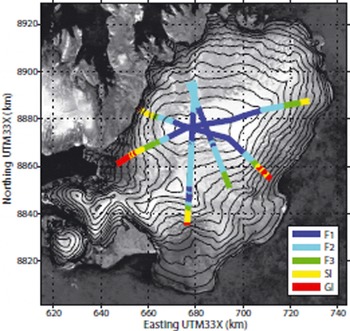
To compare the backscatter zones of the SAR image with the GPR results, we plot the colour-coded glacier facies, inferred from GPR, on top of the 2-D backscatter image (Fig. 4). The backscatter intensities of the SAR signal represent an integral of all backscatter sources from the illuminated volume (Reference König, Wadham, Winther, Kohler and NuttallKönig and others, 2002). While the dry winter snow has only minor effects on the SAR signal, the properties of the firn and ice below the LSS control the penetration depth of the signal. In the firn area, volume scatter from inclusions of solid ice clusters dominates and results in high backscatter intensities (light grey shades/white). In the ablation area, volume backscatter from relatively homogeneous glacier ice is insignificant and a distinct snow–ice interface leads to specular reflection of energy away from the side-looking instrument, resulting in low backscatter intensities (dark grey shades). SI is characterized by a varying air-bubble content that causes medium backscatter intensities.

Fig. 4.

Comparison of GPR-derived glacier facies distribution in summer 2006 with a 2-D backscatter SAR image. The image is an average of a number of winter scenes acquired during 2005–07.

The most striking feature of the comparison is that sections of the GPR transects classified as F1 fall within the limits of the high-backscatter area. Furthermore, the transition between F1 and F2 coincides with the boundary that separates areas of high backscatter from areas of medium backscatter. Sections of the GPR transects classified as GI coincide with areas of low backscatter. The good agreement with the SAR data gives further confidence in the GPR-based glacier-facies classification, as previous studies have shown that SAR and GPR systems yield very similar results (Reference LangleyLangley, 2007; Reference Brandt, Kohler and LüthjeBrandt and others, 2008).

Results

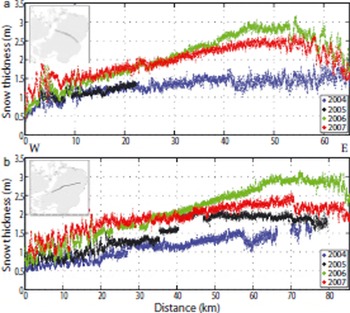
The observed distribution of snow accumulation in 2006 and 2007 reconfirms the asymmetric snow distribution found by Reference Pinglot, Hagen, Melvold, Eiken and VincentPinglot and others (2001) and Reference TaurisanoTaurisano and others (2007). Figure 5 shows two transects running from the western to the eastern margin. In the 4 year period 2004–07, the snow thickness typically varied from 0.5 to 1.5m in the west, and from 1.5 to 3m in the east. The lowest snow accumulation was measured in spring 2004, with a mean thickness of 1.21m over the entire length of the two transects. In spring 2006, a mean thickness of 2.01m was measured over the same distance.

Fig. 5.

Snow thickness profiles for spring during 2004–07: (a) along the northwest–southeast and (b) southwest–east transect.

Glacier facies and their temporal variation

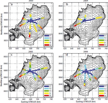
collected in spring during 2004–07, the GPR data yield the extent of the glacier facies at the end of the summer from 2003 to 2006. We investigate fluctuations during this period by plotting the colour-coded facies on top of a contour map of Austfonna (Fig. 6). The most striking feature is a significant increase in the extent of the firn area, beginning in winter 2004/05. In 2003 and 2004, the firn facies was confined to the summit area and SI was exposed along large portions of the transects (Fig. 6a and b). In the subsequent two years, SI became to a large extent covered by firn (Fig. 6c and d). We further note firn pockets (F2) within the upper parts of the SI in 2003, which were no longer present in 2004. The lower boundary and the total change of the firn area, both in vertical and lateral dimensions, are listed for each profile in Table 1. No differentiation has been made as to whether the firn originates from the previous year or not. In addition, estimates of the ELA inferred from the mass-balance stakes on Etonbreen are provided. Between 2003 and 2006, the firn line decreased by ∼40–100m elevation in the north and west of Austfonna and 150–230m in the south and east. This corresponds to a lateral expansion of the firn area by up to 7.3 km along profiles in the north and west and up to 13.3 km for the southern and eastern profiles.

Fig. 6.

Colour-coded glacier facies at the end of the summer from 2003 to 2006 along the GPR transects in spring during 2004–07, plotted on top of a contour map of Austfonna with 50m contour interval.

Table 1.

Approximate firn-line elevations along the GPR profiles from the end of the summer 2003 to 2006, total change during that period and corresponding lateral expansion (estimates of the ELA from mass-balance stakes on Etonbreen are also given)

To visualize the interannual changes in more detail, and to allow direct comparison between measurements from different years, we select a transect along which data were collected in all years. We plot the extent of the glacier facies along the profile that runs from Etonbreen in the west via the summit towards the east (Fig. 7). The increase of the area classified as F2 or F3 in the period summer 2004 to summer 2006 is clearly seen. For each year, a progressively larger portion of the sections classified as SI is covered by an expanding and thickening layer of firn. However, the sections with deep firn F1 show little interannual variation. This highlights the fact that F1 originates as an integral of many years of firn accumulation. The only notable change in the extent of F1 occurs between 2005 and 2006, when it advances slightly. The minimum extent of the total firn area (F1, F2 and F3) in the period summer 2003 to summer 2006 is reached in summer 2004. A large portion of SI is exposed along the transect. In 2003, several firn pockets (F2) between 1 and 3 m thick and with cross-sectional lengths of tens to hundreds of metres (likely originating from multiple years of firn accumulation) overlie the SI (15–20 km). In 2004, no such pockets were identified, indicating that they have been melted away or transformed into SI. Figure 7 also indicates estimates of the ELA, inferred from mass-balance stakes on Etonbreen in the western part of the transect. The ELA decreased from 650 m in 2004 to 500 m in 2004 and 470 m in 2006. These elevations fall within the zone classified as SI in the corresponding year.

Fig. 7.

Colour-coded glacier facies along the transect from Etonbreen in the west via the summit area towards the east. Each stripe represents the classification for a particular year in chronological order, with 2006 at the top and 2003 at the base. Note that the thickness of the stripes is not related to the actual snow thickness or depth. Black markers indicate ELA estimates inferred from mass-balance stakes on Etonbreeen for the period 2004–06.

We also tracked characteristic IRHs within the firn over time. These represent the summer surfaces from the previous year. This analysis is not as robust as the mapping of glacier facies, but we found that the position of the IRHs in relation to the LSS remains apparently unchanged in the period spring 2004 to spring 2005. In subsequent years, the IRHs are progressively buried at a rate of the order 1ma ⁻ 1.

Concluding Remarks

Comparing the sequence of glacier-facies distribution with direct SMB measurements, we have to bear in mind some limitations on the information content of the mapped facies. Theoretically, the ELA corresponds to the lower boundary of the SI in a particular year. The fact that the ELAs from the mass-balance stakes lie above the GPR-derived transition from SI to GI (Fig. 7) illustrates the limited ability of the GPR data to pinpoint the exact position of the ELA. Although SI can be identified from theGPR data, it remains undetermined whether this is old SI and subject to ablation or newly formed SI that contributes positively to the SMB. A similar limitation applies to detection of the recent firn line (the snow line by the end of the previous summer). In the case of a growing firn area, the firn line coincides with the lower boundary of the firn area. In the case of a shrinking firn area, as in summer 2004, the recent firn line might retreat to a position within the multi-year firn (F1 and F2) and its determination may be ambiguous. Although the position of the ELA cannot be directly inferred from an individual facies distribution, its interannual variation is captured in the multi-year sequence.

The observed increase in the extent of the firn area, beginning in summer 2004, is in line with a lowering ELA as derived from the mass-balance stakes on Etonbreen over the same time period (Table 1). Between summer 2003 and summer 2006, the firn line lowered by ∼40–100m elevation in the north and west and 150–230m in the south and east of the ice cap, corresponding to a lateral expansion of the firn area along the profiles by up to 7.3 and 13.3 km, respectively. The apparently constant position of characteristic IRHs in spring 2004 and spring 2005 indicates that the entire winter snow has been heavily affected by summer melt, such that it is not recognizable in the GPR data. The concurrent disappearance of several firn pockets within the SI area provides further evidence of strong surface melt in summer 2004. This does not necessarily represent a complete absence of net accumulation, since it is likely that meltwater was retained through internal accumulation and SI formation.

This study demonstrates GPR as a non-destructive and useful tool to map glacier facies. As well as measuring the amount of winter snow, we obtained a multi-year sequence of glacier-facies distribution. This can be interpreted in terms of SMB variations. In addition, these facies provide valuable ground-truth data for validation and interpretation of satellite radar altimetry data, such as from Envisat or the upcoming CryoSat-2.