


1. Introduction
1.1. Physiological background
The aortic valve regulates the oxygenated blood flow from the heart to the rest of the organs. This valve is located between the left ventricle and the aorta, and possesses three flexible cusps. Diseases of the aortic valve make up a significant portion of valvular heart diseases (Iung & Vahanian Reference Iung and Vahanian2011), which mainly involve thickening of the valve cusps (aortic stenosis). In severe conditions, the diseased valve must be replaced by a prosthetic valve (Yoganathan, He & Casey Reference Yoganathan, He and Casey2004; Sotiropoulos, Le & Gilmanov Reference Sotiropoulos, Le and Gilmanov2016).
One example of widely used prosthetic heart valves is the bileaflet mechanical heart valve (BMHV). This consists of two semi-elliptical metallic plates which regulate blood flow by pivoting in a ring-shaped housing frame (see figure 1a). These valves are favoured for younger patients thanks to their high durability. However, BMHVs are associated with high risk of blood clotting, for which the recipients of these valves should receive life-long blood thinning drugs to combat the risk of stroke. Shear-induced platelet activation (Holme et al. Reference Holme, Ørvim, Hamers, Solum, Brosstad, Barstad and Sakariassen1997; Alemu & Bluestein Reference Alemu and Bluestein2007), which is linked to turbulent blood flow in the valve, has been attributed to the platelet activation process. It is therefore beneficial to improve the flow in BMHVs, perhaps through design modifications, to mitigate the risk of blood clotting and stroke. Recent efforts in this area include passive control via deploying vortex generators (Hatoum & Dasi Reference Hatoum and Dasi2019) or superhydrophobic surfaces (Hatoum et al. Reference Hatoum, Vallabhuneni, Kota, Bark, Popat and Dasi2020) on the valve leaflets, both with the goal of reducing the intensity of turbulent flow downstream of the valve.

Figure 1. (a) Leading-edge view of a Regent mechanical valve (https://www.structuralheartsolutions.com). The valve leaflets are hinged within a metal frame housing, which is sutured to the aortic root. (b) Leaflet kinematics of BMHV: (–) numerical fluid–structure interaction simulation of Borazjani et al. (Reference Borazjani, Ge and Sotiropoulos2008) and ( $\circ$) experimental investigation of Dasi et al. (Reference Dasi, Ge, Simon, Sotiropoulos and Yoganathan2007). The shaded area in blue shows the interval in which the valve is fully open, while the shaded area in grey shows the valve opening phase.
1.2. Brief overview of BMHV fluid mechanics
The fluid mechanics of BMHVs have been previously studied using experimental (Ge et al. Reference Ge, Dasi, Sotiropoulos and Yoganathan2008; Bellofiore, Donohue & Quinlan Reference Bellofiore, Donohue and Quinlan2011; Haya & Tavoularis Reference Haya and Tavoularis2016) and computational (Dasi et al. Reference Dasi, Ge, Simon, Sotiropoulos and Yoganathan2007; Borazjani, Ge & Sotiropoulos Reference Borazjani, Ge and Sotiropoulos2008; Yun et al. Reference Yun, McElhinney, Arjunon, Mirabella, Aidun and Yoganathan2014b) investigations. These studies revealed a complex flow scenario including multiple instability mechanisms interacting in a confined and complex geometry. The flow in the wake of the valve is described as chaotic or turbulent, which has been attributed with shear-induced platelet activation risk in the bulk flow as well as in the hinge area of these prostheses (Yun et al. Reference Yun, Wu, Simon, Arjunon, Sotiropoulos, Aidun and Yoganathan2012; Hedayat, Asgharzadeh & Borazjani Reference Hedayat, Asgharzadeh and Borazjani2017; Hedayat & Borazjani Reference Hedayat and Borazjani2019). Hedayat et al. (Reference Hedayat, Asgharzadeh and Borazjani2017) showed that the platelet activation potential was significantly higher for BMHVs than bioprosthetic valves (i.e. valves with soft tissue cusps to mimic the native valve) at peak flow. They speculated that this could be due to the larger extent of small-scale structures for this flow. In addition to platelet activation, the relation of a flow rich in small-scale vortices and red blood damage has been studied by Quinlan & Dooley (Reference Quinlan and Dooley2007). Their results showed that the root mean square of the fluid stress on cells is at least an order of magnitude less than the Reynolds stress, which is in line with the hypothesis that smaller flow eddies cause more stress on the blood cells.
The importance of vortical or turbulent flows to the forces exerted on blood components demands more investigation of the mechanisms of laminar–turbulent transition in flow through BMHVs. This can provide a more in-depth understanding of the turbulent flow and also point towards efficient ways to delay or reduce turbulence in these prostheses. Despite this importance, little attention has been paid to this area, perhaps due to the complexity of the flow. Dasi et al. (Reference Dasi, Ge, Simon, Sotiropoulos and Yoganathan2007) used experimental and numerical tools to study the vorticity dynamics in a BMHV. They discussed the resulting coherent structures such as vortex rings and shear-layer instabilities, but the quantitative underpinnings of disturbance growth mechanisms leading to these vorticity phenomena were not addressed. Bellofiore et al. (Reference Bellofiore, Donohue and Quinlan2011) conducted a more elaborate experimental study using up-scaled model of the valve. Using specific flow probes located downstream of the leaflets, they reported principal frequencies by calculating the frequency spectrum for an impulsively started flow as well as a systolic waveform. Based on their up-scaled model, they reported flow field data at higher spatial and temporal resolutions compared with experiments at physiologic scales. In particular, their results showed vortices entering the wake of the valve from within the leaflets, but the origin of these vortices was not investigated. They reported shedding frequencies as high as 152 Hz ( $St=0.23$, based on the projection of the leaflet length on the cross-stream plane and maximum free-stream velocity). Time history of velocity fluctuations showed that the peak frequency corresponds to peak flow time and locations downstream of the leaflets’ central orifice. Motivated by this outcome and by the existing insight on flow around blunt plates in canonical settings (Hourigan, Thompson & Tan Reference Hourigan, Thompson and Tan2001), Zolfaghari & Obrist (Reference Zolfaghari and Obrist2019) investigated the potential source of the high-velocity disturbances in the wake of the BMHV. Resorting to a bottom-up approach and employing a two-dimensional submodel, they showed that the impinging leading-edge vortex (ILEV) instability has a strong influence on the breakdown to chaotic flow in the wake of the valve.
1.3. ILEV instability in BMHVs
BMHV leaflets are mounted at a low angle of incidence ( $5^\circ$) during a significant part of a typical heartbeat (Borazjani et al. Reference Borazjani, Ge and Sotiropoulos2008). Because the Reynolds number (based on the aortic diameter and the mean inflow velocity at peak flow rate) can reach values as high as $Re=10\,000$, this flow configuration becomes highly susceptible to developing an ILEV instability (Deniz & Staubli Reference Deniz and Staubli1997; Hourigan et al. Reference Hourigan, Thompson and Tan2001) downstream of the leaflets’ leading edges. The ILEV instability has been addressed using several canonical configurations (i.e. usually horizontal blunt plates at different chord-to-thickness aspect ratios and Reynolds numbers). These studies reveal a complex mixture of convective and absolute instabilities (Soria & Wu Reference Soria and Wu1992), which could significantly affect the flow downstream of the trailing edge of these plates (Naudascher & Wang Reference Naudascher and Wang1993). Having noticed these findings, Zolfaghari & Obrist (Reference Zolfaghari and Obrist2019) investigated the local linear instability of the ILEV flow scenario in the BMHV. Using a two-dimensional submodel justified by the shape of the BMHV leaflets, unstable temporal Orr–Sommerfeld modes were obtained for this flow. The cusp map procedure (Kupfer, Bers & Ram Reference Kupfer, Bers and Ram1987) was then applied to the velocity profiles in the ILEV zone, where a pocket of absolute instability was identified. It was shown by means of two-dimensional (2-D) direct numerical simulation (DNS) that the absolute instability (wave maker) could be eliminated using a suitable modification of the leaflet's shape, which subsequently preserved the laminar flow in the wake of the BMHV.
1.4. Scope and structure of the present work
Although the 2-D DNS of Zolfaghari & Obrist (Reference Zolfaghari and Obrist2019) and experimental investigations of Bellofiore et al. (Reference Bellofiore, Donohue and Quinlan2011) both show incoming vortices from the central orifice causing high-frequency flow oscillations and small-scale flow structures, it is useful to reproduce these phenomena using 3-D DNSs. Taking into account the complex 3-D structure of the valve leaflets not only enhances our view regarding turbulent flow in the wake of the valve, but also reveals the structure of primary mechanisms at the leading edges of the leaflets.
From a hydrodynamic stability standpoint, even though the work of Zolfaghari & Obrist (Reference Zolfaghari and Obrist2019) provides insight on local parallel flow instabilities of ILEV structures in BMHV, a 2-D global analysis is needed to further demonstrate the 2-D spatial structure of this instability. The use of global instability analysis (Theofilis Reference Theofilis2011) allows a more targeted geometric design effort for ameliorating turbulent flow in the wake of the BMHV. Finally, both the local parallel and the 2-D global instability analyses only consider the ILEV zone and disregard the effect of other wave makers in the system. It is thus important to re-evaluate the role of the ILEV instability in disturbance energy growth in comparison with other driving mechanisms such as the flow in the cavities. To this end, a gradient-based approach will be chosen as it can quantify whether instability growth in the wake area is more strongly promoted by the ILEV instability mechanism or by alternative and competing mechanisms.
In this present study, we first present a 3-D DNS of systolic BMHV flow. We model the systolic flow within a 3-D model, which involves fully open leaflets following the kinematic assumptions given in Zolfaghari & Obrist (Reference Zolfaghari and Obrist2019) and Bellofiore et al. (Reference Bellofiore, Donohue and Quinlan2011). We make use of our in-house multi-GPU data-parallel incompressible Navier–Stokes solver (Zolfaghari & Obrist Reference Zolfaghari and Obrist2021) for generating the DNS data at very high resolution (a total of 337 644 801 grid points were used). This simulation was completed in 3 days on 20 GPUs of the Cray XC40/50 ( $Piz\ Daint$). An equivalent simulation using our massively parallel CPU-based solver (Henniger, Obrist & Kleiser Reference Henniger, Obrist and Kleiser2010b) would have taken 1.5 years to complete with equivalent compute node resources. To our knowledge, this is by far the highest grid resolution that has been used in a heart-valve simulation. The velocity fields and the Lagrangian coherent structures show the complex nature of ILEV instabilities and demonstrate the role these instabilities play in the onset and intensity of turbulent flow past the valve.
Second, a 2-D global linear instability formulation is developed (Theofilis Reference Theofilis2011) for a subdomain attached to the leading edge of only one leaflet. The considered area was sufficiently large to cover the full extent of the time-averaged ILEV. We calculated the temporally unstable modes of this flow by performing a temporal Fourier decomposition of the linearised Navier–Stokes equations (LNSE). Two zero-frequency unstable global modes were identified. Furthermore, we calculated the adjoint of these global modes to obtain their structural sensitivity to the local momentum feedback sources (Hill Reference Hill1992; Giannetti & Luchini Reference Giannetti and Luchini2007). Regions of high sensitivity were concentrated over the wave-maker zone for one mode (mode A), while high sensitivities were also found upstream of the wave-maker zone for the second mode (mode B). This could be related, although not shown here, to the capability of the wave maker itself to amplify the disturbances (mode A), as well as cooperation of the wave maker and base flow (which includes recirculation over the wave-maker zone) to amplify or weaken the unstable mode (mode B). Using the sensitivity fields, we attempted to stabilise the flow by introducing local momentum feedback sources. To this end, small bluff bodies were introduced at areas of high structural sensitivity, and the effectiveness of these scenarios was tested using 2-D DNS. This approach failed for mode A, as expected, because its region of high sensitivity was relatively far from the wall. As a result, the introduced bluff body created more instability owing to the high Reynolds number of the flow. However, the same approach worked well for mode B, where it resulted in reduced flow oscillations between and downstream of the leaflets.
Third, we examine the effect of ILEV instability on energy growth downstream of the instability source, particularly near the trailing edge and in the wake of the valve. We resort to the 2-D submodel of Zolfaghari & Obrist (Reference Zolfaghari and Obrist2019) and develop a gradient-based procedure to obtain optimal initial conditions for achieving maximum disturbance energy growth for specific locations in the flow. The LNSE are solved over the full domain, so that possible contributions of other instability mechanisms in the system can be accounted for. We define a cost functional to maximise the energy growth within a user-defined geometric mask and to simultaneously constrain the magnitude of the initial energy. After validating the adjoint looping formulation using transient growth calculations for plane channel flow at  $Re=3000$ (Reddy & Henningson Reference Reddy and Henningson1993), we performed iterative direct–adjoint looping simulations using various masks at various times. It was found that for sufficiently large times the optimal initial conditions for maximum disturbance energy growth are focused around the leading edge of the leaflet, including the ILEV zone. This was further confirmed for masks that were located between the leaflets (high probability of ILEV contribution), at the trailing edge of the leaflets, and in the wake of the valve. The latter case required more time to reveal the leading-edge instability signature, which was more apparent closer to the instability source, i.e. between the leaflets.
2. Direct numerical simulation
We model the flow with the non-dimensional Navier–Stokes equations for incompressible flow
 \begin{equation} \frac{\partial{\tilde{\boldsymbol{\mathsf{u}}}}}{\partial{t}}+ \tilde{\boldsymbol{\mathsf{u}}}\boldsymbol{\cdot}{\boldsymbol{\nabla}{\tilde{\boldsymbol{\mathsf{u}}}}} ={-}\boldsymbol{\nabla}{\tilde{p}}+\frac{1}{Re}{\nabla}^2{\tilde{\boldsymbol{\mathsf{u}}}}+ \tilde{\boldsymbol{\mathsf{f}}},\quad \boldsymbol{\nabla}\boldsymbol{\cdot}\tilde{\boldsymbol{\mathsf{u}}} =0, \end{equation}
where  $\tilde {\boldsymbol{\mathsf{u}}}$ denotes the velocity field, $\tilde {p}$ stands for pressure and $\tilde {\boldsymbol{\mathsf{f}}}$ is the body force density (non-dimensional quantities are indicated by $\tilde {\cdot }$). The Reynolds number is defined as
 \begin{equation} Re = \frac{\mathscr{U}_0\mathscr{L}_0}{\nu}, \end{equation}
where  $\mathscr {U}_0=0.75$ m s $^{-1}$ (one half of the inflow velocity at peak flow rate,), $\mathscr {L}_0=3\times r_r=36$ mm (three times the aortic root radius) and $\nu =2.7\times 10^{-6}$ m $^2$ s $^{-1}$ are the velocity scale, length scale and the kinematic viscosity ( $\nu ={\rho }/{\mu }$), respectively.
The equations (2.1a,b) are solved using a sixth-order finite-difference scheme in space on a staggered Cartesian grid, and a third-order explicit low-storage Runge–Kutta scheme in time (Henniger et al. Reference Henniger, Obrist and Kleiser2010b; Zolfaghari et al. Reference Zolfaghari, Becsek, Nestola, Sawyer, Krause and Obrist2019; Zolfaghari & Obrist Reference Zolfaghari and Obrist2021). The solver has been exhaustively validated and used to study various transitional flows (Henniger, Kleiser & Meiburg Reference Henniger, Kleiser and Meiburg2010a; Obrist, Henniger & Kleiser Reference Obrist, Henniger and Kleiser2012; John, Obrist & Kleiser Reference John, Obrist and Kleiser2014, Reference John, Obrist and Kleiser2016). For integrating complex surfaces (e.g. valve leaflets) into the Cartesian grid solver, sharp-interface immersed boundary techniques are used (Mittal & Iaccarino Reference Mittal and Iaccarino2005; Mittal et al. Reference Mittal, Dong, Bozkurttas, Najjar, Vargas and von Loebbecke2008; Zolfaghari, Izbassarov & Muradoglu Reference Zolfaghari, Izbassarov and Muradoglu2017).
2.1. Configuration of the numerical simulation
2.1.1. Kinematic assumptions
The kinematics of the BMHV leaflets (figure 1b) consist of a rapid opening ( ${\rm \Delta} t\approx 20\text {--}50$ ms) at the onset of systole (Vennemann et al. Reference Vennemann, Rösgen, Heinisch and Obrist2018), a longer phase ( ${\rm \Delta} t\approx 350$ ms for a typical heart rate at rest) where the leaflets remain in the open position and a rapid closing ( ${\rm \Delta} t\approx 25$ ms) (Dasi et al. Reference Dasi, Ge, Simon, Sotiropoulos and Yoganathan2007; Borazjani et al. Reference Borazjani, Ge and Sotiropoulos2008; Yun et al. Reference Yun, Dasi, Aidun and Yoganathan2014a). The valve leaflets remain fully open at a low angle of incidence ( $5^\circ$) during a large part of systole, which provides a suitable configuration for the creation of ILEV instabilities, as for larger angles of incidence the flow features will differ markedly from ILEV (Deniz & Staubli Reference Deniz and Staubli1997). Starting from the time instant that the leaflets are fully open, we focus on the systolic acceleration phase, which spans approximately 200 ms. Similar to Bellofiore et al. (Reference Bellofiore, Donohue and Quinlan2011) and following additional justifications presented in Zolfaghari & Obrist (Reference Zolfaghari and Obrist2019), we assume that the leaflets are fixed at an angle of $\theta =5^\circ$.
2.1.2. Three-dimensional aortic root and valve model
We define our 3-D model, as an extension of the 2-D model used in Zolfaghari & Obrist (Reference Zolfaghari and Obrist2019). We place the leaflets of a bileaflet mechanical heart valve in the fully open position (position 1 in black colour in figure 2a). The sinuses of Valsalva are included in the 3-D model as three spherical cavities with a radius of  $r_s$ (figure 2b, bottom). The centres of these cavities are located on the $x=0$ plane and fall on the sides of an equilateral triangle, to which the aortic root's cross-section is circumscribed. Leaflets of the BMHV are modelled as blunt plates with a triangular leading- and trailing-edge geometry (figure 2a). The spanwise view of the leaflets is provided on the top panel of figure 2(b). The model geometry resembles the semi-elliptical trailing edge of a Regent BMHV. The leaflets’ thickness faces at leading and trailing edges follow the same geometry as this prosthesis. The main differences between the 3-D model geometry and a Regent BMHV are the absence of the housing ring and the valve ear/hinge recess in the 3-D model. However, these differences are located far from the centreline, hence they are not expected to notably affect the bulk flow downstream of the central orifice which is of interest in this paper.

Figure 2. (a) A 3-D model of the BHMV in the aortic root. The 2-D cross-sections of leaflets in their plane of symmetry are shown in (1) open and (2) closed positions. (b, bottom) The cross-section of the root model at  $x=0$ is shown. The three grey solid points indicate the centres of the spherical cavities representing the sinuses of the Valsalva. These cavities are positioned on the centres of the sides of an equilateral triangle, to which the aortic root cross-section is circumscribed ( $r_s={r_r\sqrt {3}}/{2}$). (b, top) The geometry of the leaflet in the spanwise direction. The spanwise profile of the leading edge of the leaflet is modelled as a semicircle whose centre is located on the domain's axis of symmetry and on the leading edge (grey cross mark), and has a radius of $l_l$. All geometrical parameters of the model except those related to the cavities are given in table 1.
2.1.3. Boundary conditions and flow forcing
The flow is smoothly accelerated from zero to the mean velocity of  $\mathscr {U}_{in}=2\mathscr {U}_0$ at $t=200\,{\rm ms}$ (figure 3). No-slip boundary conditions are imposed via an immersed boundary method on the rigid valve leaflets and aortic root boundaries. Periodic boundary conditions are specified in the streamwise direction $x$, where the systolic waveform is forced using a fringe region technique (Nordström, Nordin & Henningson Reference Nordström, Nordin and Henningson1999) upstream of the valve
 \begin{equation} \tilde{\boldsymbol{\mathsf{f}}}=\boldsymbol{\lambda(x)}(\tilde{\boldsymbol{\mathsf{u}}}- {\tilde{\boldsymbol{\mathsf{u}}_0}}(t)), \end{equation}
where  $\lambda (x)$ is the fringe function and $\tilde {\boldsymbol {u}}_0(t)$ is a uniform flow profile. The amplitude of $\tilde {\boldsymbol {u}}_0(t)$ and the fringe function $\lambda (x)$ are tuned $\textit {ad~hoc}$ to provide the desired systolic flow acceleration (figure 3). The fringe region forces the appropriate inflow profile, and simultaneously damps out the outflow disturbances re-entering the domain at the domain's inlet due to periodic boundary conditions.
Table 1. Geometrical parameters of the 3-D model.


Figure 3. Acceleration part of the waveform used in the DNS. The horizontal dashed line marks the peak flow rate, corresponding to a mean flow velocity  $\mathscr {U}_{in}=2\mathscr {U}_0$.
A highly resolved numerical simulation using  $2561\times 513\times 257= 337\,644\,801$ degrees of freedom in a cuboid domain of size $3r_r\times 3r_r\times 15r_r$ is performed. Such a high spatial resolution is set to deal with the non-conforming geometry of the leaflets, and also to resolve the spatio-temporal instability waves and their interactions (refer to the effect of grid resolution in Zolfaghari & Obrist Reference Zolfaghari and Obrist2021). Grid stretching is applied in all three directions, so that a grid resolution similar to the one reported by Zolfaghari & Obrist (Reference Zolfaghari and Obrist2019) is achieved near the leaflets (31 grid points are placed along each leaflet's thickness length $\delta _l$). A dimensionless time-step size of $d{t}=10^{-4}$ was set, and a total of 29.1K time steps were integrated (up to the physical time of $t\approx 200\,{\rm ms}$). To the best of our knowledge, this is the highest resolution that has been used for a numerical simulation of BMHV flow using the incompressible Navier–Stokes equations. This simulation was completed using our novel hybrid multi-GPU task and data parallel Navier–Stokes solver on 20 GPUs in three days. Because our GPU-based implementation is approximately 150 times faster than the CPU-based MPI-parallel flow solver (using the same node configuration, i.e. 20 nodes of Cray XC40/50, Piz Daint), the present simulation ported onto an equivalent number of CPU cores ( $20\times 16=320$ cores with hyper-threading) would have taken approximately 1.5 years to complete. The size of each data output of the velocity field amounted to $\approx$8.1 GB. Further details on this DNS and the numerical and parallelisation methodologies can be found in Zolfaghari & Obrist (Reference Zolfaghari and Obrist2021).
2.2. Highly resolved flow structures in the valve model
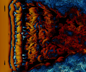
The growth and instability of the ILEV structures are first demonstrated through realisations of the streamwise velocity fields taken at the plane of symmetry of the leaflets (cf.  $z=0$ plane in figure 2). This plane cuts through the leaflets at their maximum chord length and is expected to exhibit the strongest ILEV instabilities, as it corresponds to the largest chord-to-thickness ratio. Three snapshots of the streamwise velocity are shown in figure 4. Various flow features are present. Laminar flow structures similar to Burgers vortices are first observed in the wake of the leaflets. Second, a complex form of shear-layer instabilities is observed in the sinus cavities. This instability only interacts with flow structures in the bulk flow near the centreline after the breakdown in that region has already started. Third, ILEV instabilities are observed downstream of the leading edges of both leaflets, and on their inner surfaces. We note that this latter instability mechanism creates strong flow disturbances which are convected downstream and interact with the other organised wake structures. The interaction of the disturbances created by the ILEV instability mechanism with the wake structures initiates the transition to turbulence in the wake (see the area within the dashed circle in figure 4). Finally, Falkner–Skan boundary layers on the outer sides of the leaflets seem to remain stable in the valve model.

Figure 4. Evolution of the streamwise velocity for the subset of flow field corresponding to the  $z=0$ plane. This plane cuts through the leaflets at their axis of symmetry. Snapshots, from left to right, are taken at $t=60,\ 96$ and $132\,{\rm ms}$ through the acceleration waveform (cf. figure 3). Dark red and dark blue regions show maximum and minimum velocities. Observed flow instabilities include, (i) laminar Burgers-like structures straining in the wake, (ii) 3-D instability in the cavities, (iii) stable Falkner–Skan-type boundary layers with favourable pressure gradients on the outer side of the valve leaflets, (iv) unstable ILEV on the inner sides of the leaflets and (v) nonlinear breakdown in the wake due to an interaction of the instabilities induced by the ILEV with the Burgers vortices in the wake.
Figure 5 shows the Lagrangian coherent structures around one valve leaflet. The flow field is taken at the peak flow  $t=200$ ms. Four stages of the flow instability are marked with labels LS, PR, SI and TWB, which stand for ‘laminar separation’, ‘primary rolls’, ‘secondary instabilities’ and ‘turbulent wake breakdown’, respectively. LS corresponds to the shear layer which separates at the leading edge (the laminar part of ILEV) and is inherently uniform in the spanwise direction. This verifies the planar assumption that was used for adopting the 2-D submodel in Zolfaghari & Obrist (Reference Zolfaghari and Obrist2019). It is further quantified here using velocity profiles in the central orifice and over the LS zone (figure 6), which show only small spanwise variations. PR marks the relatively narrow zone where primary instabilities appear on the separated shear layer. The resulting vortex seems to consist of essentially 2-D spanwise rolls. The SI zone shows the area where the primary rolls appearing on the ILEV undergo a secondary instability, triggering a predominantly 3-D dynamics. TWB shows the area where ILEV instabilities interact with the wake structures and create a turbulent state. We will focus on this ILEV instability and on designing possible control strategies to eliminate or attenuate this instability. Ideally, suppressing the primary instability mechanism would result in a laminar flow over the leaflet, and thereby reduce turbulence in the wake area. This was shown using a 2-D control case by Zolfaghari & Obrist (Reference Zolfaghari and Obrist2019). Here, we verify this effect in the 3-D model. We modify the leaflets’ leading edges in the $z=0$ plane the same way as in Zolfaghari & Obrist (Reference Zolfaghari and Obrist2019), and apply this modification homogeneously in the spanwise direction. Figure 7 shows that the control case results in a significantly lower oscillations in the wake flow. The cross-section profiles on the right side of this figure show that the elimination of ILEV has resulted in no oscillations in the central orifice.

Figure 5. Iso-surfaces of  $\lambda _2=-0.01$ coloured by the streamwise velocity, for a cuboid subset of the flow field encompassing one leaflet in the central orifice area ( $2r_h\le r\le 0$). Light yellow and light blue regions show maximum and minimum streamwise velocities, respectively. The red dashed line shows the leading edge, and the green dashed line shows the trailing edge. Four zones of flow instability are marked in the streamwise direction. LS denotes the laminar separation zone, which corresponds to a shear layer that is inherently uniform in the spanwise direction. PR shows the narrow extent over which primary rolls appear as a result of a primary ILEV instability. SI marks the approximate interval where primary rolls undergo a secondary instability and become rapidly three-dimensional. TWB shows the turbulent wake breakdown area, where ILEV instabilities interact with leaflet wake structures, causing a turbulent wake.

Figure 6. Small spanwise variations in velocity profiles inside the laminar extent of ILEV. Streamwise (black) and cross-stream (blue) velocity profiles are shown for three different spanwise locations  $z=0\,{\rm mm}, z=-4.5\,{\rm mm}$ and $z=-9\,{\rm mm}$ at $t=72\,{\rm ms}$.

Figure 7. Effect of ILEV instability on the wake turbulence: streamwise velocity on the  $r=0$ plane (left panels, which correspond to the dotted line on the right panels) and $x=0$ plane (right panels, which correspond to the dashed line on the left panels) at $t=84\,{\rm ms}$ are shown for the original BMHV design (top) and for the modified leaflet design (bottom). Significantly less wake oscillations are seen for the control case. The cross-sections in the right panels show no oscillatory flow in the central orifice for the control case.
3. Modal linear instability
3.1. Two-dimensional modal formulation for temporal instability
We investigate the global linear temporal stability of the time-averaged velocity profiles in the ILEV, as described in Zolfaghari & Obrist (Reference Zolfaghari and Obrist2019). To avoid issues of intractability of the associated eigenvalue problem, we focus on a subdomain covering the extent of the mean 2-D ILEV profile near one leaflet (figure 8). The mean ILEV flow is generated using the same 2-D DNS set-up presented in Zolfaghari & Obrist (Reference Zolfaghari and Obrist2019). Accordingly, the local ( $\xi,\eta$)-coordinate system described there is used here as well. Briefly recalling relevant details, $\xi$ denotes the streamwise axis with the origin at the leading edge of the leaflets, and $\eta$ represents the cross-stream axis which originates from the centreline and spans the space between the two leaflets. The $\eta$-axis then intersects the upper leaflet at $\eta ^*(\xi )$ and the lower leaflet at $-\eta ^*(\xi )$.

Figure 8. The local subdomain used for the global stability analysis. The grey lines show the background grid  $\tilde {\mathcal {G}}$. The true spatial resolution is three times higher than the finer grid patches illustrated near the leaflet boundary. The shaded subdomain represents the grid subset $\mathcal {W}$, for which the global matrices are formed. The grid points near the boundary (labelled as $\partial _{wall}$) are treated by the sharp-interface immersed boundary method. The local coordinate system ( $\xi,\eta$) used for the global instability analysis is also given. The origin of the streamwise axis $\xi$ is located at the leaflet's leading edge. The cross-stream axis $\eta$ extends from the centreline ( $\eta =0$) to the leaflet surface ( $\eta =\eta ^*(\xi )$) at each streamwise location $\xi$ (see red dashed line).
3.1.1. Governing equations
Decomposing the flow field at the leading edge  ${\tilde {\boldsymbol{\mathsf{q}}}}=({\tilde {\boldsymbol{\mathsf{u}}}},\tilde {p})$ into a mean flow ${{\tilde {\boldsymbol{\mathsf{Q}}}}}=({\tilde {\boldsymbol{\mathsf{u}}}},\tilde {P})$ and a perturbation ${\tilde {\boldsymbol{\mathsf{Q}}}^\prime }$ ( ${\tilde {\boldsymbol{\mathsf{Q}}}}={\tilde {\boldsymbol{\mathsf{Q}}}} +{\tilde {\boldsymbol{\mathsf{Q}}}^\prime }$; $\|{\tilde {\boldsymbol{\mathsf{q}}}^\prime } \|\ll \|{\tilde {\boldsymbol{\mathsf{q}}}}\|$) and substituting into the Navier–Stokes equations leads to the linearised Navier–Stokes equations which read
 \begin{equation} \partial_t{\tilde{\boldsymbol{\mathsf{u}}}^\prime}+{\tilde{\boldsymbol{\mathsf{u}}}^\prime}\boldsymbol{\cdot} \boldsymbol{\nabla}{\tilde{\boldsymbol{\mathsf{u}}}}+{\tilde{\boldsymbol{\mathsf{u}}}}\boldsymbol{\cdot} \boldsymbol{\nabla}{\tilde{\boldsymbol{\mathsf{u}}}^\prime}={-}\boldsymbol{\nabla}\tilde{p}^\prime+\frac{1}{Re_*}\nabla^2{\tilde{\boldsymbol{\mathsf{u}}}^\prime};\quad \boldsymbol{\nabla}\boldsymbol{\cdot}{\tilde{\boldsymbol{\mathsf{u}}}^\prime}=0. \end{equation}
Here,  $\tilde {\boldsymbol{\mathsf{U}}}$ denotes the 2-D time-averaged flow field obtained as
 \begin{equation} {{\tilde{\boldsymbol{\mathsf{U}}}}}(\xi,\eta) =\frac{1}{\boldsymbol{{\tilde{T}}}} \int^{t_0+\tilde{\boldsymbol{T}}}_{t_0} \frac{\tilde{\boldsymbol{\mathsf{u}}}(\xi,\eta,t)}{U_{{max},\xi=0}(t)}{\rm d} t. \end{equation}
The Reynolds number  $Re_*$ is based on the maximum streamwise velocity at the leading edge ( $\overline {U_{max,\xi =0}}$) as the reference velocity and the distance between the leaflets at the leading edge ( $\eta ^*_0=\eta ^*(\xi =0)$) as the reference length. We have
 \begin{equation} Re_* = \frac{{\overline{U_{max,\xi=0}}}\eta^*_0}{\nu}, \end{equation}
where
 \begin{equation} \overline{U_{max,\xi=0}} = \frac{1}{\tilde{\boldsymbol{{T}}}} \int^{t_0+\tilde{\boldsymbol{T}}}_{t_0}{U_{\text{max},\xi=0}(t)}\,{\rm d} t. \end{equation}
Introducing a global mode ansatz of the form  $\tilde {\boldsymbol{\mathsf{q}}}^\prime (\boldsymbol{\mathsf{x}},t)=\hat{\boldsymbol{\mathsf{q}}} (\boldsymbol{\mathsf{x}})\,{\rm e}^{-{\rm i}\tilde {\beta }t}$, where $\boldsymbol{\mathsf{x}}$ and $t$ denote the 2-D spatial coordinates and time, into the LNSE (3.1a,b) yields a system of partial differential equations (PDEs)
 \begin{equation} \begin{bmatrix} \mathscr{L}\{\tilde{\boldsymbol{\mathsf{u}}};Re_*\}+\tilde{U}_\xi & \tilde{U}_\eta & \mathscr{D}_\xi \\ \tilde{V}_\xi & \mathscr{L}\{\tilde{\boldsymbol{\mathsf{u}}};Re_*\} & \mathscr{D}_\eta \\ \mathscr{D}_\xi & \mathscr{D}_\eta & 0 \end{bmatrix} \begin{bmatrix} \hat{u} \\ \hat{v} \\ \hat{p} \end{bmatrix}= \mathrm{i}\tilde{\beta} \begin{bmatrix} 1 & 0 & 0 \\ 0 & 1 & 0 \\ 0 & 0 & 0 \end{bmatrix} \begin{bmatrix} \hat{u} \\ \hat{v} \\ \hat{p} \end{bmatrix} \end{equation}
where  $\mathscr {L}\{\boldsymbol {\tilde {U}};Re_*\}=\tilde {U}\mathscr {D}_\xi +\tilde {V}\mathscr {D}_\eta -1/Re_*(\mathscr {D}_{\xi \xi }+\mathscr {D}_{\eta \eta })$, and $\skew2\hat{{\boldsymbol{\mathsf{q}}}}=(\hat{{\boldsymbol{\mathsf{u}}}},\hat {{p}})$ with the velocity vector ${{\hat{{\boldsymbol{\mathsf{u}}}}}}=({\hat {u}},\hat {{v}})$. In the above expression $\mathscr {D}_\xi$ and $\mathscr {D}_{\xi \xi }$ denote the first and second derivatives with respect to the $\xi$-direction, respectively.
Temporal global modes with  $\operatorname {Im}\{\tilde {\beta }\}>0$ are sought. To this end, we discretise (3.5) using second-order finite-differences with $n_p=123\,71$ grid points. This results in a complex generalised eigenvalue problem of the form
 \begin{equation} \boldsymbol{\mathsf{A}}_{3n_p\times 3n_p}(Re_*,{\tilde{\boldsymbol{\mathsf{u}}}}) \boldsymbol{\hat{\boldsymbol{\mathsf{q}}}}_{3n_p\times 1}=\mathrm{i}\tilde{\beta} \boldsymbol{\mathsf{B}}_{3n_p\times 3n_p}\boldsymbol{\hat{\boldsymbol{\mathsf{q}}}}_{3n_p\times 1}, \end{equation}
where  $\boldsymbol{\hat{\boldsymbol{\mathsf{q}}}}$ is the discretised form of $\hat{{\boldsymbol{\mathsf{q}}}}$.
3.1.2. Integration of the immersed boundaries
The sharp-interface immersed boundary method (Mittal et al. Reference Mittal, Dong, Bozkurttas, Najjar, Vargas and von Loebbecke2008) is used to integrate the boundary conditions associated with the leaflet walls into the matrices  $\boldsymbol{\mathsf{A}}$ and $\boldsymbol{\mathsf{B}}$ (see (3.6)). The workflow of labelling the grid points according to their position with respect to the boundaries is demonstrated in algorithm 1. Compatibility boundary conditions for pressure are imposed on the domain's inlet and outlet as well as on the solid walls. These conditions, in general, read
 \begin{equation} \boldsymbol{\nabla}\tilde{p}^\prime={-}{\tilde{\boldsymbol{\mathsf{u}}}} \boldsymbol{\cdot}\boldsymbol{\nabla}{\tilde{\boldsymbol{\mathsf{u}}}^\prime}+\frac{1}{Re_*}\nabla^2{\tilde{\boldsymbol{\mathsf{u}}}^\prime}. \end{equation}
On the leaflet walls, this condition simplifies since  $\tilde {\boldsymbol{\mathsf{U}}}=\boldsymbol{\mathsf{0}}$, and (3.7) reduces to
 \begin{equation} \boldsymbol{\nabla}\tilde{p}^\prime=\frac{1}{Re_*}\nabla^2{{\tilde{\boldsymbol{\mathsf{u}}}^\prime}}. \end{equation}
The compatibility boundary conditions, together with zero-disturbance Dirichlet boundary conditions for the velocity vector given by
 \begin{equation} \tilde{\boldsymbol{\mathsf{u}}}^\prime(\boldsymbol{\mathsf{x}},t)=0,\quad \boldsymbol{\mathsf{x}}\in{\partial_{in}\cup \partial_{walls}\cup\partial_{out} \cup\partial_\infty}, \end{equation}
are discretised and integrated into the matrices  $\boldsymbol{\mathsf{A}}$ and $\boldsymbol{\mathsf{B}}$. To save computational time, and owing to the symmetry of the velocity profiles, only half of the profile is considered, which is results in a symmetry boundary condition at $\tilde {\eta } = 0$.
Algorithm 1 Two-dimensional global instability solver with immersed boundaries

Figure 9 shows the real part of the streamwise velocity component of the two zero-frequency global eigenmodes with positive temporal growth rates. Mode A, which has a higher growth rate, has a similar spatial structure than the one found for X-junction flow (Lashgari et al. Reference Lashgari, Tammisola, Citro, Juniper and Brandt2014), stretching from the separation point to the trailing end of the wave-maker zone. This could be related to similarities in the two base flows: both include flow separation downstream of a sharp edge. Yet, our mode presents more waviness past the wave maker, which includes the area where the separated shear layer reattaches. This waviness may be attributed to the strong fluctuations that are observed over the reattachment zone of ILEV structures, which were also reported by Cherry, Hillier & Latour (Reference Cherry, Hillier and Latour1984). Mode B, on the other hand, is more concentrated near the leading edge of the wave-maker zone. It slowly emerges on the separated shear layer nearly two thickness lengths downstream of the leading edge, and vanishes towards the reattachment zone. Provided this mode is present where the shear layer has the highest reverse-to-forward flow ratio, it projects the dynamics of the shear layer seemingly uninfluenced by the presence of the wall. This is in contrast to mode A, where oscillatory effects can be observed at locations where this latter ratio is low. In line with this, mode A includes a wavy structure that is extended to the outflow boundary, before it is affected by the homogeneous Dirichlet boundary conditions there. We will show in Appendix A that the structure of this mode and mode B (as well as their associated eigenvalues) do not change when the outflow boundary is extended further downstream.

Figure 9. Global modes (a) A and (b) B, visualised by the real part of the streamwise velocity component. Dashed lines mark the extent of the local absolute instability. Approximate separation streamlines for the mean flow are drawn as solid black lines. Dark red and dark blue colours indicate the colour map extrema.
3.2. Structural sensitivity of the linear global modes
3.2.1. Adjoint modal formulation
For investigating the sensitivity of the global modes characteristics (e.g. their growth rates) to the underlying flow, adjoints of the global modes are studied. For the pairs  $(\tilde {\boldsymbol{\mathsf{u}}}^\prime,\tilde {p}^\prime )$ and $(\tilde {\boldsymbol{\mathsf{u}}}^{\prime,{\dagger} },\tilde {p}^{\prime,{\dagger} })$ the following Lagrange identity holds as:
 \begin{equation} {[\mathscr{P}\boldsymbol{\cdot} \tilde{\boldsymbol{\mathsf{u}}}^{\prime,{\dagger}} + \boldsymbol{\nabla}\boldsymbol{\cdot} \tilde{\boldsymbol{\mathsf{u}}}^\prime \tilde{p}^{\prime,{\dagger}}]} + {[\tilde{\boldsymbol{\mathsf{u}}}^\prime\boldsymbol{\cdot}\mathscr{P}^{\dagger}{+} \boldsymbol{\nabla} \boldsymbol{\cdot}\tilde{\boldsymbol{\mathsf{u}}}^{\prime,{\dagger}} {\tilde{p}}^\prime]}= \partial_t (\tilde{\boldsymbol{\mathsf{u}}}^\prime\boldsymbol{\cdot}\tilde{\boldsymbol{\mathsf{u}}}^{\prime,{\dagger}}) + \boldsymbol{\nabla}\boldsymbol{\cdot} \boldsymbol{\mathsf{M}}^{\dagger}, \end{equation}
where
 \begin{equation} \mathscr{P} \{\tilde{\boldsymbol{\mathsf{u}}}^\prime,{\tilde{p}^{\prime}}, \tilde{\boldsymbol{\mathsf{u}}}, Re_*\} = \partial_t \tilde{\boldsymbol{\mathsf{u}}}^\prime+ \tilde{\boldsymbol{\mathsf{u}}} \boldsymbol{\cdot}\boldsymbol{\nabla}\tilde{\boldsymbol{\mathsf{u}}}^\prime + \tilde{\boldsymbol{\mathsf{u}}}^\prime\boldsymbol{\cdot}\boldsymbol{\nabla} \tilde{\boldsymbol{\mathsf{u}}}+ \boldsymbol{\nabla} {\tilde{p}}^\prime-\frac{1}{Re_*}\nabla^2 \tilde{\boldsymbol{\mathsf{u}}}^{\prime,{\dagger}},\end{equation}
and
 \begin{equation} \mathscr{P}^{\dagger}\{ \tilde{\boldsymbol{\mathsf{u}}}^{\prime,{\dagger}},{\tilde{p}^{\prime,{\dagger}}}, \tilde{\boldsymbol{\mathsf{u}}}, Re_*\}= \partial_t \tilde{\boldsymbol{\mathsf{u}}}^{\prime,{\dagger}}+ \tilde{\boldsymbol{\mathsf{u}}}\boldsymbol{\cdot}\boldsymbol{\nabla} \tilde{\boldsymbol{\mathsf{u}}}^{\prime,{\dagger}} - \tilde{\boldsymbol{\mathsf{u}}}^{\prime,{\dagger}} \boldsymbol{\cdot} (\boldsymbol{\nabla} \tilde{\boldsymbol{\mathsf{u}}})^{\rm T}+ \boldsymbol{\nabla} \tilde{p}^{\prime,{\dagger}} + \frac{1}{Re_*}\nabla^2 \tilde{\boldsymbol{\mathsf{u}}}^{\prime,{\dagger}}. \end{equation}
Here,  $\boldsymbol{\mathsf{M}}^{\dagger}$ is the bilinear concomitant defined as
 \begin{equation} \boldsymbol{\mathsf{M}}^{\dagger}{=}\tilde{\boldsymbol{\mathsf{u}}} (\tilde{\boldsymbol{\mathsf{u}}}^\prime\boldsymbol{\cdot}\tilde{\boldsymbol{\mathsf{u}}}^{\prime,{\dagger}})+ \frac{1}{Re_*}(\boldsymbol{\nabla} \tilde{\boldsymbol{\mathsf{u}}}^{\prime,{\dagger}}\boldsymbol{\cdot} \tilde{\boldsymbol{\mathsf{u}}}^\prime- \boldsymbol{\nabla} \tilde{\boldsymbol{\mathsf{u}}}^\prime\boldsymbol{\cdot} \tilde{\boldsymbol{\mathsf{u}}}^{\prime,{\dagger}})+\tilde{p}^{\prime,{\dagger}} \tilde{\boldsymbol{\mathsf{u}}}^\prime+{\tilde{p}}^\prime \tilde{\boldsymbol{\mathsf{u}}}^{\prime,{\dagger}}. \end{equation}
Integrating the Lagrange identity over the entire domain and over the chosen time horizon and using the divergence theorem for the last term, we obtain the adjoint LNSE in the form
 \begin{equation} \mathscr{P}^{\dagger}\{ \tilde{\boldsymbol{\mathsf{u}}}^{\prime,{\dagger}},{\tilde{p}^{\prime,{\dagger}}}, \tilde{\boldsymbol{\mathsf{u}}}, Re_*\} =0;\quad \boldsymbol{\nabla}\boldsymbol{\cdot} \tilde{\boldsymbol{\mathsf{U}}}^{\prime,{\dagger}}=0. \end{equation}
Fourier transformation of (3.10) using the ansatz  ${\tilde {\boldsymbol{\mathsf{q}}}}^{\prime,{\dagger} } (\boldsymbol{\mathsf{x}},t)= \hat{{\boldsymbol{\mathsf{q}}}}^{\dagger} (\boldsymbol{\mathsf{x}}) \,{\rm e}^{-\mathrm {i}\tilde {\beta }^{\dagger} t}$, where $\boldsymbol{\mathsf{x}}$ and $t$ are the 2-D spatial coordinates and time, gives the coupled form of the adjoint LNSE
 \begin{align} \begin{bmatrix} \mathscr{L}^{\dagger}{\{\tilde{\boldsymbol{\mathsf{u}}};Re_*\}} - \partial_\xi\tilde{U} & - \partial_\xi\tilde{V} & \mathscr{D}_\xi \\ -\partial_\eta\tilde{U} & \mathscr{L}^{\dagger}{\{\tilde{\boldsymbol{\mathsf{u}}}; Re_*\}}-\partial_\eta\tilde{V} & \mathscr{D}_\eta \\ \mathscr{D}_\xi & \mathscr{D}_\eta & 0 \end{bmatrix} \begin{bmatrix} \hat{u}^{\dagger} \\ \hat{v}^{\dagger} \\ \hat{p}^{\dagger} \end{bmatrix} =\mathrm{i}\tilde{\beta}^{\dagger} \begin{bmatrix} 1 & 0 & 0 \\ 0 & 1 & 0\\ 0 & 0 & 0 \end{bmatrix} \begin{bmatrix} \hat{u} ^{\dagger} \\ \hat{v} ^{\dagger} \\ \hat{p} ^{\dagger} \end{bmatrix}, \end{align}
where  $\mathscr {L}^{\dagger} {\{\tilde {\boldsymbol{\mathsf{u}}};Re_*\}}= \tilde {U}\mathscr {D}_\xi +\tilde {V}\mathscr {D}_\eta +Re_*^{-1}(\mathscr {D}_{\xi \xi }+\mathscr {D}_{\eta \eta })$, ${\hat{ {\boldsymbol{\mathsf{q}}}}^{{\dagger} }}= (\hat{{\boldsymbol{\mathsf{u}}}}^{\dagger},\hat {{p}}^{{\dagger} })$ and ${\hat{{\boldsymbol{\mathsf{u}}}}^{{\dagger} }}=({\hat {u}}^{\dagger},\hat {{v}}^{{\dagger} })$. The operators $\mathscr {D}_{\xi }$ and $\mathscr {D}_{\xi \xi }$ denote the first and second derivatives with respect to $\xi$, respectively. Discretisation yields the generalised eigenvalue problem
 \begin{equation} \boldsymbol{\mathsf{A}}^{\dagger}_{3n_p\times 3n_p}({\tilde{\boldsymbol{\mathsf{U}}}},Re_*) \boldsymbol{\hat{\boldsymbol{\mathsf{q}}}}^{\dagger}_{3n_p\times 1}=\mathrm{i}{\tilde{\beta}}^{\dagger} \boldsymbol{\mathsf{B}}^{\dagger}_{3n_p\times 3n_p}({\tilde{\boldsymbol{\mathsf{U}}}},Re_*) \boldsymbol{\hat{\boldsymbol{\mathsf{q}}}}^{\dagger}_{3n_p\times 1}, \end{equation}
where  $\boldsymbol{\hat{\boldsymbol{\mathsf{q}}}}^{\dagger}$ is the discretised form of adjoint state vector. Homogeneous Dirichlet boundary conditions for the adjoint velocity disturbances $\tilde {\boldsymbol{\mathsf{u}}}^{\prime,{\dagger} }$ are applied, together with compatibility boundary condition for the adjoint pressure disturbance $\tilde {p}^{\prime,{\dagger} }$. The compatibility boundary conditions for $\tilde {p}^{\prime,{\dagger} }$ prove to be the proper choice for the domain's inflow and outflow. To obtain the adjoint compatibility boundary conditions, we first substitute this condition for the direct problem (3.7) into the momentum component of the direct linearised Navier–Stokes equations (3.1a,b). This yields
 \begin{equation} \partial_t{{\tilde{\boldsymbol{\mathsf{u}}}^\prime}}+{{\tilde{\boldsymbol{\mathsf{u}}}^\prime}}\boldsymbol{\cdot} \boldsymbol{\nabla}{{\tilde{\boldsymbol{\mathsf{U}}}}}=0, \end{equation}
which, in the adjoint form, becomes
 \begin{equation} \partial_t{{\tilde{\boldsymbol{\mathsf{u}}}^{\prime,{\dagger}}}}+{{\tilde{\boldsymbol{\mathsf{U}}}}} \boldsymbol{\cdot}\boldsymbol{\nabla}\tilde{\boldsymbol{\mathsf{u}}}^{\prime,{\dagger}}=0. \end{equation}
Equation (3.18) is incorporated into  $\boldsymbol{\mathsf{A}}^{\dagger}$ and $\boldsymbol{\mathsf{B}}^{\dagger}$ at the inflow, centreline, and outflow locations, where $\tilde {\boldsymbol{\mathsf{U}}}\neq \boldsymbol{\mathsf{0}}$.
Figure 10 shows the adjoint global modes corresponding to the direct global modes A and B. The adjoint modes can be used to quantify the sensitivity of the global direct modes to external forcing (Giannetti & Luchini Reference Giannetti and Luchini2007). We use both direct and adjoint modes for constructing the structural sensitivity tensor which can be used to guide the stabilisation of these modes.

Figure 10. Adjoint global modes (a) A and (b) B, visualised by the streamwise velocity component. Dashed lines mark the extent of the local absolute instability. Approximate separation streamlines for the mean flow are drawn as solid black lines. Dark red and dark blue colours indicate the colour map extrema. Larger magnitudes correspond to higher sensitivities of the global modes to the underlying flow.
3.2.2. Structural sensitivity to a local feedback source
We follow the localised momentum feedback approach pioneered by Hill (Reference Hill1992) and Giannetti & Luchini (Reference Giannetti and Luchini2007). We perturb the momentum equation of the LNSE, after Fourier decomposition in time, by the linear operator  $\delta \mathscr {M}$
 \begin{equation} \left.\begin{gathered} \tilde{\beta}^\prime \hat{{\boldsymbol{\mathsf{u}}}}^{\prime} + \mathscr{L}^+\{\tilde{\boldsymbol{\mathsf{U}}},Re_*\}\hat{{\boldsymbol{\mathsf{u}}}}^{\prime}+ \boldsymbol{\nabla}\hat{p}^{\prime}=\boldsymbol{\delta}\mathscr{M}(\hat{{\boldsymbol{\mathsf{u}}}}^{\prime},\hat{p}^{\prime}) \\ \boldsymbol{\nabla}\boldsymbol{\cdot}\hat{{\boldsymbol{\mathsf{u}}}}^{\prime}=0, \end{gathered}\right\}, \end{equation}
where the  $\mathscr {L}^+$ operator is given as
 \begin{equation} \mathscr{L}^+\{{\tilde{\boldsymbol{\mathsf{U}}}}, Re_*\}\hat{{\boldsymbol{\mathsf{u}}}}^{\prime}= \hat{{\boldsymbol{\mathsf{u}}}}^{\prime}\boldsymbol{\cdot}\boldsymbol{\nabla} \tilde{\boldsymbol{\mathsf{U}}}+\tilde{\boldsymbol{\mathsf{U}}} \boldsymbol{\cdot}\boldsymbol{\nabla}\hat{{\boldsymbol{\mathsf{u}}}}^{\prime} -\frac{1}{Re_*}\nabla^2 \hat{{\boldsymbol{\mathsf{u}}}}^{\prime}. \end{equation}
Given the eigenvalue drift  $\delta \tilde {{\beta }}$ and the perturbation eigenmode $(\delta \hat{{\boldsymbol{\mathsf{u}}}},\delta \hat {p})$, where $\hat{ {\boldsymbol{\mathsf{u}}}}^{\prime }=\hat{ {\boldsymbol{\mathsf{u}}}}+\delta \hat{{\boldsymbol{\mathsf{u}}}}$, $\hat {{p}}^{\prime }=\hat {{p}}+\delta \hat {{p}}$ and ${\tilde {\beta }}^\prime ={\tilde {\beta }}+\delta {\tilde {\beta }}$, we arrive at
 \begin{equation} \left.\begin{gathered} \tilde{\beta} \delta\hat{{\boldsymbol{\mathsf{u}}}} + \mathscr{L}^+\{\tilde{\boldsymbol{\mathsf{U}}},Re_*\}\delta\hat{{\boldsymbol{\mathsf{u}}}}+ \boldsymbol{\nabla}\delta\hat{p}={-}\delta{\tilde{\beta}} \hat{{\boldsymbol{\mathsf{u}}}} +{{{\delta}}}\mathscr{M}(\hat{{\boldsymbol{\mathsf{u}}}},\hat{p})\\ \boldsymbol{\nabla}\boldsymbol{\cdot}\delta\hat{{\boldsymbol{\mathsf{u}}}}=0, \end{gathered}\right\} \end{equation}
using the Lagrange identity (similar to (3.10)) for  $(\delta \hat{{\boldsymbol{\mathsf{u}}}},\delta \hat {p})$ and $(\hat{ {\boldsymbol{\mathsf{u}}}}^{{\dagger} },\hat {p}^{{\dagger} })$. Taking $\delta \mathscr {M} = \boldsymbol{\mathsf{K}}\hat{{\boldsymbol{\mathsf{u}}}} \delta _{\boldsymbol{\mathsf{D}}}(\xi -\xi _+,\eta -\eta _+)$ and integrating over the entire computational domain, one obtains
 \begin{equation} \delta\tilde{\beta}=\frac{\langle \hat{{\boldsymbol{\mathsf{u}}}}^{{{\dagger}}} \boldsymbol{\cdot} \delta\mathscr{M}\rangle}{\langle\hat{{\boldsymbol{\mathsf{u}}}}\boldsymbol{\cdot} \hat{{\boldsymbol{\mathsf{u}}}}^{{{\dagger}}} \rangle}= \frac{\langle\hat{{\boldsymbol{\mathsf{u}}}}^{{{\dagger}}}\boldsymbol{\cdot}\boldsymbol{\mathsf{K}} \hat{{\boldsymbol{\mathsf{u}}}}\delta_{\boldsymbol{\mathsf{D}}}(\xi-\xi_+,\eta-\eta_+)\rangle} {\langle\hat{{\boldsymbol{\mathsf{u}}}}\boldsymbol{\cdot}\hat{{\boldsymbol{\mathsf{u}}}}^{{{\dagger}}} \rangle} = \frac{\kappa_0\hat{{\boldsymbol{\mathsf{u}}}}(\xi_+,\eta_+)\hat{{\boldsymbol{\mathsf{u}}}}^{{{\dagger}}} (\xi_+,\eta_+)}{\langle\hat{{\boldsymbol{\mathsf{u}}}}\boldsymbol{\cdot}\hat{{\boldsymbol{\mathsf{u}}}}^{{{\dagger}}} \rangle}. \end{equation}
In the above formulation,  $\delta _{\boldsymbol{\mathsf{D}}}$ is the Dirac delta function, $\langle \cdot \rangle$ is the integral over the computational domain and $\boldsymbol{\mathsf{K}}$ and $\kappa _0=\boldsymbol{\mathsf{K}}(\xi _+,\eta _+)$ indicate the strength of the momentum feedback on the entire domain and at point $(\xi _+, \eta _+)$, respectively. It follows that the response of each component of momentum feedback on the growth rate and frequency of the global modes can be realised by assessing the real and imaginary parts of the sensitivity tensor $\boldsymbol{\mathsf{S}}=\hat{{\boldsymbol{\mathsf{u}}}} \otimes \hat{{\boldsymbol{\mathsf{u}}}}^{\dagger}$, which consists of the dyadic product of the direct and adjoint velocity modes. The imaginary part of the components of $\boldsymbol{\mathsf{S}}$ measure the sensitivity of the global mode with respect to the growth rate, while the real part determines the sensitivity with respect to the frequency. Here, we focus on the imaginary part, as we are interested in stabilisation of the modes, hoping to eliminate the vortex shedding between and downstream of the leaflets of the BMHV.
The components of the sensitivity tensor associated with modes A and B are given in figures 11 and 12. For mode A, the highest sensitivities are generally concentrated in the wave-maker zone. This is not surprising as a local absolute instability is defined by an instability with infinite impulse response at a fixed location. A feedback, if sufficiently small to preserve the instability characteristics of the base flow, could be seen in extreme cases as an input, which will be maximally amplified in the wave-maker zone. In terms of different components of sensitivity,  $S_{12}=\hat {u}\hat {v}^{\dagger}$ appears to have a slightly higher magnitude than other components. This implies that, within a linear regime, a forcing in the cross-stream direction will trigger the largest response in the streamwise component of the direct mode. This could be explained by further investigating the characteristics of the base flow, such as the properties of the rate of strain tensor, but such an analysis will be postponed to a future effort. For mode B, the maximum structural sensitivity occurs upstream and almost completely outside the wave-maker zone. This observation signals a large influence of the base flow on the dynamics of this shear-layer mode, possibly through a feedback mechanism supported by recirculation.

Figure 11. Components of the sensitivity tensor  $\boldsymbol{\mathsf{S}}$ for mode A. Yellow areas denote the maximum, blue areas denote the minimum sensitivity. The domain between the dashed white lines is locally absolutely unstable.

Figure 12. Components of the sensitivity tensor  $\boldsymbol{\mathsf{S}}$ for mode B. Yellow areas denote the maximum, blue areas denote the minimum sensitivity. The domain between the dashed white lines is locally absolutely unstable (wave-maker region).
3.2.3. Passive control based on localised feedback
Motivated by the original experimental work of Strykowski & Sreenivasan (Reference Strykowski and Sreenivasan1990) and the follow-up theoretical study of Hill (Reference Hill1992) who tried to suppress the first instability of cylinder wake flow at  $Re\approx 50$ by introducing localised roughness elements into the system, we use this technique to try to suppress the ILEV instabilities in the BMHVs. Several differences exist between the two cases, the most importantly, the two orders of magnitude larger Reynolds number of the BMHV flow compared with the cylinder wake flow. It is also not clear whether a localised feedback will strengthen, or weaken the instability. Besides, given that more than one global mode is involved, with high structural sensitivities in distinct locations, the likelihood that only one feedback source may eliminate the instability entirely is likely small. It is also important to note that, because the Reynolds number is relatively high in our case, a localised feedback, positioned relatively far from the wall may cause more instability, e.g. via introducing von-Kármán-type vortex streets. Despite these apprehensions, we nonetheless put our findings from the linear structural sensitivity analysis to the test by performing 2-D DNSs. We introduce small feedback sources in the form of small cylinders (far from the wall, for mode A), or in the form of a semicircular bump (close to the wall, for mode B), and perform 2-D DNS using the parameters from Zolfaghari & Obrist (Reference Zolfaghari and Obrist2019). For mode A, we observed that a localised feedback did not seem to improve the flow scenario (not shown). The inserted cylinder near the upstream end of the wave-maker zone created instabilities which evolved into travelling vortices downstream of the feedback source. Given that mode B was not triggered, it induced waviness in the ILEV which interacted with the instabilities created by the cylinder. For mode B, we anticipated a more positive outcome, as this mode has a more localised sensitivity compared with mode A. This localised area is closer to the wall which, due to lower velocities and a smaller surface, generates less drag force on the original base flow. Thus, the base flow characteristics are likely to change less than for mode A. Significant changes in the base flow $\tilde {\boldsymbol{\mathsf{U}}}$ may render the structural sensitivity analysis invalid, because the eigenvalue shift $\delta \beta$ based on (3.22) assumes small and thus negligible changes in the base flow. A better outcome is also expected because the area to be triggered lies outside the absolute instability zone. For this reason, the chances of triggering more instabilities by the large impulse response of the wave maker are rather low.
Figure 13 shows the outcome of passive control via local feedback associated with mode B. For the local feedback, two small and equal circular bumps with a radius of  $R_c=0.126$ mm were added on both leaflet surfaces at $\xi _c=4.95$ and $\eta _c=\pm 1.68$ mm. The positions of these bumps were chosen to be approximately in the centre of the maximum sensitivity area for mode B. It can be observed that with passive control the vorticity production between the leaflets was diminished, but not eliminated. In more detail, as shown using instantaneous vorticity fields, the location where first vortices, forming due to ILEV instabilities, detach into the bulk flow could be moved downstream by nearly one third of a chord length. Thanks to this improvement, the mutual interaction between the vortices, generated by ILEVs and forming on the top and bottom leaflets, was nearly eliminated. In general, even though the ILEV instability could not be fully controlled, this passive control device resulted in a noticeably less chaotic wake flow past the valve. This is further quantified in figure 14 using area-normalised enstrophy defined as
 \begin{equation} \boldsymbol{E}_S(\pmb{\omega})= \frac{1}{S}\int_S\pmb{\omega}\boldsymbol{\cdot}\pmb{\omega}\,{\rm d} S, \end{equation}
where  $\pmb {\omega }=\boldsymbol {\nabla }\times \boldsymbol{\mathsf{u}}$ is the vorticity and $S$ indicates the circular area where the integration is performed. Significantly lower enstrophy is found for the control case both within the central orifice and in the wake, which demonstrates the efficacy of the control.

Figure 13. Instantaneous vorticity for (a) baseline ILEV flow and (b) ILEV flow with local feedback control corresponding to mode B.

Figure 14. Effect of passive control based on momentum feedback on normalised enstrophy  $\boldsymbol {E}_S(\pmb {\omega })$ at ((a), in central orifice) 5.76 mm and ((b), in the wake) 12.96 mm downstream of the leading edge. The integration area $S$ was a circle of radius 3.6 mm and centred on $r=0$ mm.
4. Disturbance energy growth analysis
The hydrodynamic stability analyses performed in the previous section and by Zolfaghari & Obrist (Reference Zolfaghari and Obrist2019) were asymptotic and focused on the ILEV zone of the BMHV flow. While this type of analysis is useful for understanding the instability mechanism itself, the influence of the ILEV instability on disturbance energy growth farther from its origin is also worth investigating. Zolfaghari & Obrist (Reference Zolfaghari and Obrist2019) showed by a geometry modification that the ILEV instability plays a key role in the laminar–turbulent transition of the valve wake. Without this modification, it would have been difficult to distinguish between ILEV instabilities and other mechanisms, e.g. the wake instability or driving by the cavities. Ideally, the strongest mechanism contributing to transition in a certain location, such as the wake, should be identified and analysed. In addition, the influence of various mechanisms is mostly time dependent, with the disturbance energy growth at a given location being driven by local mechanisms over shorter times. In the following, we formulate a linear gradient-based approach (Schmid Reference Schmid2007; Schmid, de Pando & Peake Reference Schmid, de Pando and Peake2017) to study the contribution of the ILEV instabilities at arbitrary locations and over given short-time horizons.
4.1. Direct non-modal formulation
4.1.1. Governing equations
We again consider the incompressible Navier–Stokes equations for a disturbance  $(\tilde {\boldsymbol{\mathsf{u}}}^\prime,{\tilde {p}}^\prime )$ around a global mean flow $(\tilde {\boldsymbol{\mathsf{U}}},\tilde {\boldsymbol{\mathsf{P}}})$,
 \begin{equation} \partial_t{{\tilde{\boldsymbol{\mathsf{u}}}}^\prime}+ {{\tilde{\boldsymbol{\mathsf{u}}}}^\prime}\boldsymbol{\cdot} \boldsymbol{\nabla}{{\tilde{\boldsymbol{\mathsf{U}}}}}+{{\tilde{\boldsymbol{\mathsf{U}}}}} \boldsymbol{\cdot}\boldsymbol{\nabla}{\tilde{\boldsymbol{\mathsf{u}}}^\prime}={-}\boldsymbol{\nabla}\tilde{p}^\prime+ \frac{1}{Re}\nabla^2{{\tilde{\boldsymbol{\mathsf{u}}}}^\prime};\quad \boldsymbol{\nabla}\boldsymbol{\cdot}{{\tilde{\boldsymbol{\mathsf{u}}}}^\prime}=0, \end{equation}
and seek to recover the ILEV instabilities as disturbances superimposed on a mean flow  $\tilde {\boldsymbol{\mathsf{U}}}$ at each time $t$. Note that we use a different mean flow for the nonlinear non-modal analysis than for the earlier linear modal approach give in (3.1a,b). Here, $\tilde {\boldsymbol{\mathsf{U}}}$ is obtained by temporally averaging of the velocity field $\tilde {\boldsymbol{\mathsf{u}}};$ no scaling is involved, and the averaging is performed over the entire flow domain. We have
 \begin{equation} {{{{\tilde{\boldsymbol{\mathsf{U}}}}}}}(x,r) = \frac{1}{\tilde{\boldsymbol{{T}}}}\int^{t_0+\tilde{\boldsymbol{T}}}_{t_0} {\tilde{\boldsymbol{\mathsf{u}}}(x,r,t)}\,{\rm d} t, \end{equation}
which also implies that the statistical averaging is performed over the global  $(x,r)$ instead of the local $(\xi,\eta )$ coordinates. The time-averaged flow field around the ILEV is shown in figure 15.

Figure 15. Time-averaged (a) streamwise and (b) cross-stream velocity components around the ILEV in the BMHV.
4.2. Adjoint equations with focus on arbitrary geometric energy masks
In order to study the optimal perturbations for maximising energy growth in specific locations within the computational domain (e.g. around the ILEV zone, or in the wake) we formulate the Lagrangian
 \begin{align} \mathcal{L} &=
\underbrace{\frac{1}{2}\left\langle
\mathscr{G}{\tilde{\boldsymbol{\mathsf{u}}}}^\prime
(\boldsymbol{\mathsf{x}},T) \cdot
\mathscr{G}\tilde{\boldsymbol{\mathsf{u}}}^\prime
(\boldsymbol{\mathsf{x}},T)
\right\rangle}_{\mathcal{J}_{\mathscr{G}}} + \phi
\left\{\frac{1}{2}\left\langle
\tilde{\boldsymbol{\mathsf{u}}}^\prime
(\boldsymbol{\mathsf{x}},0) \cdot
\tilde{\boldsymbol{\mathsf{u}}}^\prime
(\boldsymbol{\mathsf{x}},0)
\right\rangle-E_0\right\}\nonumber\\ &\quad + \int_0^{\rm
T} \left\langle
\tilde{\boldsymbol{\mathsf{u}}}^{\prime,\ddagger}\boldsymbol{\cdot}
\{\partial_t\tilde{\boldsymbol{\mathsf{u}}}^\prime
+\tilde{\boldsymbol{\mathsf{u}}}^\prime
\boldsymbol{\cdot}\boldsymbol{\nabla}\tilde{\boldsymbol{\mathsf{U}}}+\!
\tilde{\boldsymbol{\mathsf{U}}}
\boldsymbol{\cdot}\boldsymbol{\nabla}
\tilde{\boldsymbol{\mathsf{u}}}^\prime \!+\!
\boldsymbol{\nabla}\tilde{p}^\prime- Re^{{-}1}\nabla^2
\tilde{\boldsymbol{\mathsf{u}}}^\prime\}\right\rangle
{\rm d} t +\!\int_0^{\rm T} \left\langle
\tilde{p}^{\prime,\ddagger}\boldsymbol{\nabla}\boldsymbol{\cdot}
\tilde{\boldsymbol{\mathsf{u}}}^\prime\right\rangle
{\rm d} t, \end{align}
\begin{align} \mathcal{L} &=
\underbrace{\frac{1}{2}\left\langle
\mathscr{G}{\tilde{\boldsymbol{\mathsf{u}}}}^\prime
(\boldsymbol{\mathsf{x}},T) \cdot
\mathscr{G}\tilde{\boldsymbol{\mathsf{u}}}^\prime
(\boldsymbol{\mathsf{x}},T)
\right\rangle}_{\mathcal{J}_{\mathscr{G}}} + \phi
\left\{\frac{1}{2}\left\langle
\tilde{\boldsymbol{\mathsf{u}}}^\prime
(\boldsymbol{\mathsf{x}},0) \cdot
\tilde{\boldsymbol{\mathsf{u}}}^\prime
(\boldsymbol{\mathsf{x}},0)
\right\rangle-E_0\right\}\nonumber\\ &\quad + \int_0^{\rm
T} \left\langle
\tilde{\boldsymbol{\mathsf{u}}}^{\prime,\ddagger}\boldsymbol{\cdot}
\{\partial_t\tilde{\boldsymbol{\mathsf{u}}}^\prime
+\tilde{\boldsymbol{\mathsf{u}}}^\prime
\boldsymbol{\cdot}\boldsymbol{\nabla}\tilde{\boldsymbol{\mathsf{U}}}+\!
\tilde{\boldsymbol{\mathsf{U}}}
\boldsymbol{\cdot}\boldsymbol{\nabla}
\tilde{\boldsymbol{\mathsf{u}}}^\prime \!+\!
\boldsymbol{\nabla}\tilde{p}^\prime- Re^{{-}1}\nabla^2
\tilde{\boldsymbol{\mathsf{u}}}^\prime\}\right\rangle
{\rm d} t +\!\int_0^{\rm T} \left\langle
\tilde{p}^{\prime,\ddagger}\boldsymbol{\nabla}\boldsymbol{\cdot}
\tilde{\boldsymbol{\mathsf{u}}}^\prime\right\rangle
{\rm d} t, \end{align}
where  $\mathcal {J}_{\mathscr {G}}$ is an objective equipped with a sharp-interface geometric mask function $\mathscr {G}:\varOmega \to \varOmega _v$, which projects the global flow field onto the subdomain of interest $\varOmega _v$. This function is used to focus the optimisation procedure on the disturbance kinetic energy within $\varOmega _v$, which is moved over various areas of interest such as the wake and the trailing edge, to inspect the potential role of ILEV instabilities. The pair $(\tilde {\boldsymbol{\mathsf{u}}}^{\prime,\ddagger },{\tilde {p}^{\prime,\ddagger }})$ denotes the adjoint of the direct disturbances $(\tilde {\boldsymbol{\mathsf{u}}}^{\prime },{\tilde {p}^{\prime }})$, and $\langle \cdot \rangle$ stands for the integral over the entire domain $\varOmega$. By using first variations of the Lagrangian with respect to the variables ${\tilde {p}}^\prime$, $\tilde {\boldsymbol{\mathsf{u}}}^\prime$, integration by parts and forming the associated Frechet derivatives (see Appendix B), the adjoint linearised Navier $-$Stokes equations are found.
For optimality, the Frechet derivative of  $\mathcal {L}$ with respect to $\delta \tilde {\boldsymbol{\mathsf{u}}}^\prime$, $\delta \tilde {\boldsymbol{\mathsf{u}}}^\prime (0)$ and $\delta \tilde {\boldsymbol{\mathsf{u}}}^\prime (T)$ must vanish. These constraints yield the following identities:
 \begin{equation} \partial_{\delta\tilde{\boldsymbol{\mathsf{u}}}^\prime}\mathcal{L}=0 \Rightarrow \partial_t\tilde{\boldsymbol{\mathsf{u}}}^{\prime,\ddagger} + {\tilde{\boldsymbol{\mathsf{U}}}\boldsymbol{\cdot} \boldsymbol{\nabla}\tilde{\boldsymbol{\mathsf{u}}}^{\prime,\ddagger}} -{\tilde{\boldsymbol{\mathsf{u}}}^{\prime,\ddagger}\boldsymbol{\cdot} (\boldsymbol{\nabla}\tilde{\boldsymbol{\mathsf{U}}})^{\rm T}} - \boldsymbol{\nabla}\tilde{p}^{\prime,\ddagger} +Re^{{-}1}\nabla^2 \tilde{\boldsymbol{\mathsf{u}}}^{\prime,\ddagger} =0, \end{equation}
which is the adjoint momentum of the incompressible Navier–Stokes equations,
 \begin{equation} \partial_{\delta\tilde{\boldsymbol{\mathsf{u}}}^\prime(\boldsymbol{\mathsf{x}},0)}\mathcal{L}=0 \Rightarrow \phi \tilde{\boldsymbol{\mathsf{u}}}^\prime(\boldsymbol{\mathsf{x}},0)=\tilde{\boldsymbol{\mathsf{u}}}^{\prime,\ddagger}(\boldsymbol{\mathsf{x}},0), \end{equation}
which gives the initial condition for the direct problem, and
 \begin{equation} \partial_{\delta\tilde{\boldsymbol{\mathsf{u}}}^\prime(\boldsymbol{\mathsf{x}},T)}\mathcal{L}=0 \Rightarrow \mathscr{G} \tilde{\boldsymbol{\mathsf{u}}}^\prime(\boldsymbol{\mathsf{x}},T)={-}\tilde{\boldsymbol{\mathsf{u}}}^{\prime,\ddagger}(\boldsymbol{\mathsf{x}},T), \end{equation}
which provides the initial condition for the adjoint problem. Note that the geometric mapping function  $\mathscr {G},$ which we introduced in the objective $\mathcal {J}_{\mathscr {G}}$, appears in the terminal condition.
Direct and adjoint fields are then computed via iterative direct–adjoint looping (DAL) simulations. At each iteration of DAL, (i) the direct problem (3.1a,b) is integrated forward in time from  $t=0$ to $t=T$; (ii) initial conditions for the adjoint problem (4.6) are set; (iii) the adjoint problem (4.4) is integrated backward in time from $t=T$ to $t=0$; (iv) initial conditions for the direct problem are updated as follows and the next iteration starts. The initial condition $\tilde {\boldsymbol{\mathsf{u}}}^\prime (0)$ is corrected based on a steepest ascent procedure
 \begin{equation} \tilde{\boldsymbol{\mathsf{u}}}^\prime(\boldsymbol{\mathsf{x}},0)^{k+1}=\tilde{\boldsymbol{\mathsf{u}}}^\prime(\boldsymbol{\mathsf{x}},0)^{k}+ \frac{\epsilon_s}{\phi}\partial_{\tilde{\boldsymbol{\mathsf{u}}}^\prime(\boldsymbol{\mathsf{x}},0)} \mathcal{L}=(1+\epsilon_s)\tilde{\boldsymbol{\mathsf{u}}}^\prime(\boldsymbol{\mathsf{x}},0)^k -\frac{\epsilon_s}{\phi}\tilde{\boldsymbol{\mathsf{u}}}^{\prime,\ddagger}(\boldsymbol{\mathsf{x}},0)^k, \end{equation}
where  $\epsilon _s$ is a user-specified parameter, while $\phi$ is updated to enforce
 \begin{equation} \tfrac{1}{2}\left\langle \tilde{\boldsymbol{\mathsf{u}}}^\prime(\boldsymbol{\mathsf{x}},0)^{k+1} \cdot \tilde{\boldsymbol{\mathsf{u}}}^\prime (\boldsymbol{\mathsf{x}},0)^{k+1} \right\rangle=E_0. \end{equation}
 We validate our implementation by reproducing the transient growth calculations for plane Poiseuille flow at  $Re=3000$. Good agreement is found, which is reported in Appendix C.
4.3. Initial conditions for maximum energy growth at arbitrary locations
We perform DAL simulations to locate the optimal initial conditions for maximum growth using various location masks  $\mathscr {G}$ and time horizons $T$. The simulations are continued until the gain value $G$ defined as
 \begin{equation} G =\frac{{\left\langle \mathscr{G}\tilde{\boldsymbol{\mathsf{u}}}^\prime (\boldsymbol{\mathsf{x}},T) \cdot {\tilde{\boldsymbol{\mathsf{u}}}^\prime} (\boldsymbol{\mathsf{x}},T) \right\rangle}}{{\left\langle {\tilde{\boldsymbol{\mathsf{u}}}^\prime} (\boldsymbol{\mathsf{x}},0) \cdot {\tilde{\boldsymbol{\mathsf{u}}}^\prime} (\boldsymbol{\mathsf{x}},0) \right\rangle}} \end{equation}
is converged. Given that the simulations become rather costly for longer times, we start by choosing short horizons  $T$ and increase gradually to probe larger time spans. By changing $\mathscr {G}$, we explore whether maximum energy growth at an arbitrary location, e.g. downstream of the leading edge, is linked to an optimal initial condition upstream, perhaps close to the leading edge. Such an analysis would reveal a footprint of the wave maker on the subsequent vorticity generation at any given location.
4.3.1. Maximum energy growth between the leading and trailing edges
We start by analysing the energy growth between the leading and trailing edges (referred to as mid-leaflet in what follows). This area  $\varOmega _v$ is located downstream of the ILEV zone and overlaps with the wave maker. It is expected that the optimal initial condition will be mainly focused around the leading edge, particularly in the ILEV zone, due to its close proximity and small value of $T$.
$T$.
A circular energy probe of radius  $R=3.6$ mm is located at $(\xi,r)=(5.76,0\ \textrm {mm})$. DAL simulations are then performed for different times $T=0.01$, $T=0.05$ and $T=0.1$. In contrast to the DAL simulations for channel flow, (see Appendix C) the current simulations require larger numbers of iterations to converge (see figure 16). This may be a consequence of the presence of multiple globally unstable modes in the system, e.g. stemming from the ILEV, cavities and the wake.

Figure 16. Growth (left axis) and residual (right axis) for the mid-leaflet mask and for  $T=0.01$.
Figure 17(a,b) shows the initial ( $t=0$) and terminal ( $t=T$) states corresponding to maximum energy growth at the mid-leaflet mask and $T=0.01$ (smallest computed time). Due to the short terminal time, the optimal initial conditions are mainly focused within the mask. This suggests that instability growth for this mask remains almost entirely locally for small time scales. An exploration of instabilities outside the mask requires a larger time horizon $T.$ Panels (c,d) and (e, f) of figure 17 show results for $T=0.05$ and $T=0.1,$ respectively. As expected, the optimal initial condition moves towards the leading edge, including a part of the ILEV zone, as $T$ is increased. These results furthermore reveal an additional ‘actor’ besides the ILEV: the flow impingement zone located on the leaflet's thickness (area upstream of the green dashed line in the bottom row of figure 17). This area displays high potential for creating disturbances that are subsequently amplified by the ILEV. Figure 17(c–f) also shows that the initial and terminal states are slightly asymmetric despite the symmetry of the leaflets. This is due to minor differences in the depth of the cavities in the 2-D submodel (Zolfaghari & Obrist Reference Zolfaghari and Obrist2019), which results in slightly asymmetric ILEV profiles on the upper and lower leaflets.

Figure 17. Streamwise component of (a,c,e) optimal initial and (b,d,f) final states are demonstrated for a mid-leaflet mask. From top to bottom, cases with  $T=0.01$, $T=0.05$ and $T=0.1$ are shown, respectively. The domain within the circle identifies the mask $\varOmega _v$. Dark blue and light yellow areas signify minimum negative and maximum positive velocity disturbances, respectively.
4.3.2. Maximum energy growth at the trailing edge
Next, we displace the mask  $\mathscr {G}$ farther downstream, such that it targets the area at the trailing edge of the leaflets. This area was identified by Zolfaghari & Obrist (Reference Zolfaghari and Obrist2019) as the interaction zone where the vorticity waves produced by the ILEV interacted with the wake structures, to ultimately force their breakdown. It is important to explore the possibility of this breakdown, which visually seemed to be caused by ILEV, being additionally driven by other instabilities originating in the cavities or the wake itself.
DAL simulations were performed using a circular energy probe of radius  $R=3.6$ mm located at $(\xi,r)=(14.76,0\ \textrm {mm})$. Due to an increased distance from the leading edge, larger times may be needed for revealing the leading-edge signature. For this reason, we performed looping simulations for the mid-leaflet case for a fourth terminal time of $T=0.2$, in addition to the previous values of $T=0.01$, $T=0.05$ and $T=0.1$.
Figure 18(a,b) shows the initial and terminal conditions corresponding to a maximum gain  $G$ at trailing edge for $T=0.01$. Similar to the mid-leaflet mask, for the smallest time, the optimal initial condition is concentrated on the mask itself. However, by increasing the time horizon $T$, the instability is progressively driven by disturbances created farther upstream (see, from top to bottom the second, third and fourth rows of figure 18). Figure 18(e, f) shows that the optimal initial condition mainly consists of Orr structures linked to the shear profile that is formed downstream of the ILEV zone. These structures become skewed within the ILEV zone, due to the specific shape of the velocity profiles in this area (Zolfaghari & Obrist Reference Zolfaghari and Obrist2019). Figure 18(g,h) is particularly relevant, as it shows that, for sufficiently large $T$, the initial conditions for maximum energy growth near the trailing edge are mostly influenced by the leading-edge structures, including the ILEV instability.

Figure 18. Streamwise component of the (a,c,e,g) optimal initial and (b,d,f,h) final states are demonstrated for a trailing-edge mask. From top to bottom, cases with  $T=0.01$, $T=0.05$, $T=0.1$ and $T=0.2$ are shown, respectively. The domain within the circle identifies the mask $\varOmega _v$. Dark blue and light yellow areas signify minimum negative and maximum positive velocity disturbances, respectively.
4.3.3. Maximum energy growth in the wake region
Finally, we study the optimal energy growth in the wake area of the 2-D BMHV submodel. To this end, we place  $\varOmega _v$ downstream of the trailing edge where growth can be influenced by upstream wake structures as well as other instability mechanisms such as those arising from the cavities.
The DAL simulations were performed using a circular energy probe of radius  $R=3.6\ \textrm {mm}$ located at $(\xi,r)=(23.7,0\ \textrm {mm})$. Figure 19 shows the initial condition for maximum energy growth at this location. Given a sufficiently long time $T=0.4$, the maximum growth for this area is driven by an optimal initial condition originating at the leading edge. This is an important observation, as it verifies the crucial role the leading-edge design of the leaflet plays on the disturbance energy growth, triggering or promoting turbulent flow features in the wake of the valve. This phenomenon has been observed in Zolfaghari & Obrist (Reference Zolfaghari and Obrist2019), but is verified quantitatively here. A 3-D transient growth analysis, regardless of prohibitive computational costs, is unlikely to change the key outcome here, that is, the energy growth in the wake is promoted mainly by ILEV mechanism. This is supported by DNS evidence (see figure 7) where elimination of ILEV significantly reduced the turbulence in the wake of the valve, while other instability mechanisms were present.

Figure 19. Initial (a) and final (b) states for a wake mask and a terminal time  $T=0.4$. The domain within the circle identifies the mask $\varOmega _v$. Dark blue and light yellow areas indicate the minimum negative and maximum positive velocity disturbances, respectively.
4.4. Computational aspects of the adjoint-looping simulations
All BMHV DAL simulations presented above were performed on the 2-D BMHV submodel of Zolfaghari & Obrist (Reference Zolfaghari and Obrist2019). The computational domain including the aortic root and the valve model was discretised using  $1025\times 5120\approx 5.24M$ grid points. Such high resolution is necessary to resolve the ILEV instabilities (Zolfaghari & Obrist Reference Zolfaghari and Obrist2019). DAL simulations proved to be computationally demanding, even for the 2-D model. As can be seen from figure 16, 300 iterations were needed for convergence, using a fixed step size for updating the initial condition at each iteration. DNSs were performed using a time-step size of $dt=0.0005$, while a smaller time-step size of approximately $dt=0.0002$ (for the backward in time integration) was used for the adjoint simulations to ensure numerical stability. The cost of one iteration in the DAL procedure was hence 3.5 times the cost of a DNS.
The computational cost was considerable for larger values of the terminal time  $T$. For instance, 2034 core hours were needed to complete 50 iterations with the farthest downstream mask (cf. § 4.3.3), using the Haswell nodes of the Cray XC40/50 supercomputer (Piz Daint).
5. Conclusions
This study presented results from an analysis of the structural sensitivity and downstream influence of the impinging leading-edge instability in a BMHV. The ILEV instability mechanism has been shown previously to contribute strongly to the onset and intensity of turbulent flow past a 2-D BMHV submodel using local linear instability theory and 2-D DNS. Here, we first use 3-D DNS to show the significant influence of the ILEV mechanism on the laminar–turbulent transition in BMHV flow. Then, we investigate the 2-D global instability of the ILEV flow using a 2-D submodel taken from Zolfaghari & Obrist (Reference Zolfaghari and Obrist2019). We subsequently performed a sensitivity analysis using adjoints of the global modes with the aim of designing a passive device to reduce the impact of ILEV instabilities on the wake flow. We introduced small bluff bodies into the BMHV flow at areas of high sensitivity as means to stabilise the identified global modes. The efficiency of this attempt has been tested using 2-D DNS. Finally, an extension of our instability analysis to take into account the effect of alternative instability mechanisms in the flow concluded our analysis. Using a non-modal approach, we sought to (i) clarify the role of ILEV on energy growth leading to increased turbulent effects in the wake of the valve, particularly, in the presence of other mechanisms, (ii) understand the time-dependent growth mechanisms leading to instability at locations of interest and (iii) create a generalised model for efficient control strategies to reduce the influence of ILEV flow on the wake.
Even though Zolfaghari & Obrist (Reference Zolfaghari and Obrist2019) identified a pocket of absolute instability in the BMHV flow, local theory could not produce targeted control strategies for reducing the ILEV instability. These configurations often require a global approach. As such a 2-D global instability mechanism can provide the structure of 2-D unstable modes, for which suitable control scenarios can be designed. This global approach may also provide the necessary flexibility for studying other types of modifications, which is especially important for a prosthetic heart-valve design that is constrained by physiological and manufacturing restrictions. In line with this rationale, we extended the local analysis of Zolfaghari & Obrist (Reference Zolfaghari and Obrist2019) to a 2-D global analysis that incorporated the entire span of the ILEV flow. We investigated the temporal instability of mean ILEV flow profiles. Two zero-frequency unstable modes were identified for this flow, in agreement with the existence of a wave maker, as shown in Zolfaghari & Obrist (Reference Zolfaghari and Obrist2019). We then attempted to stabilise these modes by introducing local feedbacks (e.g. small bluff bodies, see Hill Reference Hill1992) into the flow. To this end, the structural sensitivity of the identified globally unstable modes has been assessed based on their adjoints. Areas of high sensitivity in the ILEV zone included an area upstream of the wave-maker zone (identified using a local stability analysis) for one mode, and a second part approximately within the wave-maker zone. The same sensitivity analysis was employed to probe the placement of small momentum feedback as a roughness element on the valve leaflet, and the resulting modified flow was investigated by 2-D DNS. Our results showed a notable reduction in vorticity production between the leaflets and in the wake for one mode. For the second mode, the momentum feedback enhanced the instability, and the resulting flow was more chaotic. In essence, we demonstrated that by triggering only one mode, the instability can diminished, but not fully suppressed.
We proceeded by developing a model to investigate the effect of the ILEV zone on transient energy growth in the BMHV model. This analysis was based on a cost functional to identify optimal initial conditions for maximum energy growth in selected areas in the flow domain and over specific time horizons. Coupled with an adjoint-looping simulation code and considering the full flow domain including cavities and wake regions, we showed that, for sufficiently large times, the optimal initial conditions for maximal energy growth in the wake, the trailing edge and between the leaflets concentrated around the leading edge of the valve. This identified area further breaks down in a part upstream of the leaflets (marked by flow impingement due to the thickness of the valve leaflets) and a part downstream of the leading edge (marked by the ILEV mechanism).
Even though based on simplifying assumptions about the valve system, this present study represents a primary and encouraging step towards employing gradient-based approaches for uncovering the sources of instabilities in complex biomedical systems, such as the blood flow about a prosthetic heart-valve configuration. It also provides the necessary groundwork for future attempts on deploying these gradient-based methodologies for suppressing the unphysiological instabilities in these prostheses.
Funding
The authors acknowledge the Platform for Advanced Scientific Computing (PASC) for funding this work through the AV-FLOW and HPC-PREDICT projects. H.Z. would like to additionally acknowledge the financial support of the Swiss National Science Foundation (SNSF) through the Early PostDoc Mobility Fellowship P2BEP2 191786. We are also grateful to the Swiss National Supercomputing Center (CSCS) for providing technical support and GPU-node resources on the Cray XC40/50 supercomputer Piz Daint.
Declaration of interests
The authors report no conflict of interest.
Appendix A. Validation of global modes subject to domain truncation: influence of outflow boundary
Here, we show that the global modes A and B obtained in § 3 are not affected when the position of outflow boundary is moved downstream. The domain length (referred to as  $L_\xi$ which was set to $L_0=7.69\ \textrm {mm}$ in § 3) is increased by 25 % and 50 % and the unstable modes A and B are computed. Figures 20 and 21 show that such extension does not affect the structure of the modes within $L_\xi =L_0$. Further, their associated eigenvalues, i.e. $\tilde {\beta } =0.00181\mathrm {i}$ for mode A and $\tilde {\beta } =0.00175\mathrm {i}$ for mode B, remain the same as well.

Figure 20. Independence of the structure of mode A ( $\tilde {\beta }=0.00181\mathrm {i}$) from the location of outflow boundary. From top to bottom, the modes are calculated for domain longitudinal extents of $L_0$ (original case), $1.25L_0$ and $1.5L_0$.

Figure 21. Independence of the structure of mode B ( $\tilde {\beta }= 0.00175\mathrm {i}$) from the location of outflow boundary. From top to bottom, the modes are calculated for domain longitudinal extents of $L_0$ (original case), $1.25L_0$ and $1.5L_0$.
Appendix B. Adjoint of the LNSE with geometric masks
Taking the first variation of  $\mathcal {L}$ with respect to ${\tilde {p}}^\prime$, using the integration by parts, gives
 \begin{equation} \left(\frac{\delta\mathcal{L}}{\delta {\tilde{p}}^\prime} , \delta {\tilde{p}}^\prime\right)= \int_0^{\rm T}\left\langle \tilde{\boldsymbol{\mathsf{u}}}^{\prime,\ddagger} \cdot \boldsymbol{\nabla}\delta {\tilde{p}}^\prime \right\rangle{\rm d} t = \int_0^{\rm T}\left\langle \boldsymbol{\nabla} \cdot (\tilde{\boldsymbol{\mathsf{u}}}^{\prime,\ddagger}\delta {\tilde{p}}^\prime) \right\rangle{\rm d} t - \int_0^{\rm T}\left\langle \delta {\tilde{p}}^\prime (\boldsymbol{\nabla} \cdot \tilde{\boldsymbol{\mathsf{u}}}^{\prime,\ddagger}) \right\rangle{\rm d} t. \end{equation}
This expression vanishes, if  $\tilde {\boldsymbol{\mathsf{u}}}^{\prime,\ddagger }$ vanishes at the domain boundaries, resulting in
 \begin{equation} \boldsymbol{\nabla}\boldsymbol{\cdot}\tilde{\boldsymbol{\mathsf{u}}}^{\prime,\ddagger}=0, \end{equation}
thus confirming that the adjoint velocity field  $\tilde {\boldsymbol{\mathsf{u}}}^{\prime,\ddagger }$ is also incompressible. Next, we consider the first variation of $\mathcal {L}$ with respect to $\tilde {\boldsymbol{\mathsf{u}}}^\prime$
 \begin{align} &
\left(\frac{\delta\mathcal{L}}{\delta\tilde{\boldsymbol{\mathsf{u}}}^\prime}
, \delta\tilde{\boldsymbol{\mathsf{u}}}^\prime\right)
= {{\left\langle
\mathscr{G}{\tilde{\boldsymbol{\mathsf{u}}}}^\prime
(\boldsymbol{\mathsf{x}},T) \cdot
\delta{\tilde{\boldsymbol{\mathsf{u}}}^\prime}
(\boldsymbol{\mathsf{x}},T) \right\rangle} + \phi
\left\{{\left\langle
{\tilde{\boldsymbol{\mathsf{u}}}^\prime}(\boldsymbol{\mathsf{x}},0)
\cdot \delta{\tilde{\boldsymbol{\mathsf{u}}}^\prime}
(\boldsymbol{\mathsf{x}},0) \right\rangle}\right\}}
\nonumber\\ &\quad +\int_0^{\rm T} \left\langle
\tilde{\boldsymbol{\mathsf{u}}}^{\prime,\ddagger}\boldsymbol{\cdot}
\{\partial_t
\delta\tilde{\boldsymbol{\mathsf{u}}}^\prime + \delta
\tilde{\boldsymbol{\mathsf{u}}}^\prime
\boldsymbol{\cdot}\boldsymbol{\nabla}\tilde{\boldsymbol{\mathsf{U}}}+
\tilde{\boldsymbol{\mathsf{U}}}
\boldsymbol{\cdot}\boldsymbol{\nabla}
\delta\tilde{\boldsymbol{\mathsf{u}}}^\prime +
Re^{{-}1}\nabla^2
\delta\tilde{\boldsymbol{\mathsf{u}}}^\prime\}\right\rangle
{\rm d} t +\int_0^{\rm T}
\left\langle{\tilde{p}^{\prime,\ddagger}\boldsymbol{\nabla}\boldsymbol{\cdot}
\delta\tilde{\boldsymbol{\mathsf{u}}}^\prime}\right\rangle
{\rm d} t.
\end{align}
\begin{align} &
\left(\frac{\delta\mathcal{L}}{\delta\tilde{\boldsymbol{\mathsf{u}}}^\prime}
, \delta\tilde{\boldsymbol{\mathsf{u}}}^\prime\right)
= {{\left\langle
\mathscr{G}{\tilde{\boldsymbol{\mathsf{u}}}}^\prime
(\boldsymbol{\mathsf{x}},T) \cdot
\delta{\tilde{\boldsymbol{\mathsf{u}}}^\prime}
(\boldsymbol{\mathsf{x}},T) \right\rangle} + \phi
\left\{{\left\langle
{\tilde{\boldsymbol{\mathsf{u}}}^\prime}(\boldsymbol{\mathsf{x}},0)
\cdot \delta{\tilde{\boldsymbol{\mathsf{u}}}^\prime}
(\boldsymbol{\mathsf{x}},0) \right\rangle}\right\}}
\nonumber\\ &\quad +\int_0^{\rm T} \left\langle
\tilde{\boldsymbol{\mathsf{u}}}^{\prime,\ddagger}\boldsymbol{\cdot}
\{\partial_t
\delta\tilde{\boldsymbol{\mathsf{u}}}^\prime + \delta
\tilde{\boldsymbol{\mathsf{u}}}^\prime
\boldsymbol{\cdot}\boldsymbol{\nabla}\tilde{\boldsymbol{\mathsf{U}}}+
\tilde{\boldsymbol{\mathsf{U}}}
\boldsymbol{\cdot}\boldsymbol{\nabla}
\delta\tilde{\boldsymbol{\mathsf{u}}}^\prime +
Re^{{-}1}\nabla^2
\delta\tilde{\boldsymbol{\mathsf{u}}}^\prime\}\right\rangle
{\rm d} t +\int_0^{\rm T}
\left\langle{\tilde{p}^{\prime,\ddagger}\boldsymbol{\nabla}\boldsymbol{\cdot}
\delta\tilde{\boldsymbol{\mathsf{u}}}^\prime}\right\rangle
{\rm d} t.
\end{align}
Note that, when taking the variation of the first term in the objective  $\mathcal {J}_{\mathscr {G},E_0}$, we used the following property of the geometric mapping function $\mathscr {G}$:
 \begin{equation} \left\langle
\mathscr{G}
\delta\tilde{\boldsymbol{\mathsf{u}}}^\prime \cdot
\mathscr{G}
\delta\tilde{\boldsymbol{\mathsf{u}}}^\prime
\right\rangle= \left\langle \delta
\tilde{\boldsymbol{\mathsf{u}}}^\prime \cdot
\mathscr{G}
\delta\tilde{\boldsymbol{\mathsf{u}}}^\prime
\right\rangle= \left\langle \mathscr{G}
\delta\tilde{\boldsymbol{\mathsf{u}}}^\prime \cdot
\delta\tilde{\boldsymbol{\mathsf{u}}}^\prime
\right\rangle. \end{equation}
\begin{equation} \left\langle
\mathscr{G}
\delta\tilde{\boldsymbol{\mathsf{u}}}^\prime \cdot
\mathscr{G}
\delta\tilde{\boldsymbol{\mathsf{u}}}^\prime
\right\rangle= \left\langle \delta
\tilde{\boldsymbol{\mathsf{u}}}^\prime \cdot
\mathscr{G}
\delta\tilde{\boldsymbol{\mathsf{u}}}^\prime
\right\rangle= \left\langle \mathscr{G}
\delta\tilde{\boldsymbol{\mathsf{u}}}^\prime \cdot
\delta\tilde{\boldsymbol{\mathsf{u}}}^\prime
\right\rangle. \end{equation}
The first and second integrals over the time period  $[0,T]$ can be simplified using integration by parts as follows. The first term of the first integral becomes
 \begin{align} & \int_0^{\rm T} \left\langle \tilde{\boldsymbol{\mathsf{u}}}^{\prime,\ddagger}\boldsymbol{\cdot} \partial_t \delta \tilde{\boldsymbol{\mathsf{u}}}^\prime \right\rangle {\rm d} t = \int_0^{\rm T} \partial_t\left\langle \tilde{\boldsymbol{\mathsf{u}}}^{\prime,\ddagger}\boldsymbol{\cdot} \delta \tilde{\boldsymbol{\mathsf{u}}}^\prime \right\rangle {\rm d} t - \int_0^{\rm T} \left\langle \partial_t\tilde{\boldsymbol{\mathsf{u}}}^{\prime,\ddagger}\boldsymbol{\cdot} \delta \tilde{\boldsymbol{\mathsf{u}}}^\prime \right\rangle {\rm d} t \nonumber\\ &\quad =\left\langle \tilde{\boldsymbol{\mathsf{u}}}^{\prime,\ddagger}(T)\boldsymbol{\cdot} \delta \tilde{\boldsymbol{\mathsf{u}}}^\prime (T) \right\rangle - \left\langle \tilde{\boldsymbol{\mathsf{u}}}^{\prime,\ddagger}(0)\boldsymbol{\cdot} \delta \tilde{\boldsymbol{\mathsf{u}}}^\prime (0) \right\rangle -\int_0^{\rm T} \left\langle \partial_t\tilde{\boldsymbol{\mathsf{u}}}^{\prime,\ddagger}\boldsymbol{\cdot} \delta \tilde{\boldsymbol{\mathsf{u}}}^\prime \right\rangle {\rm d} t. \end{align}
For proceeding with the second, third, fourth and fifth terms, we use the following identities for an arbitrary vector  $\tilde {\boldsymbol{\mathsf{a}}}$ with the same size as $\tilde {\boldsymbol{\mathsf{u}}}^\prime$
 \begin{align} & \left\langle \tilde{\boldsymbol{\mathsf{u}}}^{\prime,\ddagger}\boldsymbol{\cdot} \{\tilde{\boldsymbol{\mathsf{a}}} \cdot \boldsymbol{\nabla} \delta \tilde{\boldsymbol{\mathsf{u}}}^\prime\} \right\rangle = \left\langle \boldsymbol{\nabla} \cdot \{ (\tilde{\boldsymbol{\mathsf{u}}}^{\prime,\ddagger} \boldsymbol{\cdot} \delta \tilde{\boldsymbol{\mathsf{u}}}^\prime) \tilde{\boldsymbol{\mathsf{a}}}\} \right\rangle- \left\langle \tilde{\boldsymbol{\mathsf{u}}}^\prime \cdot \{ \tilde{\boldsymbol{\mathsf{a}}} \boldsymbol{\cdot}\boldsymbol{\nabla} \tilde{\boldsymbol{\mathsf{u}}}^{\prime,\ddagger} \} \right\rangle \nonumber\\ &\quad =\int_{\partial\varOmega} (\tilde{\boldsymbol{\mathsf{u}}}^{\prime,\ddagger} \boldsymbol{\cdot} \delta \tilde{\boldsymbol{\mathsf{u}}}^\prime) \tilde{\boldsymbol{\mathsf{a}}}\,{\rm d} S - \left\langle \tilde{\boldsymbol{\mathsf{u}}}^\prime \cdot \{\tilde{\boldsymbol{\mathsf{a}}} \boldsymbol{\cdot}\boldsymbol{\nabla} \tilde{\boldsymbol{\mathsf{u}}}^{\prime,\ddagger} \} \right\rangle ={-}\left\langle \tilde{\boldsymbol{\mathsf{u}}}^\prime \cdot \{ \tilde{\boldsymbol{\mathsf{a}}} \boldsymbol{\cdot}\boldsymbol{\nabla} \tilde{\boldsymbol{\mathsf{u}}}^{\prime,\ddagger} \} \right\rangle, \end{align}
and
 \begin{equation} \left\langle \tilde{\boldsymbol{\mathsf{u}}}^{\prime,\ddagger} \cdot \{(\delta\tilde{\boldsymbol{\mathsf{u}}}^\prime \boldsymbol{\cdot} \boldsymbol{\nabla}) \tilde{\boldsymbol{\mathsf{a}}}\} \right\rangle = \left\langle \delta \tilde{\boldsymbol{\mathsf{u}}}^\prime \cdot \{\tilde{\boldsymbol{\mathsf{u}}}^{\prime, \ddagger}\boldsymbol{\cdot} ({\boldsymbol{\nabla} \tilde{\boldsymbol{\mathsf{a}}}})^{\rm T} \right\rangle. \end{equation}
The viscous term, using Green's second identity, can be written as
 \begin{align} & \int_0^{\rm T}\left\langle \tilde{\boldsymbol{\mathsf{u}}}^{\prime,\ddagger} \cdot \{{-}Re^{{-}1}\nabla^2\tilde{\boldsymbol{\mathsf{u}}}^\prime\} \right\rangle {\rm d} t ={-}Re^{{-}1} \int_0^{\rm T}\left\langle \tilde{\boldsymbol{\mathsf{u}}}^{\prime,\ddagger} \cdot \nabla^2\tilde{\boldsymbol{\mathsf{u}}}^\prime \right\rangle {\rm d} t \nonumber\\ &\quad ={-}Re^{{-}1}\int_0^{\rm T}\left\langle \tilde{\boldsymbol{\mathsf{u}}}^\prime \cdot \nabla^2\tilde{\boldsymbol{\mathsf{u}}}^{\prime,\ddagger} \right\rangle {\rm d} t + \int_0^{\rm T} \int_{\partial\varOmega} \tilde{\boldsymbol{\mathsf{u}}}^{\prime,\ddagger} \boldsymbol{\cdot} \frac{\partial \tilde{\boldsymbol{\mathsf{u}}}^\prime}{\partial\tilde{\boldsymbol{\mathsf{n}}}}{\rm d} S\,{\rm d} t + \int_0^{\rm T}\int_{\partial\varOmega} \tilde{\boldsymbol{\mathsf{u}}}^\prime \boldsymbol{\cdot} \frac{\partial \tilde{\boldsymbol{\mathsf{u}}}^{\prime,\ddagger}}{\partial\tilde{\boldsymbol{\mathsf{n}}}}{\rm d} S \,{\rm d} t \nonumber\\ &\quad ={-}Re^{{-}1}\int_0^{\rm T}\left\langle \tilde{\boldsymbol{\mathsf{u}}}^\prime \cdot \nabla^2\tilde{\boldsymbol{\mathsf{u}}}^{\prime,\ddagger} \right\rangle {\rm d} t, \end{align}
where  $\tilde {\boldsymbol{\mathsf{n}}}$ is the unit vector normal to the domain surface $S$. Lastly, the second time integral is integrated by parts to yield
 \begin{align} & \int_0^{\rm
T}\left\langle \tilde{p}^{\prime,\ddagger} \cdot
\{\boldsymbol{\nabla} \boldsymbol{\cdot}
\tilde{\boldsymbol{\mathsf{u}}}^\prime\} \right\rangle
= \int_0^{\rm T} \left\langle \boldsymbol{\nabla} \cdot \{
\tilde{p}^{\prime,\ddagger}\delta\tilde{\boldsymbol{\mathsf{u}}}^\prime\}
\right\rangle{\rm d} t -\int_0^{\rm T} \left\langle
\delta\tilde{\boldsymbol{\mathsf{u}}}^\prime \cdot
\boldsymbol{\nabla}\tilde{p}^{\prime,\ddagger}
\right\rangle{\rm d} t \nonumber\\ &\quad =\int_0^{\rm
T}\int_{\partial\varOmega}{\tilde{p}^{\prime,\ddagger}\delta\tilde{\boldsymbol{\mathsf{u}}}^\prime}{\rm
d} S\,{\rm d} t - \int_0^{\rm T} \left\langle
\delta\tilde{\boldsymbol{\mathsf{u}}}^\prime \cdot
\boldsymbol{\nabla}\tilde{p}^{\prime,\ddagger}
\right\rangle{\rm d} t ={-} \int_0^{\rm
T}\left\langle
\delta\tilde{\boldsymbol{\mathsf{u}}}^\prime \cdot
\boldsymbol{\nabla}\tilde{p}^{\prime,\ddagger}
\right\rangle{\rm d} t. \end{align}
\begin{align} & \int_0^{\rm
T}\left\langle \tilde{p}^{\prime,\ddagger} \cdot
\{\boldsymbol{\nabla} \boldsymbol{\cdot}
\tilde{\boldsymbol{\mathsf{u}}}^\prime\} \right\rangle
= \int_0^{\rm T} \left\langle \boldsymbol{\nabla} \cdot \{
\tilde{p}^{\prime,\ddagger}\delta\tilde{\boldsymbol{\mathsf{u}}}^\prime\}
\right\rangle{\rm d} t -\int_0^{\rm T} \left\langle
\delta\tilde{\boldsymbol{\mathsf{u}}}^\prime \cdot
\boldsymbol{\nabla}\tilde{p}^{\prime,\ddagger}
\right\rangle{\rm d} t \nonumber\\ &\quad =\int_0^{\rm
T}\int_{\partial\varOmega}{\tilde{p}^{\prime,\ddagger}\delta\tilde{\boldsymbol{\mathsf{u}}}^\prime}{\rm
d} S\,{\rm d} t - \int_0^{\rm T} \left\langle
\delta\tilde{\boldsymbol{\mathsf{u}}}^\prime \cdot
\boldsymbol{\nabla}\tilde{p}^{\prime,\ddagger}
\right\rangle{\rm d} t ={-} \int_0^{\rm
T}\left\langle
\delta\tilde{\boldsymbol{\mathsf{u}}}^\prime \cdot
\boldsymbol{\nabla}\tilde{p}^{\prime,\ddagger}
\right\rangle{\rm d} t. \end{align}
Substituting all reformulated terms for the first and second time integrals into (B3), we obtain
 \begin{align} & \left(\frac{\delta\mathcal{L}}{\delta\tilde{\boldsymbol{\mathsf{u}}}^\prime} , \delta\tilde{\boldsymbol{\mathsf{u}}}^\prime\right) = {{\left\langle \mathscr{G}{\tilde{\boldsymbol{\mathsf{u}}}^\prime} (\boldsymbol{\mathsf{x}},T) \cdot \delta{\tilde{\boldsymbol{\mathsf{u}}}^\prime} (\boldsymbol{\mathsf{x}},T) \right\rangle} + \phi \left\{{\left\langle {\tilde{\boldsymbol{\mathsf{u}}}^\prime} (\boldsymbol{\mathsf{x}},0) \cdot \delta{\tilde{\boldsymbol{\mathsf{u}}}^\prime} (\boldsymbol{\mathsf{x}},0) \right\rangle}\right\}} \nonumber\\ &\quad +\left\langle \tilde{\boldsymbol{\mathsf{u}}}^{\prime,\ddagger}(\boldsymbol{\mathsf{x}},T)\boldsymbol{\cdot} \delta \tilde{\boldsymbol{\mathsf{u}}}^\prime (\boldsymbol{\mathsf{x}},T) \right\rangle - \left\langle \tilde{\boldsymbol{\mathsf{u}}}^{\prime,\ddagger}(\boldsymbol{\mathsf{x}},0)\boldsymbol{\cdot} \delta \tilde{\boldsymbol{\mathsf{u}}}^\prime (\boldsymbol{\mathsf{x}},0) \right\rangle \nonumber\\ &\quad -\int_0^{\rm T} \left\langle \partial_t\tilde{\boldsymbol{\mathsf{u}}}^{\prime,\ddagger}\boldsymbol{\cdot} \delta \tilde{\boldsymbol{\mathsf{u}}}^\prime - {\delta\tilde{\boldsymbol{\mathsf{u}}}^\prime}\boldsymbol{\cdot}{\{\tilde{\boldsymbol{\mathsf{U}}}\boldsymbol{\cdot}\boldsymbol{\nabla}\tilde{\boldsymbol{\mathsf{u}}}^{\prime,\ddagger}\}} \right. \nonumber\\ &\quad \left.+{\delta\tilde{\boldsymbol{\mathsf{u}}}^\prime}\boldsymbol{\cdot}{\{\tilde{\boldsymbol{\mathsf{u}}}^{\prime,\ddagger}\boldsymbol{\cdot} (\boldsymbol{\nabla}\tilde{\boldsymbol{\mathsf{U}}})^{\rm T}\}} -Re^{{-}1}\delta\tilde{\boldsymbol{\mathsf{u}}}^\prime\boldsymbol{\cdot}\nabla^2 \tilde{\boldsymbol{\mathsf{u}}}^{\prime,\ddagger} + \delta\tilde{\boldsymbol{\mathsf{u}}}^\prime\boldsymbol{\cdot}\boldsymbol{\nabla}\tilde{p}^{\prime,\ddagger}\right\rangle {\rm d} t. \end{align}
Appendix C. Validation of the linear DAL calculation
Our validation closely follows the analysis of maximum linear energy growth in plane Poiseuille flow performed by Reddy & Henningson (Reference Reddy and Henningson1993). The base flow  $\tilde {\boldsymbol{\mathsf{U}}}=(1-y^2,0)\hat{{\boldsymbol{\mathsf{x}}}}$ is considered across the channel $(x,y)\in [0,2{\rm \pi} ]\times [-1,1]$. Substituting this base flow into the LNSE and performing a Fourier transform using the ansatz $\tilde {\boldsymbol{\mathsf{q}}}^\prime (x,y,t)={\hat{{\boldsymbol{\mathsf{q}}}}}(y)\exp ({\mathrm {i}(\tilde {\gamma } t+\alpha x)})$, results in
 \begin{equation} \begin{bmatrix} \mathscr{L}\{\tilde{\boldsymbol{\mathsf{u}}};Re\} & 2y & - \mathrm{i}\alpha \\ 0 & \mathscr{L}\{\tilde{\boldsymbol{\mathsf{u}}};Re\} & -\mathscr{D}_y \\ \mathscr{D}_x & \mathscr{D}_y & 0 \end{bmatrix} \begin{bmatrix} \hat{u} \\ \hat{v} \\ \hat{p} \end{bmatrix}= \mathrm{i}\tilde{\gamma} \begin{bmatrix} 1 & 0 & 0 \\ 0 & 1 & 0 \\ 0 & 0 & 0 \end{bmatrix} \begin{bmatrix} \hat{u} \\ \hat{v} \\ \hat{p} \end{bmatrix} \end{equation}
where  $\mathscr {L}\{\tilde {\boldsymbol{\mathsf{U}}};Re\}=-\mathrm {i}\alpha (1-y^2)+1/Re(\mathscr {D}_{yy}-\alpha ^2)$; ${{\skew 2\hat{{\boldsymbol{\mathsf{q}}}}}}=(\hat{{\boldsymbol{\mathsf{u}}}},\hat {{p}})$ and ${{\hat{{\boldsymbol{\mathsf{u}}}}}}=({\hat {u}},\hat {{v}})$. The operators $\mathscr {D}_y$, and $\mathscr {D}_{yy}$ denote the first and second derivatives in the wall-normal direction, respectively.
Equation (C1) is solved using a Chebyshev spectral collocation method (Clenshaw Reference Clenshaw1957). To save computational time, only half the channel height ( $0 \le y\le 1$) is considered, resorting to the case where $\hat {v}$ is symmetric and $\hat {u}$ and $\hat {p}$ are antisymmetric for the known optimal solution. The collocation points $y_i$ with
 \begin{equation} y_i= \cos\left(\frac{(i-1/2){\rm \pi}}{2N+1}\right) \end{equation}
are taken as the roots of the Chebyshev polynomial of degree  $2N+1$ ( $T_{2N+1}$).
Following Reddy & Henningson (Reference Reddy and Henningson1993) the maximum growth at time  $T$ was then calculated as
 \begin{equation} G_{max,K} (\alpha, Re,T) = \sup_{\forall\hat{{\boldsymbol{\mathsf{u}}}}(y,t=0)} \frac{\left\lVert \hat{{\boldsymbol{\mathsf{u}}}}_K(y,t=T) \right\rVert^2_2}{\left\lVert \hat{{\boldsymbol{\mathsf{u}}}}_K(y,t=0) \right\rVert^2_2}, \end{equation}
where  $K$ is the number of eigenfunctions used in an expansion of $\hat{{\boldsymbol{\mathsf{u}}}}(y,t)$
 \begin{equation} \hat{{\boldsymbol{\mathsf{u}}}}_K(y,t) = \sum_{i=1}^{K}a_i\,{\rm e}^{\mathrm{i}\gamma_i t} \hat{{\boldsymbol{\mathsf{u}}}}_i(y). \end{equation}
The eigenfunctions are ordered by growth rate  $\gamma _i$. For sufficiently large $K$,
$K$,  $G_{max,K}$ converges to $G_{max}$ for a given $T$. For $Re=3000$ and $\alpha =1$, a maximum gain of $G_{max}=20.3625$ was obtained for time $T=15$. Convergence was achieved using $K=40$ eigenfunctions in the expansion of $\hat{{\boldsymbol{\mathsf{u}}}}_K(y,t=T)$.
Figure 22 shows the gain  $G$ and the residual $\left \lVert \partial _{\tilde {\boldsymbol{\mathsf{u}}}^\prime (0)}\mathcal {L} \right \rVert$ for the iterations of two simulations with wall-normal resolutions of 1024 and 2048. The simulated maximum growth of $G_{max,s}=20.3605$ was obtained at a resolution of 2048 points. This value corresponds to a relative error of 0.009 %. The optimal initial conditions obtained from the adjoint looping simulation are given in figure 23.

Figure 22. Growth (a) and residual (b) for the adjoint looping simulation for plane channel flow at  $Re=3000$ and $\alpha =1$. The calculated value for the maximum growth based on eigenfunctions is shown on the panel a as $G_{max}$.

Figure 23. Optimal initial conditions for the maximum energy growth for disturbances with  $\alpha =1$ at time $T=15$ in plane channel flow at $Re=3000$. Colours are magnified tenfold for ${\tilde {v}}^\prime (\boldsymbol{\mathsf{x}},0)$ for visualisation clarity.


 Open access