


1. Introduction
Rayleigh–Bénard convection (RBC) in a fluid layer delimited by a heated bottom and a cooled top plate is considered as one of the classical hydrodynamic paradigms for studying the properties of turbulent flows (Bénard Reference Bénard1900; Chandrasekhar Reference Chandrasekhar1961; Ahlers, Grossmann & Lohse Reference Ahlers, Grossmann and Lohse2009b; Chillà & Schumacher Reference Chillà and Schumacher2012). Despite its simple structure, this idealized configuration represents many flows in nature and technology and allows deep insights into the chaotic, dissipative and nonlinear dynamics of hydrodynamic systems. Heat and momentum transport of the system are described by the dimensionless Nusselt number  ${Nu} = Q / Q_{diff}$ (total heat flux/diffusive heat flux) and the Reynolds number $Re = U H /\nu$. Both parameters are functions of the Rayleigh number $Ra$ and the Prandtl number $Pr$,
$Pr$,
 \begin{equation} {Ra} = \frac{\alpha{g}\Delta{T}H^3}{\kappa\nu},{\quad}Pr = \frac{\nu}{\kappa}, \end{equation}
with the following notations:  $\alpha$ – coefficient of volume expansion, $g$ – gravitational acceleration, $\Delta {T}$ – temperature difference between the plates, $H$ – distance between the plates, $\nu$ – kinematic viscosity, $\kappa$ – thermal diffusivity, $U$ – characteristic velocity.
One of the key questions in the study of RBC focuses on the properties of the thermally driven flow between the plates and its influence on the heat transfer of the overall system. In turbulent convection, a coherent large-scale circulation (LSC), which is also called the ‘mean wind of turbulence’ (Krishnamurti & Howard Reference Krishnamurti and Howard1981; Castaing et al. Reference Castaing, Gunaratne, Heslot, Kadanoff, Libchaber, Thomae, Wu, Zaleski and Zanetti1989; Niemela et al. Reference Niemela, Skrbek, Sreenivasan and Donnely2001; Ahlers et al. Reference Ahlers, Grossmann and Lohse2009b), builds up inside the fluid layer by successive clustering of thermal plumes, while viscous and thermal boundary layers form at the bottom and the top, characterized to a first approximation by time-averaged profiles of horizontal velocity and temperature in the wall-normal direction. The temperature drop across the fluid layer is mainly due to gradients in the boundary layers, while turbulent flow is assumed to provide mixing and a nearly homogeneous temperature distribution in the bulk volume. However, it is obvious that large-scale coherent velocity structures of the LSC essentially determine the heat transport between the boundary layers. In addition to  $Ra$ and $Pr$, the morphology and dynamics of the LSC are determined by geometry and aspect ratio, $\varGamma = {L}/{H}$, of the convection cell with the diameter $L$.
$L$.
The generic version of the LSC is considered to be a single-roll structure (SRS), which is a large vortex that fills the entire convection cell and is composed of one upflow and one downflow at the sidewall connected by shear flows along the bottom and top plate (Villermaux Reference Villermaux1995; Qiu & Tong Reference Qiu and Tong2001a; Ahlers et al. Reference Ahlers, Grossmann and Lohse2009b). The dominance of such a SRS as the large-scale flow structure is widely confirmed for convection cells with aspect ratio  $\varGamma = 1$, by far the most frequently studied configuration in the past (see for instance Ahlers et al. (Reference Ahlers, Grossmann and Lohse2009b) and references therein). However, an increasing number of experimental and numerical investigations have meanwhile demonstrated that the structure of the LSC can become more complex the further the aspect ratio of the convection cell deviates from unity. An increase in the aspect ratio ( $\varGamma > 1$) promotes the formation of multiple-roll structures side by side or combinations of rolls and cell structures (Hartlep, Tilgner & Busse Reference Hartlep, Tilgner and Busse2003; von Hardenberg et al. Reference von Hardenberg, Parodi, Passoni, Provenzale and Spiegel2008; Bailon-Cuba, Emran & Schumacher Reference Bailon-Cuba, Emran and Schumacher2010; Yanagisawa et al. Reference Yanagisawa, Yamagishi, Hamano, Tasaka, Yoshida, Yano and Takeda2010; Emran & Schumacher Reference Emran and Schumacher2015; Pandey, Scheel & Schumacher Reference Pandey, Scheel and Schumacher2018). Moreover, recent studies in moderate aspect ratios ( $\varGamma = 2 \cdots 5$) have led to the discovery of new substructures in the form of so-called ‘jump-rope vortices’ (JRV) (Vogt et al. Reference Vogt, Horn, Grannan and Aurnou2018; Akashi et al. Reference Akashi, Yanagisawa, Sakuraba, Schindler, Horn, Vogt and Eckert2022; Cheng et al. Reference Cheng, Mohammad, Wang, Keogh, Forer and Kelley2022; Horn, Schmid & Aurnou Reference Horn, Schmid and Aurnou2022; Li et al. Reference Li, Chen, Xu and Xi2022).
Several numerical and experimental studies report that a decrease in aspect ratio  $\varGamma$ below 1 can noticeably degrade the stability of the LSC (Xi & Xia Reference Xi and Xia2007, Reference Xi and Xia2008; Weiss & Ahlers Reference Weiss and Ahlers2011; Zwirner, Tilgner & Shishkina Reference Zwirner, Tilgner and Shishkina2020; Paolillo et al. Reference Paolillo, Greco, Astarita and Cardone2021; Schindler et al. Reference Schindler, Eckert, Zürner, Schumacher and Vogt2022). Moreover, the flow structure in slender convection cells ( $\varGamma < 1$) reveals the existence of configurations with several rolls on top of each other. As a result of a direct numerical simulation (DNS) study in a cylinder with an aspect ratio of $\varGamma = 0.5\ (Pr = 0.7)$, Verzicco & Camussi (Reference Verzicco and Camussi2003) reported for the first time a transition from a SRS to a double-roll structure (DRS) when $Ra$ exceeds a value of approximately $10^{10}$. Later experiments performed in cylinders with aspect ratios of 0.5 and 0.33, respectively, confirmed the robust existence of a DRS regime or even a three-roll structure (TRS) (Xi & Xia Reference Xi and Xia2008; Weiss & Ahlers Reference Weiss and Ahlers2011). Zwirner et al. (Reference Zwirner, Tilgner and Shishkina2020) suggest the elliptical instability as the mechanism for the breaking up of the SRS followed by the transition to a DRS. They also found that the heat and momentum transport of the flow deteriorates as the number of rolls increases. In general, the LSCs at aspect ratios of 0.5 or lower turn out to be significantly more volatile compared with $\varGamma = 1$. The respective roll structures can only assert themselves for a certain period of time and often change into one another. Undefined flow conditions are often reported that cannot be clearly assigned to any of the pure roll structures. These are usually classified as transitional regimes, but some of them can also cover rather long time intervals. It is most likely to assume that these transition regimes materialize through the superposition of different flow modes. Complicating matters further, the LSC is subject to strong temporal changes, especially in the turbulent regime. It is well known that the LSC plane in cylindrical vessels is not stationary, but usually rotates and constantly becomes reoriented in a statistically unpredictable manner (Ahlers et al. Reference Ahlers, Grossmann and Lohse2009b). Of particular interest to researchers are stochastic phenomena such as flow reversals or cessations, in which the entire large-scale flow structure appears to collapse before reassembling in a new structure and orientation (Brown & Ahlers Reference Brown and Ahlers2006; Xi & Xia Reference Xi and Xia2007; Castillo-Castellanos et al. Reference Castillo-Castellanos, Sergent, Podvin and Rossi2019). Behind this is the expectation that the mechanism of such flow phenomena, which can be studied in detail at RBC on a laboratory scale, have certain similarities to spectacular processes in nature, such as the reversals of the polarity of the Earth's magnetic field (Glatzmaier & Roberts Reference Glatzmaier and Roberts1995).
A striking phenomenon of turbulent convection is the appearance of a characteristic frequency in the temperature and velocity signals (Castaing et al. Reference Castaing, Gunaratne, Heslot, Kadanoff, Libchaber, Thomae, Wu, Zaleski and Zanetti1989; Sano, Wu & Libchaber Reference Sano, Wu and Libchaber1989; Cioni, Cilberto & Sommeria Reference Cioni, Ciliberto and Sommeria1997; Qiu & Tong Reference Qiu and Tong2001b). Villermaux (Reference Villermaux1995) attributed these oscillations to instabilities of the thermal boundary layers at the top and the bottom plate, which are coupled by a slow convective motion. Funfschilling & Ahlers (Reference Funfschilling and Ahlers2004) found that the orientation of the LSC at the lid and bottom periodically oscillates at the same frequency while the corresponding signals are anti-correlated. In the  $\varGamma = 1$ cylinder, Brown & Ahlers (Reference Brown and Ahlers2009) found a successful explanation of the oscillations in the existence of a torsional oscillation and a sloshing mode, which are attributed as essential characteristics of a coherent single-roll LSC (SRS). The sloshing mode describes a lateral displacement of the LSC plane with respect to the vertical centreline which varies with height. This reveals a mechanism how these oscillations are advected along the LSC and explains the fact that the typical frequencies of the oscillations correspond to the turnover time of the LSC structure. Thus, in some studies, these oscillations are also referred to as coherent oscillations, indicating that there is an inherently coherent flow structure filling the entire convection cell (Qiu & Tong Reference Qiu and Tong2001b; Xi et al. Reference Xi, Zhou, Zhou, Chan and Xia2009).
Recent measurements in turbulent liquid-metal convection in a cylinder with aspect ratio  $\varGamma = 0.5$ suggest a deterioration of the LSC in terms of its coherence (Schindler et al. Reference Schindler, Eckert, Zürner, Schumacher and Vogt2022). The authors observed that this destabilization of the LSC is accompanied by a remarkable reduction of $Re$ and ${Nu}$ compared with the situation of a more coherent LSC in a cylinder with $\varGamma = 1$ (Zürner et al. Reference Zürner, Schindler, Vogt, Eckert and Schumacher2019). For $\varGamma = 0.5$, the collapse of the coherent large-scale flow was inferred from an almost complete disappearance of the correlation of the flow orientation along both plates. Before that, there were already other studies that pointed to a connection between the coherence of the flow and the heat transport. The concept of coherence is obvious and intuitive, but quantifying this parameter for turbulent flows is somewhat difficult. Thus, mostly qualitative or semi-quantitative assessments are performed, e.g. by visually classifying flow structures. Huang et al. (Reference Huang, Kaczorowski, Rui and Xia2013) and Chong et al. (Reference Chong, Huang, Kaczorowski and Xia2015) describe a condensation of coherent structures by geometrical confinement (namely, the reduction of the aspect ratio of the convection cell), where the turbulent flow is stabilized by the sidewalls. The narrow cell promotes coalescence of many smaller plumes on their movement through the convection cell. The authors consequently observed the arrival of a few large plumes at the plates and interpreted this as the reason for the simultaneously detected increase in ${Nu}$.
The coherence of the flow structures can be increased by applying various stabilizing forces, see e.g. Chong et al. (Reference Chong, Yang, Huang, Zhong, Stevens, Verzicco, Lohse and Xia2017). Lim et al. (Reference Lim, Chong, Ding and Xia2019) reported that the application of a strong vertical magnetic field in liquid-metal convection increases the depth of plume penetration from both the top and bottom plates dramatically, which means that the plumes become much larger and more coherent. Vogt et al. (Reference Vogt, Yang, Schindler and Eckert2021) studied the effect of a horizontal magnetic field on the convection rolls in liquid-metal convection in a  $\varGamma = 5$ box. The magnetic field stabilized the convection rolls at the expense of turbulent fluctuations by transporting energy via the inverse energy cascade from small scales to the large-scale flow. At a moderate field strength, a state of near-ideal coherence was produced, in the form of two-dimensional rolls with no appreciable fluctuations. In this point, an optimum was also found with respect to the transport properties. The Nusselt number showed a maximum, while the circumferential velocity of the convection rolls even reached the limit of the free-fall velocity. If the field strength is further increased beyond this particular value, no further enhancing effect can be achieved, which is reflected in a decrease of ${Nu}$ and $Re$.
$Re$.
It remains to be noted that the LSC is an important heat carrier between the plates, and that the coherent properties of the large-scale flow should have an influence on the effectiveness of the heat transport. However, many aspects of the behaviour of the complex flow structures in turbulent convection have not yet been thoroughly clarified, and their investigation by direct flow measurements remains challenging. In particular, in the case of highly turbulent liquid-metal convection, the complex flow has not yet been thoroughly investigated in detail with respect to the three-dimensional (3-D) structures that occur and their temporal dynamics. So far, it is only scarcely known how their coherent properties change as a function of  $Ra$,
$Ra$,  $Pr$ and $\varGamma$.
Therefore, the objective of the present study is to experimentally determine the 3-D flow structures in liquid-metal RBC. The direct flow measurements concern the parameter space of high  $Ra$ and small $Pr$, which is hardly accessible to numerical simulations so far. The characterization of the very complex and highly variable flow structures requires efficient measuring techniques with high spatial and temporal resolution which have the potential to simultaneously capture the entire flow field. Most of the nowadays known key features of the LSC have been identified using the multi-thermal-probe method (Brown & Ahlers Reference Brown and Ahlers2006; Funfschilling, Brown & Ahlers Reference Funfschilling, Brown and Ahlers2008; Xi & Xia Reference Xi and Xia2008; Ahlers et al. Reference Ahlers, Bodenschatz, Funfschilling and Hogg2009a). Temperature sensors embedded in the sidewall detect the azimuthal positions of ascending or descending plumes by measuring the deviation of the local temperature from the mean value at the respective horizontal cross-section. The multi-thermal-probe approach has already been applied in the metal alloy GaInSn by Ren et al. (Reference Ren, Tao, Zhang, Ni, Xia and Xie2022). Based on the analysis of time temperature signals, the authors were able to trace how the system evolves from a convection state via an oscillatory and chaotic state into a turbulent regime in a $Ra$ range of $1.2\times 10^4$ to $1.3\times 10^7$, i.e. mainly below the $Ra$ range examined here. However, this approach reaches its limits when complex 3-D structures are to be described. In the case of measurements at small $Pr$, the sensitivity and resolution of the measurement method are also affected by the high thermal conductivity of the fluid. With regard to direct flow measurements, investigations in liquid metals are at a disadvantage to those in transparent fluids in that powerful optical methods cannot be used here due to the opacity of the object under investigation. For instance, the shadowgraph technique (Funfschilling & Ahlers Reference Funfschilling and Ahlers2004), laser Doppler velocimetry (Garon & Goldstein Reference Garon and Goldstein1973; Ashkenazi & Steinberg Reference Ashkenazi and Steinberg1999; Qiu & Tong Reference Qiu and Tong2001a,Reference Qiu and Tongb; Sun, Xia & Tong Reference Sun, Xia and Tong2005b) or particle image velocimetry (PIV) (Sun, Xi & Xia Reference Sun, Xi and Xia2005a; Sun, Xia & Tong Reference Sun, Xia and Tong2005c; Paolillo et al. Reference Paolillo, Greco, Astarita and Cardone2021) have already been successfully used to study the motion of the plumes or the structure of the LSC in water or diverse gases. On the other hand, ultrasound Doppler velocimetry (UDV) has proven to be a suitable method for measuring local velocity structures in liquid-metal convection (Mashiko et al. Reference Mashiko, Tsuji, Mizuno and Sano2004; Tsuji et al. Reference Tsuji, Mizuno, Mashiko and Sano2005; Yanagisawa et al. Reference Yanagisawa, Yamagishi, Hamano, Tasaka, Yoshida, Yano and Takeda2010; Vogt et al. Reference Vogt, Horn, Grannan and Aurnou2018; Zürner et al. Reference Zürner, Schindler, Vogt, Eckert and Schumacher2019; Vogt et al. Reference Vogt, Yang, Schindler and Eckert2021; Akashi et al. Reference Akashi, Yanagisawa, Sakuraba, Schindler, Horn, Vogt and Eckert2022; Schindler et al. Reference Schindler, Eckert, Zürner, Schumacher and Vogt2022). This method provides spatially and temporally resolved profiles of the local velocity along the propagation direction of a pulsed ultrasound wave. By the suitable combination and arrangement of several sensors, a basic assessment about the spatial structure of a velocity field can be obtained as long as it can be assumed that the flow structure adopts known basic structures with a certain degree of coherence. By installing multiple sensors with intersecting propagation directions, Zürner et al. (Reference Zürner, Schindler, Vogt, Eckert and Schumacher2019) and Schindler et al. (Reference Schindler, Eckert, Zürner, Schumacher and Vogt2022) have determined two-dimensional velocity vectors of near-plate flow or reconstructed patterns and transitions between different flow regimes in magnetoconvection (Zürner et al. Reference Zürner, Schindler, Vogt, Eckert and Schumacher2020). However, complete detection of a fully 3-D velocity field in a large volume is still a major challenge for this technique, since a full reconstruction of complex flow patterns requires a large number of sensors.
For this reason, we decided to use the contactless inductive flow tomography (CIFT) in this study, which enables a complete 3-D tomography of instantaneous flow structures in real time (Stefani, Gundrum & Gerbeth Reference Stefani, Gundrum and Gerbeth2004; Wondrak et al. Reference Wondrak, Galindo, Gerbeth, Gundrum, Stefani and Timmel2010). The applicability and potential of CIFT in the specific case of turbulent liquid-metal convection has been successfully demonstrated in a preliminary study (Wondrak et al. Reference Wondrak, Pal, Stefani, Galindo and Eckert2018). In this study, we present systematic measurements of the 3-D structure of the turbulent LSC in a cylinder with the aspect ratio of 0.5. Moreover, for the first time CIFT provides access to the integral Reynolds number for the whole sample volume of an experiment in liquid-metal convection.
This paper is focusing on the experimental characterization of the LSC structure in turbulent liquid-metal convection inside a cylinder of aspect ratio  $\varGamma = 0.5$ in a Rayleigh number range of $9.33 \times 10^6 \le {Ra} \le 6.02 \times 10^8$. A recent study by Paolillo et al. (Reference Paolillo, Greco, Astarita and Cardone2021) reported on respective measurements in water at ${Ra} = 1.86 \times 10^8$ and $Pr = 7.6$. They identified the characteristic flow modes by means of proper orthogonal decomposition (POD). Since this experiment was performed in a cylinder with the same aspect ratio of $\varGamma = 0.5$ as in our case, and we also have access to the full 3-D velocity field in the entire fluid volume, we are able to provide a comparison with respect to the characteristic flow modes occurring at very low $Pr$. However, since $Re \propto \sqrt {{Ra}/Pr}$ and the flow velocities normalized by the free-fall velocity $u_{f\!f}=\sqrt {\alpha g \Delta T H}$ increase with lower $Pr$, the low $Pr$ liquid-metal experiments presented here achieve approximately three orders of magnitude higher $Re$ compared with the measurements in water by Paolillo et al. (Reference Paolillo, Greco, Astarita and Cardone2021).
The paper is organized as follows:
(i) in § 2 we present a description of the experimental apparatus and the measuring techniques for determining the temperature distribution along three sensor rings at the sidewall and the velocity field in the entire volume of the convection cell;
(ii) § 3 describes the POD applied here for identifying the characteristic flow modes of turbulent liquid-metal convection;
(iii) § 4 focuses on the time-averaged flow structures. The characteristic flow modes obtained by POD are presented in § 5 and compared with recently published results for water (Paolillo et al. Reference Paolillo, Greco, Astarita and Cardone2021); and
(iv) finally, § 6 is dedicated to the detailed analysis of the instantaneous flow structures and their temporal dynamics.
2. Experimental methods
2.1. Convection cell
The experimental set-up used here is quasi-identical to that used in the earlier work (Schindler et al. Reference Schindler, Eckert, Zürner, Schumacher and Vogt2022). It differs only in that additional excitation coils and magnetic field sensors for performing the CIFT measurements are now installed around the convection cell (see § 2.3). The sidewall of the cylindrical convection cell is made of a fibre glass compound (KeluglasTM) and has an inner diameter of 320 mm and a height of 640 mm. At the bottom and lid, the cell is bounded by two solid copper plates, which are crossed by spiral cooling channels through which temperature-controlled water flows to achieve constant temperature boundary conditions. The effective thickness of the plates,  $d_{P_{Cu}}$, corresponds to the distance between cooling channels and the interface to the fluid. To protect the copper plates from intermetallic reactions and to electrically insulate the liquid metal from the walls, the copper plates were coated with a thin layer of lacquer (thickness $d_{P_l}$). The cylinder is filled with the ternary alloy GaInSn: a liquid metal with an eutectic temperature of 10.5 $\,^{\circ}$C. The Prandtl number is $Pr = 0.025$ at room temperature and increases to $Pr = 0.031$ in the measurements with the highest Rayleigh number of ${Ra} = 6.02 \times 10^8$ in which the mean temperature of the fluid heats up to 29 $\,^{\circ }$C.
In any experimental investigation of liquid metal convection, the problem of the finite thermal conductivity of the top and bottom plates has to be taken into account. While the thermal conductivity of copper differs from that of water or compressed gases by three or four orders of magnitude, in our case the ratio of the corresponding values for the wall material,  $\lambda _P$, and the fluid, $\lambda$ is only around 10. This obviously affects the Biot number $Bi = Nu ({d_{P_{Cu}}}/{\lambda _{P_{Cu}}}+{d_{P_l}}/{\lambda _{P_l}})({\lambda }/{H})$, whose value should be as small as possible to avoid temperature gradients along the plate surface influencing the plume dynamics and the heat transfer (Brown et al. Reference Brown, Nikolaenko, Funfschilling and Ahlers2005b; Ahlers et al. Reference Ahlers, Grossmann and Lohse2009b). In our experiments the values for $Bi$ span a range from 0.19 ( $Ra = 9.33 \times 10^6$) to 0.52 ( $Ra = 6.02 \times 10^8$). This is clearly less than one but still large enough that a potential influence of non-ideal thermal boundary conditions cannot be completely ruled out. It is difficult to specify the real boundary conditions in an exact way, all the more as the thickness of the lacquer layer might not be perfectly homogeneous. At any rate, one is most likely dealing with a mixture of constant temperature and constant heat flux boundary conditions (Foroozani, Krasnov & Schumacher Reference Foroozani, Krasnov and Schumacher2021). This represents an intrinsic difference compared with experiments in high $Pr$ fluids, where, due to the significantly lower thermal conductivity, it is much easier to achieve small values for $Bi$, and thus to get closer to the requirement for constant temperature boundary conditions on the copper plates.
2.2. Temperature measurements
The convection cell is equipped with 68 temperature measuring points in total. We use type K (NiCr-Ni) thermocouples that are calibrated to a relative accuracy of better than 0.06 K. Twenty thermocouples are installed in the copper plates to determine the plate temperatures,  $T_{hot}$ and $T_{cold}$. Eight sensors in each plate are located in the copper in a distance of 4.5 mm to the liquid metal. Additionally, four sensors being in direct contact to the liquid metal are glued in the top plate to measure the temperature gradient in the copper. Following the concept of the multi-thermal-probe approach to identify the LSC structure in the convection cell (Funfschilling & Ahlers Reference Funfschilling and Ahlers2004; Brown, Nikolaenko & Ahlers Reference Brown, Nikolaenko and Ahlers2005a; Brown & Ahlers Reference Brown and Ahlers2006; Xi & Xia Reference Xi and Xia2008; Weiss & Ahlers Reference Weiss and Ahlers2011), 16 thermocouples are arranged in form of three rings at the inner surface of the cylinder sidewall at each of three different heights ( $H/4$, $H/2$ and $3H/4$). A sketch of the sensor positions in the convection cell is shown in figure 1(a). Forty-eight holes were drilled into the sidewall at the azimuthal positions $\phi _i = 2{\rm \pi} i/16$ and the thermocouples were passed through so that their tips were exactly flush with the inner wall of the cylinder. This guarantees a perfect thermal contact with the liquid metal. The holes are sealed with epoxy to prevent the liquid metal from leaking out of the cell. All thermocouples are connected to thermal reference junctions which are kept stable at a constant temperature of 0 $^{\circ }$C. The data of all temperature measuring points are read in series with a total sampling interval of 3 s. In some measurements individual thermocouples temporarily failed. In this case, the missing value was determined by linear interpolation between the neighbouring sensors during post-processing.

Figure 1. Experimental set-up: (a) sketch of the cylindrical convection cell with copper plates at the lid and the bottom and the positions of the thermocouples at the sidewall. (b) Photograph of the convection cell equipped with instrumentation: thermocouples, CIFT excitation coils and the magnetic field sensors (Fluxgate probes).
Following Funfschilling & Ahlers (Reference Funfschilling and Ahlers2004), Brown et al. (Reference Brown, Nikolaenko and Ahlers2005a), Brown & Ahlers (Reference Brown and Ahlers2006) and Xi & Xia (Reference Xi and Xia2008), orientation and strength of the LSC have been derived from fitting the function
 \begin{equation} T_k(\theta) = T_{m,k} + \delta_k \cos(\theta - \theta_{k}) \end{equation}
to the temperature data recorded by each of the 16 thermocouples in the three sensor rings at the heights  $z = H/4$ (bottom), $H/2$ (middle) and $3H/4$ (top). Accordingly, the index $k = bot, mid, top$ distinguishes between the three vertical ring positions. The mean temperature at the respective height is denoted by $T_{m,k}$, while $\delta _k$ and $\theta _k$ stand for the temperature amplitude and the azimuthal orientation, respectively.
2.3. Contactless inductive flow tomography
Contactless inductive flow tomography is a technique for determining global flow structures in electrically conductive fluids based on the principles of magnetohydrodynamics. It has been developed at the Helmholtz-Zentrum Dresden-Rossendorf over the last 20 years and has now reached a level that allows robust measurements under challenging conditions (Stefani et al. Reference Stefani, Gundrum and Gerbeth2004; Wondrak et al. Reference Wondrak, Galindo, Gerbeth, Gundrum, Stefani and Timmel2010; Ratajczak, Wondrak & Stefani Reference Ratajczak, Wondrak and Stefani2016; Wondrak et al. Reference Wondrak, Pal, Stefani, Galindo and Eckert2018; Glavinić et al. Reference Glavinić2022b). Some explanations regarding the mathematical basis for the implementation of CIFT are given in Appendix A.
Figure 2 shows the actual set-up of the CIFT apparatus at the Rayleigh–Bénard experiment. As shown in figure 2(a) a stack of four water-cooled copper coils is constructed, which is integrated into the experimental set-up to surround the convection cell and to generate a nearly homogeneous magnetic field in vertical direction for the actual measurement. All coils are water cooled by a LAUDA thermostat that limits the change in temperature to a value of less than 0.01 K, avoiding any thermal expansion of the coil system during the measurement. The stack of four coils is connected to a Kepco current amplifier (BOP 20-50GL 1 kW-GL) which generates a constant current of 10 A producing a vertical magnetic field of approximately 1 mT. Such a weak magnetic field does not disturb the flow field and is in the measurement range of the used magnetic field sensors. The decisive indicator is the ratio between the electromagnetic and the inertial forces reflected by magnetic interaction parameter  $N = \sigma L B_0^2 / (\rho U)$ ( $\sigma$ is the electrical conductivity of the fluid, $B_0$ the amplitude of the excitation magnetic field and $\rho$ the density of the fluid). In our experiments presented here, approximate values of $N$ are significantly smaller than 1, in particular $N \thickapprox 0.014\ ({Ra} = 9.33 \times 10^6)$ and $N \thickapprox 0.003\ ({Ra} = 6.02 \times 10^8)$. The volume-averaged velocities measured by CIFT were used for this estimation (see § 6.1). Although the interaction between the applied magnetic field and the convection flow generates electric eddy currents in the fluid and causes measurable changes in the applied magnetic field $\boldsymbol {B_0}$, the resulting electromagnetic forces on the flow are negligible.

Figure 2. Arrangement of the CIFT measuring system: (a) excitation coil system, (b) sketch of the sensor configuration (6 line arrays of 7 sensors each).
Measurements of the radial component of the flow-induced magnetic field are carried out by 42 Fluxgate sensors distributed evenly over the height (7 levels/100 mm spacing) and along the azimuth (6 angles/60 $^\circ$ spacing) with a radial position of 220 mm, see also figure 2(b). The sensors were directly mounted on aluminium bars, in order to avoid positional changes of the magnetic field sensors in respect to the coil system as a consequence of the thermal expansion. In addition, the Earth's magnetic field was also measured in a distance of the experiment in order to compensate for its influence on the measurement result in the case of eventual fluctuations. The Fluxgate probes saturate above 1.2 mT and have a dynamic range of six orders of magnitude, which is indeed required for the reliable measurement of the flow-induced magnetic field. For example, the highest flow-induced magnetic field for the presented measurements are of the order of 100 nT for an applied magnetic field of 1 mT (Wondrak et al. Reference Wondrak, Galindo, Stefani, Schindler, Vogt and Eckert2020; Mitra et al. Reference Mitra, Sieger, Galindo, Stefani, Eckert and Wondrak2022). In order to resolve the interesting dynamics of the flow, a resolution finer than 10 nT is required. In comparison, the Earth's magnetic field is approximately 50 000 nT strong. It is obvious that the smallest of magnetic disturbances, which are caused e.g. by switching on electrical devices, the movement of ferromagnetic parts in the vicinity of the experiment or solar activity, may interfere with the measurement signal and must be filtered out. For this reason, all measurements were performed during the night to avoid disturbances due to other activities in the laboratory. In a series of long-term stability measurements, the shape of the applied magnetic field, the effects of the thermal drift as well as the compensation of fluctuations of the Earth's magnetic field were investigated (Sieger et al. Reference Sieger, Mitra, Schindler, Vogt, Stefani, Eckert and Wondrak2022). It was shown that reliable magnetic field measurements longer than 12 hours with a noise level of $\pm 5$ nT are feasible. For the flow reconstruction, the cylindrical vessel is discretized using 5760 linear hexahedral cells with a mean edge length of 25 mm in vertical and 20 mm in horizontal direction. Therefore, viscous boundary layers are not reconstructed.
3. Proper orthogonal decomposition
In the field of fluid dynamics, the POD is used to decompose a complex time-dependent flow field into a finite number of orthogonal time-independent spatial vector fields called modes with time-dependent amplitudes (Berkooz, Holmes & Lumley Reference Berkooz, Holmes and Lumley1993). Let us assume a time-dependent velocity field  $\boldsymbol {u}(\boldsymbol {x}, t)$, then the fluctuating part $\boldsymbol {u}^{*}(\boldsymbol {x}, t)$ is obtained by
 \begin{equation} \boldsymbol{u}^{*}(\boldsymbol{x}, t) = \boldsymbol{u}(\boldsymbol{x}, t) - \boldsymbol{u}_0(\boldsymbol{x}), \end{equation}
wherein  $\boldsymbol {u}_0(\boldsymbol {x})$ is the time-averaged flow field. The POD decomposition of the fluctuating part $\boldsymbol {u}^{*}$ with $N_m$ modes is defined by
 \begin{equation} \boldsymbol{u}^{*}(\boldsymbol{x}, t) = \sum_{i=1}^{N_m} a_i(t) \boldsymbol{m}_i(\boldsymbol{x}), \end{equation}
with the orthogonal basis vector fields  $\boldsymbol {m}_i(\boldsymbol {x})$ and the corresponding time-dependent scalar amplitudes $a_i(t)$ of the modes. The modes are sorted in descending order according to their kinetic energy. By truncating the obtained linear decomposition, a low-dimensional approximation of the time-dependent complex flow is obtained. Furthermore, the POD can be used for identification of the most energetic coherent structures in the turbulent flow. Holmes, Lumley & Berkooz (Reference Holmes, Lumley and Berkooz1998) give a detailed overview of the application of POD in the field of fluid dynamics. For this study, POD is calculated with the snapshot method implemented in the python library modered (Belson, Tu & Rowley Reference Belson, Tu and Rowley2014) returning the modes $\boldsymbol {m}_i$ and the eigenvalues $\lambda _i$ of the snapshot correlation matrix. The eigenvalues represent the time integration of the corresponding squared amplitudes given by
 \begin{equation} \lambda_i = \int_0^{T_0} (a_i(t))^2\, {\rm d} t, \end{equation}
with the end time  $T_0$ of the measurement. In order to evaluate the contribution of the $i$th mode to the total kinetic energy of the system, the normalized energy fraction
 \begin{equation} E_i = \lambda_i\left/ \sum_{k=1}^{N_m} \lambda_k \right. , \end{equation}
is used.
4. Main features of the time-averaged velocity field
The results presented in this paper focus, as examples, on measurements performed at three Rayleigh numbers at  ${Ra} = 9.33\times 10^6, 5.31\times 10^7$ and $6.02\times 10^8$. Figure 3 contains the time-averaged flow structures, in particular the velocity vectors in the $y$–
$y$– $z$ plane as well as the 3-D velocity field and the streamlines. The averaging process covers a measurement period of 5 h, from which we know that the system was in a developed quasi-stationary state with respect to the thermal boundary conditions. The length of the vectors corresponds to the magnitude of the velocity, while the colour reflects the amplitude of the vertical velocity component. The drawings for ${Ra} = 9.33\times 10^6$ reveal an almost symmetric flow pattern of two torus-shaped vortices at the bottom and top plate. This corresponds in good approximation to the results of previous numerical and experimental studies (Verzicco & Camussi Reference Verzicco and Camussi2003; Sun et al. Reference Sun, Xi and Xia2005a; Tsuji et al. Reference Tsuji, Mizuno, Mashiko and Sano2005; Paolillo et al. Reference Paolillo, Greco, Astarita and Cardone2021). Tsuji et al. (Reference Tsuji, Mizuno, Mashiko and Sano2005) studied the convection of mercury in cylindrical cells at aspect ratios of $\varGamma = 2$, 1 and 0.5. Profiles of the vertical velocity along the cylinder axis were determined using a single UDV sensor placed in the centre of the lid. In the case of the long cylinder, the authors suggest an axially symmetric flow, specifically the existence of two torus-shaped vortices near the top and bottom plate. Sun et al. (Reference Sun, Xi and Xia2005a) performed PIV measurements in a water cylinder with aspect ratio 0.5. While an elliptical circulation roll supplemented with two smaller counter-rolls was observed in the instantaneous measurements, time averaging revealed an axially symmetric flow. These two observations are not in conflict with each other if, for example, one takes as a basis a repeated rotation of the flow structure in the cylinder during the measurement period.

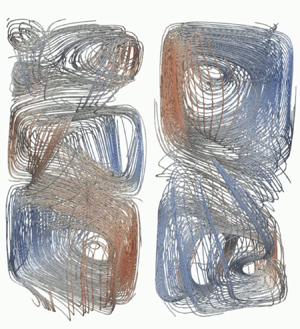
Figure 3. Time-averaged velocity fields in the convection cell (left,  $y$–
$y$– $z$ plane; middle, 3-D velocity field; right, 3-D streamlines) at (a) ${Ra} = 9.33 \times 10^6$, (b) ${Ra} = 5.31 \times 10^7$, (c) ${Ra} = 6.02 \times 10^8$ (the vector length reflects the magnitude of the velocity, the colours represent the amplitude of the vertical velocity component).
Figure 3 shows a significant increase in flow velocity with increasing  $Ra$. We find a prominent torus-shaped flow structure also at ${Ra} = 5.31\times 10^7$ (see figure 3b). However, there is a tendency, especially in the $y$–
$y$– $z$ plane, for two diagonally opposite vortices to intensify and form increasingly close streamlines over the entire height of the convection cell. This resembles the pattern of the large elliptical convection roll with two counter-rotating rolls in the diagonally opposite corners reported by Sun et al. (Reference Sun, Xi and Xia2005a) for instantaneous flow structures and for time-averaged structures in a tilted cell. Likewise, the situation at ${Ra} = 6.02 \times 10^8$ (figure 3c) shows two pairs of rolls. However, the flow pattern seemingly loses symmetry. Four rolls can be identified, with one upper and one lower roll clearly dominating the flow pattern in terms of intensity. This results in a structure that appears more like a DRS with two secondary vortices. The vortex positions are slightly shifted against each other, in particular the centres of the rolls on the right side are much closer to the sidewall.
The observed differences for the various Rayleigh numbers raise the question of whether the increasing turbulence associated with the increase in  $Ra$ could be responsible for the apparent symmetry breaking or whether this is related to slight inaccuracies in the experimental set-up, with the latter never being completely avoidable in practice. The evaluation of the data for ${Ra} = 6.02 \times 10^8$ in figure 4 shows that all angular orientations of the LSC plane can be observed with considerable regularity, but nevertheless a slight deviation from a uniform distribution is found, possibly indicating a slight misalignment of the axis of the convection cell with respect to the gravity vector. Paolillo et al. (Reference Paolillo, Greco, Astarita and Cardone2021) pointed out that asymmetries in the time-averaged flow field could also be due to the chaotic nature of turbulent motion and in such cases the duration of the experiments was not sufficient to obtain symmetric patterns. These initial results presented here from the analysis of our measurements suggest that we may be facing a multi-roll structure, with the number, size and position of the rolls subject to dynamic changes. In the measurements presented here, insufficiently long averaging times could indeed be a problem, but this should actually be most apparent at small $Ra$, since the same measurement times were chosen and the characteristic time scales become distinctly shorter as $Ra$ increases. Vertical profiles of the horizontal velocity averaged across the horizontal section planes of the cylindrical convection cell are drawn in figure 5. As expected, the highest velocities occur near the top and bottom plates. Here, the values exceed the mean value of the horizontal velocity in the entire volume by approximately two and a half times. The horizontal flow in the central area is clearly less intense but by no means negligible.

Figure 4. Time-averaged probability density function (p.d.f.) of the LSC orientation obtained from the temperature measurements at the three rings at  ${Ra} = 6.02 \times 10^8$ using (2.1).

Figure 5. Vertical profiles of the horizontal velocity in the convection cell normalized by their overall mean.
5. Identification of the POD modes in turbulent liquid-metal convection
Paolillo et al. (Reference Paolillo, Greco, Astarita and Cardone2021) presented characteristic POD modes of turbulent convection for  ${Ra} = 1.86 \times 10^8$ and $Pr = 7.6$. They reported that the low-order POD modes can be associated with the manifestation of the LSC in a single-roll state (SRS, modes 1 and 2) and a double-roll state (DRS, modes 3 and 4), respectively. An interesting feature is the pairing of the energy levels which concerns the first six modes. That means that the respective mode pairs represent the same flow structure, differing from each other only by an axial rotation of 90 $^\circ$.
Figure 6 displays the flow morphology for the first eight POD modes obtained from our experiment at a Rayleigh number of  ${Ra} = 6.02 \times 10^8$. The Rayleigh number is approximately a factor of three higher than that of Paolillo et al. (Reference Paolillo, Greco, Astarita and Cardone2021), but the Reynolds number in our liquid-metal convection is supposed to exceed that of Paollilo's water experiment by more than one order of magnitude. As far as the first four modes are concerned, this shows a very good agreement between both experimental configurations. In modes 1 and 2, a clear SRS can be seen, modes 3 and 4 attribute to a DRS, while a TRS becomes obvious in the modes 5 and 6. The latter then do point out a distinct difference, as Paolillo et al. (Reference Paolillo, Greco, Astarita and Cardone2021) observed in modes 5 and 6 the occurrence of four adjacent and alternating up- and downflows, a structure that fits quite well with the occurrence of the second Fourier mode for their azimuthal temperature profiles at the sidewalls, which indicate two minima and maxima of the temperature, respectively. Modes 7 and 8 are characterized by torus-shaped flow structures, which have certain similarities with a DRS or a TRS, respectively. Vertical upflows and downflows still appear on the sidewall, but the recirculation closes in the central region around the cylinder axis.

Figure 6. First eight POD modes for  ${Ra} = 6.02 \times 10^8$: 3-D isosurfaces of the vertical velocity referred to a value corresponding to $\pm$0.1 of the respective maximum value.
Corresponding results for the Rayleigh number of  ${Ra} = 5.31 \times 10^7$ are shown in figure 7. The first mode is clearly assigned to the SRS, but unlike the case of the higher $Ra$, the second mode does not manifest a complement pattern that results from a simple rotation of the first mode. Mode 2 is similar to the SRS, but the structures appear twisted, which already indicates a transition to or a blending with the DRS. The third mode represents the symmetric DRS, while the fourth mode has a structure similar to that of the second mode. The flow patterns of mode 2 and mode 4 can be transformed into each other by mirroring at the $x$–
$x$– $y$ plane followed by a 180 $^\circ$ rotation around the cylinder axis. A TRS appears as a new pattern in the fifth mode, whereby a certain torsion can be seen here as well. The flow structures in modes 6, 7 and 8 resemble slightly twisted DRS and TRS. However, torus-shaped flow components also appear in these modes. From the comparison with the corresponding results at ${Ra} = 6.02 \times 10^8$, we observe the tendency that an increase of $Ra$ appears to stabilize the coherent flow structures of a SRS. This is in agreement with previous findings reported in the literature (Xi & Xia Reference Xi and Xia2008; Weiss & Ahlers Reference Weiss and Ahlers2011).

Figure 7. First eight POD modes for  ${Ra} = 5.31 \times 10^7$: 3-D isosurfaces of the vertical velocity referred to a value corresponding to $\pm$0.1 of the respective maximum value.
Looking at the results for the smaller Rayleigh number of  ${Ra} = 9.33\times 10^6$ in figure 8 confirms this trend. Here, only the first mode can be assigned to the SRS, while mode 2 already represents a DRS. Mode 3 again resembles an SRS, but the structure is somewhat twisted and a disturbance in the form of a torus-shaped roll can be observed on the lid. In addition to mode 2, the appearance of a DRS also dominates modes 4, 5 and 8, while modes 6 and 7 can be assigned to a TRS. However, the basic DRS and TRS patterns do not occur in an unperturbed form in these higher modes. Superpositions with helical and toroidal structures can be noticed.

Figure 8. First eight POD modes for  ${Ra} = 9.33 \times 10^6$: 3-D isosurfaces of the vertical velocity referred to a value corresponding to $\pm$0.1 of the respective maximum value.
Figure 9 shows the energy fraction of a total of the first 42 individual POD modes we were able to identify from the measured data. We observe a drop in the energy spectrum after mode 42, which is most likely due to the limited spatial resolution of the CIFT method. However, since we see that already the energy fractions of the higher modes above mode 15 remain at a nearly constant low energy level far below 1 %, we can assume that the modes beyond mode 40 are not relevant for the reconstruction of the large-scale structures. It is primarily the first eight modes that contribute with a significant amount of energy greater than 1 %. We do not observe a clear pairing of the energy levels for the first six modes as reported by Paolillo et al. (Reference Paolillo, Greco, Astarita and Cardone2021). Only the energy contributions of modes 1 and 2 at  ${Ra} = 6.02 \times 10^8$ are relatively close to each other (at about 22 %), while the share of mode 1 at the smaller $Ra$ is almost one third and mode 2 only reaches values of approximately 15 %. Given that modes 1 and 2 at ${Ra} = 6.02 \times 10^8$ represent the SRS, while at the other $Ra$ only mode 1 can be assigned to an SRS in a clear way, we observe some enhancement of the SRS with increasing $Ra$. While the SRS reaches an energy contribution of approximately 32 % at both ${Ra} = 9.33 \times 10^6$ and ${Ra} = 5.31 \times 10^7$, it accounts for approximately 45 % of the energy at ${Ra}= 6.02 \times 10^8$. Here, modes 3 and 4 present a clear DRS, and their energy contribution can be estimated at approximately 30 %.

Figure 9. The POD spectrum of the velocity field: energy contributions of the first 42 modes at  ${Ra} = 9.33 \times 10^6$, ${Ra} = 5.31 \times 10^7$ and ${Ra} = 6.02 \times 10^8$.
In a next step, we consider the statistical abundance of the energy contributions of the main modes (SRS, DRS and TRS) appearing during the respective measurements to further refine this first rough estimate. For this purpose, the individual POD modes for the various Rayleigh numbers are summarized as follows.
(i) ${Ra}= 9.33 \times 10^6$: SRS (POD modes 1 and 3), DRS (POD modes 2, 4 and 5), TRS (POD modes 6, 7 and 8);
(ii)
${Ra}= 5.31 \times 10^7$: SRS (POD mode 1), DRS (POD modes 2, 3, 4 and 7), TRS (POD modes 5, 6 and 8);(iii)
${Ra}= 6.02 \times 10^8$: SRS (POD modes 1 and 2), DRS (POD modes 3 and 4), TRS (POD modes 5 and 6).


We are aware that this approach can only be an approximation, as the allocation of the respective POD modes made is not unambiguous in all cases. The results in terms of the cumulative probability distributions are shown in figure 10. The values of the energy are scaled by the corresponding maximum value detected within the total duration of a measurement. The progression of the curves in figure 10(a) proves that the POD modes assigned to the SRS tend to provide higher energy contributions, the larger  $Ra$ is. The opposite situation is observed for the DRS (see figure 10b). Also the TRS provides smaller shares of energy for the highest $Ra$ (see figure 10c). Thus, the results presented so far suggest that increasing $Ra$ appears to stabilize SRS at the expense of DRS or TRS. We will elaborate on this point further in § 6.4 when we discuss the reconstruction of instantaneous flow structures.

Figure 10. Cumulative probability distributions (c.d.f.s) of the energy contribution of the main flow structures: (a) SRS ( ${Ra}= 9.33 \times 10^6$, POD modes 1 and 3; ${Ra}= 5.31 \times 10^7$, POD mode 1; ${Ra}= 6.02 \times 10^8$, POD modes 1 and 2), (b) DRS ( ${Ra}= 9.33 \times 10^6$, POD modes 2, 4 and 5; ${Ra}= 5.31 \times 10^7$, POD modes 2, 3, 4 and 7; ${Ra}= 6.02 \times 10^8$, POD modes 3 and 4), (c) TRS ( ${Ra}= 9.33 \times 10^6$, POD modes 6, 7 and 8; ${Ra}= 5.31 \times 10^7$, POD modes 5, 6 and 8; ${Ra}= 6.02 \times 10^8$, POD modes 5 and 6).
6. Temporal dynamics of the large-scale flow structures
After analysing the time-averaged structures and the most relevant POD modes, the interest will now be directed to the temporal behaviour of the flow. It has already been observed that the flow in a convection cell with an aspect ratio of  $\varGamma = 0.5$ behaves in a much more volatile manner than with $\varGamma = 1$ for the same $Ra$ and $Pr$ (Xi & Xia Reference Xi and Xia2008; Stevens, Clercx & Lohse Reference Stevens, Clercx and Lohse2011; Weiss & Ahlers Reference Weiss and Ahlers2011; Paolillo et al. Reference Paolillo, Greco, Astarita and Cardone2021). On the other hand, Ahlers et al. (Reference Ahlers, Bodenschatz, Funfschilling and Hogg2009a) reported a rather stable LSC in the form of a coherent single convection roll for $Pr = 0.674$ and ${Ra} \leq 1.5 \times 10^{11}$. This structure can collapse at irregular time intervals, where the duration of these cessations appear significantly longer than in $\varGamma = 1$ experiments for $Pr = 4.38$ (Brown et al. Reference Brown, Nikolaenko and Ahlers2005a) or in $\varGamma = 0.5$ and $Pr = 5$ (Xi & Xia Reference Xi and Xia2008). Using the same convection cell and fluid as in our present study, Schindler et al. (Reference Schindler, Eckert, Zürner, Schumacher and Vogt2022) suggested a collapse of coherent large-scale flow. This observation shall now be verified in the following sections by analysing the dynamics of the 3-D flow.
6.1. Reynolds number
The Reynolds number  $Re ({Ra}, Pr)$ quantifies the system response with respect to the turbulent momentum transport. Therefore, the primary interest of many investigations so far has been the quantification of the corresponding scaling laws $Re \thicksim {Ra}^{\gamma }$. Data for the turbulent liquid-metal convection in cylinders with $\varGamma = 0.5$ and 1 can be found in Schindler et al. (Reference Schindler, Eckert, Zürner, Schumacher and Vogt2022) and Zürner et al. (Reference Zürner, Schindler, Vogt, Eckert and Schumacher2019), respectively. In the following considerations, we focus on the temporal variations of $Re$ during the experiments and investigate whether there is a relationship between the instantaneous values of $Re$ and the flow structures occurring simultaneously.
The governing flow structure in turbulent convection is a coherent large-scale flow (LSC), which is apparently driven by the detaching plumes. It contains the major part of the kinetic energy of the flow and stands out from the background of turbulent motion. Since a highly turbulent and more complex flow structure develops in a convection cell with aspect ratio 0.5 at high  $Ra$, the question arises whether the flow dynamics can still be quantitatively described by a uniquely defined Reynolds number. In addition, the experimental determination of a characteristic Reynolds number for the entire fluid volume, $Re_{vol}$ involves specific difficulties (especially in liquid metals), since by means of the measuring methods applied so far the flow velocity is determined only indirectly or the measuring domain is usually limited to single positions or specific subregions of the convection cell. Different characteristic velocities can be used for the calculation of $Re$. A first reasonable approach is to base the definition of $Re$ on quantities that can be directly derived from the LSC, which is assumed to be a large convection roll characterized by a typical turnover time $t_{to}$. Using the path length of the circulation as relevant length scale $L$, a characteristic Reynolds number for the LSC can be defined:
 \begin{equation} Re_{LSC} = \frac{L^2}{\nu t_{to}}. \end{equation}
 Earlier studies (see for example, Heslot, Castaign & Libchaber Reference Heslot, Castaign and Libchaber1987; Takeshita et al. Reference Takeshita, Segawa, Glazier and Sano1996; Cioni et al. Reference Cioni, Ciliberto and Sommeria1997) estimated the mean velocity of the global circulation,  $U_{LSC} = L / t_{to}$, from the dominating frequency in the temperature signals under the assumption that the corresponding oscillations arise from perturbations transported by the LSC. Later investigations could assign azimuthal torsional and sloshing modes to this frequency being characteristic for turbulent convection in cylindrical geometries (Funfschilling & Ahlers Reference Funfschilling and Ahlers2004; Funfschilling et al. Reference Funfschilling, Brown and Ahlers2008; Brown & Ahlers Reference Brown and Ahlers2009). Unfortunately, this method is not applicable for our experimental data because in all measurements no dominant oscillation frequencies could be found in either the temperature or velocity signals. This might be a first hint that we are not dealing here with an LSC that has an intact and coherent structure across the entire cell height.
Another approach to determine a characteristic LSC velocity is based on the correlation of temperature signals recorded at various measurement positions (Castaing et al. Reference Castaing, Gunaratne, Heslot, Kadanoff, Libchaber, Thomae, Wu, Zaleski and Zanetti1989; Sano et al. Reference Sano, Wu and Libchaber1989; Takeshita et al. Reference Takeshita, Segawa, Glazier and Sano1996; Chavanne et al. Reference Chavanne, Chilla, Castaing, Hebral, Chabaud and Chaussy1997; Niemela et al. Reference Niemela, Skrbek, Sreenivasan and Donnely2001). Temporary deviations from the temperature occurring successively at two measurement locations are caused by plumes moving across the measurement points. For example, Ahlers, Brown & Nikolaenko (Reference Ahlers, Brown and Nikolaenko2006) extracted the half-turnover time (and finally  $Re_{LSC}$) from the peaks of the cross-correlation functions between temperature signals recorded at opposite azimuthal locations. However, such an approach requires a coherent LSC with predictable topology and streamlines. The recent results by Schindler et al. (Reference Schindler, Eckert, Zürner, Schumacher and Vogt2022) already gave a clear indication that such flow conditions are unlikely to exist in the parameter range studied here. In our convection cell, 16 thermocouples are installed on each of three levels on the sidewall. We have randomly calculated the correlation functions of thermocouples located one above the other in the three planes and of azimuthally opposite thermocouples in the centre plane. It turned out that the correlations between the lower and upper levels as well as the azimuthally opposite positions usually do not result in easily evaluable Gaussian peaks (not shown here). Such Gaussian peaks, from which velocities can be derived, appear in the correlation functions between the centre plane and the upper or lower plane. However, these velocity values differ to a considerable extent. This apparent failure of the method in the case of turbulent liquid-metal convection at aspect ratio $\varGamma = 0.5$ can perhaps be attributed to two causes: (i) the structure of the LSC is disturbed in a way that stable correlation relationships are not established over long distances, (ii) the large thermal diffusivity of the liquid metal leads to a rapid decay of temperature gradients. The results of the flow analysis presented below, will demonstrate that the LSC is subject to extreme variations within a few free-fall times. In addition, the structures are highly twisted, with angle and direction also changing over time. Against this background, it is quite understandable that no stable correlations can be obtained from the experimental temperature data. These difficulties emphasize the importance of direct velocity measurements in liquid metals, which is in the focus of this study.
Zürner et al. (Reference Zürner, Schindler, Vogt, Eckert and Schumacher2019) employed an arrangement of multiple ultrasonic velocity probes and compared three different  $Re$ definitions based on the measurements of the typical horizontal velocity near the plates, the vertical velocity along the sidewall and the turbulent velocity fluctuations in the centre of the convection cell. Their results demonstrate that, as expected, the different $Re$ vary with respect to their absolute values, but the scaling exponent of $Re({Ra})$ is relatively insensitive to the different characteristic velocities. Moreover, the scaling exponent matches very well with DNS results presented by Scheel & Schumacher (Reference Scheel and Schumacher2017).
The CIFT technique provides access to the entire velocity field throughout the convection cell. On this basis we calculate the Reynolds number for the entire volume of the convection cell,  $Re_{vol}$, which takes into account all three velocity components, and compare it with local values of $Re_k$ obtained from the horizontal velocities in three horizontal planes ( $k = bot$, mid, top) at the mid-height of the convection cell or near the two plates. Corresponding results are shown in the figures 25 and 26 in Appendix B.
Figure 11 shows time series of  $Re_{vol}$ recorded for three data sets of various Rayleigh numbers. The data in figure 11 cover a period of 30 000 seconds each, with the full temperature gradient applied approximately one hour after the start of the recordings (3600 s) and switched off 7 hours later (25 200 s). Approximately one hour after applying the temperature gradient, the experiment reaches a quasi-steady state. This concerns mainly the thermal conditions, while $Re_{vol}$ shows persistent strong and irregular fluctuations within the whole measurement period, which seem to increase with increasing $Ra$. Further, in figure 12, time sections from the same data sets are presented, with instantaneous values of $Re_{vol}$ normalized to the respective time-averaged mean values and the time axis normalized to the free-fall time $t_{f\!f}$ and turnover time $t_{to}$, respectively. The definition of the free-fall time is $t_{f\!f} = H^2 / \sqrt {\nu \kappa {Ra}}$. For the calculation of the turnover time, a single-roll LSC with elliptical streamlines was assumed to fill the entire cylinder. As a realistic measure of the mean velocity of the LSC, we chose the time-averaged horizontal component of the velocity field near the plates and extracted it accordingly from the CIFT data. Figure 12 demonstrates that significant changes of the flow state obviously occur occasionally within a few free-fall time units or less than one turnover of a single-roll LSC. In light of the volatility of the flow in the $\varGamma = 0.5$ cell, it is questionable to what extent the choice of turnover time as characteristic time scale is reasonable here. From the analysis of the energy contributions of the main POD modes in the previous section, the existence of a single-roll LSC can be deduced for all three $Ra$ with a tendency of the SRS to strengthen with increasing $Ra$. However, the use of $t_{to}$ only makes sense if the stability of the SRS is guaranteed at least during this time scale, about which the rapid changes of $Re$ in figure 12(b) raise some doubts. The reconstructions of the 3-D flow structures that we present in § 6.4 will confirm the rapid changes in the flow structure and also show that the shape and size of the SRS is also subject to significant changes even during its lifetime. The dramatic changes in LSC velocity and path length, $L$, imply a high degree of uncertainty in the determination of $t_{to}$. Therefore, in the further course of the paper the free-fall time $t_{f\!f}$ is used as the characteristic time scale.

Figure 11. Time series of  $Re$ recorded for three different $Ra$.
$Ra$.

Figure 12. Time series of  $Re_{vol}$ normalized with the time average $\langle Re_{vol} \rangle$, where the time axis is normalized with (a) the free-fall time scale, and (b) the turnover time scale.
Two striking observations from figure 12 are to be noted for all three  $Ra$: (i) with respect to the time average, the temporal fluctuations are of the same order of magnitude regardless of the Rayleigh number, reaching quite impressive values of $\pm 50\,\%$; (ii) these fluctuations often occur on very short time scales (less than 10 free-fall times or one turnover time).
Thus, our measurements at small  $Pr$ confirm previous observations that the change from a $\varGamma = 1$ cell to smaller aspect ratios destabilizes the SRS–LSC, deteriorates the coherence of the large-scale structures and leads to a much more dynamic behaviour of the flow that apparently results from frequent transitions between different roll states (Xi & Xia Reference Xi and Xia2007, Reference Xi and Xia2008; Weiss & Ahlers Reference Weiss and Ahlers2011; Xi et al. Reference Xi, Zhang, Hao and Xia2016; Zwirner et al. Reference Zwirner, Tilgner and Shishkina2020; Schindler et al. Reference Schindler, Eckert, Zürner, Schumacher and Vogt2022). Numerical simulations by Zwirner et al. (Reference Zwirner, Tilgner and Shishkina2020) in a $\varGamma = 0.2$ cylinder for ${Ra} = 5 \times 10^6$ and $Pr = 0.1$ show significant fluctuations of ${Nu}$ and $Re$ occurring within a few free-fall times. While the changes in the Nusselt number reach values of approximately 30 %, the corresponding $Re$ varies less. We assume that the stronger fluctuations of $Re$ by more than 50 % of the mean that we observe are due to the larger $Ra$ and the smaller $Pr$ in our experiment.
6.2. Characterization of the LSC structure from the temperature measurements at the sidewall
A proved method for an assessment of the LSC structure and its dynamics is the identification of the positions of the warm upflows and the cold downflows along the sidewall on the basis of temperature measurements in the sidewall (Xi & Xia Reference Xi and Xia2008; Brown & Ahlers Reference Brown and Ahlers2009; Weiss & Ahlers Reference Weiss and Ahlers2011). If one can assume that the volume of the convection cell is pervaded by large-scale coherent structures moving primarily along the sidewall, conclusions can be drawn with respect to the underlying flow structure. We also followed this approach and performed temperature measurements within three ring-shaped arrays of 16 thermocouples each on the sidewall. For further considerations, including the results and corresponding analysis to be presented in the following sections, we arbitrarily select two time intervals of 200 free-fall times each for the Rayleigh numbers  ${Ra} = 5.31\times 10^7$ and ${Ra} = 6.02\times 10^8$ corresponding to physical time periods of approximately 5800 s and 1750 s, respectively. Figure 13 displays the corresponding space–time plots of the azimuthal temperature distributions at the three rings at $z = H/4$, $H/2$ and $3H/4$ representing the time intervals chosen for ${Ra} = 5.31 \times 10^7$ and ${Ra} = 6.02 \times 10^8$, respectively. These space–time structures result from an interpolation using the measured data of the 16 sensors at each of the three different heights. The red areas indicate an elevation from the mean temperature at that height, which can be associated with plumes rising from the heated bottom, while the blue areas are related to regions of cold fluid sinking downward. As suggested in previous studies, the azimuthal temperature profiles are fitted to a cosine function (see § 2.2) and the line connecting the minimum and maximum temperature values over time is interpreted as the orientation of the LSC plane at the given height. It is noticeable that, near the lid of the cell ( $z = 3H/4$), the blue areas look more sharply structured than the red areas (see figure 13a,b). Above the bottom plate ( $z = H/4$), the situation is the opposite. Here, the blue areas appear more blurred (see figure 13e, f). This is caused by a widening of the plumes on their way between the plates, where the rising plumes suffer a loss of heat due to thermal diffusion. As a result, both the buoyancy and velocity decrease. This also applies, with the opposite sign, to the descending plumes. As we will see in the next section, this effect, which is particularly pronounced in liquid metals due to their small $Pr$, can also be clearly verified in the velocity reconstructions.

Figure 13. Time series of the azimuthal temperature distributions measured along the sidewall at  ${Ra} = 5.31 \times 10^7$ (a,c,e) and ${Ra} = 6.02 \times 10^8$ (b,d, f) and different heights at $z = 3/4 H$ (a,b), $z = H/2$ (c,d) and $z = 1/4 H$ (e, f).
Looking first at the situation for  ${Ra} = 5.31 \times 10^7$ (figure 13a,c,e), we note for the period of approximately the first 80 free-fall times that the ascending plumes are encountered predominantly in an azimuthal range between 100 $^{\circ }$ and 300 $^{\circ }$. In line with this, values around 200 $^{\circ }$ are obtained for the LSC orientation in figure 17(a). According to a first rough estimation, the zones of up-flowing and down-flowing fluid appear clearly separated from each other and similar values for alignment of the LSC plane appear for all three heights, which justifies the assumption that, in a first approximation, we might be dealing with a SRS. However, a closer look reveals that, even under this flow condition, there are always smaller time windows in which the azimuthal temperature distribution has multiple extreme values representing higher Fourier modes. An example becomes manifest in figures 13(a,c) and 14(a) for the planes at $z = 3/4H$ and $H/2$ at $t/t_{f\!f} \approx 436$. Moreover, it is evident that the orientation of the LSC is subject to significant temporal fluctuations. The differences between minimum and maximum values are in the range of approximately 120 $^{\circ }$ up to 180 $^{\circ }$, i.e. the variations in orientation almost reach the magnitude of a reversal of flow direction. In addition, strong differences in the orientation at the different heights (up to 160 $^{\circ }$) are observed at the same time. The temporal rates of change in both directions can be estimated from the temperature curves. Notable values up to $40\cdots 50^{\circ } / t_{f\!f}$ are observed which corresponds to approximately $1.5^{\circ }$/s. These estimates are confirmed by looking at the time derivatives of the orientation of the LSC plane in figure 17 (not shown here). In addition, there are significant discrepancies in the orientation in the upper and lower part of the convection cell and in the dynamics of the re-orientation of the LSC plane at the three different heights. At the time $t/t_{f\!f} \approx 476$, the situation changes dramatically. The entire flow structure starts to rotate in the same direction, but after a few free-fall times the direction of motion is opposite in the upper and lower parts of the cylinder. The LSC plane in the upper half completes approximately one full clockwise rotation, while a counterclockwise rotation can be observed in the lower half. In contrast, the temperature signals on the centre plane do not show a clear rotation, but higher Fourier modes are observed at that time (see figure 14b). While the flow structure in the lower part of the cell carries on to rotate almost continuously until the end of the observation window, the initial positions of the up- and downstreaming plumes seem to be almost re-established on the upper and middle measurement planes in time in the range $510 \lesssim t/t_{f\!f} \lesssim 540$, before there are another abrupt changes in the LSC orientation. Further details will be discussed later in connection with figure 17.

Figure 14. Azimuthal temperature distributions measured at  ${Ra} = 5.31 \times 10^7$ at three heights of $z = 1/4 H$ (bot), $z = H/2$ (mid) and $z = 3/4 H$ (top) for (a) $t/t_{f\!f} = 436$, and (b) $t/t_{f\!f} = 476$.
Let us now consider the temperature field within the time interval at  ${Ra} = 6.02 \times 10^8$ (see figure 13b,d, f). As in the case of the smaller $Ra$, we observe similarly strong fluctuations on short time scales of a few free-fall times. These fluctuations are superimposed here by a slow but continuous rotation, with the LSC plane performing a complete 360 $^{\circ }$ rotation over a period of approximately 110 free-fall times (equivalent to approximately 960 s) corresponding to a mean rotation speed of approximately 0.37 $^{\circ }$/s. As in the case with ${Ra} = 5.31\times 10^7$, the upper and lower parts of the flow structure do not always move in the same direction. This is clearly visible in figure 13(b,d, f) for the period $1710 \lesssim t/t_{f\!f} \lesssim 1745$. While the lower part of the fluid rotates almost uniformly clockwise, the upper part rotates one revolution in the opposite direction in this time domain. In a subsequent longer time interval $1745 \lesssim t/t_{f\!f} \lesssim 1815$, the entire structure rotates clockwise. After that ( $1820 \lesssim t/t_{f\!f} \lesssim 1860$), there occur obviously some perturbations of the flow structure in the lower and middle parts of the convection cell. The LSC orientation reveals some jumps before it then seems to continue the rotation in clockwise direction. At approximately the same time, however, the upper part of the flow structure starts moving in the opposite direction. Although the temperature measurements show strong fluctuations, the temperature plots may indicate the existence of a SRS on average within this time period, as clearly demarcated areas for upflows and downflows can be distinguished. However, the assumption, that we are still dealing predominantly with a single-roll LSC here, would indicate an extreme twisting of the LSC plane. We see strong dynamics illustrated by deviations in LSC orientation at the same times at the different heights reaching maximum values of up to 120 $^{\circ }$ (see also next section for further discussion on the LSC orientation). Moreover, these fluctuations appear rather erratic and barely correlated with each other. In addition, we observe the appearance of higher Fourier modes in the azimuthal temperature profiles at many points in time. Thus, it can be hardly excluded that the SRS is undergoing disruptive changes, transitions between different roll states or more complex restructurings. In light of the high dynamics of the structural changes, it is not easy to distinguish between a distinct roll state (SRS or DRS) and less well-defined transition states.
Figure 15 contains examples for azimuthal temperature profiles at the three different heights along the inner sidewall. Here, we have chosen a comparison of two moments ( $t/t_{f\!f} = 1716$ and 1724) in which the global Reynolds number $Re_{vol}$ passes through a minimum and a maximum, respectively. In figure 16 we contrast these temperature data with corresponding reconstructions of the flow field in the $y$–
$y$– $z$ plane made by means of CIFT. At the Reynolds number minimum (figure 16a), a flow structure of four rolls with very low flow intensities is revealed. In the lower part, two rolls are stacked one on top of the other, taking up approximately two thirds of the volume of the convection cell. In the upper third part we recognize two rolls that are slightly offset next to each other. At the moment of the $Re$ maximum (figure 16b), a SRS with smaller corner vortices is observed at the bottom left and at the top right. However, this is not reflected in the same way in the azimuthal temperature profiles in figure 15. Although the flow intensities differ greatly from each other, the differences between the temperature minimum and maximum, $\delta _k$ are of the same order of magnitude in all cases. Surprisingly, the temperature distributions in figure 15(a) could still be used to roughly infer the existence of a SRS, although the flow reconstruction delivers a completely different result. Of course, this comparison is not conclusive, since we only consider the velocity distribution in the $y$–
$y$– $z$ plane in figure 16. However, it should be noted that, even if we do not look specifically at the particular flow structure but at the integral property of the flow intensity in the convection cell, there are some verifiable discrepancies between temperature measurements and the CIFT measurements (see figure 27 in Appendix B). This is a clear indication of the need to analyse the full 3-D reconstructions of the flow field in more detail, which will be done in the following section.

Figure 15. Azimuthal temperature distributions measured at  ${Ra} = 6.02 \times 10^8$ at three heights of $z = 1/4 H$ (bot), $z = H/2$ (mid) and $z = 3/4 H$ (top) for (a) $t/t_{f\!f} = 1716$, and (b) $t/t_{f\!f} = 1724$.

Figure 16. Flow pattern in the  $y$–
$y$– $z$ plane at ${Ra} = 6.02 \times 10^8$: (a) $t/t_{f\!f} = 1716$, and (b) $t/t_{f\!f} = 1724$ (corresponding azimuthal temperature profiles at the sidewall are shown in figure 15).
6.3. Torsional and sloshing mode
The occurrence of torsional oscillations, in which the orientation of the flow at the plates oscillates almost periodically in opposite phase, is an essential feature of a single-roll LSC in a cylinder with aspect ratio 1. Moreover, the flow in aspect ratios  $\varGamma \ge 1$ is characterized by the occurrence of coherent oscillations, whereby this phenomenon is attributed to the torsional and sloshing mode at $\varGamma = 1$ and is associated with the JRV at $\varGamma > 1$. The oscillation periods usually correspond to the turnover of the LSC (Cioni et al. Reference Cioni, Ciliberto and Sommeria1997; Akashi et al. Reference Akashi, Yanagisawa, Tasaka, Vogt, Murai and Eckert2019; Zürner et al. Reference Zürner, Schindler, Vogt, Eckert and Schumacher2019). Thus, it was shown that changes in the orientation of the LSC plane, such as the azimuthal displacement of the horizontal flow direction in the torsional and sloshing modes, move through the convection cell at the characteristic velocity of the LSC (Zürner et al. Reference Zürner, Schindler, Vogt, Eckert and Schumacher2019). The existence of a dominant frequency is then the indicator of a coherent flow structure powered by hot and cold plumes rising and falling in a synchronized manner. So far, we can state, that the large-scale flow in the $\varGamma = 0.5$ cylinder is significantly more volatile compared with $\varGamma = 1$ and that the LSC exists not only as a single-roll pattern, but also occurs as a double- or triple-roll structure. Frequent switching between these roll structures makes the existence of a consistent turnover time questionable. This consideration is apparently supported by our measurements, since a frequency analysis of both the temperature and velocity time series using fast Fourier transformation does not reveal a dominant frequency in the fluctuating signals. Against this background, the question arises whether the torsion mode still exists under these conditions and whether it can be detected in the measured data.
Figure 17 displays the time series of the orientation  $\theta _k$ derived from the temperature measurements within the time windows already applied in the previous sections. As already noticed in § 6.2, there are, on the one hand, time intervals characterized by a relative stability in the sense that the orientation changes moderately, with a similar tendency on all three sensor rings on average. Examples of such time periods, in which a certain integrity of the overall structure is reflected, are the intervals $380 \lesssim t/t_{f\!f} \lesssim 460$ in figure 17(a) and $1750 \lesssim t/t_{f\!f} \lesssim 1810$ in figure 17(b). On the other hand, there are periods in which the orientation changes very rapidly and by a whole turn or more. These rotations often do not affect the entire LSC structure, but may be limited to the upper or lower half of the convection cell. Thus, rapid counter-rotations of upper and lower flow structures manifest themselves e.g. in the intervals $480 \lesssim t/t_{f\!f} \lesssim 490 ({Ra} = 5.31 \times 10^7)$ or $1720 \lesssim t/t_{f\!f} \lesssim 1740 ({Ra} = 6.02 \times 10^8)$. Moreover, two rapid turns in the lower part of the convection cell can be observed for $t/t_{f\!f} \approx 1870$ and 1890 in a short time sequence, without the fluid in the upper part following the same movement. However, even during the moderate periods without striking events there are quite strong fluctuations, which we look at in more detail below.

Figure 17. Time series of the LSC orientation obtained from measurements of the sidewall temperature: (a)  ${Ra} = 5.31 \times 10^7$, (b) ${Ra} = 6.02 \times 10^8$.
Figure 18 shows the LSC orientation for the same time windows as in figure 17 with the values calculated using the CIFT data. The horizontal velocity field was obtained from the 3-D reconstruction by spatial averaging in two horizontal planes with a distance of 27 mm to the respective copper plates and the main flow direction was determined in the centre of the plane. For both experiments a very good agreement with respect to the main dynamics of the orientation angle can be observed between the multi-thermal-probe method and the CIFT approach. However, some specific details, such as the above-mentioned two complete revolutions of the fluid in the lower part of the convection cells, are not confirmed here (compare figures 17b and 18c). The following analysis is based on the CIFT results. In order to obtain a more reliable statement regarding the possible occurrence of the torsion and sloshing modes, we adopted a similar approach as suggested by Weiss & Ahlers (Reference Weiss and Ahlers2011). To distinguish between high-frequency and low-frequency changes in orientation, a matching low-frequency filter was applied to the time series in figures 18(a) and 18(c). The resulting curve containing only the low-frequency fluctuations was subtracted from the original signal. The remaining fluctuations of higher frequencies are presented in figures 18(b) and 18(d). The values of  $\theta _k$ fluctuate around a mean value with amplitudes up to 80 $^{\circ }$, although these fluctuations seem to be somewhat larger for ${Ra} = 5.31 \times 10^7$.

Figure 18. Time series of the LSC orientation obtained from CIFT measurements at a distance of 27 mm from both plates obtained at  ${Ra} = 5.31 \times 10^7$ (a,b) and ${Ra} = 6.02 \times 10^8$ (c,d): (a,c) azimuthal positions of $\theta _{bot}$ and $\theta _{top}$ as a function of time, (b,d) same data as in (a,c), but low-frequency changes (shown as thin red lines) in orientation subtracted.
From figures 18(b) and 18(d), it is difficult to estimate directly whether torsion and sloshing modes are present. Different periods can be found, in which  $\theta _{bot}$ and $\theta _{top}$ seem to oscillate in phase or in antiphase. Therefore, in a next step, we calculate the correlation functions. For these calculations, the result of which can be seen in figure 19, the complete data set covering the entire measuring time was used. In particular, in this point we deviated from the approach of Weiss & Ahlers (Reference Weiss and Ahlers2011), who only considered the time intervals in which the flow is supposed to be dominated by the SRS regime. In the next section, however, we will see that this assignment of well-defined flow states in specified time periods is not so straightforward, at least in the parameter ranges studied here. Nevertheless, the result from figure 19 seems clear, as the cross-correlation functions for both $Ra$ exhibit a negative peak at zero time delay, which, according to Weiss & Ahlers (Reference Weiss and Ahlers2011), can be interpreted as an indication for the existence of a remnant of the torsional and sloshing mode.

Figure 19. Auto-correlation and cross-correlation functions vs delay time  $\tau$.
6.4. Identification of flow modes by means of POD
The POD analysis in § 5 demonstrates that diverse multiple roll structures can occur, with the SRS being the major contributor to the kinetic energy of the large-scale flow. In this section, we will now look at what times and how often which POD modes dominate the convection and how long these flow states typically last. Xi & Xia (Reference Xi and Xia2008) and Weiss & Ahlers (Reference Weiss and Ahlers2011) determined the flow regime using the multi-thermal-probe method. For the existence of SRS or DRS it was claimed that the amplitudes of the cosine fit of the azimuthal temperature profiles,  $\delta _k$, must be above a certain threshold value. Other flow regimes that do not meet this requirement were classified as transitional states (TS). The relationship between the orientations of the LSC plane in the upper and lower parts of the convection cell, $\Delta \theta = \theta _{top}-\theta _{bot}$, decides the assignment as SRS and DRS, assuming that a single roll is associated with largely the same orientation ( $\Delta \theta < 60^{\circ }$), while flows with prevalent opposite orientation ( $\Delta \theta > 120^{\circ }$) imply a DRS. We have demonstrated that we are able to resolve single- and diverse multi-roll structures by means of our CIFT measurements. Thus, we follow the approach of Paolillo et al. (Reference Paolillo, Greco, Astarita and Cardone2021) of identifying the flow regimes by the energy contributions of the POD modes.
The time series of the energy contributions of the first eight POD modes are shown in figure 20 for the selected time windows at  ${Ra} = 5.31 \times 10^7$ and ${Ra} = 6.02 \times 10^8$ together with the volume-averaged Reynolds number $Re_{vol}$. Animations of the 3-D vector field of velocity in the considered time intervals are provided in supplementary movie 1 available at https://doi.org/10.1017/jfm.2023.794 ( ${Ra} = 5.31\times 10^7$) and supplementary movie 2 ( ${Ra} = 6.02\times 10^8$). Individual modes are grouped together according to their basic structures. The same assignments are made here as previously done for figure 10 in § 5. In the case of ${Ra} = 5.31 \times 10^7$, mode 1 represents the SRS, the modes 2, 3, 4 and 7 are related to the DRS, while modes 5, 6 and 8 are considered as contributions to the TRS. For ${Ra} = 6.02 \times 10 ^8$, the modes can be assigned to the main structures in a pairwise manner, where modes 1 and 2 correspond to a SRS, modes 3 and 4 to a DRS and modes 5 and 6 to a TRS. The classification of modes 7 and 8 is not so straightforward. We have summarized these modes in the same way, although they are different toroidal structures of two to four rolls. We will see, however, that the associated energy contribution is very small compared with the other roll structures for the most part.

Figure 20. Time series of the energy contributions of the first eight POD modes to the total kinetic energy of the flow: (a)  ${Ra} = 5.31 \times 10^7$, (b) ${Ra} = 6.02 \times 10^8$.
In both diagrams it is noticeable that the energy inputs of the individual modes fluctuate very strongly on relatively short time scales of a few free-fall times. This corresponds to the behaviour of  $Re_{vol}$. Moreover, it is evident that the positions of the respective maximum values of $Re_{vol}$ coincide quite well with the peaks of the energy contributions of SRS and DRS in particular. Such a high volatility of the flow with frequent changes of the flow modes and accompanied by corresponding fluctuations of ${Nu}$ and $Re$ was also found by Zwirner et al. (Reference Zwirner, Tilgner and Shishkina2020) (see especially figure 1 therein). Their numerical simulations for turbulent convection in a $\varGamma = 0.2$ cylinder at $Pr = 0.1$ reveal nearly synchronous fluctuations of both ${Nu}$ and $Re$, with high values reached together with a SRS or a DRS, and multi-roll structures appearing at times of minimum flow intensity. This tendency is confirmed by our measurements. Within the time intervals of high flow velocities, the first modes, especially the SRS and DRS, dominate. It is interesting to observe that, in the case of ${Ra} = 5.31 \times 10^7$ (figure 20a), the maxima are determined in roughly equal parts by an SRS and DRS, respectively, while at the higher Rayleigh number the SRS appears to be numerically clearly superior (figure 20b). This is also to be expected from the increase of the integral energy portion of the SRS (see figure 9 in § 5). The appearance of a TRS with high energy input occurs extremely rarely, in the data shown here exactly once, in figure 20(b) at $t/t_{f\!f} \thickapprox 1817$.
At this point we make another attempt to estimate the statistical frequency of occurrence and duration of certain flow states from the measured data. For this purpose, the respective data sets are divided into time intervals in which the respective fundamental modes provide the highest energy contribution. Figure 21 presents the probability distributions and the cumulative probability distributions of the lifetime of the main roll regimes in free-fall times units. When the energy fraction of each of the three roll modes was found to be less than 5 % of the time-averaged total kinetic energy, the flow was considered undefined and assigned to a TS. Table 1 contains the time fractions of the modes studied as well as the mean lifetime of the individual states for both  $Ra$. The comparison of both measurements again reveals a strengthening of the significance of the SRS with increasing $Ra$. According to the analysis performed here, the large-scale structures are found to form more frequently a DRS at ${Ra} = 5.31 \times 10^7$ (figure 21a), while at ${Ra} = 6.02 \times 10^8$ the SRS regime reveals a significantly higher occurrence probability (figure 21b). In the case of the smaller Rayleigh number, the SRS is found for approximately one third of the duration of the experiment, while the DRS dominates for more than half of the measurement time. For the higher $Ra$, this is almost reversed. The following is worth noting: as $Ra$ increases, not only does the percentage for SRS increase, but the time shares of TRS and TS also grow at the expense of the DRS. In addition, the average lifetime in free-fall time units increases for all modes. In the case of the smaller Rayleigh number, the lifetimes of SRS and DRS are approximately the same, but when $Ra$ becomes larger, the lifetime of the SRS in units of free-fall time grows more significantly than for the other modes.

Figure 21. Probability distributions (a,b) and c.d.f.s (c,d) of the lifetime of the main roll states at  ${Ra} = 5.31 \times 10^7$ (a,c) and ${Ra} = 6.02 \times 10^8$ (b,d).
Table 1. Time shares and average lifetimes of the main flow modes.

6.5. Reconstruction of instantaneous flow structures
In this section, we will illustrate, by means of some examples, which instantaneous 3-D structures actually exist in the convection cell during the respective time intervals. To this end, we have chosen another time window for  ${Ra} = 6.02 \times 10^8$ in which we find singular peaks of all the major roll regimes SRS, DRS and TRS, as well as an example in which SRS and DRS reach a local maximum simultaneously. The animation of the 3-D vector field of velocity is provided in supplementary movie 3. Figure 22(a) shows the respective time series of the energy contributions of the POD modes and $Re_{vol}$. The mentioned four selected moments are marked at which the snapshots of the 3-D flow structure are visualized.

Figure 22. Snapshots of the 3-D flow pattern at  ${Ra} = 6.02 \times 10^8$. (a) Time series of the energy contributions of the main POD modes and the volume-averaged Reynolds number, (b) streamlines – point A ( $t /t_{f\!f} = 1195$), (c) streamlines – point B ( $t /t_{f\!f} = 1209$), (d) streamlines – point C ( $t /t_{f\!f} = 1233$), (e) streamlines – point D ( $t /t_{f\!f} = 1242$), ( f) vector field - point A, (g) vector field – point B, (h) vector field – point C, (i) vector field – point D. The angular orientation was chosen here so that the structures are best visible. Therefore, deviations from the supplementary movies may occur.
Point A represents one of the short time intervals in which modes 5 and 6 provide the highest energy contribution. The reconstruction of the flow pattern in figure 22(b, f) reveals a TRS accordingly. In this context, it should be noted that flow patterns of three or more rolls exist in all measurements, especially when the Reynolds numbers feature minimum values, while the high- $Re$ periods are dominated by SRS or DRS. A distinct maximum in flow energy is reached in point B of figure 22(a), to which modes 1 and 2 deliver the greatest energy contribution. This flow state follows a DRS of lower intensity at $t / t_{f\!f} = 1201$. With the decay of modes 3 and 4, the energy contribution of modes 1 and 2 starts to grow. The contribution of the DRS regime drops almost to zero initially, but immediately rises again rapidly and reaches a new peak almost simultaneously with the SRS. Transitions from a DRS to an SRS or vice versa have also been examined in previous experiments (Xi & Xia Reference Xi and Xia2008; Weiss & Ahlers Reference Weiss and Ahlers2011; Paolillo et al. Reference Paolillo, Greco, Astarita and Cardone2021). On an appropriate example, that spanned a period of approximately $35 t_{f\!f}$, Paolillo et al. (Reference Paolillo, Greco, Astarita and Cardone2021) likewise reconstructed the behaviour of the POD modes. In their measurement, the initial state is clearly determined by the energy contribution of the DRS. This is followed for approximately $20 t_{f\!f}$ by a transition phase with appreciable contributions of several modes, before the energy contribution of the SRS increases significantly, while all other modes become almost negligible. We find numerous DRS–SRS transitions in our measurements, but they are all often noticeably different in terms of the temporal evolution of the respective energy fractions as well as their 3-D flow patterns. The simultaneous occurrence of the SRS and DRS peaks at point B is reflected in the flow structure in such a way that one recognizes a rather two-roll structure, but in which a significant part of the streamlines are connected over the entire cell height (see figure 22c,g). In the same time window in figure 22(a), however, we also find both an SRS and a DRS peak, in which almost exclusively only modes 1 and 2 (point C) or 3 and 4 (point D) dominate. The corresponding flow structures in the figures 22(d,h) and 22(e,i) show a single-roll and a double-roll LSC. But here too, both structures are not ideally formed. The large circulation of the SRS does not extend over the entire height of the cell and is supplemented by a smaller roll at the bottom, while another corner vortex is also visible at the bottom of the double roll.
Another specific example of the development of a SRS and its transition to a DRS at  ${Ra} = 6.02 \times 10^8$ is shown in figure 23. This observation concerns a smaller section of the time window already presented in figure 20(b). This time we also depict the energy contributions of the POD modes together with the difference of the LSC orientation at the lower and upper rings of the temperature sensors, $\Delta \theta = \theta _{top} - \theta _{bot}$. This quantity is suggested as an indicator to distinguish between SRS and DRS assuming a SRS for $\Delta \theta < 60^{\circ }$ and a DRS for $\Delta \theta > 120^{\circ }$ (Xi & Xia Reference Xi and Xia2008; Weiss & Ahlers Reference Weiss and Ahlers2011). At point E, we start from a state of very low kinetic energy and small flow velocities (see figure 23b). At time F, the flow at both plates has initially intensified perceptibly (figure 23c), and at time G, one can observe the emergence of stronger plumes that noticeably drive the flow in the volume (figure 23d). The energy of the SRS and flow velocities reach a distinct maximum at time H as shown in figure 23(e). On the left side two strong rising and falling plumes can be seen, which, however, converge at an almost identical azimuthal position. As a result, the descending flow is obviously deflected from the sidewall and evades into the centre of the convection cell. The ascending flow appears to continue up the sidewall, but changes its azimuthal position counterclockwise with increasing height. This rearrangement of the flow structure is apparently associated with higher dissipation. As a result, the velocities decrease significantly, particularly in the centre of the cell as can be seen at time I in figure 23( f). However, the flows in both the upper and lower regions of the convection cell reduce only to a certain extent and form a new DRS at time J in figure 23(g).

Figure 23. Snapshots of the entire 3-D vector field and the distribution of the vertical velocity across the horizontal planes at  $z/H = 0.25$, 0.5 and 0.75 for ${Ra} = 6.02 \times 10^8$: (a) time series of the energy contributions of the main POD modes and the difference of the orientation of the horizontal flow near the plates ( $z/H = 0.1$ and 0.9, respectively), (b) point E, (c) point F, (d) point G, (e) point H, ( f) point I, (g) point J, the colours represent the vertical velocity. The angular orientation was chosen here so that the structures are best visible. Therefore, deviations from the supplementary movies may occur.
Figure 23(a) provides the at first glance astonishing finding that the transition from SRS to DRS seems to have hardly any effect on  $\Delta \theta$ in the case at hand, and it also contradicts the impression that can be gained from panels (b–f). At point H, which coincides with the SRS maximum, $\Delta \theta$ shows a value of 47.4 $^{\circ }$, while $\Delta \theta = -58.6^{\circ }$ in the DRS maximum at time J. The corresponding azimuthal temperature profiles recorded for both moments in time at $z = 1/4 H$ and $z = 3/4 H$, respectively, are presented in figure 24. In agreement with the energy contributions of the POD modes in figure 23(a), which reveal a more intense flow for the case of the SRS maximum in point H, figure 24(a) shows correspondingly larger amplitudes of the cosine fit of the temperature distribution compared with the DRS maximum in figure 24(b). In the latter case, however, the positions of minimum and maximum temperatures are no longer so straightforward to determine, and the cosine fit method is obviously also more error prone here. A closer look at the flow structures reveals the following issues:
(i) The regions of ascending or descending flow on the sidewall vary greatly in terms of their location and extent. For example, crescent-shaped velocity distributions are often observed, with the regions of ascending (descending) flow near the bottom (of the lid) leaning against the sidewall over a wide area, while the oppositely directed flow spreads more toward the centre.
(ii) Since the pattern of upflows and downflows is not symmetrical within the horizontal cross-section, the positions of the temperature minimum and maximum are also usually not exactly opposite to each other. This leads to inaccuracies in the application of the cosine function when fitting the azimuthal profiles.
(iii) The structures of both the single-roll and the double-roll circulations are often seriously twisted. Due to the complexity of the flow, an exact discrimination between a seriously twisted single roll and a double-roll state is difficult to obtain. A more detailed analysis is foreseen for future work, when the measurement system will be extended by an additional excitation magnetic field in horizontal direction.


It can also be seen in the vertical velocity distributions in figure 23 that the cross-sectional area of the plume increases significantly with distance from the plate where it has detached. Moreover, the velocity in the plumes successively decreases with increasing distance from their detachment locations. This is obviously due to the high thermal conductivity of the fluid, which causes the superheat of the plumes to spread rather rapidly to the adjacent zones. This observation is in agreement with the qualitative finding of the broadening of the temperature distributions in figure 13. The thermal dissipation of the plumes is supposed to have an influence on the stability and coherence of the LSC (Stringano & Verzicco Reference Stringano and Verzicco2006). The decrease in the temperature difference between the plumes and the surrounding fluid results in a loss of buoyancy of the plumes relative to the surrounding fluid and a corresponding reduction in velocity. A further interesting aspect is that the detaching plumes usually extend over narrow edge regions along the sidewall resulting in crescent-shaped patterns and at certain times tend to fill the central region of the cross-sectional area when arriving at the opposite plate.
7. Summary
The present study reports on an experimental investigation of the 3-D flow structures in turbulent RBC in liquid metals. Liquid metals as fluids with small Prandtl numbers are a very attractive object of investigation since, for the same values of the Rayleigh number, considerably more free-fall times can be recorded in the same time and these flows feature significantly higher degrees of turbulence compared with measurements in water or gases. However, the more complicated handling of liquid metals and the limited availability of suitable measurement techniques appear to be the main reasons that these fluids have been much less studied to date than fluids at higher  $Pr$. For this reason, we have focused here in particular on a comprehensive instrumentation of the flow to measure both temperature and velocity fields to gain insight into the 3-D structure and dynamics of the LSC. Contactless inductive flow tomography used in this study greatly expands the experimenter's toolbox by capturing the entire velocity field throughout the volume during one measurement. In the case of liquid-metal convection, the CIFT technique enables, for the first time, the integral Reynolds number $Re_{vol}$ for the entire volume of the sample to be determined from the experiment. On the one hand, with access to $Re_{vol}$, the options for comparison with corresponding numerical simulations, that can access the entire velocity field, are expanded. On the other hand, the development of the flow in the entire cell can also be contrasted with the local measurements, which directly record the intensity of the LSC by means of a suitably selected sensor arrangement. The CIFT arrangement of a vertical excitation field and an array of 42 magnetic field sensors has proven to be very effective in revealing the 3-D large-scale flow, very robustly and reliably identifying various roll structures and describing their transitions into each other. The number and arrangement of sensors naturally imposes limitations on the size of the identifiable velocity structures. It also needs to be investigated in more detail whether and to what extend the use of a single excitation field in the $z$-direction limits the accuracy of the reconstruction.
In parallel with the flow measurements by means of CIFT, the multi-thermal-probe technique was applied to determine the structure and temporal behaviour of the LSC using temperature measurements on the sidewall. This method has proven to be quite robust and efficient to perform a classification of the flow structures on the cylinder wall. However, in the case of turbulent liquid-metal convection investigated here, this approach reaches its limits when dealing with rapidly changing 3-D flow patterns. Obviously, temperature measurements on the sidewall cannot capture the entire possibility space of 3-D structures. The limitations of the multi-thermal-probe method with respect to flow reconstruction are primarily due to the limited number of sensors and their fixed measurement positions on the sidewall. This results in poor resolution in the vertical direction, while no information is available in the radial direction. Another critical issue is the use of a cosine fit to determine the LSC orientation, since the distance between the centres of upstream and downstream flow is usually not equidistant (Stevens et al. Reference Stevens, Clercx and Lohse2011). It would be interesting to investigate the correlation between temperature and flow measurements in more detail in the future, also in view of the fact that in the case of small  $Pr$ significant deviations between temperature and velocity fields are to be expected, whereby the temperature field should be much smoother. Flow measurements have the obvious advantage that velocities are captured directly. In case of turbulent fully 3-D flows, moreover, the simultaneous acquisition of the flow field in the entire volume is an important aspect of intricate flow structures and their complex dynamics. It becomes evident that a simple interpretation of single features is not always sufficient and can provoke misinterpretations. An example is the probing of the LSC orientation by ultrasound Doppler profiling near the copper plates (Zürner et al. Reference Zürner, Schindler, Vogt, Eckert and Schumacher2019; Schindler et al. Reference Schindler, Eckert, Zürner, Schumacher and Vogt2022). The 2-D vector of the horizontal velocity is calculated at the intersection of two measuring lines and the direction of the flow along the plates is derived. This concept fails if the incoming plume hits the plate in the centre rather than in the edge zone. Moreover, the phenomenon of decoupled rotation in the upper and lower halves of the convection cell, which was observed a few times in our measurements, as well as a strong twisting of the structures, makes it difficult to unambiguously identify the respective roll structure from the flow direction at the plates alone.
The reconstructions of the large-scale flow from the CIFT data reveal a wide variety of flow patterns that can be assigned to single- or multi-roll structures to a first approximation, with the number of rolls, their size, orientation and location changing very dynamically during the entire duration of the experiment. The transitions between different flow regimes occur in periods of a few free-fall times and thus proceed faster than a hypothetical turnover time, which can be calculated from the LSC velocity near the copper plates and the assumption of a coherent LSC filling the entire convection cell. This result, that the respective flow modes can no longer be considered stable even over the period of a turnover time, as well as the fact that neither in the temperature nor in the velocity signals a characteristic coherent frequency can be located, are in our eyes important indications that the flow has essentially lost its coherent properties. A coherent large-scale flow means that even local changes or perturbations move across the entire structure with a defined velocity corresponding to the turnover velocity, and would be detectable at different points with the respective time offset. The LSC is coherent across the entire cell if enduring correlations can be found at the most distant points, i.e. at the opposing plates. We observe in the velocity data that the LSC is no longer well synchronized here, i.e. plumes detach both temporally and spatially in an uncoordinated and irregular manner at the copper plates. As a consequence, it often happens that ascending and descending plumes collide, causing the flow to deflect to the side or into the interior of the cylinder, or even cancel each other out due to enhanced dissipation. This favours the formation of multi-roll structures due to strong horizontal flow components and vortex reconnection. In addition, a trend towards toroidal structures can be observed, especially near the plates.
The question of whether there is a torsional and sloshing mode in the  $\varGamma = 0.5$ cylinder, as in the case of aspect ratio one, cannot be answered so easily. The fact that the fluid motion in the upper and lower parts of the LSC structure appears to be out of synchronization can be taken as an argument that there are no torsional and sloshing modes. This conclusion is supported by the power spectra of the temperature time series recorded by the respective thermocouples which do not reveal any dominating frequency of a well-defined coherent oscillation. On the other hand, however, the analysis of the orientation of the horizontal flow on the opposing plates discloses an anti-correlation relationship as is typical for the torsional and sloshing mode (see figure 19). Torsional vibrations of a coherent structure should result in one dominant frequency, but with several competing structures of different length scales, the spectrum could become more diffuse and spreads over different frequencies.
The POD analysis for a SRS shows the highest energy fraction for all three  $Ra$. Thus, it is understandable that mostly SRS are detected particularly at the moments when the Reynolds number reaches a maximum. However, flow reconstruction using CIFT shows that this does not necessarily mean that an SRS in a kind of pure form as a singular circulation roll dominates the flow in the convection cell. The singular rolls compete with corner vortices, appear for a short time and disappear relatively quickly by splitting into multiple rolls. The POD analysis suggests that the formation of the SRS is favoured with increasing $Ra$. On the basis of the energy fractions of the various POD modes, the SRS is the most abundant flow mode at the highest Rayleigh number investigated here of ${Ra} = 6.02 \times 10^8$, while the DRS occupies the largest time fraction at ${Ra} = 5.31 \times 10^7$. However, the stability of the flow as a whole seems to benefit from a higher $Ra$. This can be concluded from the increase of the mean lifetime of the main POD modes in units of the free-fall time.
The next step in our work program concerns the link between the properties of highly turbulent 3-D flow described in the current paper and the heat transport through the fluid layer. The temperature drop across the convection cell is essentially due to gradients in the thermal boundary layers, while the turbulent flow in the bulk provides mixing and a nearly homogeneous temperature distribution in the volume between the boundary layers. Although it is not entirely clear which parts of the heat transfer are due to the interfaces or the bulk flow, a change in the coherent properties should be reflected in the transport characteristics. Finally, a special feature of fluids with small  $Pr$ comes into play. While the thermal boundary layer is virtually hidden in the viscous boundary layer at high $Pr$, the situation is exactly the opposite in the liquid metal. The thermal boundary layer is much thicker than the viscous boundary layer and thus exposed to the turbulent fluctuations of large-scale motion. The consequences of this situation for heat transport are still largely unknown and will be investigated in forthcoming work.
Supplementary movies
Supplementary movies are available at https://doi.org/10.1017/jfm.2023.794.
Acknowledgements
This work is supported by the Deutsche Forschungsgemeinschaft (DFG) under the grant VO 2331/1.
Funding
We are most grateful to J. Schumacher and T. Zürner for fruitful and stimulating discussions. We would like to thank S. Sonntag and T. Gundrum for their contribution to the construction and implementation of the CIFT measuring apparatus.
Declaration of interests
The authors report no conflict of interest.
Appendix A. General mathematical basis of CIFT
The CIFT technique takes advantage of the fact that the velocity field  $\boldsymbol {u}$ of an electrically conductive fluid with homogeneous electrical conductivity $\sigma$ in the presence of a constant magnetic field $\boldsymbol {B}_0$ generates electric eddy currents $\boldsymbol {j}$ in the same fluid according to Ohm‘s law
 \begin{equation} \boldsymbol{j} = \sigma(\boldsymbol{u}\times\boldsymbol{B}_0-\boldsymbol{\nabla}\phi), \end{equation}
wherein  $\phi$ is the scalar electric potential. These eddy currents $\boldsymbol {j}$, in turn, generate their own flow-induced magnetic field $\boldsymbol {b}$, which is spatially and temporally structured according to the flow field. Thus, $\boldsymbol {b}$ contains essential information from which the global flow field can be reconstructed by solving a linear inverse problem with an appropriate regularization technique. The flow-induced magnetic field $\boldsymbol {b}$ at any location $\boldsymbol {r}$ is calculated by applying Biot-Savart's law to (A1) and solving the emerging Poisson equation for the potential with insulating walls as boundary condition
 \begin{equation} \nabla^2 \phi = \boldsymbol{\nabla}\boldsymbol{\cdot} (\boldsymbol{u}\times\boldsymbol{B}_0). \end{equation}
The resulting integral equation system is valid for low magnetic Reynolds numbers ( $R_m = \mu _0\sigma LU \ll 1$ with $\mu _0, L, U$ denoting the magnetic permeability, characteristic length scale and velocity):
 $$\begin{gather} \boldsymbol{b}(\boldsymbol{r}) = \frac{\sigma\mu_0}{4{\rm \pi}} \left( \iiint_{V}\frac{(\boldsymbol{u}(\boldsymbol{r}^{\prime}) \times\boldsymbol{B}_0(\boldsymbol{r}^{\prime}))\times(\boldsymbol{r}- \boldsymbol{r}^{\prime})} {\mid \boldsymbol{r}-\boldsymbol{r}^{\prime} \mid^3}\, {\rm d} V^{\prime} - \unicode{x222F}_S\phi(\boldsymbol{s}^{\prime}) \frac{\boldsymbol{n}(\boldsymbol{s}^{\prime})\times(\boldsymbol{r}- \boldsymbol{s}^{\prime})}{\mid \boldsymbol{r}-\boldsymbol{s}^{\prime} \mid^3}\, {\rm d} S^{\prime}\right), \end{gather}$$
 $$\begin{gather}\phi(\boldsymbol{s}) = \frac{1}{4{\rm \pi} p(\boldsymbol{s})} \left(\iiint_{V} \frac{(\boldsymbol{u}(\boldsymbol{r}^{\prime})\times\boldsymbol{B}_0 (\boldsymbol{r}^{\prime}))\boldsymbol{\cdot} (\boldsymbol{s}-\boldsymbol{r}^{\prime})} {| \boldsymbol{s}-\boldsymbol{r}^{\prime}|^3}\, {\rm d} V^{\prime} - \unicode{x222F}_S\phi(\boldsymbol{s}^{\prime}) \frac{\boldsymbol{n}(\boldsymbol{s}^{\prime})\boldsymbol{\cdot} (\boldsymbol{s}-\boldsymbol{s}^{\prime})}{| \boldsymbol{s}-\boldsymbol{s}^{\prime} |^3}\, {\rm d} S^{\prime} \right), \end{gather}$$
with  $S = \partial V$ being the boundary of the fluid volume $V$ and $\boldsymbol {n}(\boldsymbol {s})$ the normal vector at the location $\boldsymbol {s}$ on the surface. The factor $p$ is governed by the shape of the boundary surface, depends on the solid angle at the position $\boldsymbol {s}$ and is 0.5 for flat surfaces (Jacobs, Wondrak & Stefani Reference Jacobs, Wondrak and Stefani2018). The integral equations are solved numerically by discretizing $V$ and $S$ with linear shape functions resulting in a linear equation system with respect to the velocity. The discretized velocity field $\tilde {\boldsymbol {u}}$ can be reconstructed by minimizing the following quadratic functional:
 \begin{equation} \min_{\tilde{u}}\left(\sum_j \| {\boldsymbol{\mathsf{M}}}(\boldsymbol{B}_{0,j}) \tilde{\boldsymbol{u}}-\tilde{\boldsymbol{b}}\|_{2}^{2}+\lambda_R\| {\boldsymbol{\mathsf{A}}}\tilde{\boldsymbol{u}}\|_{2}^{2}+\lambda_D\|\boldsymbol{\nabla}\boldsymbol{\cdot} \tilde{\boldsymbol{u}}\|_{2}^{2}\right) , \end{equation}
where  ${\boldsymbol{\mathsf{M}}}(\boldsymbol {B}_{0,j}$) is the linear operator derived from the integral equation system given in (A3) and (A4) for the $j$th applied magnetic field $\boldsymbol {B}_{0,j}$ and $\tilde {\boldsymbol {b}}$ the vector containing the magnetic fields measured at the sensors. The parameter $\lambda _D$ is chosen large to ensure the divergence-free condition of the reconstructed velocity and $\lambda _R$ represents the Tikhonov regularization parameter used to mitigate the intrinsic non-uniqueness of the inverse problem. The matrix ${\boldsymbol{\mathsf{A}}}$ of the Tikhonov regularization weights each velocity component with its representative volume. The best value of $\lambda _R$ is determined by the L-curve method using the real-time reconstruction method described in Wondrak et al. (Reference Wondrak, Galindo, Stefani, Schindler, Vogt and Eckert2020) and Glavinić et al. (Reference Glavinić, Galindo, Stefani, Eckert and Wondrak2022a).
It is important to note that, from a mathematical point of view, two excitation fields in different directions are required for a full 3-D reconstruction of the velocity field with its poloidal and toroidal components (Stefani & Gerbeth Reference Stefani and Gerbeth2000a,Reference Stefani and Gerbethb). However, in our particular case of an elongated cylindrical convection cell the velocity structure is mainly determined by the poloidal flow components along the height of the vessel. Therefore, an excitation magnetic field in axial direction that enables the reconstruction of the poloidal velocity components is basically sufficient. While, under this condition, only the horizontal flow components contribute to the electromotive force  $\boldsymbol {u} \times \boldsymbol {B}_0$, the vertical components are fixed by the divergence-free condition (Wondrak et al. Reference Wondrak, Pal, Stefani, Galindo and Eckert2018, Reference Wondrak, Galindo, Stefani, Schindler, Vogt and Eckert2020). The main features of the flow structure like the number, orientation and size of the convection rolls can, therefore, be reconstructed with a reasonable quality. This is a tenable compromise which allows to reduce the experimental efforts and to gain a high temporal resolution of 1 Hz. The extension of the system to measurements with two excitation magnetic fields is a work in progress.
Appendix B. Dynamics of the flow intensity
A remarkable property of the turbulent liquid metal convection in the  $\varGamma = 0.5$ cylinder considered here is the occurrence of strong temporal fluctuations in flow intensity, which we have already seen in the volume-averaged values of the Reynolds number in § 6.1. Furthermore, it is to be expected that also distinct local differences appear in the velocity field within the convection cell, since the LSC is known to be driven by thermal plumes that form on the plates, detach there and preferentially move along the sidewall towards the opposite plate.
Figure 25 compares time series of  $Re_{vol}$ with those of the Reynolds numbers determined from horizontal velocity fields reconstructed for the horizontal midplane of the cylinder, $Re_{mid}$ and two planes in a distance of 27 mm from both copper plates, $Re_{bot}$ and $Re_{top}$. While the amplitudes of $Re_{vol}$ and $Re_{mid}$ are of the same order of magnitude, substantially higher velocities occur near the plates. In general, this is in agreement with the results of Zürner et al. (Reference Zürner, Schindler, Vogt, Eckert and Schumacher2019) and is understandable since the measurements near the plates capture the region where the circulation closes with a high degree of certainty, regardless of which roll structure dominates; $Re_{bot}$ and $Re_{top}$ reveal strong fluctuations likely associated with the development and detachment of plumes at the plates. However, no regularities can be seen here in the sense that the dynamics of the plumes at the bottom and the top of the cylinder is correlated in any way.

Figure 25. Time series of various Reynolds numbers normalized with the time average  $\langle Re_{vol} \rangle$ and obtained for different regions in the convection cell within a selected time interval recorded at (a) ${Ra} = 5.31 \times 10^7$ and (b) ${Ra} = 6.02 \times 10^8$.
This is confirmed by the cross-correlation presented in figure 26. The correlation between  $Re_{bot}$ and $Re_{top}$ appears to be rather weak, which indicates that the variations in the volume-averaged Reynolds number can be attributed mainly to the fluctuations in the velocities at the plates. It is likely that plume formation and detachment on the plates are the cause of these significant fluctuations in $Re$. In contrast, the horizontal velocity fields on the three levels are only weakly correlated.

Figure 26. Cross-correlation considering various Reynolds numbers obtained at different regions in the convection cell (a)  ${Ra} = 5.31 \times 10^7$ and (b) ${Ra} = 6.02 \times 10^8$.
Figure 27 presents a comparison between the volume-averaged Reynolds numbers and the corresponding amplitudes  $\delta _k$ from the temperature fits (see § 6.2 for the corresponding temperature measurements). Although some maximum peaks appear to coincide, the $Re_{vol}$ values obtained from the CIFT measurements and the temperature data are not perfectly correlated. However, the temperature measurements at the sidewall also reflect the high volatility of the LSC.

Figure 27. Time series of  $Re$ and the amplitudes $\delta _k$ of the temperature fits: (a) ${Ra} = 5.31 \times 10^7$ and (b) ${Ra} = 6.02 \times 10^8$.


 Open access