


1. INTRODUCTION
Winter surface mass balance, or ‘winter balance’, is the net accumulation and ablation of snow over the winter season (Cogley and others, Reference Cogley2011), which constitutes glacier mass input. Winter balance (B w) is half of the seasonally resolved mass balance, initializes summer ablation conditions and must be estimated to simulate energy and mass exchange between the land and atmosphere (e.g. Hock, Reference Hock2005; Réveillet and others, Reference Réveillet, Vincent, Six and Rabatel2016). Effectively representing the spatial distribution of snow on glaciers is also central to monitoring surface run-off and its downstream effects (e.g. Clark and others, Reference Clark2011).
Winter balance is notoriously difficult to estimate (e.g. Dadić and others, Reference Dadić, Mott, Lehning and Burlando2010; Cogley and others, Reference Cogley2011). Snow distribution in alpine regions is highly variable with short correlation length scales (e.g. Anderton and others, Reference Anderton, White and Alvera2004; Egli and others, Reference Egli, Griessinger and Jonas2011; Grünewald and others, Reference Grünewald, Schirmer, Mott and Lehning2010; Helbig and van Herwijnen, Reference Helbig and van Herwijnen2017; López-Moreno and others, Reference López-Moreno, Fassnacht, Beguería and Latron2011, Reference López-Moreno2013; Machguth and others, Reference Machguth, Eisen, Paul and Hoelzle2006; Marshall and others, Reference Marshall2006) and is influenced by dynamic interactions between the atmosphere and complex topography, operating on multiple spatial and temporal scales (e.g. Barry, Reference Barry1992; Liston and Elder, Reference Liston and Elder2006; Clark and others, Reference Clark2011; Scipión and others, Reference Scipión, Mott, Lehning, Schneebeli and Berne2013). Simultaneously extensive, high resolution and accurate snow distribution measurements on glaciers are therefore difficult to acquire (e.g. Cogley and others, Reference Cogley2011; McGrath and others, Reference McGrath2015) and obtaining such measurements is further complicated by the inaccessibility of many glacierized regions during the winter. Use of physically based models to estimate winter balance is computationally intensive and requires detailed meteorological data to drive the models (Dadić and others, Reference Dadić, Mott, Lehning and Burlando2010). As a result, there is significant uncertainty in estimates of winter balance, thus limiting the ability of models to represent current and projected glacier conditions.
Studies that have focused on obtaining detailed estimates of B w have used a wide range of observational techniques, including direct measurement of snow depth and density (e.g. Cullen and others, Reference Cullen2017), lidar or photogrammetry (e.g. Sold and others, Reference Sold2013) and ground-penetrating radar (e.g. Machguth and others, Reference Machguth, Eisen, Paul and Hoelzle2006; Gusmeroli and others, Reference Gusmeroli, Wolken and Arendt2014; McGrath and others, Reference McGrath2015). Spatial coverage of direct measurements is generally limited and often comprises an elevation transect along the glacier centreline (e.g. Kaser and others, Reference Kaser, Fountain and Jansson2003). Measurements are typically interpolated using linear regression on only a few topographic parameters (e.g. MacDougall and Flowers, Reference MacDougall and Flowers2011), with elevation being the most common. Other established techniques include hand contouring (e.g. Tangborn and others, Reference Tangborn, Krimmel and Meier1975), kriging (e.g. Hock and Jensen, Reference Hock and Jensen1999) and attributing measured winter balance values to elevation bands (e.g. Thibert and others, Reference Thibert, Blanc, Vincent and Eckert2008). Physical snow models have been used to estimate spatial patterns of winter balance (e.g. Mott and others, Reference Mott2008; Schuler and others, Reference Schuler2008; Dadić and others, Reference Dadić, Mott, Lehning and Burlando2010), but the availability of the required meteorological data generally prohibits their widespread application. Error analysis is rarely undertaken and few studies have thoroughly investigated uncertainty in spatially distributed estimates of winter balance (e.g. Schuler and others, Reference Schuler2008).
More sophisticated snow-survey designs and statistical models of snow distribution are widely used in the field of snow science. Surveys described in the snow science literature are generally spatially extensive and designed to measure snow depth and density throughout a basin, ensuring that all terrain types are sampled. A wide array of measurement interpolation methods are used, including linear (e.g. López-Moreno and others, Reference López-Moreno, Latron and Lehmann2010) and non-linear regressions (e.g. Molotch and others, Reference Molotch, Colee, Bales and Dozier2005) that include numerous terrain parameters, as well as geospatial interpolation (e.g. Erxleben and others, Reference Erxleben, Elder and Davis2002; Cullen and others, Reference Cullen2017) including various forms of kriging. Different interpolation methods are also combined; for example, regression kriging (see Supplementary Material) adds kriged residuals to a field obtained with linear regression (e.g. Balk and Elder, Reference Balk and Elder2000). Physical snow models such as SnowTran-3D (Liston and Sturm, Reference Liston and Sturm1998), Alpine3D (Lehning and others, Reference Lehning2006) and SnowDrift3D (Schneiderbauer and Prokop, Reference Schneiderbauer and Prokop2011) are widely used, and errors in estimating snow distribution have been examined from theoretical (e.g. Trujillo and Lehning, Reference Trujillo and Lehning2015) and applied perspectives (e.g. Turcan and Loijens, Reference Turcan and Loijens1975; Woo and Marsh, Reference Woo and Marsh1978; Deems and Painter, Reference Deems and Painter2006).
The goals of this study are to (1) critically examine methods of converting direct snow depth and density measurements to distributed estimates of winter balance; and (2) identify sources of uncertainty, evaluate their magnitude and assess their combined contribution to uncertainty in glacier-wide winter balance. We focus on commonly applied, low-complexity methods of measuring and estimating winter balance in the interest of making our results broadly applicable.
2. STUDY SITE
The St. Elias Mountains (Fig. 1a) rise sharply from the Pacific Ocean, creating a significant climatic gradient between coastal maritime conditions, generated by Aleutian–Gulf of Alaska low-pressure systems, and interior continental conditions, driven by the Yukon–Mackenzie high-pressure system (Taylor-Barge, Reference Taylor-Barge1969). The boundary between the two climatic zones is generally aligned with the divide between the Hubbard and Kaskawulsh Glaciers, ~130 km from the coast. Research on snow distribution and glacier mass balance in this area is limited. A series of research programs, including Project ‘Snow Cornice’ and the Icefield Ranges Research Project, were operational in the 1950s and 60s (Wood, Reference Wood1948; Danby and others, Reference Danby, Hik, Slocombe and Williams2003) and in the last 30 years, there have been a few long-term studies on selected alpine glaciers (e.g. Clarke, Reference Clarke2014), as well as several regional studies of glacier mass balance and dynamics (e.g. Arendt and others, Reference Arendt2008; Berthier and others, Reference Berthier, Schiefer, Clarke, Menounos and Rémy2010; Burgess and others, Reference Burgess, Forster and Larsen2013; Waechter and others, Reference Waechter, Copland and Herdes2015).
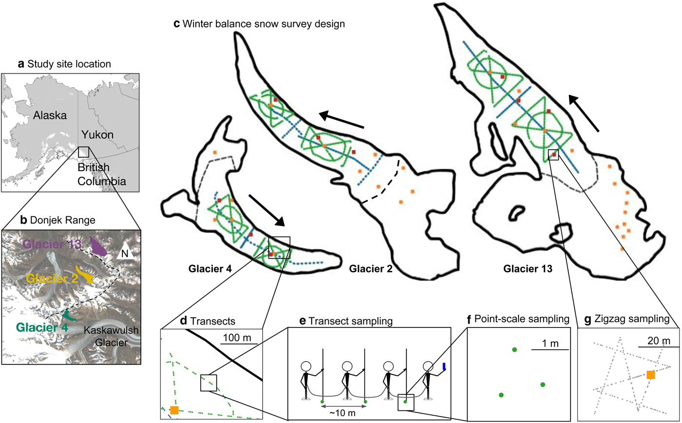
Fig. 1. Study area location and sampling design for Glaciers 4, 2 and 13. (a) Study region in the Donjek Range of the St. Elias Mountains of Yukon, Canada. (b) Study glaciers located along a southwest–northeast transect through the Donjek Range. The local topographic divide is shown as a dashed line. Imagery from Landsat 8 (5 September 2013, data available from the US Geological Survey). (c) Details of the snow-survey sampling design, with centreline and transverse transects (blue dots), hourglass and circle designs (green dots) and locations of snow density measurements (orange squares). Arrows indicate ice-flow directions. Approximate location of ELA on each glacier is shown as a black dashed line. (d) Close up of linear and curvilinear transects. (e) Configuration of navigator and observers. (f) Point-scale snow-depth sampling. (g) Linear-random snow-depth measurements in ‘zigzag’ design (red dots) with one density measurement (orange square) per zigzag.
We carried out winter-balance surveys on three unnamed glaciers in the Donjek Range of the St. Elias Mountains. The Donjek Range is located ~40 km to the east of the regional mountain divide and has an area of ~ 30 × 30 km2. Glacier 4, Glacier 2 and Glacier 13 (labelling adopted from Crompton and Flowers (Reference Crompton and Flowers2016)) are located along a southwest–northeast transect through the range (Fig. 1b, Table 1). These small alpine glaciers are generally oriented southeast–northwest, with Glacier 4 having a predominantly southeast aspect and Glaciers 2 and 13 having generally northwest aspects. The glaciers are situated in valleys with steep walls and have simple geometries. Based on a detailed study of Glacier 2 (Wilson and others, Reference Wilson, Flowers and Mingo2013) and related theoretical modelling (Wilson and Flowers, Reference Wilson and Flowers2013), we suspect all of the study glaciers to be polythermal.
Table 1. Physical characteristics of the study glaciers

3 METHODS
Estimating glacier-wide winter balance (B w) involves transforming measurements of snow depth and density into values of winter balance distributed across a defined grid (b w). We do this in four steps. (1) Obtain direct measurements of snow depth and density in the field. (2) Assign density values to all depth-measurement locations to calculate point-scale values of b w at each location. Winter balance, measured in units of m w.e., can be estimated as the product of snow depth and depth-averaged density. (3) Average all point-scale values of b w within each gridcell of a DEM to obtain the gridcell-averaged b w. (4) Interpolate and extrapolate these gridcell-averaged b w values to obtain estimates of b w in each gridcell across the domain. B w is then calculated by taking the average of all gridcell-averaged b w values for each glacier. For brevity, we refer to these four steps as (1) field measurements, (2) density assignment, (3) gridcell-averaged b w and (4) distributed b w. Detailed methodology for each step is outlined below. We use the SPIRIT SPOT-5 DEM (40 m × 40 m) from 2005 (Korona and others, Reference Korona, Berthier, Bernard, Rémy and Thouvenot2009) throughout this study.
3.1. Field measurements
Our sampling campaign involved four people and occurred between 5 and 15 May 2016, which falls within the period of historical peak snow accumulation in southwestern Yukon (Yukon Snow Survey Bulletin and Water Supply Forecast, 1 May 2016). Snow depth is generally accepted to be more variable than density (Elder and others, Reference Elder, Dozier and Michaelsen1991; Clark and others, Reference Clark2011; López-Moreno and others, Reference López-Moreno2013) so we chose a sampling design that resulted in a high ratio (~55:1) of snow depth to density measurements. In total, we collected more than 9000 snow-depth measurements and more than 100 density measurements throughout the study area (Table 1).
During the field campaign, there were two small accumulation events. The first, on 6 May 2016, also involved high winds so accumulation could not be determined. The second, on 10 May 2016, resulted in 0.01 m w.e. accumulation measured at one location on Glacier 2. Assuming both accumulation events contributed a uniform 0.01 m w.e. accumulation to all study glaciers then our survey did not capture ~3 and ~2% of estimated B w on Glaciers 4 and 2, respectively. We, therefore, assume that these accumulation events were negligible and apply no correction. Positive temperatures and clear skies occurred between 11 and 16 May 2016, which we suspect resulted in melt occurring on Glacier 13. The snow in the lower part of the ablation area of Glacier 13 was isothermal and showed clear signs of melt and metamorphosis. The total amount of melt during the study period was estimated using a degree-day model and found to be small (≤0.01 m w.e., see Supplementary Material) so no corrections were made.
3.1.1. Sampling design
The snow surveys were designed to capture variability in snow depth at regional, basin, gridcell and point scales (Clark and others, Reference Clark2011). To capture variability at the regional scale, we chose three glaciers along a transect aligned with the dominant precipitation gradient (Fig. 1b) (Taylor-Barge, Reference Taylor-Barge1969). To account for basin-scale variability, snow depth was measured along linear and curvilinear transects on each glacier (Fig. 1c) with a sample spacing of 10–60 m (Fig. 1d). Sample spacing was constrained by protocols for safe glacier travel, while survey scope was constrained by the need to complete all surveys within the period of peak accumulation. We selected centreline and transverse transects as the most commonly used survey designs in winter-balance studies (e.g. Kaser and others, Reference Kaser, Fountain and Jansson2003; Machguth and others, Reference Machguth, Eisen, Paul and Hoelzle2006) as well as an hourglass pattern with an inscribed circle, which allows for sampling in multiple directions and easy travel (personal communication from C. Parr, 2016). To capture variability at the grid scale, we densely sampled up to four gridcells on each glacier using a linear-random sampling design (Shea and Jamieson, Reference Shea and Jamieson2010), which we term a ‘zigzag’. To capture point-scale variability, each observer made 3–4 depth measurements within ~1 m (Fig. 1f) at each transect measurement location.
3.1.2. Snow depth: transects
While roped-up for glacier travel with fixed distances between observers, the lead observer used a single-frequency GPS unit (Garmin GPSMAP 64s) to navigate between predefined transect measurement locations (Fig. 1e). The remaining three observers used 3.2 m graduated aluminum avalanche probes to make snow-depth measurements (Kinar and Pomeroy, Reference Kinar and Pomeroy2015). The locations of each set of depth measurements, made by the second, third and fourth observers, are estimated using the recorded location of the first observer, the approximate distance between observers and the direction of travel. The 3–4 point-scale depth measurements are averaged to obtain a single depth measurement at each transect measurement location. When considering variability at the point scale as a source of uncertainty in snow depth measurements, we find that the mean standard deviation of point-scale snow depth measurements is <7% of the mean snow depth for all study glaciers.
Snow-depth sampling was concentrated in the ablation area to ensure that only snow from the current accumulation season was measured. The boundary between snow and firn in the accumulation area can be difficult to detect and often misinterpreted, especially when using an avalanche probe (Grünewald and others, Reference Grünewald, Schirmer, Mott and Lehning2010; Sold and others, Reference Sold2013). We intended to use a firn corer to measure winter balance in the accumulation area, but cold snow combined with positive air temperatures led to cores being unrecoverable. Successful snow-depth measurements within the accumulation area were made either in snow pits or using a Federal Sampler (described below) to unambiguously identify the snow/firn transition.
3.1.3. Snow depth: zigzags
We measured depth at random intervals of 0.3–3.0 m along two ‘Z’-shaped patterns (Shea and Jamieson, Reference Shea and Jamieson2010), resulting in 135–191 measurements per zigzag, within three 40 m × 40 m gridcells (Fig. 1g) per glacier. Random intervals were computer-generated from a uniform distribution in sufficient numbers that each survey was unique. Zigzag locations were randomly chosen within the upper, middle and lower regions of the ablation area of each glacier. Extra time in the field allowed us to measure a fourth zigzag on Glacier 13 in the central ablation area at ~2200 m a.s.l.
3.1.4. Snow density
Snow density was measured using a Snowmetrics wedge cutter in three snow pits (SP) on each glacier. Within the snow pits, we measured a vertical density profile (in 10 cm increments) with the 5 cm × 5 cm × 10 cm wedge-shaped cutter (250 cm3) and a Presola 1000 g spring scale (e.g. Gray and Male, Reference Gray and Male1981; Fierz and others, Reference Fierz2009; Kinar and Pomeroy, Reference Kinar and Pomeroy2015). Wedge-cutter error is ~ ±6% (e.g. Proksch and others, Reference Proksch, Rutter, Fierz and Schneebeli2016; Carroll, Reference Carroll1977). Uncertainty in estimating density from SP measurements also stems from incorrect assignment of density to layers that cannot be sampled (e.g. ice lenses and hard layers). We attempt to quantify this uncertainty by varying estimated ice-layer thickness by ±1 cm (≤100%) of the recorded thickness, ice layer density between 700 and 900 kg m−3 and the density of layers identified as being too hard to sample (but not ice) between 600 and 700 kg m−3. When considering all three sources of uncertainty, the range of integrated density values is always <15% of the reference density. Depth-averaged densities for shallow pits (<50 cm) that contain ice lenses are particularly sensitive to changes in prescribed density and ice-lens thickness.
While snow pits provide the most accurate measure of snow density, digging and sampling a snow pit is time and labour intensive. Therefore, a Geo Scientific Ltd. metric Federal Sampler (FS) (Clyde, Reference Clyde1932) with a 3.2–3.8 cm diameter sampling tube, which directly measures depth-integrated snow water equivalent, was used to augment the SP measurements. A minimum of three FS measurements were taken at each of 7–19 locations on each glacier and an additional eight FS measurements were co-located with two SP profiles for each glacier. Measurements for which the snow core length inside the sampling tube was <90% of the snow depth were discarded. Densities at each measurement location (eight at each SP, three elsewhere) were then averaged, with the standard deviation taken to represent the uncertainty. The mean standard deviation of FS-derived density was ≤4% of the mean density for all glaciers.
3.2. Density assignment
Measured snow density must be interpolated or extrapolated to estimate point-scale b w at each snow-depth sampling location. We employ four commonly used methods to interpolate and extrapolate density (Table 2): (1) calculate mean density over an entire mountain range (e.g. Cullen and others, Reference Cullen2017), (2) calculate mean density for each glacier (e.g. Elder and others, Reference Elder, Dozier and Michaelsen1991; McGrath and others, Reference McGrath2015), (3) linear regression of density on elevation for each glacier (e.g. Elder and others, Reference Elder, Rosenthal and Davis1998; Molotch and others, Reference Molotch, Colee, Bales and Dozier2005) and (4) calculate mean density using inverse-distance weighting (e.g. Molotch and others, Reference Molotch, Colee, Bales and Dozier2005) for each glacier. Densities derived from SP and FS measurements are treated separately, for reasons explained below, resulting in eight possible methods of assigning density.
Table 2. Details of the May 2016 winter-balance survey, including number of snow-depth measurement locations along transects (n T), total length of transects (d T), number of combined snow pit and Federal Sampler density measurement locations (n p), number of zigzag surveys (n zz), number (as percent of total number of gridcells and of the number of gridcells in the ablation area) of gridcells sampled (n s) and the elevation range (as percent of total elevation range and of ablation-area elevation range)

3.3. Gridcell-averaged winter balance
We average one to six (mean of 2.1 measurements) point-scale values of b w within each DEM gridcell to obtain the gridcell-averaged b w. The locations of individual measurements have uncertainty due to the error in the horizontal position given by the GPS unit and the estimation of observer location based on the recorded GPS positions of the navigator. This location uncertainty could result in the incorrect assignment of a point-scale b w measurement to a particular gridcell. However, this source of error is not further investigated because we assume that the uncertainty resulting from incorrect locations of point-scale b w values is captured in the uncertainty derived from zigzag measurements, as described below. Error due to having multiple observers is also evaluated by conducting an analysis of variance (ANOVA) of snow-depth measurements along a transect (amounting to 23 hypothesis tests, one for each transect) and testing for differences between observers. We find no significant differences between snow-depth measurements made by observers along any transect (p > 0.05), with the exception of the first transect on Glacier 4 (51 measurements), where snow-depth measurements collected by one observer were, on average, greater than snow-depth measurements taken by the other two observers (p < 0.01). Since this was the first transect and the only one to show differences by observer, this difference can be considered an anomaly. We conclude that observer bias is not an important effect in this study and therefore apply no observer corrections to the data.
3.4. Distributed winter balance
Gridcell-averaged values of b w are interpolated and extrapolated across each glacier using linear regression (LR) and ordinary kriging (OK). The LR relates gridcell-averaged b w to various topographic parameters. We use this method because it is simple and has precedent for success (e.g. McGrath and others, Reference McGrath2015). Instead of a standard LR, however, we use cross-validation implemented in such a way as to prevent data overfitting, and employ model averaging to allow for all combinations of the chosen topographic parameters. To compliment the LR approach, we also use a Gaussian Process regression with a constant mean and specified covariance, hereafter referred to as OK, to interpolate and extrapolate gridcell-averaged b w. This approach is an interpolation method free of physical interpretation beyond the premise of spatial correlation in the data (e.g. Hock and Jensen, Reference Hock and Jensen1999; Rasmussen and Williams, Reference Rasmussen and Williams2006).
3.4.1. Linear regression
Commonly defined topographic parameters are selected as regressors within the LR. As in McGrath and others (Reference McGrath2015) we include elevation, slope, aspect, curvature, ‘northness’ and a wind-redistribution parameter (Sx from Winstral and others (Reference Winstral, Elder and Davis2002)); we add distance-from-centreline as an additional parameter. Topographic parameters are standardized for use in the LR. The goal of the LR is to obtain a set of fitted regression coefficients (β) that correspond to each topographic parameter (regressor) and to a model intercept. For details on data and methods used to estimate the topographic parameters see the Supplementary Material and Pulwicki (Reference Pulwicki2017). Our sampling design ensured that the ranges of topographic parameters associated with our measurement locations represent more than 70% of the total area of each glacier (except elevation on Glacier 2, where our measurements captured only 50%).
We use a combination of cross-validation and model averaging to avoid overfitting the data, to account for uncertainty in the selected predictors and to maximize the model's predictive ability (Madigan and Raftery, Reference Madigan and Raftery1994; Kohavi, Reference Kohavi1995). Since there are seven predictors, there are 27 possible subsets of predictors, or equivalently, models.
For a given model, we randomly select 1000 subsets of the data (where each subset includes ~2/3 of the data) and fit a multiple LR using least squares (implemented in MATLAB), thus obtaining 1000 sets of β. Distributed b w is then calculated by multiplying the topographic parameters by their corresponding regression coefficients for all DEM gridcells. We use the remaining data (~1/3 of the values) to calculate a RMSE between the estimated and observed b w at the measurement locations. From the 1000 sets of β values, we select the set that results in the lowest RMSE. This set of β has the greatest predictive ability for a particular linear combination of topographic parameters. The procedure above is repeated for each of the models, giving the best β set for each of the 27 models.
With the β's in hand, we move on to prediction of distributed winter balance. To do so, we use Bayesian model averaging. We weight the models according to their relative predictive success, as assessed by the value of the Bayesian Information Criterion (BIC) (Burnham and Anderson, Reference Burnham and Anderson2004). BIC penalizes more complex models, which reduces the risk of overfitting. The final value of each β is then the weighted sum of β from all models. The final estimate of distributed b w is calculated by multiplying the topographic parameters by the final set of β for all DEM gridcells.
3.4.2. Ordinary kriging
Kriging is a method of estimating dependent variables at unsampled locations by using the spatial correlation of measured values to find a set of optimal weights (Davis and Sampson, Reference Davis and Sampson1986; Li and Heap, Reference Li and Heap2008). Kriging assumes spatial correlation between the dependent variables at the sampling locations distributed across a surface and then applies the correlation to interpolate between these locations. Many forms of kriging have been developed to accommodate different data types (e.g. Li and Heap, Reference Li and Heap2008, and sources therein). OK is the simplest form of kriging in cases where the mean of the estimated field is unknown. Unlike LR, OK is neither useful for generating hypotheses to explain the physical controls on snow distribution, nor can it be used to estimate winter balance on unmeasured glaciers. However, we chose to use OK because it does not require external inputs and is, therefore, a means of obtaining B w that is free of physical interpretation beyond the information contained in the covariance matrix.
The OK model can be written y(s) = μ + z(s) + e, where μ is the mean and e is independent white noise with standard deviation σ e (also known as the nugget) that captures the sampling error as well as spatial variation at distances less than those observed in the sampling design (Li and Heap, Reference Li and Heap2008); z(s) follows a mean-zero normal distribution with standard deviation σ z. The covariance of observations at spatial locations s and s′ is written as  $Cov(z(s),\, z(s')) =\sigma ^2_z \, r(s,\,s')$ and r is a specified correlation model. We use the DiceKriging package in R (Roustant and others, Reference Roustant, Ginsbourger and Deville2012) to implement OK. For our application, we employ an isotropic Matérn correlation model with shape parameter ν = 5/2 (see Rasmussen and Williams, Reference Rasmussen and Williams2006). This specification implies a fairly smooth response surface (twice differentiable) and is used in many applications (e.g. Stein, Reference Stein1999). The model parameters, μ, σ e, σ z and range parameter for the Matérn correlation function, are estimated using maximum likelihood. There is no closed form solution for these parameter estimates so they are found numerically. To ensure stability of the maximum likelihood solution, we use 500 random restarts of the DiceKringing package (each with a different initial value of the parameters).
3.5. Uncertainty analysis using a Monte Carlo approach
Three sources of uncertainty are considered separately: the uncertainty due to (1) grid-scale variability of b w (σ GS), (2) the assignment of snow density (σ ρ) and (3) interpolating and extrapolating gridcell-averaged values of b w (σ INT). To quantify the combined uncertainty due to grid-scale variability, the method of density assignment and interpolation uncertainty on estimates of B w, we conduct a Monte Carlo analysis that uses repeated random sampling of input variables to calculate a distribution of output variables (Metropolis and Ulam, Reference Metropolis and Ulam1949). We repeat the random sampling process 1000 times, resulting in a distribution of values of B w based on uncertainties associated with the four steps we implement to derive B w from distributed snow-depth and density measurements. Individual sources of uncertainty are propagated through the conversion of snow depth and density measurements to B w. Finally, the combined effect of all three sources of uncertainty on B w is quantified. We use the standard deviation of the distribution of B w as a useful metric of B w uncertainty. Density assignment uncertainty is calculated as the standard deviation of the eight resulting values of B w. To investigate the spatial patterns in b w uncertainty, we calculate a combined uncertainty, which is equal to the square root of the summed variance of distributed b w that arises from σ GS, σ ρ and σ INT. See Supplementary Material (Figs. S5 and S6) for plots of standard deviation of distributed b w arising from individual sources of uncertainty.
3.5.1. Grid-scale uncertainty (σ GS)
We make use of the zigzag surveys to quantify the true variability of b w at the grid scale. Our limited data do not permit a spatially-resolved assessment of grid-scale uncertainty, so we characterize this uncertainty as uniform across each glacier and represent it by a normal distribution. The distribution is centred at zero and has a standard deviation equal to the mean standard deviation of all zigzag measurements for each glacier. For each iteration of the Monte Carlo, b w values are randomly chosen from the distribution and added to the values of gridcell-averaged b w. These perturbed gridcell-averaged values of b w are then used in the interpolation. We represent uncertainty in B w due to grid-scale uncertainty (σ GS) as the standard deviation of the resulting distribution of B w estimates.
3.5.2. Density assignment uncertainty (σ ρ)
We incorporate uncertainty due to the method of density assignment by carrying forward all eight density interpolation methods (Table 3) when estimating B w. By choosing to retain even the least plausible options, as well as the questionable FS data (see below), this approach results in a generous assessment of uncertainty. We represent the B w uncertainty due to density assignment uncertainty (σ ρ) as the standard deviation of B w estimates calculated using each density assignment method.
3.5.3 Interpolation uncertainty (σ INT)
We represent the uncertainty due to interpolation/extrapolation of gridcell-averaged b w in different ways for LR and OK. LR interpolation uncertainty is represented by a multivariate normal distribution of possible regression coefficients (β). The standard deviation of each distribution is calculated using the covariance of β as outlined in Bagos and Adam (Reference Bagos and Adam2015), which ensures that the β values are internally consistent. The β distributions are randomly sampled and used to calculate gridcell-estimated b w.
OK interpolation uncertainty is represented by the standard deviation for each gridcell-estimated value of b w generated by the DiceKriging package. The standard deviation of B w is then found by taking the square root of the average variance of each gridcell-estimated b w. The final distribution of B w values is centred at the B w estimated with OK. For simplicity, the standard deviation of B w values that results from either LR or OK interpolation/extrapolation uncertainty is referred to as σ INT.
4. RESULTS
4.1. Field measurements
4.1.1. Snow depth
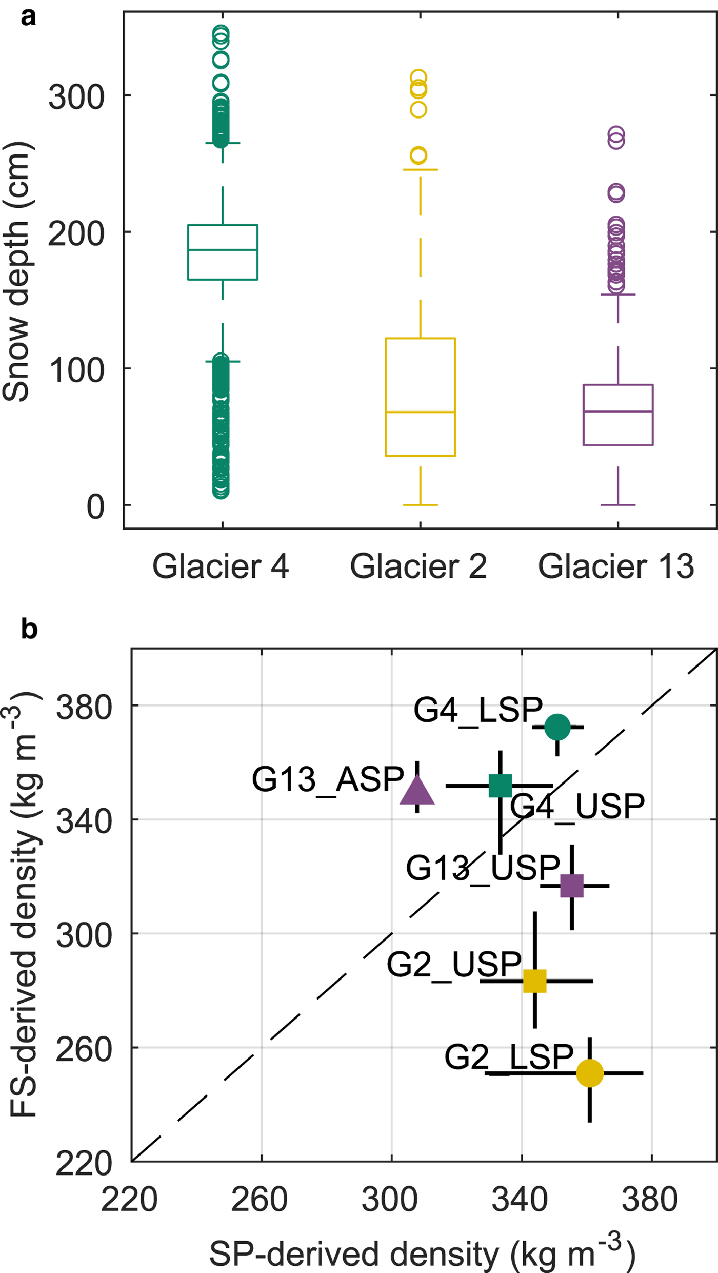
Mean snow depth varied systematically across the study region, with Glacier 4 having the highest mean snow depth and Glacier 13 having the lowest (Fig. 2a). At each measurement location, the median range of measured depths (3–4 points) as a percent of the mean local depth is 2, 11 and 12%, for Glaciers 4, 2 and 13, respectively. While Glacier 4 has the lowest point-scale variability, as assessed above, it also has the highest proportion of outliers, indicating a more variable snow depth across the glacier. The average standard deviation of all zigzag depth measurements is 0.07, 0.17 and 0.14 m, for Glaciers 4, 2 and 13, respectively. When converted to values of b w using the local FS-derived density measurement, the average standard deviation is 0.027 m w.e., 0.035 m w.e. and 0.040 m w.e. Winter-balance data for each zigzag are not normally distributed (Fig. 3).

Fig. 2. Measured snow depth and density. (a) Boxplot of measured snow depth on Glaciers 4, 2 and 13 with the first quartiles (box), median (line within box), minimum and maximum values excluding outliers (bar) and outliers (circles), which are defined as being outside of the range of 1.5 times the quartiles (~± 2.7σ). (b) Comparison of depth-averaged densities estimated using Federal Sampler (FS) measurements and a wedge cutter in a snow pit (SP) for Glacier 4 (G4), Glacier 2 (G2) and Glacier 13 (G13). Labels indicate SP locations in the accumulation area (ASP), upper ablation area (USP) and lower ablation area (LSP). Error bars for SP-derived densities are calculated by varying the thickness and density of layers that are too hard to sample, and error bars for FS-derived densities are the standard deviation of measurements taken at one location. One-to-one line is dashed.

Fig. 3. Distributions of estimated winter-balance values for each zigzag survey in lower (L), middle (M) and upper (U) ablation areas (insets). Local mean has been subtracted. (a) Glacier 4. (b) Glacier 2. (c) Glacier 13.
4.1.2. Snow density
Contrary to expectation, co-located FS and SP measurements are found to be uncorrelated (R 2 = 0.25, Fig. 2b). The FS appears to oversample in deep snow and undersample in shallow snow. Oversampling by small-diameter sampling tubes has been observed in previous studies, with a percent error between 6.8 and 11.8% (e.g. Work and others, Reference Work, Stockwell, Freeman and Beaumont1965; Fames and others, Reference Fames, Peterson, Goodison and Richards1982; Conger and McClung, Reference Conger and DM2009). Studies that use FS often apply a 10% correction to all measurements for this reason (e.g. Molotch and others, Reference Molotch, Colee, Bales and Dozier2005). Oversampling has been attributed to slots ‘shaving’ snow into the tube as it is rotated (e.g. Dixon and Boon, Reference Dixon and Boon2012) and to snow falling into the slots, particularly for snow samples with densities > 400 kg m−3 and snow depths > 1 m (e.g. Beaumont and Work, Reference Beaumont and Work1963). Undersampling is likely to occur due to loss of snow from the bottom of the sampler (Turcan and Loijens, Reference Turcan and Loijens1975). The loss by this mechanism may have occurred in our study, given the isothermal and melt-affected snow conditions observed over the lower reaches of Glaciers 2 and 13. Relatively poor FS spring-scale sensitivity also calls into question the reliability of measurements for snow depths < 20 cm.
Our FS-derived density values are positively correlated with snow depth (R 2 = 0.59). This relationship could be a result of physical processes, such as compaction in deep snow and preferential formation of depth hoar in shallow snow, but is more likely a result of measurement artefacts for a number of reasons. First, the total range of densities measured by the FS seems improbably large (227–431 kg m−3). At the time of sampling, the snowpack had little new snow, few ice lenses and was not saturated; the range of measured densities is, therefore, difficult to explain with physical conditions. Moreover, the range of FS-derived values is much larger than that of SP-derived values when co-located measurements are compared. Second, compaction effects of the magnitude required to explain the density differences between SP and FS measurements would not be expected at the measured snow depths (up to 340 cm). Third, no linear relationship exists between depth and SP-derived density (R 2 = 0.05). These findings suggest that the FS measurements have a bias for which we have not identified a suitable correction. Despite this bias, we use FS-derived densities to generate a range of possible b w estimates and to provide a generous estimate of uncertainty arising from density assignment.
4.2. Density assignment
Given the lack of correlation between co-located SP- and FS-derived densities (Fig. 2), we use the densities derived from these two methods separately (Table 3). SP-derived regional (S1) and glacier-mean (S2) densities are within one standard deviation of the corresponding FS-derived densities (F1 and F2) although SP-derived density values are larger (see Supplementary Material, Table S3). For both SP- and FS-derived densities, the mean density for any given glacier (S2 or F2) is within one standard deviation of the mean across all glaciers (S1 or F1). Correlations between elevation and SP- and FS-derived densities are generally high (R 2 > 0.5) but vary between glaciers (Supplementary Material, Table S3). For any given glacier, the standard deviation of the 3–4 SP- or FS-derived densities is <13% of the mean of those values (S2 or F2) (Supplementary Material, Table S3). We adopt S2 (glacier-wide mean of SP-derived densities) as the reference method of density assignment. Though the method described by S2 does not account for known basin-scale spatial variability in snow density (e.g. Wetlaufer and others, Reference Wetlaufer, Hendrikx and Marshall2016), it is commonly used in winter-balance studies (e.g. Elder and others, Reference Elder, Dozier and Michaelsen1991; McGrath and others, Reference McGrath2015; Cullen and others, Reference Cullen2017).
Table 3. Eight methods used to estimate snow density at unmeasured locations. Source of snow density values include snow pit (SP) and Federal Sampler (FS) measurements. Total number of resulting density values given in parentheses, with n T the total number of snow-depth measurement locations along transects (Table 1)

4.3. Gridcell-averaged winter balance
The distributions of gridcell-averaged b w values for the individual glaciers are similar to those in Fig. 2a but with fewer outliers (see Supplementary Material, Fig. S4). The standard deviations of b w values determined from the zigzag surveys are almost twice as large as the mean standard deviation of point-scale b w values within a gridcell measured along transects (see Supplementary Material, Fig. S5). However, a small number of gridcells sampled in transect surveys have standard deviations in b w that exceed 0.25 m w.e. (~10 times greater than those for zigzag surveys).
4.4. Distributed winter balance
4.4.1. Linear regression
The highest values of estimated b w are found in the upper portions of the accumulation areas of Glaciers 2 and 13 (Fig. 4). These areas also correspond to large values of elevation, slope and wind redistribution. Extrapolation of the positive relationship between b w and elevation, as well as slope and Sx for Glacier 2, results in high b w estimates and large combined uncertainty in these estimates (Fig. 5). On Glacier 4, the distributed b w is nearly uniform (Fig. 4) due to the small regression coefficients for all topographic parameters. The variance explained by the LR-estimated b w differs considerably between glaciers (Fig. 6), with the best correlation between modelled and observed b w occurring for Glacier 2. LR is an especially poor predictor of b w on Glacier 4, where B w can be estimated equally well using the mean of the data. RMSE is also the highest for Glacier 4 (Table 4).
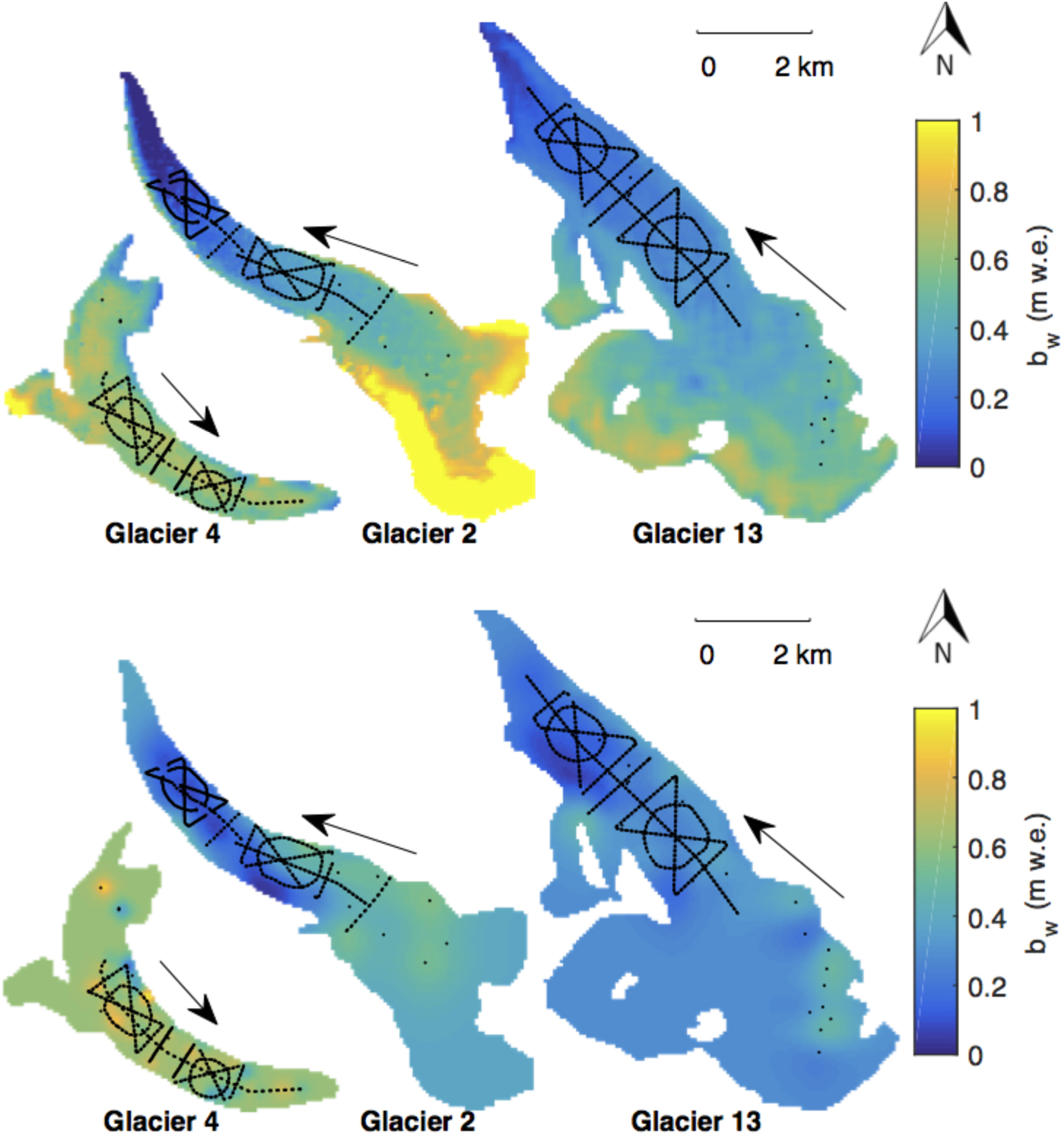
Fig. 4. Spatial distribution of winter balance (b w) estimated using linear regression (LR) (top row) and ordinary kriging (OK) (bottom row) with densities assigned as per S2 (Table 3). The LR method involves multiplying regression coefficients, found using cross validation and model averaging, by topographic parameters for each gridcell. OK uses the correlation of measured values to find a set of optimal weights for estimating values at unmeasured locations. Locations of snow-depth measurements made in May 2016 are shown as black dots. Ice-flow directions are indicated by arrows.
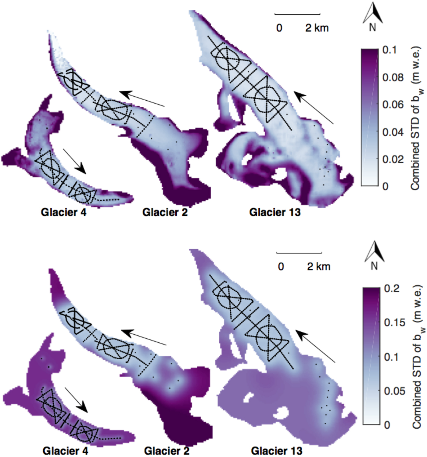
Fig. 5. Combined uncertainty of distributed winter balance (b w) for density-assignment method S2 (Fig. 4) found using linear regression (top row) and ordinary kriging (bottom row). Ice flow directions are indicated by arrows.
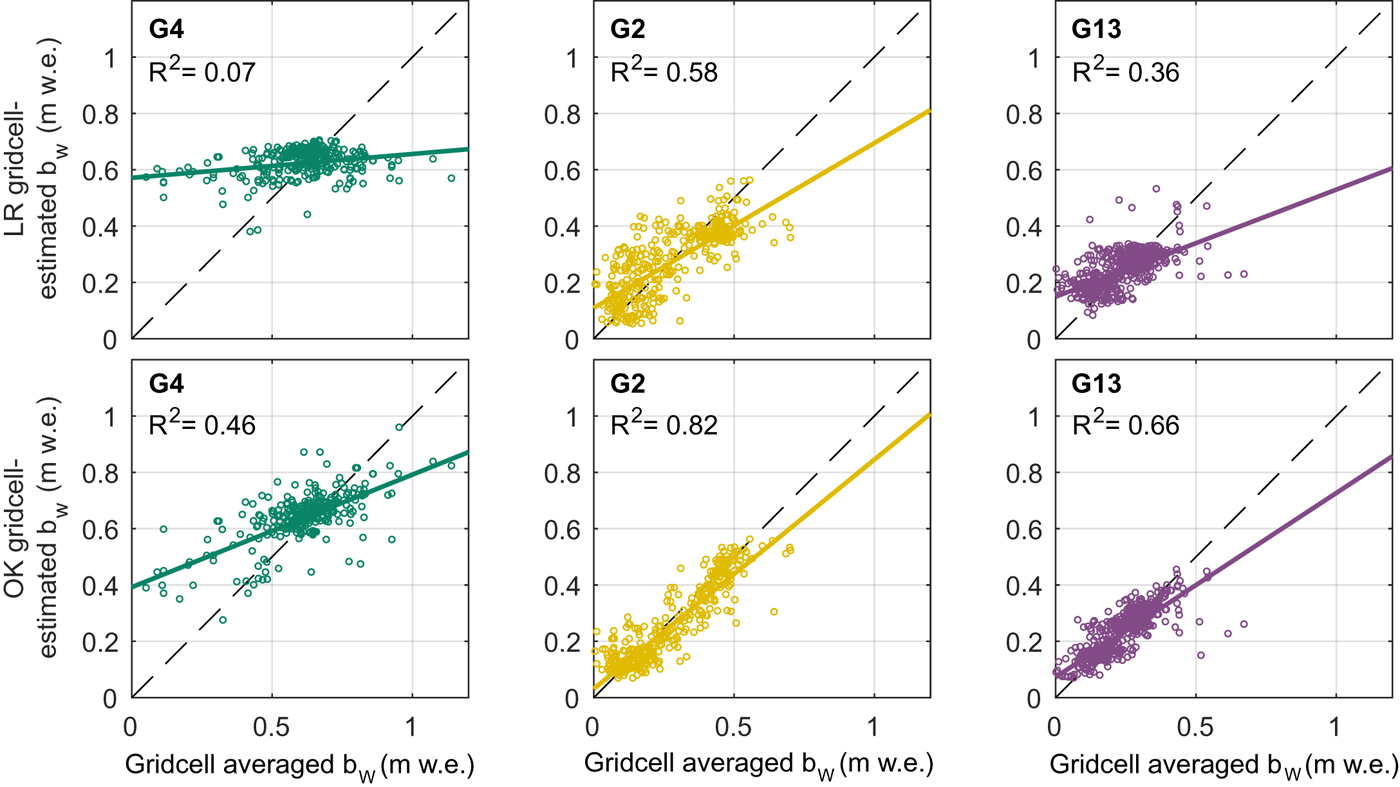
Fig. 6. Winter balance (b w) estimated by linear regression (LR, top row) or ordinary kriging (OK, bottom row) versus the gridcell-averaged b w data for Glacier 4 (left), Glacier 2 (middle) and Glacier 13 (right). Each circle represents a single gridcell. Explained variance (R 2) is provided. Best-fit (solid) and one-to-one (dashed) lines are shown.
Table 4. Glacier-wide winter balance (B w, m w.e.) estimated using linear regression and ordinary kriging for the three study glaciers (S2 density method). RMSE (m w.e.) is computed between gridcell-averaged values of b w (the data) that were randomly selected and excluded from interpolation (~ 1/3 of all data) and those estimated by interpolation. RMSE as a percent of B w is shown in parentheses

4.4.2. Ordinary kriging
For all three glaciers, large areas that correspond to locations far from measurements have b w estimates equal to the kriging mean. Distributed b w estimated with OK on Glacier 4 is mostly uniform except for local deviations close to measurement locations (Fig. 4) and combined uncertainty is high across the glacier. Distributed b w varies more smoothly on Glaciers 2 and 13 (Fig. 4). Glacier 2 has a distinct region of low estimated b w (~0.1 m w.e.) in the lower part of the ablation area, which corresponds to a wind-scoured region of the glacier. Glacier 13 has the lowest estimated mean b w and only small deviations from this mean at the measurement locations (Fig. 4). Combined uncertainty varies considerably across the three study glaciers with the greatest uncertainty far from measurement locations (Fig. 5). The variance explained by OK-estimated b w is high for Glaciers 2 and 13 relative to that for Glacier 4 (Fig. 6).
4.5. Uncertainty analysis using a Monte Carlo approach
Estimates of B w are affected by uncertainty introduced by the representativeness of gridcell-averaged values of b w (σ GS), choosing a method of density assignment (σ ρ), and interpolating/extrapolating b w values across the domain (σ INT). Using a Monte Carlo analysis, we find that interpolation uncertainty contributes more to B w uncertainty than grid-scale uncertainty or the method of density assignment (see Supplementary Material). In other words, the distribution of B w that arises from grid-scale uncertainty and the differences in distributions of B w due to different methods of density assignment are generally smaller than the distribution that arises from interpolation uncertainty (Fig. 7 and Table 5). B w distributions obtained using LR are strongly affected by extrapolation of positive linear relationships into the upper portion of the accumulation area. OK-estimated values of b w in the accumulation area are generally uniform (Fig. 4) but are sensitive to small variations in gridcell-averaged b w at locations along the edge of the survey. As a result, the uncertainty in OK-estimated values of B w is large, and unrealistic values (e.g. B w = 0 m w.e.) are possible (Fig. 7).
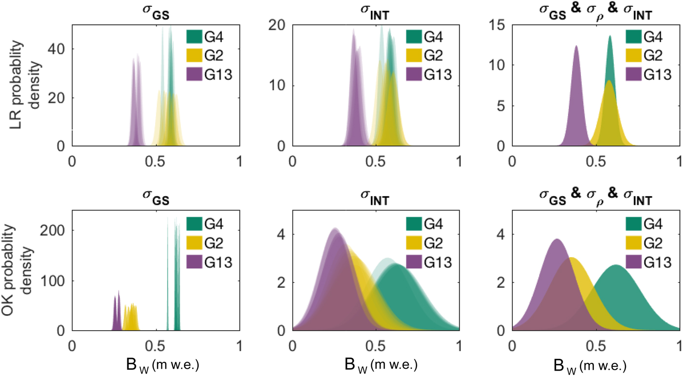
Fig. 7. Distributions of glacier-wide winter balance (B w) for Glaciers 4 (G4), 2 (G2) and 13 (G13) that arise from various sources of uncertainty. B w distribution arising from grid-scale uncertainty (σ GS) (left column). B w distribution arising from interpolation uncertainty (σ INT) (middle column). B w distribution arising from a combination of σ GS, σ INT and density assignment uncertainty (σ ρ) (right column). Results are shown for interpolation by linear regression (LR, top row) and ordinary kriging (OK, bottom row). Left two columns include eight distributions per glacier (colour) and each corresponds to a density assignment method (S1–S4 and F1–F4).
Table 5. Standard deviation (× 10−2 m w.e.) of glacier-wide winter balance (B w) distributions arising from uncertainties in grid-scale b w (σ GS), density assignment (σ ρ), interpolation (σ INT) and all three sources combined (σ ALL) for linear regression (left columns) and ordinary kriging (right columns)

The values of B w for our study glaciers (using LR and the S2 density assignment), with an uncertainty equal to one standard deviation of the distribution found with Monte Carlo analysis, are: 0.60 ± 0.03 m w.e. for Glacier 4, 0.52 ± 0.05 m w.e. for Glacier 2 and 0.39 ± 0.03 m w.e. for Glacier 13. The B w uncertainty from the three investigated sources of uncertainty ranges from 0.03 to 0.05 m w.e. (5–9%) for LR estimates and from 0.10 to 0.15 m w.e. (24–39%) for OK estimates.
5. DISCUSSION
5.1. Distributed winter balance
5.1.1. Linear regression
Of the topographic parameters in the LR, elevation (z) is the most significant predictor of gridcell-averaged b w for Glaciers 2 and 13, while wind redistribution (Sx) is the most significant predictor for Glacier 4 (Fig. 8). As expected, gridcell-averaged b w is positively correlated with elevation where the correlation is significant. It is possible that the elevation correlation was accentuated due to melt onset for Glacier 13 in particular. Glacier 2 had little snow at the terminus likely due to steep slopes and wind-scouring but the snow did not appear to have been affected by melt. Our results are consistent with many studies that have found elevation to be the most significant predictor of seasonal snow accumulation data (e.g. Machguth and others, Reference Machguth, Eisen, Paul and Hoelzle2006; Grünewald and others, Reference Grünewald, Bühler and Lehning2014; McGrath and others, Reference McGrath2015). The b w–elevation gradient is 13 mm w.e. 100 m−1 on Glacier 2 and 7 mm w.e. 100 m−1 on Glacier 13. These gradients are consistent with those reported for a few glaciers in Svalbard (Winther and others, Reference Winther, Bruland, Sand, Killingtveit and Marechal1998) but are considerably lower than many reported b w–elevation gradients, which range from ~60 to 240 mm w.e. 100 m−1 (e.g. Hagen and Liestøl, Reference Hagen and Liestøl1990; Tveit and Killingtveit, Reference Tveit and Killingtveit1994; Winther and others, Reference Winther, Bruland, Sand, Killingtveit and Marechal1998). Extrapolating linear relationships to unmeasured locations typically results in considerable estimation error, as seen by the large b w values (Fig. 4) and large combined uncertainty (Fig. 5) in the high-elevation regions of Glaciers 2 and 13. The low correlation between b w and elevation on Glacier 4 is consistent with Grabiec and others (Reference Grabiec, Puczko, Budzik and Gajek2011) and López-Moreno and others (Reference López-Moreno, Fassnacht, Beguería and Latron2011), who conclude that highly variable distributions of snow can be attributed to complex interactions between topography and the atmosphere that cannot be easily quantified. The snow on Glacier 4 also did not appear to have been affected by melt and it is hypothesized that significant wind-redistribution of snow, which was not captured by the Sx parameter, obscured ice topography and produced a relatively uniform snow depth across the glacier.
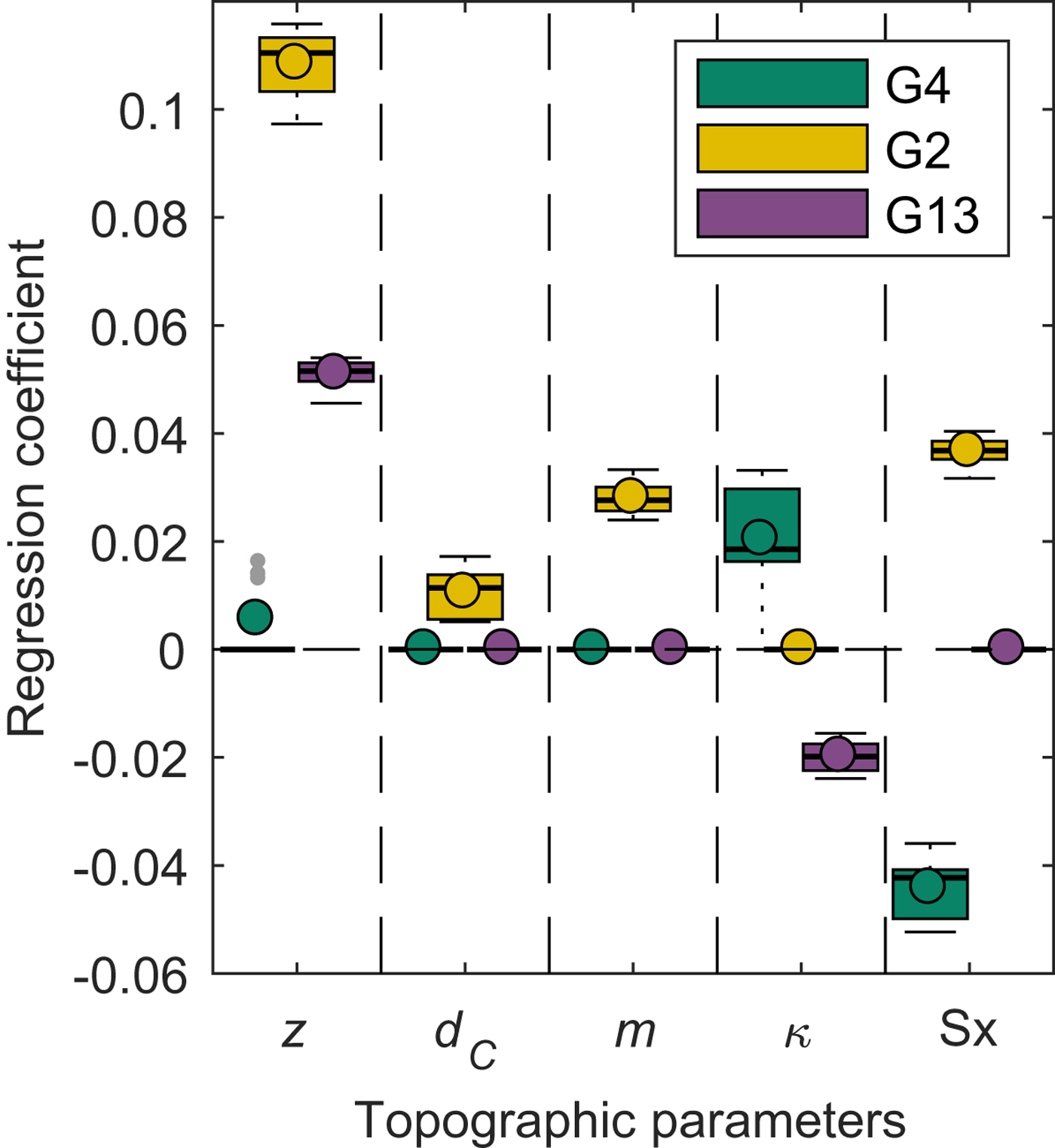
Fig. 8. Distribution of coefficients (β) determined by linear regression of gridcell-averaged b w on DEM-derived topographic parameters for the eight different density assignment methods (Table 3). Coefficients are calculated using standardized data, so values can be compared across parameters. Regression coefficients that are not significant are assigned a value of zero. Topographic parameters include elevation (z), distance from centreline (d C), slope (m), curvature (κ) and wind redistribution (Sx). Aspect and ‘northness’ are not shown because coefficient values are zero in every case. The box plot shows first quartiles (box), median (line within box), mean (circle within box), minimum and maximum values excluding outliers (bars) and outliers (gray dots), which are defined as being outside of the range of 1.5 times the quartiles (~± 2.7σ).
Gridcell-averaged b w is negatively correlated with Sx on Glacier 4, counter-intuitively indicating less snow in what would be interpreted as sheltered areas. Gridcell-averaged b w is positively correlated with Sx on Glaciers 2 and 13. Our results corroborate those of McGrath and others (Reference McGrath2015) in a study of six glaciers in Alaska (DEM resolutions of 5 m) where elevation and Sx were the only significant parameters for all glaciers; Sx regression coefficients were smaller than elevation regression coefficients, and in some cases, negative. While our results point to wind having an impact on snow distribution, the wind redistribution parameter (Sx) may not adequately capture these effects at our study sites. For example, Glacier 4 has a curvilinear plan-view profile and is surrounded by steep valley walls, so specifying a single cardinal direction for wind may not be adequate. Further, the scale of deposition may be smaller than the resolution of the Sx parameter estimated from the DEM. Creation of a parametrization for sublimation from blowing snow, which has been shown to be an important mechanism of mass loss from ridges (e.g. Musselman and others, Reference Musselman, Pomeroy, Essery and Leroux2015), may also increase the explanatory power of LR for our study sites.
We find that transfer of LR coefficients between glaciers results in large estimation errors. Regression coefficients from Glacier 4 produce the highest RMSE (0.38 m w.e. on Glacier 2 and 0.40 m w.e. on Glacier 13, see Table 4 for comparison) and B w values are the same for all glaciers (0.64 m w.e.) due to the dominance of the regression intercept. Even if the LR is performed with b w values from all glaciers combined, the resulting coefficients produce large RMSE when applied to individual glaciers (0.31 m w.e., 0.15 m w.e. and 0.14 m w.e. for Glaciers 4, 2 and 13, respectively). Our results are consistent with those of Grünewald and others (Reference Grünewald2013), who found that local statistical models cannot be transferred across basins and that regional-scale models are not able to explain the majority of observed variance in winter balance.
5.1.2. Ordinary kriging
Due to a paucity of data, OK produces almost uniform gridcell-estimated b w in the accumulation area of each glacier, inconsistent with observations described in the literature (e.g. Machguth and others, Reference Machguth, Eisen, Paul and Hoelzle2006; Grabiec and others, Reference Grabiec, Puczko, Budzik and Gajek2011). Glacier 4 has the highest estimated mean with large deviations from the mean at measurement locations. The longer correlation lengths of the data for Glaciers 2 and 13 result in a more smoothly varying distributed b w. As expected, extrapolation using OK leads to large uncertainty (Fig. 5), further emphasizing the need for spatially distributed point-scale measurements.
5.1.3. Sensitivity of winter balance to interpolation/extrapolation method
The physically-based LR estimates and the statistically-based OK estimates result in different distributions of b w for the three study glaciers (Fig. 4). Since LR is based on physical parameters, extrapolation to areas with extreme values of these parameters can lead to sharp changes in estimated b w and to large uncertainty (Fig. 7), due to the sensitivity of the regression to each topographic parameter. The accumulation areas of Glaciers 2 and 13 have large estimated b w values because observations are sparse and topographic parameters, such as elevation, attain their highest values.
In contrast, OK tends to result in extrapolated values of b w that approach the data mean and are smoothly varying. For Glaciers 2 and 13, OK estimates are more than ~0.22 m w.e. (39%) and ~0.11 m w.e. (30%) lower than LR estimates, respectively (Table 4). The influence of elevation results in substantially higher LR-estimated values of b w at high elevation, whereas OK-estimated values are more uniform. Since OK is a data-fitting interpolation method, the absolute RMSE of OK is ~0.03 m w.e. lower for all glaciers (Table 4).
These two different methods produce similar estimates of distributed b w (Fig. 4) and B w (~0.6 m w.e., Table 4) on Glacier 4, but both are relatively poor predictors of b w in measured gridcells (Fig. 6). Additionally, RMSEs as a percentage of glacier-wide B w are comparable between LR and OK (Table 4) with an average RMSE of 21%. This comparability is interesting, given that all of the data were used to generate the OK model, while only ~ 2/3 were used in the LR. Tests in which only ~ 2/3 of the data were used in the OK model yielded similar results to those in which all data were used.
5.2. Uncertainty analysis using a Monte Carlo approach
Interpolation/extrapolation of b w data is the largest contributor to b w uncertainty in our study. These results caution strongly against including interpolated/extrapolated values of b w in comparisons with remote sensing- or model-derived estimates of b w. If possible, such comparisons should be restricted to point-scale data. Grid-scale uncertainty (σ GS) is the smallest assessed contributor to overall B w uncertainty. This result is consistent with the generally smoothly-varying snow depths encountered in zigzag surveys, and previously reported ice-roughness lengths on the order of centimetres (e.g. Hock, Reference Hock2005) compared with snow depths on the order of decimetres to metres. Given our assumption that zigzags are an adequate representation of grid-scale variability, the low B w uncertainty arising from σ GS implies that subgrid-scale sampling need not be a high priority for reducing overall uncertainty. Our assumption that the 3–4 zigzag surveys can be used to estimate glacier-wide σ GS may be flawed, particularly in areas with debris cover, crevasses and steep slopes.
Our analysis did not include uncertainty arising from density measurement errors associated with the FS, wedge cutters and spring scales, from vertical and horizontal errors in the DEM or from the error associated with estimating measurement locations based on the GPS position of the lead observer. We assume that these sources of uncertainty are either encompassed by the sources investigated or are negligible.
5.3. Regional winter-balance gradient
Although we find considerable inter- and intra-basin variability in winter balance, our results are consistent with a regional-scale winter-balance gradient for the continental side of the St. Elias Mountains (Fig. 9). Winter-balance data are compiled from Taylor-Barge (Reference Taylor-Barge1969), the three glaciers presented in this paper and two snow pits we analyzed near the head of the Kaskawulsh Glacier between 20 and 21 May 2016. The data show a linear decrease of 0.024 m w.e. km−1 (R 2 = 0.85) in winter balance with distance from the regional topographic divide between the Kaskawulsh and Hubbard Glaciers, as identified by Taylor-Barge (Reference Taylor-Barge1969). While the three study glaciers fit the regional trend, the same relationship would not apply if just the Donjek Range were considered. We hypothesize that interaction between meso-scale weather patterns and large-scale mountain topography is a major driver of regional-scale winter balance. Further insight into regional-scale patterns of winter balance in the St. Elias Mountains could be gained by investigating moisture source trajectories and the contribution of orographic precipitation.
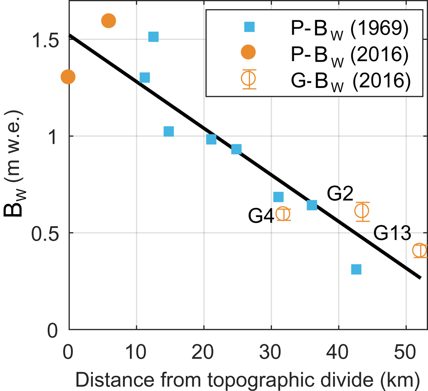
Fig. 9. Relationship between winter balance (B w) and linear distance from the regional topographic divide between the Kaskawulsh and Hubbard Glaciers in the St. Elias Mountains. Point-scale values of winter balance from snow-pit data reported by Taylor-Barge (Reference Taylor-Barge1969) (blue boxes, P-B w). LR-estimated B w calculated using density assignment S2 for Glaciers 4 (G4), 2 (G2) and 13 (G13) with errors bars calculated as the standard deviation of Monte Carlo-derived B w distributions (this study) (open orange circles, G-B w). Point-scale B w estimated from snow-pit data at two locations in the accumulation area of the Kaskawulsh Glacier, collected in May 2016 (unpublished data, SFU Glaciology Group) (filled orange dots, P-B w). Black line indicates best fit (R 2 = 0.85).
5.4. Limitations and future work
The potential limitations of our work include the restriction of our data to a single year, minimal sampling in the accumulation area, the problem of uncorrelated SP- and FS-derived densities, a sampling design that could not be optimized a priori, the assumption of spatially uniform subgrid variability and lack of more finely resolved DEMs.
Interannual variability in winter balance is not considered in our study. A number of studies have found temporal stability in spatial patterns of snow distribution and that statistical models based on topographic parameters could be applied reliably between years (e.g. Grünewald and others, Reference Grünewald2013). For example, Walmsley (Reference Walmsley2015) analyzed more than 40 years of winter balance recorded on two Norwegian glaciers and found that snow distribution is spatially heterogeneous yet exhibits robust temporal stability. Contrary to this, Crochet and others (Reference Crochet2007) found that snow distribution in Iceland differed considerably between years and depended primarily on the dominant wind direction over the course of a winter. Therefore, multiple years of snow depth and density measurements are needed to better understand interannual variability of winter balance within the Donjek Range.
There is a conspicuous lack of data in the accumulation areas of our study glaciers. With increased sampling in the accumulation area, interpolation uncertainties would be reduced where they are currently greatest and the LR would be better constrained. Although certain regions of the glaciers remain inaccessible for direct measurements, other methods of obtaining winter-balance measurements, including ground-penetrating radar and DEM differencing with photogrammetry or lidar, could be used in conjunction with manual probing to increase the spatial coverage of measurements.
The lack of correlation between SP- and FS-derived densities needs to be reconciled. Contrary to our results, most studies that compare SP- and FS-derived densities report minimal discrepancy (e.g. Dixon and Boon, Reference Dixon and Boon2012, and sources within). Additional co-located density measurements are needed to better compare the two methods of obtaining density values. Comparison with other FS would also be informative. Even with this limitation, density assignment was, fortunately, not the largest source of uncertainty in estimating glacier-wide winter balance.
Our sampling design was chosen to achieve broad spatial coverage of the ablation area, but is likely too finely resolved along transects for many mass-balance surveys to replicate. An optimal sampling design would minimize uncertainty in winter balance while reducing the number of required measurements. Analysis of the estimated winter balance obtained using subsets of the data is underway to make recommendations on optimal transect configuration and along-track spacing of measurements. López-Moreno and others (Reference López-Moreno, Latron and Lehmann2010) found that 200–400 observations are needed within a non-glacierized alpine basin (6 km2) to obtain accurate and robust snow distribution models. Similar guidelines would be useful for glacierized environments.
In this study, we assume that the subgrid variability of winter balance is uniform across a given glacier. Contrary to this assumption, McGrath and others (Reference McGrath2015) found greater variability of winter-balance values close to the terminus. Testing our assumption could be a simple matter of prioritizing the labour-intensive zigzags surveys. To ensure consistent quantification of subgrid variability, zigzag survey measurements could also be tested against other measurements methods, such as lidar.
DEM gridcell size is known to influence values of computed topographic parameters (Zhang and Montgomery, Reference Zhang and Montgomery1994; Garbrecht and Martz, Reference Garbrecht and Martz1994; Guo-an and others, Reference Guo-an, Yang-he, Strobl and Wang-qing2001; López-Moreno and others, Reference López-Moreno, Latron and Lehmann2010). The relationship between topographic parameters and winter balance is, therefore, not independent of DEM gridcell size. For example, Kienzle (Reference Kienzle2004) and López-Moreno and others (Reference López-Moreno, Latron and Lehmann2010) found that a decrease in spatial resolution of the DEM results in a decrease in the importance of curvature and an increase in the importance of elevation in LR of snow distribution on topographic parameters in non-glacierized basins. The importance of curvature in our study is affected by the DEM smoothing that we applied to obtain a spatially continuous curvature field (see Supplementary Material, Fig. S1). A comparison of regression coefficients from high-resolution DEMs obtained from various sources and sampled with various gridcell sizes could be used to characterize the dependence of topographic parameters on DEMs, and therefore assess the robustness of inferred relationships between winter balance and topographic parameters.
6. CONCLUSION
We estimate winter balance for three glaciers (termed Glacier 2, Glacier 4 and Glacier 13) in the St. Elias Mountains, Yukon, Canada from multiscale snow depth and density measurements. Linear regression and ordinary kriging are used to obtain estimates of distributed winter balance (b w). We use Monte Carlo analysis to evaluate the contributions of interpolation, assignment of snow density and grid-scale variability of winter balance to uncertainty in estimates of glacier-wide winter balance (B w).
Values of B w estimated using LR and OK differ by up to 0.18 m w.e. We find that interpolation uncertainty is the largest assessed source of uncertainty in B w (5–9% for LR estimates and 24–39% for OK estimates). Uncertainty resulting from the method of density assignment is comparatively low, despite the wide range of methods explored. Given our representation of grid-scale variability, the resulting B w uncertainty is small indicating that extensive subgrid-scale sampling is not required to reduce overall uncertainty.
Our results suggest that processes governing distributed b w differ between glaciers, highlighting the importance of regional-scale winter-balance studies. On Glacier 4, measured values of b w are characterized by high variability with many outliers, leading to poor correlation with estimated values. Measured values on Glacier 2 and 13 were less variable, with elevation being a significant predictor of gridcell-averaged b w. A wind-redistribution parameter is found to be a weak but significant predictor of b w, though conflicting relationships between glaciers make it difficult to interpret. The major limitations of our work include the restriction of our data to a single year and minimal sampling in the accumulation area. Although challenges persist when estimating winter balance, our data are consistent with a regional-scale winter-balance gradient for the continental side of the St. Elias Mountains.
7. AUTHOR CONTRIBUTION STATEMENT
AP planned and executed the data collection, performed all calculations and analysis and drafted and edited the manuscript. GF conceived of the study, contributed to field planning and data collection, oversaw all stages of the work and edited the manuscript. VR provided guidance on the methods of data analysis and edited the manuscript. DB provided insight into the statistical analysis and edited the manuscript.
SUPPLEMENTARY MATERIAL
The supplementary material for this article can be found at https://doi.org/10.1017/jog.2018.68
ACKNOWLEDGMENTS
We thank the Kluane First Nation (KFN), Parks Canada and the Yukon Government for granting us permission to work in KFN Traditional Territory and Kluane National Park and Reserve. We are grateful for financial support provided by the Natural Sciences and Engineering Research Council of Canada, Simon Fraser University and the Northern Scientific Training Program. We kindly acknowledge Sian Williams, Lance Goodwin and pilot Dion Parker for facilitating field logistics. We are grateful to Alison Criscitiello and Coline Ariagno for all aspects of field assistance and Sarah Furney for assistance with data entry. Thank you to Etienne Berthier for providing us with the SPIRIT SPOT-5 DEM and for assistance in DEM correction. We are grateful to Michael Grosskopf for assistance with the statistics, including OK. Luke Wonneck, Leif Anderson and Jeff Crompton all provided constructive comments on drafts of the manuscript. We appreciate the thoughtful input of two anonymous reviewers.


 Open access