


1. Introduction
More than 600 known Antarctic subglacial lakes (Livingstone and others, Reference Livingstone2022) form a key component of the basal hydrological system; they influence ice dynamics, are an extreme habitable environment (Couston and Siegert, Reference Couston and Siegert2021) with potential for evolutionary isolation, and if long-lived may host unique sediment records of ice-sheet history. As such, despite their inaccessibility, subglacial lakes have attracted a significant amount of interest in recent years. All lakes recognised to date have been identified by bright specular reflectors in radar surveys, by their distinctive flat ice surface manifestation or by surface elevation changes as they drain and refill. Although the areal extent of lakes can be constrained by radar or satellite surveys, water depth and hence water body volume cannot be delineated with those methods. Gravity surveys have been used to constrain water depth but with significant uncertainties (Thoma and others, Reference Thoma, Grosfeld, Filina and Mayer2009; Tikku and others, Reference Tikku2017). Hence, only seismic measurements can unambiguously constrain water column thickness (Kapitsa and others, Reference Kapitsa, Ridley, de Robin, Siegert and Zotikov1996; Brisbourne and others, Reference Brisbourne2014). Furthermore, properties of the lakebed, key to further subglacial investigations, are uniquely determined by seismic surveys. Many Antarctic subglacial lakes lie close to the ice divides in steep-sided and deeply incised valleys beneath kilometres of ice, where seismic measurements are technically challenging and often restricted due to the constrained raypath geometries associated with such topography. As such, only subglacial Lakes Vostok (Filina and others, Reference Filina2008), Ellsworth (Woodward and others, Reference Woodward2010), Whillans (Horgan and others, Reference Horgan2012) and South Pole (Peters and others, Reference Peters2008) have water depths from seismic measurements to date. Reported lake depths range from 8 m at Lake Whillans, 32 m at South Pole, up to 156 m at Lake Ellsworth and 1067 m at Lake Vostok.
Recent success in directly accessing subglacial lakes has been reported (Christner and others, Reference Christner2014; Lukin and Vasiliev, Reference Lukin and Vasiliev2014; Tulaczyk and others, Reference Tulaczyk2014; Priscu and others, Reference Priscu2021). However, direct access to Lake Vostok did not recover sediment and that recovered from Lakes Whillans and Mercer reflect glacial flow processes and not subglacial lake sedimentation (Hodson and others, Reference Hodson, Powell, Brachfeld, Tulaczyk and Scherer2016; Siegfried and others, Reference Siegfried2023). Lakes Whillans and Mercer are two of a series of interconnected subglacial lakes at the confluence of the Whillans and Mercer Ice Streams. Lake Whillans (SLW) was accessed in 2013. At the SLW drill site, water column thickness was ~2 m, less than the 8 ± 2 m inferred by the seismic survey. Samples of sediment from the lake bed indicate intermittent flood events that lead to grounding of the ice sheet and till formation at the bed. Salinity of the lake water was measured at 100 times less than sea water. Lake Mercer is influenced by drain/fill cycles of Conway Subglacial Lake immediately upstream (Carter and others, Reference Carter, Fricker and Siegfried2013). Lake Mercer, with a water depth of ~15 m, was accessed in 2018 through 1087 m of ice. Lake water and sediment samples were recovered (Priscu and others, Reference Priscu2021). Basal ice was observed to contain entrained sediment. Grain size analysis of sediment samples from the lake bed indicate a similar distribution to glacial till sampled elsewhere in the region. Again, lake water salinity is reported as 100 times less than sea water but an order of magnitude more saline than Lake Vostok.
Lago Subglacial CECs (hereafter SLC) lies at the ice divide between the Rutford Ice Stream, Institute Ice Stream and Minnesota Glacier in the Ellsworth Highlands region of Antarctica (Figs 1a, b; Napoleoni and others, Reference Napoleoni2020). Rivera and others (Reference Rivera, Uribe, Zamora and Oberreuter2015) report a fresh water lake with a surface area of 18 km2, at 609 m below geoid height and beneath 2653 m of ice, with low ice flow at the surface (1.0 ± 0.2 m a−1), and calculate the pressure melting point at the ice–lake interface of −1.8°C. Repeated survey of a stake network installed in 2014 indicates an annual surface accumulation of 0.14–0.20 m w.e. Negligible surface elevation change (Rivera and others, Reference Rivera, Uribe, Zamora and Oberreuter2015) indicates that SLC is likely part of a stable system with long water residence time. This is in contrast to Lakes Whillans and Mercer for example, which are termed active lakes, undergoing intermittent drainage and refill events.
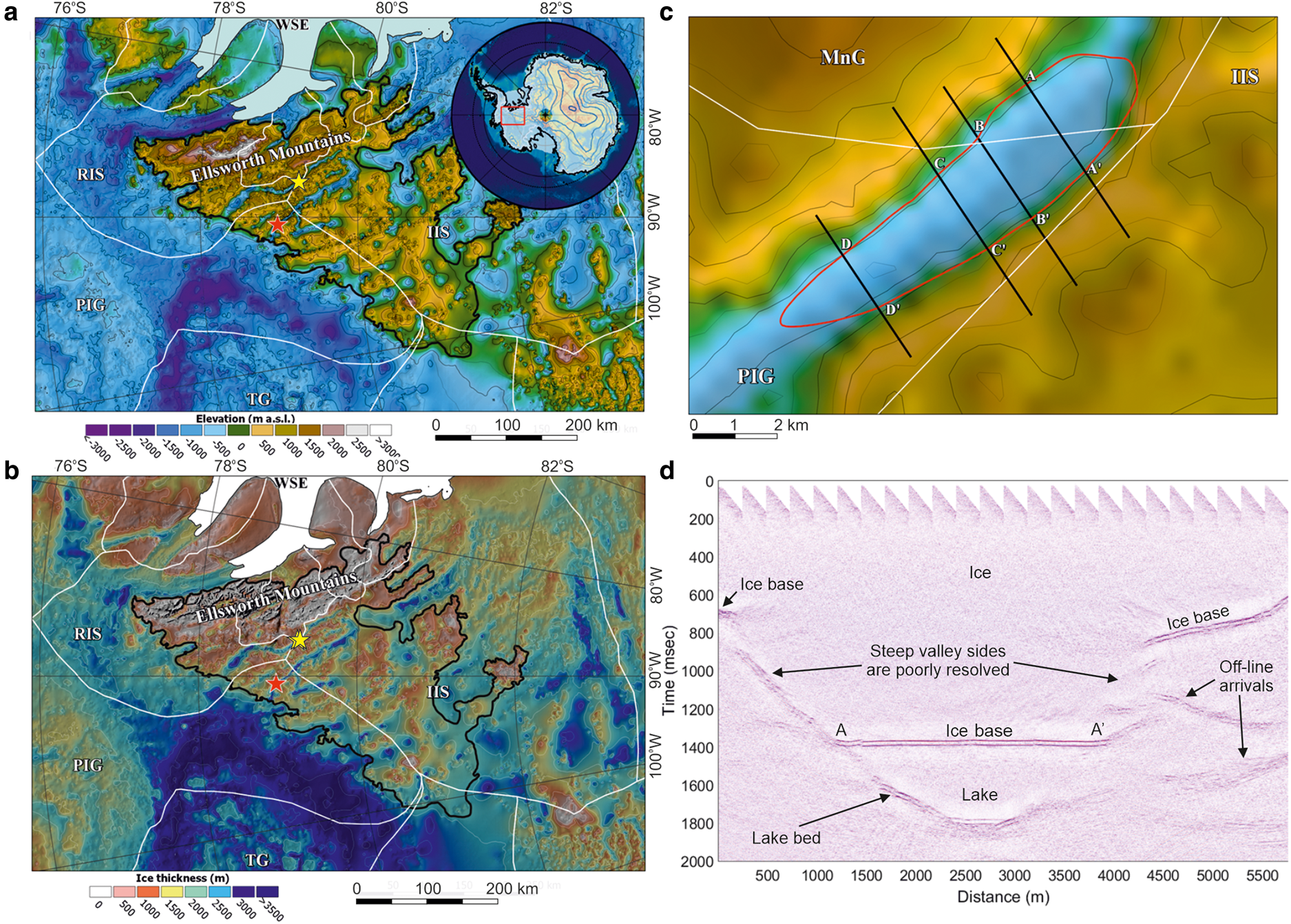
Figure 1. (a) Location of SLC (yellow star) and Subglacial Lake Ellsworth (red star) within the Ellsworth Subglacial Highlands, West Antarctica (black outline). The background is the DEMESH bed elevation model (Napoleoni, Reference Napoleoni2020). White lines are the MEaSUREs Antarctic ice stream basin boundaries (Mouginot and others, Reference Mouginot, Scheuchl and Rignot2017) (RIS, Rutford Ice Stream; PIG, Pine Island Glacier; TG, Thwaites Glacier; IIS, Institute Ice Stream; WSE, Weddell Sea Embayment). The inset shows the location within Antarctica with surface elevation. (b) As (a) but with ice thickness with contours at 500 m intervals (Napoleoni, Reference Napoleoni2020). (c) Ice base elevation with contours at 100 m interval in brown (colour scale as in a) and the outline of SLC in red, determined from radar and seismic data (centred at 79.23°S, 087.62°W). Black lines indicate the four seismic profiles with the orientation identifiers used in Figure 2 (MnG, Minnesota Glacier). (d) Seismic profile A with automatic gain control applied showing full ice overburden and lake profile. With the display in seismic two-way travel time, the lake depth profile is exaggerated in the image due to the low P-wave velocity in water compared to ice.

Figure 2. Seismic sections highlighting the lake profile scaled with identical vertical exaggeration (5:1). Amplitudes in the seismic profiles are normalised to optimise the images. Example ice–water and lake bed wavelets are included as insets on profile A from points outlined by the black boxes on the interface. For reference, wavelets from the ice–bed interface at 4700 m along profile A (Fig. 1d) are presented. The black bars indicate 100 m equivalent vertical water column thickness, assuming the P-wave velocity of fresh water. The 3-D plot presents the lake surface and depth profile determined from the seismic sections and surface radar profiles, displayed without vertical exaggeration. Maximum water column thickness increases from 80 m on profile D to 301 m on profile A. The lake surface and lakebed picks are in black and the projected lake surface outline is in red. The red arrow indicates the direction of lake outflow path (Rivera and others, Reference Rivera, Uribe, Zamora and Oberreuter2015) at the south-eastern end of the lake. Inverted triangles indicate discontinuities in the seismic reflection from the ice base (top of the lake) which are likely due to 3-D structure of the ice–water interface which is not fully resolved by our 2-D methods.
SLC lies at the base of a deep subglacial fjord-like linear trough (Fig. 1a) that likely evolved through glacial and fluvial erosion, controlled by tectonic structure, prior to the current glacial period (Vaughan and others, Reference Vaughan2007; Jamieson and others, Reference Jamieson2014; Ross and others, Reference Ross2014; Sugden and others, Reference Sugden2017; Napoleoni and others, Reference Napoleoni2020). SLC is adjacent to the Heritage Range of the Ellsworth Mountains which is composed of predominantly clastic sedimentary and volcanic rock formations (Curtis, Reference Curtis2001). Further west of SLC, at Mt Johns, quartzite is outcropping (Anderson, Reference Anderson1960). Aero-geophysical data suggest similar bedrock across the region (Jankowski and Drewry, Reference Jankowski and Drewry1981).
To understand the physical processes and conditions in subglacial lakes, and to evaluate the suitability of this particular lake for further exploration via direct access, knowledge of lake bathymetry and bed conditions is necessary. Here, we present results of seismic surveys targeting water column thickness and lakebed properties of SLC.
2. Data and methods
The lake extent was derived previously using extensive radar data (Rivera and others, Reference Rivera, Uribe, Zamora and Oberreuter2015), and further refined here by subsequent surveys (Fig. 1c). Three seismic reflection lines were acquired across the lake in December 2016 (profiles A, C and D) and an additional line in January 2022 (profile B). Profile A is at the wider south-eastern end of the lake and profile D at the narrow north-western end. A seismic source of 450 g of high explosives was deployed in 20 m holes. A shot interval of 240 m with 48 receivers at 10 m intervals and 30 m offset was used to produce single-fold normal-incidence (<10° incidence angle) data with a nominal trace midpoint interval of 5 m. Data were recorded at 8000 Hz with a 4 s record length. To determine lake geometry and basal properties, data processing includes normal moveout correction and 2-D Kirchoff time migration.
Traveltimes to the ice–water interface, measured directly from the migrated seismic section, are converted to depth using estimates of seismic velocities in the firn and ice column. Velocities in the firn are determined from seismic refraction measurements (Kirchner and Bentley, Reference Kirchner, Bentley, Bentley and Hayes1990). Assuming a linear temperature profile from the surface to the base (−25 to −1.8°C) and the temperature–velocity relationship of Kohnen (Reference Kohnen1974), a mean velocity of the ice column of 3826 m s−1 was determined. The water column thickness is calculated from the traveltime difference between the ice base and lakebed reflections assuming a P-wave velocity in fresh water of 1437 m s−1.
We measure reflection amplitudes of the ice base and lake bed directly using the migrated seismic profiles. We follow the recommendations of Horgan and others (Reference Horgan2021) and measure root-mean-squared amplitudes of the wavelet, which includes the central peak and both side lobes (example wavelets in Fig. 2). The reflection coefficient at the ice base (R 1) can be calculated using assumed values of seismic velocity and density of basal ice (v i = 3800 ± 10 m s−1 and ρ i = 917 ± 2 kg m−3) and fresh water (v w = 1437 ± 2 m s−1 and ρ w = 1009 ± 5 kg m−3 (Rivera and others, Reference Rivera, Uribe, Zamora and Oberreuter2015)).

The product of seismic velocity and density (vρ) is termed the acoustic impedance (Z). The amplitude of the ice–water reflection can then be used to determine the reflection coefficient at the lake bed following Robin (Reference Robin1958). The reflection coefficient at the lake bed (R 2) can be derived from the amplitude ratio of the ice–water (A 1) and water–lakebed (A 2) reflections by

where h i and h w are the ice and water column thickness, respectively. By assuming the density and seismic velocity of the lake water, the reflection coefficient at the lakebed is used to calculate the acoustic impedance of the material at the lakebed, which in turn can be used to infer the lakebed properties. Attenuation in the water column is assumed to be zero. Uncertainties in the lake bed acoustic impedance measurements are dominated by those of the assumed values of density and P-wave velocity of basal ice and lake water. We propagate uncertainties through to the calculated values of acoustic impedance using standard methods.
We extend this method to determine the acoustic impedance of a reflector within the bed. Again, following Robin (Reference Robin1958), we use the amplitude of the sub-bed reflector (A 3) to determine the reflection coefficient using:

where A 3 is the sub-bed reflection amplitude and h b is the bed thickness. We must also consider the effect of seismic attenuation (α) in the bed. No measurements of seismic attenuation within subglacial lake bed materials exist. We therefore use the analogy of marine sediments and assume an attenuation value range consistent with seismic quality factor (Q) of 60 ± 20 where Q = πf/αv for frequency f (Eddies, Reference Eddies1994). As with the lakebed, the reflection coefficient of the sub-bed reflector may then be used to calculate the acoustic impedance of the material beneath the sub-bed reflector, using the acoustic impedance values calculated at the lakebed. As the seismic velocity and attenuation in the bed material is less well constrained than in ice and water, and the calibration is dependent on the reflection coefficients calculated for the interfaces above, the uncertainties become greater than for the shallower interfaces.
3. Results
Seismic profile A, presented in Figure 1d, highlights the difficulties in imaging the steep sub-glacial topography. At the extreme ends of profile A the ice is relatively thin, at ~1300 m (700 ms two way time), and its base gently sloping. However, towards the centre of the profile, the valley sides plunge towards the lake surface, with an elevation drop of ~1300 m over 1000 m horizontally at the NE end, and 1000 m over only ~300 m at the SW end, indicating mean slopes of 43° and 73° respectively. Although seismic arrivals appear to be consistent with the steep valley sides, closer examination of the geometry and frequency spectra of the waveforms indicate that these are likely to be a result of 3-D structure which cannot be resolved by our 2-D acquisition geometry, or poorly migrated energy.
Figure 2 presents seismic sections centred on the lake profile along with a 3-D representation of the lake depth profile. The lake surface reflection is clear on all seismic lines due to the high contrast in acoustic impedance between ice and water (Fig. 2). Discontinuities are observed in the seismic reflection from the lake surface, for example, at distance ~3200 and ~3800 m on profile C. We attribute these features to 3-D topography of the ice–water interface, which is again not fully resolved by our 2-D surveys and data processing. This implies that, at these locations, the three dimensional topography is more irregular than the lake surface elsewhere. We see a similar feature at the margin of the lake on profile A (at distance 1200–1400 m) where 3-D topography creates discontinuities in the ice base reflection (Fig. 2). These features are coincident with dimming in the ice base reflection in radar profiles across the lake. They may be small ice-base irregularities inherited from earlier grounded ice flow or else be an indication of ice–water interaction variations related to complexities in lake circulation. Additional data and ray-trace modelling would be needed to investigate these features further.
In general the lakebed profiles consist of a central flat or gently dipping section with the margins dipping more steeply up towards the ice base. Along profile A, this central section is characteristically flat and smooth and with no seismic reflections directly beneath the lake bed reflector. Along profiles B, C and D, this central section is narrower and less well defined and indicates more topography and greater internal reflectivity within the lake bed. The lakebed reflection is generally weaker than the lake surface reflection and, although identifiable over most of the central section of the lake, becomes difficult to distinguish along the steep sides. A 200 m long strong, dipping reflector, close to the bottom of the lake and of greater amplitude than the ice–water interface, is observed consistently on profiles A, B and C (Fig. 3). The gentler slopes of the lakebed along profile D are more readily imaged in the seismic data but this strong dipping reflection is absent.

Figure 3. Seismic profiles highlighting details of the lakebed with acoustic impedance (Zb) measurements at the lakebed (in units of ×106 kg m−2 s−1). Amplitudes in the seismic profiles are normalised to optimise images. The black line represents the mean acoustic impedance and in grey are the uncertainties propagated from measurement errors and the likely range of ice and water density and P-wave velocity. The blue dashed line indicates the acoustic impedance of water and the brown band that of high-porosity silt- and clay-dominated sediments (Smith and others, Reference Smith2018). For reference, calculated acoustic impedance values of lithified sediment and bedrock, at 9.2 and 14.0 × 10⁶ kg m−2 s−1 respectively (Peters and others, Reference Peters2008), are beyond the y-axis scale presented here. The direction of the lake outflow derived from the hydrological potential is into the page (Rivera and others, Reference Rivera, Uribe, Zamora and Oberreuter2015).
Profile A straddles the widest part of the lake and the maximum water column thickness of 301.3 ± 1.5 m is measured. Water column thickness tapers along the length of the lake with maximum thickness on profiles B, C and D of 254.3, 199.8 and 80.1 ± 1.5 m, respectively. Uncertainties in water column thickness result from uncertainties in traveltime picks and the seismic velocity in the water. Although all seismic lines extend onto grounded ice beyond the edges of the lake (e.g. Fig. 1c), the data quality is inadequate to determine the acoustic impedance of the bed beyond the lake due to the acquisition geometry, steepness of the topography and coincident off-profile reflections. For example, the strong ice-base reflection at 4000–5500 m on profile A exhibits a complex and highly variable primary wavelet which precludes reliable measurement of the acoustic impedance at this location. This complexity in the waveform is attributed to 3-D topography across this area or varying thin bed effects. Water column thickness increases towards the wider south-eastern end of the lake, where hydrological modelling indicates potential outflow of subglacial water under the current ice-sheet configuration (Rivera and others, Reference Rivera, Uribe, Zamora and Oberreuter2015). The limited seismic data do not constrain the full extent of the lake surface. We therefore extrapolate the lake surface picks from the seismic data using the lake surface perimeter determined from radar measurements. Likewise, we also linearly interpolate the lakebed between the seismic picks and the radar-derived lake perimeter to derive an interpolated grid of the lakebed (Fig. 2). Using this derived lake surface and bed topography, we determine a lake surface area of 18.7 km2 (4% greater than Rivera and others (Reference Rivera, Uribe, Zamora and Oberreuter2015)) and lake volume of 2.5 ± 0.3 km3. Uncertainties in the lake volume calculation are difficult to quantify as we are extrapolating over considerable distances and beyond known depth measurements; hence, a conservative error is quoted here. Further radar and seismic data will allow better estimates of both the lake volume and its uncertainty.
In Figure 3, we present the seismic profiles focused on the lake bed and measured lake bed acoustic impedance with uncertainties. As SLC is located in the interior of the ice sheet, has a considerable water depth sitting at the bottom of a deep subglacial fjord and shows no indications of any short-term variability, we consider the derived acoustic impedance values in terms of a subglacial lacustrine environment. For reference, we indicate the acoustic impedance values of water (blue-dashed line) and high-porosity fine-grained sub-aqueous sediment (brown band) (Smith and others, Reference Smith2018). Measurement errors and the uncertainties in the assumed values of density and P-wave velocity of basal ice and lake water are propagated through to the calculated values of acoustic impedance presented in Figure 3. The assumed values of velocity and density are likely to be consistent across the lake and we therefore refer to the mean values and their variance when comparing between profiles.
Consistent on profiles A, B and C, a strong dipping reflector on the SW side indicates relatively high acoustic impedance although with high variance in magnitude (mean 4.5 ± 2.9 × 10⁶ kg m−2 s−1), typical of well-compacted sediments or poorly lithified sedimentary rocks. This is very distinct from the remainder of the lake bed which displays a lower and less variable acoustic impedance value range, which we discuss in the following section.
Along the deepest section of profile A, we observe consistently low acoustic impedance values (mean of 2.1 ± 0.2 × 10⁶ kg m−2 s−1). The lake bed reflector along the majority of profile B is weak (mean 1.7 ± 0.2 × 10⁶ kg m−2 s−1) and indicates a low acoustic impedance contrast with water. Profile C displays a clear difference between the values in the central part of the lake bed (mean 2.0 ± 0.3 × 10⁶ kg m−2 s−1; consistently low and similar to profile A) and those towards the sides (mean 2.4 ± 0.4 × 10⁶ kg m−2 s−1), which are more variable. Acoustic impedance along the central section of profile D indicates higher values (mean 2.3 ± 0.3 × 10⁶ kg m−2 s−1) than the central sections of profiles A, B and C. Acoustic impedance along the sloping marginal bed of all profiles is generally higher and more variable (2.5 ± 1.3 × 10⁶ kg m−2 s−1). Distinctive breaks in slope are observed at 2400–2600 m distance on profile C and 1900/2000/2400 m on profile D. The acoustic impedance of these breaks in slope is consistent with unconsolidated sediments with lower porosity or higher grain size than the adjacent bed. The acoustic impedance is not sufficiently high to indicate bedrock.
Figure 4 shows seismic velocity and density for a range of soft, wet subaqueous sediments of known composition from a number of environments (for sources see Smith and others, Reference Smith2018). Most sandy sediments (coarse, medium and fine sands, silty-sands, from sea floor and subaerial lakes) have acoustic impedance values of ≥2.9 × 10⁶ kg m−2 s−1, whereas silt- and clay-dominated sediments have values of ≤2.6 × 10⁶ kg m−2 s−1. Figure 4 also shows curves representing the mean acoustic impedance along different parts of the lake bed derived from the seismic data. The results for profiles A, B and the central part of profile C, all lie well within the range for high-porosity, very fine-grained sediments, dominated by silt and clay particles (particle diameter <~60 μm) with no more than a minor proportion of larger grain sizes. The results for profile D and the lake sides lie at the upper end of this range and, as they also show greater variability (Fig. 3), possibly indicate sediments with a higher proportion of coarser grains. The results for the strong dipping reflector on profiles A, B and C lie above the range for coarse sediments and indicate well-compacted sediments or poorly lithified sedimentary rocks.

Figure 4. Seismic velocity and density for soft, wet subaqueous sediments for which the sediment composition is known (see Smith and others, Reference Smith2018). Black circles are sands and sandy sediments, grey diamonds are silts and clays. Solid curves are the mean acoustic impedance values (×106 kg m−2 s−1) for the different sections at the bed of SLC determined from the seismic data. Uncertainties in these measurements are presented by the respectively coloured patch. C covers the central part of the lake only; A, B and D also include the lake sides except for the strong dipping reflector which is represented by curve 4.5. As described in the text, in general, values below 2.6 × 10⁶ kg m−2 s−1 indicate silt- and clay-dominated sediments and above 2.9 × 10⁶ kg m−2 s−1 coarse, medium and fine sands and silty-sands.
Seismic imaging of the lakebed along profile A (Fig. 3) indicates little seismic reflection energy prior to the arrival of the surface ghost (20 ms later). This is consistent with a thick and homogeneous (termed massive) body of sediment at the lake bed with no strong internal seismic reflectors. Assuming a seismic velocity in fine-grained sediment of 1500 m s−1 (Hamilton, Reference Hamilton1979) gives a minimum thickness of sediment at the lakebed of 15 m. Along profile A, we also identify two sub-bed reflections over an ~100 m section of the bed arriving around 10 ms after the surface ghost (Fig. 3). We cannot be certain that the surface ghost is not obscuring a shallower sub-bed reflection; if it is not, the layer of very soft sediments at the lake bed could be up to 28 m thick. Using the measured reflection coefficients for the lakebed and amplitudes of arrivals from within the lake bed, we determine a range of acoustic impedance values beneath the shallower sub-bed reflector of 7.8 ± 4.9 × 10⁶ kg m−2 s−1. Despite the large uncertainties, these values of acoustic impedance are not consistent with igneous or metamorphic basement rock and are more likely to indicate compacted or partly lithified sediments. The large uncertainties preclude a robust interpretation of the lithology. However, we would regard the higher values as unlikely as we would expect continuity of the reflector if this was lithified bedrock, and therefore assume the lower values within the measured range are more likely. On profile A, we therefore interpret a sequence of lake bed sediments at least 15 m, and perhaps up to 28 m thick, overlying a sequence of lithified sediments (Smith and others, Reference Smith2018) of unknown thickness.
On profile C, a weak sub-bed reflection occurs prior to the surface ghost arrival (Fig. 3) indicating a sediment thickness of up to 10 m (again assuming fine-grained sediment of 1500 m s−1). Here the reflection is weak and we are unable to measure a reliable acoustic impedance value. This weak reflection however indicates an acoustic impedance value that is only slightly greater than that at the lake bed and consistent with soft, wet sediments, possibly of different lithology (grain size or composition) or reduced porosity to those above. Along profile C we therefore interpret a sediment sequence of unknown total thickness but with an interface at ~10 m below the lake bed marking a minor change in lithology or compaction. On profiles B and D there are no identifiable reflections below the lake bed.
4. Interpretation
The results from the four seismic profiles across SLC combine to give the following description and interpretation. Along its long axis, the lake surface rises by ~70 m in a south-easterly direction (nominally downstream) over a distance of ~6000 m between profiles D and A, while the lake bed slopes more steeply (150 m over 6000 m) in the opposite direction. As a result, between profiles D and A, the water column thickness increases by ~220 m. The along-axis bed slope between the upstream (north-western) end of the lake and profile D is 1.9°, slightly lower between profiles D and B, and around 0.6° between profiles B and A. These higher values are relatively steep compared to the few other subglacial lakes for which bathymetry is known (Filina and others, Reference Filina2008; Woodward and others, Reference Woodward2010).
Between profiles D and A, the centre of the cross-sectional lake bed profiles gets smoother and closer to horizontal. In contrast, the lake sides show no significant topographic trends or differences between the seismic lines; all have steep sides (up to ~20°) with variations and breaks of slope, these being clearest on profile C.
The lake bed material is interpreted from the acoustic impedance data. In general, where an acoustic impedance value is measured, the lake bed appears to be soft, fine grained, water-saturated sediments. The main exception to this observation is the strong dipping reflectors, which exhibit a much higher value. However, there is a down-lake progression in the bed material between the seismic lines. On profile D, at the upstream end of the lake with a width of ~1500 m, the lake bed is rougher than at profile A and the steep sides almost meet at the bottom with no flat central section in-between, the bed sediments are probably more compact, perhaps with a higher proportion of coarser grains than elsewhere. On profile C, ~2.5 km further downstream, the lake itself is ~2120 m wide and there is a central bed section (~600 m wide) of gently undulating topography composed of very soft fine-grained sediment, in a layer up to ~10 m thick. The steep lake sides show a slightly more compact and coarser material, perhaps similar to that seen on profile D, with a distinctive break in slope. Lake width at profile B is 2300 m. The lake bed there has a similar central section, ~600 m wide, gently undulating and composed of very soft, fine-grained sediment with the lowest acoustic impedance of anywhere on the seismic lines. The lake is at its widest at profile A (2475 m), with a smoother, near-horizontal central section which is itself ~600 m wide. Wherever acoustic impedance can be measured on profile A (in the central section and on the lake sides), it indicates very soft, fine-grained sediment, similar to that seen on profile B and in the central part of profile C, and at least 15 m thick.
These interpretations of the seismic lines combine to give an overall interpretation of a lake with the following features:
• A downstream increase in lake width (1500–2475 m) and in lake water column thickness (80–300 m) between the upstream and downstream seismic lines.
• A downstream deepening of the bed (150 m) between the seismic lines.
• A relatively steep and rough lake bed topography at the upstream end composed of soft sediments.
• Downstream development of the central part of the lake bed, widening and getting smoother with downstream distance, composed of soft, very fine-grained sediments. This sediment layer increases in thickness downstream, from 10 m on profile C to up to 28 m on profile A.
5. Discussion
Acoustic impedance measurements along all profiles are consistent with high-porosity fine-grained sediments at the lake bed, particularly fine in the downstream half of the lake. Such high-porosity, fine-grained sediments indicate a very low-energy deposition environment with low accumulation rates, persisting over a very long period (Smith and others, Reference Smith2018). This also implies that the rates of any water inflow, outflow and circulation are very low. Kuhn and others (Reference Kuhn2017) interpret a distinct sediment facies recorded in Pine Island Bay as evidence of a palaeo-subglacial lake. Sediment samples there indicate a porosity of 77% and are dominated by clay (80%) and silt (18%), consistent with acoustic impedance measurements from SLC.
A cross-section of the lake-surface and bed profile along the long axis of SLC is given in Figure 5a with comparison to that of Subglacial Lake Ellsworth (SLE) from Smith and others (Reference Smith2018). An interpretation of the observations is presented in Figure 5b. The most likely sources of sediment into the lake are via entrainment in subglacial water entering the upstream, or north-western, end of SLC and in lesser amounts, the release of englacial dust as basal ice melts at the upstream end (Bentley and others, Reference Bentley2011; Rivera and others, Reference Rivera, Uribe, Zamora and Oberreuter2015; Smith and others, Reference Smith2018). The lake lies at an ice divide, hydrological gradients around it are low (Rivera and others, Reference Rivera, Uribe, Zamora and Oberreuter2015) and upstream drainage pathways will be short (Napoleoni, Reference Napoleoni2020); these conditions suggest that volumes of subglacial water and sediment potentially entering the lake are low. Any coarse material entrained in water entering the lake will be preferentially deposited at the upstream end, with deposition of increasingly finer material, and progressive smoothing of the bed, along the downhill slope of ~2° (Fig. 5b).

Figure 5. (a) Long-axis cross-sections of SLC and SLE. The geographical orientation is reversed to aid comparison of the geometry. End points of SLC calculated from the lake outline derived from radar data. The red dashed line represents a linear projection of the steeply dipping reflector which is absent at profile D due to the shallower lake bed. Seismic profiles of SLE are between distances 5000 and 12 000 m; (b) schematic of sedimentary processes along the axial profile of SLC as described in the text; (c) subglacial elevation with interpolated lake water column thickness.
We have no data to indicate any pattern of ice–water interactions at the lake surface; however, with a sloping ice base and geothermal heat, water circulation and ice–water interactions could theoretically occur. Assuming SLC has a similar pattern of ice–water interaction to that modelled in other lakes (e.g. SLE, Woodward and others (Reference Woodward2010); Vostok Subglacial Lake, Filina and others (Reference Filina2008)), freeze-on will be limited to the downstream part, with melting and hence, release of any entrained dust, occurring elsewhere. The fact that we identify the finest sediment further downstream suggests that either little or no material enters the lake via melting, or that water currents lead to its preferential concentration and deposition further downstream.
The geometry of the lake bed as presented in Figure 5a is consistent with the exposure of the strong dipping reflector on profiles A, B and C but not on profile D. Projecting a linear interpolation of its outcrop across all profiles shows that it is probably too deep to also outcrop on profile D, where the lake bed elevation is shallower.
The only other subglacial lake with comparable data is SLE, which is located in a similar physiographic setting ~60 km from SLC (Fig. 1a). Using similar seismic data, Smith and others (Reference Smith2018) showed the bed of SLE comprises similar sediments to those on profiles A, B and the central part of profile C. However, unlike in SLC, no progressive change in deposited sediment, or bed smoothness, with distance from the upstream input was detected there. A cross-section along the long-axis of SLE is also given in Figure 5a, from which an explanation for this difference is proposed. Following a relatively steep bed at the upstream end of SLE (~4° over the first 2 km), much of the rest the lake is virtually horizontal, sloping at only 0.1–0.2° over the next 6 km, reducing the likelihood of coarser material reaching much beyond the upstream end. Smith and others (Reference Smith2018) concluded that their first seismic line was sufficiently far down the lake (more than 5 km) that transport of any significant quantities of coarse material will have ceased well before that location. In contrast, the 2° bed slope extending >6 km from the upstream end of SLC allows coarser material to propagate further and to be detected on profile D.
The seismic profiles over SLC extend beyond the lake perimeter. However, due to off-line arrivals coincident with the primary bed reflection, we cannot determine acoustic impedance of the bed surrounding the lake and hence, interpret whether it is thawed or frozen. A thawed interface would allow inflow and outflow of water and an open hydrological system. A frozen interface would preclude flow and form a closed system, with addition or removal of water only being possible by processes at the ice–water interface. A closed system persisting over a prolonged period could theoretically allow the accumulation of clathrates in the lake, with practical implications for lake access and geochemical implications for the lake water itself (e.g. McKay and others, Reference McKay, Hand, Doran, Andersen and Priscu2003; Siegert and others, Reference Siegert2004; Woodward and others, Reference Woodward2010).
At SLE, Smith and others (Reference Smith2018) showed that the ice bed surrounding the lake is thawed, precluding a closed lake water system there. The inability to determine the nature of the ice–bed interface surrounding SLC means we cannot show for certain that the bed there is thawed. However, the close proximity to the lake water itself, and the geometry and physiography of the location, imply that the adjacent bed surrounding the lake is thawed, as was concluded for SLE, and that SLC is not a closed hydrological system. This regime is consistent with enhanced geothermal flux at deeply incised subglacial valleys beneath the ice sheet (e.g. van der Veen and others, Reference van der Veen, Leftwich, von Frese, Csatho and Li2007; Colgan and others, Reference Colgan2021).
Along profile A, towards the downstream end of the lake, we image a ≥15 m-thick massive sedimentary sequence, indicating continuous and steady-state deposition for a significant period. We interpret a low-energy depositional environment, with low sedimentation rates and low sediment and water fluxes. Along profile D, close to the upstream end of the lake, the bed sediment is slightly coarser or lower porosity, and of unknown thickness. Profiles B and C are similar to each other and share characteristics with both the other lines: fine-grained sediments like profile D at the sides, with very fine-grained sediments like profile A in the centre. The simplest interpretation of these results includes a fine-grained sediment everywhere, with a covering of even finer material starting around half-way along the lake and increasing in thickness downstream.
Considering the four seismic lines and the derived bed topography together infers a spatial pattern of sedimentation that varies over the whole lake bed. Profile A shows what appears to be a clear lake in-fill, nearly horizontal and seismically transparent for at least the upper 15 m. With distance upstream from A, the lake bed starts off level then begins to rise up more steeply (at C), become rougher and less seismically transparent, despite the acoustic impedance at B and C indicating material similar to that at profile A. Continuing upstream, the lake bed carries on rising and getting rougher, and the increasing acoustic impedance (seen at D) indicates a coarsening of the sediments being deposited there. As the upstream end is believed to be the main input location for water and sediment (Rivera and others, Reference Rivera, Uribe, Zamora and Oberreuter2015; Napoleoni and others, Reference Napoleoni2020) this overall summary implies a sedimentary environment that changes progressively down the lake: coarser material is preferentially deposited within the first few km (as seen on profile D); finer material continues in suspension, being deposited progressively further down the lake (as seen on profiles B and C); between B and A there is a significant change in the sedimentation pattern and by implication, in the water circulation as well. The flat-lying, thick homogeneous sediment infill at A represents a much greater sedimentation rate than elsewhere in the lake. This indicates focused sedimentation, concentrated in a topographic low or basin towards the downstream end of the lake. This requires a significant change in the water circulation from one in which sediments have been successfully transported a considerable distance down-lake to one where much of that suspended sediment is then deposited in a relatively small area, enhancing the sedimentation there (e.g. at profile A) and producing a much thicker sediment pile than is seenanywhere else in the lake. The cause of this circulation change is not known; however, the most likely reason is the close proximity of the rising bed slope leading up to the downstream end of the lake, which must begin soon after the location of profile A (Fig. 5a). The general widening of the lake beyond profile B may also be a contributing factor. This pattern of sedimentation characteristics is supported by the slight increase in acoustic impedance between profiles B and A, which is consistent with a change in water circulation and increased rate of deposition.
Present day sedimentation rates in subglacial lakes are unknown so we can only speculate on the age of the sediments in SLC. Smith and others (Reference Smith2018) summarised sedimentation rates from a number of possible analogues, including former subglacial lakes, present day ones at the periphery of the Antarctic Ice Sheet, sub-ice shelf environments and the deep ocean. They concluded that linear sedimentation rates (LSR) of ~5–50 mm ka−1, or possibly lower, were most likely. SLC is very similar in geometry and geographical setting to SLE, hence we assume the same conclusions apply generally, with the added detail that sedimentation rates at profile A could be significantly higher. Hence, we speculate that, for an LSR of ~30 mm ka−1, for example, the sediment at the bottom of the 15 m-thick sequence on profile A may have an age of up to 0.5 Ma. If this calculation of 0.5 Ma is correct, the continuous sedimentation implied by the homogeneous layer indicates that the site remained ice covered during the Last Interglacial, and therefore probably remained ice covered through previous interglacial periods, indicating that the oldest sediments could be even older than 0.5 Ma as the ice cover may have persisted longer. However, this assumption does not account for possible ice dynamics reconfigurations during the preceding interglacial periods. Interpreted sediment thickness on profile C is up to ~10 m, which would represent an age of 300 ka (LSR of 30 mm ka−1) and, as it is well away from the region of focused sedimentation around profile A, perhaps considerably more (e.g. 2 Ma for an LSR of 5 mm ka−1). Such age ranges mean we cannot consider sedimentation at SLC as a monotonous ongoing process. Over time frames as great as this a reconfiguration of the ice sheet (e.g. Pollard and DeConto, Reference Pollard and DeConto2009; Golledge and others, Reference Golledge2021) and hence hydrological potential in the past must be considered. With SLC located at the ice divide, small changes in the ice-sheet configuration would likely affect the hydrological potential and influence sedimentation processes in the lake. This could potentially result in switching of input to the lake. The possible change in lithology at the base of the 15 m-thick homogeneous sediment layer potentially reinforces this argument. This change in sediment could indicate a change in depositional regime, switching from a coarse to more fine grained sediment deposition, for example, indicating a change in source material, erosional process or depositional environment.
Sediment corers proposed to recover samples from subglacial lakes deep in the interior of the Antarctic Ice Sheet are typically at least ~3 m long (Hodgson and others, Reference Hodgson2016; Makinson and others, Reference Makinson2020). If our speculative sediment age for SLC proves correct, such corers could reasonably hope to acquire sediment covering a considerable period of time. However, the variations in sedimentation rate we interpret mean that this age range will be different for different locations. Assuming an LSR of ~30 mm ka−1, a 3 m sediment core from the region around profiles B and C could cover a period almost back to the Last Interglacial (Eemian; ~130–115 ka) or, for lower sedimentation rates, perhaps much further back through the Pleistocene glacial cycles. In contrast, for the lake bed in the region of profile A, the higher sedimentation rate we interpret implies that a 3 m sediment core would represent a much shorter age range, but with any variations present at a much higher resolution.
Perpendicular to the long axis, lake bed slopes are up to 20°. Mass movement features have been reported at similar gradients in subaerial lakes and fjords (e.g. Kremer and others, Reference Kremer2015) and hence, are certainly possible in SLC. Mass movement features were interpreted at SLE (slopes up to 19°) and inferred to be old and buried by subsequent sedimentation, as the acoustic impedance values were the same as elsewhere in that lake. In SLC, features that look topographically like a slump occur at 2400–2600 m distance on profile C and 2400 m on profile D. These features also show a higher acoustic impedance than the adjacent bed, as would be expected from slumped material that has been mobilised then quickly re-settled. The acoustic impedance of these features is not sufficiently high to imply more lithified bedrock material. In contrast to SLE, these higher acoustic impedance values may indicate that these are relatively recent features without time for subsequent burial. Such processes may also contribute to the rougher nature of the bed at the upstream end of the lake. The possible presence of recent mass movement features must be accounted for when considering lake access for bed sampling, as they will change the sedimentary age profile. These mass movements provide a potential source for more coarse-grained sediment as indicated on profile D for example. However, in order to be above the resolution of the seismic methods, this would require the resultant layers to be at least 2.5 m thick (one-quarter wavelength).
6. Conclusions
Seismic measurements at SLC indicate a water column thickness of up to 301.3 ± 1.5 m and lake volume of 2.5 ± 0.3 km3. Although dwarfed by Vostok Subglacial Lake (>1000 m deep and 5000 ± 950 km3 (Filina and others, Reference Filina2008)), SLC is comparable in scale to Lake Ellsworth (156 ± 1.5 m; 1.37 ± 0.2 km3 (Woodward and others, Reference Woodward2010)) and consistent with the suggestions of Priscu and others (Reference Priscu2003) regarding accessing a relatively small subglacial lake for exploration in the first instance. Additionally, SLC is well located to address questions regarding the history of the West Antarctic Ice Sheet.
Acoustic impedance measurements indicate a high-porosity fine-grained sediment at the lakebed with, in some places a massive sequence over 15 m thick. Coarser grained sediments are identified at the upstream end of the lake, towards the present-day hydrological inflow. The thickest sediments measured are at the widest section of the lake where bed-slope-driven water circulation slows. Such fine-grained sediments are consistent with low-energy deposition environments and using a proxy from the glacial record we can speculate a possible age of the deepest sediments in the sequence of up to ~0.5 Ma. We interpret a pattern of varying sedimentation rates and sediment characteristics at the lake bed which will have to be considered when choosing a lake access and sampling location. We interpret significantly higher sedimentation rates in the downstream part of the lake; a sediment core from there would cover a much shorter time period than from elsewhere on the lake bed, although any environmental signals would be present at a much higher resolution. Analysis of a reflector within the lakebed is consistent with a more compacted or lithified sediment but not bedrock at depth.
Previous work has indicated that SLC is likely a stable system, without regular drainage and refill episodes. As such, combining prior knowledge with the observations from this survey, we conclude that SLC is an ideal candidate for further exploration to investigate subglacial habitats and ice-sheet history through the sediment record.
Data availability
Seismic data and the radar-derived lake outline are available from the UK Polar Data Centre at https://doi.org/10.5285/768258E0-8719-446F-B20F-587725D55774.
Acknowledgements
This work was funded by NERC British Antarctic Survey (BAS) and Centro de Estudios Científicos, Valdivia (CECs), Chile. We thank BAS Operations and ALE for field support, especially Nick Gillett and Ed Luke. Seismic data were processed with Halliburton-Landmark ProMAX software under academic license to BAS. Discussions with Dominic Hodgson, Claus Dieter Hillenbrand and James Smith helped improve this manuscript. We thank the two anonymous reviewers for their insightful and constructive comments.


 Open access