


They are ill discoverers that think there is no land, when they can see nothing but sea.
There are two kinds of science.
Usually it is a matter of systematic and patient collection of data, testing hypotheses that consolidate our knowledge in the vicinity of what we already know. We record the effect of altering this or that experimental condition, and gradually the area of scientific terra firma encroaches on the ocean of ignorance: slowly but surely the shoreline extends, creating the branched causeway we regard as Truth.
But a riskier approach is to look farther out to sea: to have hunches about what direction the advance is going to take and carry out speculative experiments. Often they fail: but if they work, by indicating the direction that needs to be taken, they can speed things up enormously.
Interpolation and extrapolation: and on the whole – possibly unfairly – it is the extrapolators who get remembered as the scientific giants. The training of scientists tends to focus on the first kind of science, on the systematic design of experiments, the unbiased assessment of statistical results, thorough assimilation of the literature, ensuring that one’s own little pebble is firmly bedded and securely attached to its neighbours. Rather little is ever said about how to encourage the process that generates sudden leaps of the scientific imagination. The problem is partly that knowledge inhibits imagination; it takes a great deal of intellectual effort to look at phenomena with an innocent eye. The story of Newton and the falling apple is meant to illustrate this. Falling is so universal a phenomenon that we take it for granted; what Newton realised was that the acceleration implied that gravity was some kind of force that attracted the moon in the same way as the apple. As Isaac Asimov has put it (Asimov Reference Asimov1984), ‘The most exciting phrase to hear in science, the one that heralds new discoveries, is not Eureka! but That’s funny!’
This book is about trying to explain just such a phenomenon: one that we experience in ourselves every moment of our lives, that until a few decades ago had never been recognised for the mystery that it evidently is. That phenomenon is reaction time, the delay or latency between stimulus and response. Why do we take so long to respond to things? The attempt to answer that question turns out to shed light on some of the most fundamental processes within the brain, processes that lie right at the top of the brain’s organisational hierarchy and are linked in a profound way with some of the deepest mysteries of cerebral function – consciousness, creativity, free will.
Although there are many kinds of stimuli to which we respond, with many kinds of responses, certain features of reaction times seem to be remarkably constant. The best-studied example is a movement we take for granted, though we do it more often than any other – two or three times every second of our waking life – far commoner, for instance, than the heartbeat. Since it forms the focus of much of this book, it may be helpful at this point to have a brief digression to introduce it. It is a common eye movement called a saccade, whose function is to move our gaze from one object to another. Because we make so many of them, with modern equipment that measures saccades non-invasively and automatically, we can record thousands of saccades in an afternoon and obtain very precise information about their latencies.
1.1 Saccades
To be short, they be wholly given to follow the motions of the minde, they doe change themselves in a moment, they doe alter and conforme themselves unto it in such manner, as that Blemor the Arabian, and Syerneus the Phisition of Cypres, thought it no absurditie to affirme that the soule dwelt in the eyes …
Eye movements evolved in order to make up for various deficiencies in our vision (Helmholtz Reference Helmholtz1867, Carpenter Reference Carpenter1992a, Land Reference Land, Findlay, Walker and Kentridge1995, Land and Tatler Reference Land and Tatler2009). The most fundamental is that retinal receptors are slow to respond to visual stimuli. As a result, they cannot cope with an image that is moving, and therefore generating retinal slip. The first eye movements to evolve were gaze-holding movements, designed to eliminate retinal slip by using visual feedback (optokinetic responses), and predictive information about head movement from the vestibular system. Gaze is not the same as eye position: it means the direction of the line of sight relative to the outside world, whereas eye position means the direction of the line of sight relative to the head. Gaze is craniocentric and determines where images of objects fall on the retina; eye position is retinocentric; to convert one into the other, we need to know our head position (Carpenter Reference Carpenter1988).
The second defect is that the retina of the eye is not uniformly excellent. Right in the middle is an area where the cone receptors are tightly packed and the overlying layers of neurons are pushed to one side, producing the very best possible visual acuity. But elsewhere the rod receptors – specialised for vision at night – are mingled with cones, and the optics are not optimal. Furthermore, the signals from the retinal receptors tend to be pooled before entering the optic nerve. This convergence is necessary if the optic nerve is to be of a manageable size: although we have some 120 million receptors in each eye, the number of fibres in the optic nerve is only a million or so. The consequence of all this is that although when we enter a new set of surroundings, we have the illusion that we can see everything equally clearly; this is not the case. Only a very small area immediately around our point of gaze, the fovea, enjoys detailed vision: as we go farther out, things are increasingly blurred (Figure 1.1).
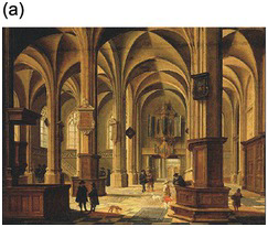
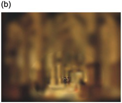
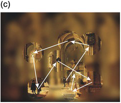
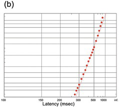
Figure 1.1 (a) On entering an unfamiliar space, we seem to see it all at once. But this is an illusion, for we know that only the central foveal region actually transmits information to the brain with sufficient acuity; what actually happens is that we rapidly scan the area with a series of saccades (b), piecing together this foveal information into a seamless whole (c).
The illusion of universal clear vision comes about because the eye jumps rapidly from one place to another within the scene, getting information about detail that is then stored and forms the basis of our perception (Figure 1.1). These jumps are called saccades (from a French word meaning ‘jerks’) and are examples of gaze-shifting movements. As William Porterfield wrote in 1737 (Porterfield Reference Porterfield1737), ‘… in viewing any large Body, we are ready to imagine we see at the same Time all its Parts equally distinct and clear: But this is a vulgar Error, and we are led into it from the quick and almost continual Motion of the Eye, whereby it is successively directed towards all the Parts of the Object in an Instant of Time.’ Figure 1.2 shows sequences of saccades made by two different subjects viewing a detailed scene suddenly presented to them. You can see that there is a tendency for the saccades to concentrate on the more interesting parts of the scene, those most likely to provide information and requiring detailed visual analysis: blank areas such as sky are on the whole left alone.
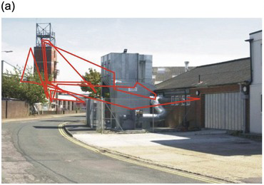
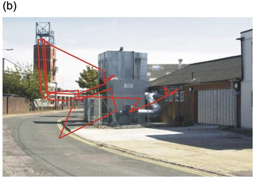
Figure 1.2 Saccadic trajectories (in red, a,b) made by two different subjects viewing the same scene on a computer monitor (courtesy of Dr Benjamin Tatler).
A great deal can be learned from spontaneous saccades of this kind, in particular about the mechanisms that determine what is most likely to be chosen as a target. But as so often in behavioural science, there is a kind of tension between the desire to investigate situations that are ‘ecological’ – as natural and realistic as possible, with the minimum of instructions to the subject as to what they are supposed to do – and the benefits of a controlled laboratory environment with highly constrained tasks and simple, abstract targets. The former are more ‘real’, but generate messy data; the latter can produce precise quantitative results that lend themselves to exact modelling. But they tell us only about a very artificial situation.
The findings that form the subject of this book have come almost entirely from experiments of the second kind, from evoked saccades rather than from spontaneous ones; though they are applicable to more natural situations as well, as we shall see in Section 4.8.
1.1.1 The Step Task
The simplest of all these evoked tasks is the step task. A subject is presented with a small, central visual target and asked to look at it and follow it with their gaze if it moves. A single trial might begin with the target presented centrally, and then – after a delay – jumping either to the left or to the right (Figure 1.3). Both the direction and the delay need to be randomised on each trial, because – as we shall see in Section 3.4 – the saccadic system is extremely intelligent, quickly adapting its behaviour in response to any aspect of the protocol that is predictable (Figure 1.4).
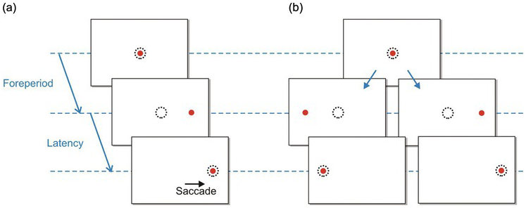
Figure 1.3 A saccadic protocol: the step task. (a) The target (red) is fixated (the dotted circle shows eye position); then after a foreperiod of random duration, it jumps to one side, followed by a saccade as the eye tracks it. The time between target and eye movement is the reaction time or latency. (b) A fully balanced task: after the foreperiod, the target may jump to left or right, at random.
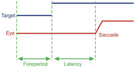
Figure 1.4 The timing of events in a typical step trial. After the foreperiod, the target jumps to one side; then after the reaction time or latency, the eye makes a saccade to the target. The experimenter will normally arrange for the foreperiod to vary randomly from trial to trial, as well as the direction of the target jump.
Figure 1.5 shows the outcome of one such trial. In response to the step movement of the target, the eye moves precisely and extremely rapidly from its initial central location to its new position, in this case a movement of 5 degrees (deg). Saccades such as these are some of the fastest movements the body makes: in this case, the movement is over in about 30 milliseconds (ms), and the peak velocity of the eye in large saccades can be many hundreds of degrees per second. These speeds have evolved because the visual system is effectively blind during a saccade, so the shorter they last, the better (Dodge Reference Dodge1900, Reference Dodge1905).

But this record also demonstrates something very strange indeed. A saccade is a masterpiece of biological engineering, throwing the gaze neatly on to a visual target by a carefully programmed pattern of acceleration and deceleration that can last as little as 20–30 ms, at speeds of up to 800 deg/second (s) (Dodge and Cline Reference Dodge and Cline1901). Yet in another sense, saccades are surprisingly slow: saccadic latency is almost an order of magnitude longer than this, at around 200 ms.
An analogy may make it clearer just how bizarre this is. A fire station receives an urgent message: the Town Hall is on fire! Yet for an hour nothing seems to happen. Then suddenly the fire station doors are flung open, an engine emerges at top speed and arrives at the fire within a minute.
Why does it take nearly 200 ms after the target has been presented for the eye to start to move at all? Why has the evolutionary pressure to make the duration short not been matched by equal pressure to reduce the extreme slowness of the reaction time? This paradox is what this book is all about.
1.2 Procrastination
One of the lines of experimental investigation most diligently followed of late years is that of the ascertainment of the time occupied by nervous events. Helmholtz led off by discovering the rapidity of the current in the sciatic nerve of the frog. But the methods he used were soon applied to the sensory nerves and the centres, and the results caused much popular scientific admiration when described as measurements of the ‘velocity of thought’.
Of course, many physical and physiological processes have to happen, one after another, to allow the eye to move to a visual stimulus. Are these components long enough to explain those 200 ms? A physiologist would immediately think of all the neural events that necessarily cause delay between a stimulus and a response. Every synapse between one neuron and the next introduces a small delay, as do the visual receptors of the eye, and the muscle fibres that eventually move it. And we also need to think about how fast the nerve fibres themselves are. We are used to wires that carry messages at around the speed of light, and computers whose rapidity is measured in nanoseconds; but even in the very fastest nerves the impulses or action potentials that carry information travel at a modest 100 m/s.
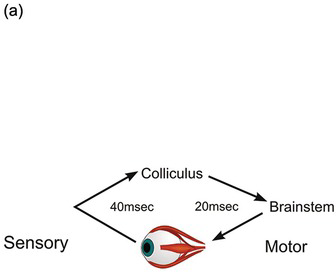
On the other hand, the distances are short: in this case, the most direct route linking the optic nerve to the eye muscles goes through a structure at the back of the brainstem called the superior colliculus (Crosby and Henderson Reference Crosby and Henderson1948), and cannot be much more than some 10 centimetres (cm) (Figure 1.6). So even at 10 meters (m)/s this conduction time can’t be more than 10 ms. Then there is the synaptic delay of 1 ms or so every time information passes from one neuron to the next; the collicular route involves perhaps 10 synapses at most, from retinal receptor to muscle fibre, adding a further 10 ms. The retinal receptors are themselves quite slow to respond to light, so this might account for perhaps 30 ms; and we need to add on perhaps 10 ms for muscle activation and tension development. In all, then, perhaps 60 ms: not negligible, but only about a third of the delay actually observed. In fact, it is not difficult to confirm these estimates directly. If we stimulate the colliculus of a monkey electrically, realistic saccades are produced, with a delay of about 20 ms (Robinson Reference Robinson1972); it is also possible to record collicular responses to visual stimulation, for which the delay is about 40 ms (Wurtz and Albano Reference Wurtz and Albano1980). So our rather crude estimate turns out to be about right.

Figure 1.6 Midline section of human brain, showing the position of the superior colliculus in relation to the eye, and the oculomotor neurons in the brainstem that drive the eye muscles.
So why are saccadic latencies very much longer than simple considerations of conduction and transduction times would lead us to expect? The fundamental reason is that the colliculus is not very intelligent. It is both a sensory and motor structure: recording electrical responses evoked by small stimuli at different visual locations reveals that it maintains a systematic map of the visual world (Cynader and Berman Reference Cynader and Berman1972). Conversely, electrical stimulation at different locations on the superior collicular surface evokes saccades directed in a systematic way to corresponding points on this map (Robinson Reference Robinson1972). So here is an efficient neural device that translates the positions of visual targets into saccades that land on them: exactly what is needed to generate eye movements to look at objects presented at different locations. If the world consisted of single, localised targets in a darkened room, it would function beautifully. But it would be unable to cope even with two stimuli, let alone the huge number of interesting objects out there in the real visual world at any moment.
Worse, it lacks the kind of information it would need to decide which stimuli are actually worth looking at. The function of the superior collicular visual cells is limited essentially to determining where a target is: they have no idea what they are. Left to itself, and in conjunction with other subcortical areas such as the cerebellum, it has all the neural machinery needed to detect the position of a visual object and trigger an appropriately directed movement from the brainstem. But the real world is full of objects, some nice, some nasty, some familiar and safe, some demanding our immediate attention. The superior colliculus is incapable of choosing between them for the very good reason that its neurons have no idea what they are looking at: they respond directly neither to form nor to colour: clearly, they cannot be allowed to determine what we see. This requires much more complex analysis, to which the cerebral cortex in particular seems to be well suited. This kind of processing is more time-consuming than simple mapping. So while these more sophisticated judgements are being made, these higher, cortical, levels must tonically suppress the colliculus, preventing it from making over-fast, simple-minded responses (Figure 1.7).
(a) The simple direct route through the colliculus that carries information about location but not much else.
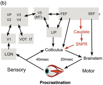
(b) Ascending pathways involving the lateral geniculate nucleus and a variety of cortical areas estimate whether a target is worth looking at. There is tonic descending inhibition, partly via structures in the basal ganglia that normally prevent the colliculus from making fast but erroneous saccades, which is then lifted locally to allow the colliculus to make a more thoughtfully directed saccade. LGN, lateral geniculate; V1, V2, V3, V4, V5, visual cortical areas; LIP, lateral inferior parietal area; FEF, frontal eye field; SEF, supplementary eye field, VP, ventral posterior area; MT, middle temporal area; VOT, ventral occipitotemporal cortex; IT, inferior temporal cortex.
Figure 1.7 Highly schematic diagrams of direct and indirect pathways by which visual information could trigger a saccade.
Figure 1.7(a) shows this older and simpler visual pathway through the colliculus. But a huge amount of visual information takes a quite different route. Via a thalamic nucleus, the lateral geniculate (LGN), this information projects to visual cortical area V1 (striate cortex), and thence, directly or indirectly, to many other cortical areas responsible for analysing the attributes – colour, form and motion – of the retinal image (Figure 1.7(b)). These in turn project both to areas that are not wholly visual, such as the lateral inferior parietal area (LIP), and to areas that are specifically oculomotor, the frontal and supplementary eye fields (FEF and SEF). So there are many routes by which all these areas influence the superior colliculus and the areas of the brainstem concerned with controlling saccades. Many of them are tonically inhibitory, that is, their default is to inhibit saccade initiation. Corresponding to this continuing suppression, there are many inhibitory pathways that descend from cortex, such as the basal ganglia, that fire continuously, often at a very high rate, until the cortex has finished working out what movement to make next. This blanket of inhibition is lifted in a single localised area (Figure 1.8(a)), permitting the superior colliculus to carry out its basic function of converting visual location into an appropriately directed eye movement (Hikosaka and Wurtz Reference Hikosaka and Wurtz1983a, Reference Hikosaka and Wurtz1983b, Reference Hikosaka and Wurtz1983c, Reference Hikosaka and Wurtz1983d, Wurtz and Goldberg Reference Wurtz and Goldberg1989, Hikosaka, Takikawa et al. Reference Hikosaka, Takikawa and Kawagoe2000). In a sense, they can be thought of as preventing the collicular route from operating, so that reaction times are longer than they might otherwise be.
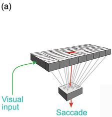
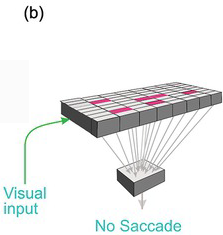
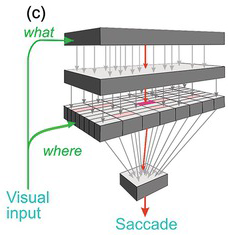
Figure 1.8 (a) The superior colliculus copes well if there is only one target, but not if there are many of them (b). Descending tonic inhibition is then needed (c), which is locally lifted when the decision has been made.
In other words, latency is mainly due not to conduction along nerves and across synapses, or the time taken to activate receptors and muscles (as is obvious from a second mysterious property mentioned earlier, the strangely random variability of latency: see Sections 1.3 and 5.3), but a deliberate mechanism of procrastination. A possible early response is suppressed in order to decide more carefully on a later one. Because of this procrastination, latency is in effect telling us how long it takes the higher levels to decide what to look at. So what latency represents is the time needed to work out which of all the possible things we might do is best. Reaction time is decision time.
1.3 Analysing the Variability of Reaction Time
When you can measure what you are speaking about, and express it in numbers, you know something about it; but when you cannot measure it, when you cannot express it in numbers, your knowledge is of a meagre and unsatisfactory kind.
When Nature does something odd, it is often a sign of a vulnerability asking to be scientifically exploited. With modern computer-based equipment, it is possible to obtain very large data sets of saccadic latency measurements and determine rather precisely the form of this random variability, as a first step to trying to understand why it happens.
It turns out that random reaction times obey a relatively simple law that applies not just to saccades to visual targets, but also to all kinds of responses, to a wide variety of stimuli, and in a remarkably similar way throughout the animal kingdom, from frogs to humans. A natural first step is to look at the distribution of variability across different trials in an experimental run, in the hope we can characterise the type of stochastic process that may be giving rise to it. Curiously enough, although some of the earliest experimenters were very well aware of the importance of doing this (Yerkes Reference Yerkes1904), in general it has been rare for those who have measured reaction times to bother to publish more than means or medians of their data. Perhaps as a consequence, while many have developed more or less elaborate theories to relate average reaction times to stimulus or response parameters, rather few have been equally concerned with the distribution of the reaction times themselves (Noorani and Carpenter Reference Noorani and Carpenter2011, Antoniades and Carpenter Reference Antoniades and Carpenter2012, Carpenter Reference Carpenter and Reddi2012). Of those who have, some have used them in half-hearted tests of models arrived at on theoretical grounds: some examples are presented in Appendix 1. Even Luce’s masterly analysis (Luce Reference Luce1986) of a wide range of models for reaction times devotes relatively little space to the critical evaluation of such models against existing distributional data. It almost begs belief that in so many experiments, particularly in the clinical arena, this information is simply thrown away (Antoniades and Carpenter Reference Antoniades and Carpenter2012, Carpenter Reference Carpenter and Reddi2012).
The particular reaction time distribution that forms the focus of this book arose not theoretically but empirically, as the result of a search for some way of summarising large amounts of data from saccadic latencies. It was only subsequently that a very simple functional explanation for its existence was proposed (Carpenter Reference Carpenter, Fisher, Monty and Senders1981). The discovery that the same model seemed to underlie very many kinds of reaction time tasks, and provided a remarkably good fit to previously published distribution data from both early and recent sources, came relatively late. Thus, whereas the traditional approach has generally been to devise a good theory and only then (perhaps) see if it works, the novelty here was to start with an empirical description and find a theory for it later. Since the model has very few parameters and the theory is a simple one, the approach does not seem entirely unjustified. In the circumstances, it would be surprising if the nature of this distribution had never occurred to anyone before. Yet apart from a passing mention by Jenkins (Reference Jenkins1926) in a list of theoretical possibilities (if indeed that is what he meant by a ‘harmonic’ distribution), this appears to be the case.
1.3.1 Kinds of Histograms
The conventional way of presenting data about stochastic distributions is the frequency histogram. We start by dividing the range of possible data values into a series of ‘bins’ (or categories), usually of equal width. For reaction times, which usually range from a few tens to several hundred milliseconds, 10 ms is quite a convenient choice of bin-width. We then take each of our data values and assign it to a corresponding bin, keeping a tally of how many end up in each one. The result is then typically plotted as a bar chart (Figure 1.9).
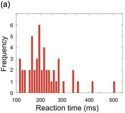
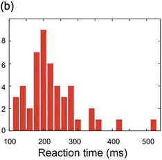
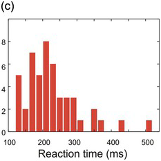
Figure 1.9 The arbitrariness of frequency histograms. The same data set (N = 50) is plotted first with 10 ms bins (a), then with 20 ms bins (b), and finally (c) with the 20 ms bins shifted by 10 ms.
Histograms of this kind are familiar and intuitive, but suffer from a number of grave defects: from a mathematical point of view, they are thoroughly unsatisfactory. Unless the data set is extremely large, they have randomly bumpy profiles that can give rise to spurious conclusions about the form of the data. Furthermore, the position and size of these bumps depend on what bin-width one happens to have chosen and where their boundaries are (Figure 1.9). In addition, the Y-axis of a frequency histogram is arbitrary: it too depends both on the width of the bins and on the total number of data points, making it difficult to make a visual comparison between one set of data and another. Finally, it is not easy to present several different frequency histograms in the same chart, so they are wasteful of space.
Fortunately, there is another way of plotting distributional data that solves all of these problems: the cumulative histogram. Here, instead of asking ‘How many data points lie between 200 and 210 ms? How many between 210 and 220?’ and so on, we ask a simpler question: ‘How many are less than 210 ms? How many less than 220?’ The result (Figure 1.10) is a curve that necessarily increases to the right, and is normalised in the sense that it must start at zero (there will always be some x value smaller than any of the data) and finish at 100% (since there must similarly be an x value that is bigger than all the data). If we choose to plot percentages rather than raw numbers, then this cumulative histogram is automatically normalised. Bin-width no longer has any effect on the overall shape; it simply alters the resolution, so that the arbitrariness of the appearance of the frequency histogram is avoided. Finally, we can have several cumulative histograms on one chart without confusion (Figure 1.11).
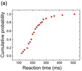
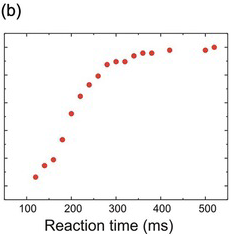
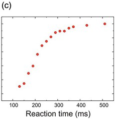
Figure 1.10 The same histograms as shown in Figure 1.9, but plotted cumulatively (a,b,c): their shapes are essentially unaffected by bin size or displacement.

One kind of distribution that crops up again and again in scientific work is the Gaussian or Normal distribution (Gauss Reference Gauss1809) – popularly known as the ‘bell curve’. It is the most fundamental of all random distributions, since mathematically it results from any situation in which a very large number of independent random events – which need not themselves be Gaussian – add together in a linear fashion. It is not surprising that much biological variation is Gaussian, since it results from the summation of a multiplicity of tiny genetic and environmental factors. Plotted as a conventional frequency distribution, it is indeed bell-shaped (Figure 1.12). To specify its shape, we need only two parameters: the mean (μ) and the standard deviation (σ). Often it is convenient to refer to the variance, σ2.
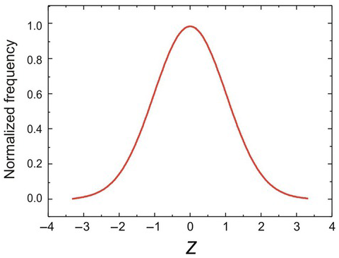
Figure 1.12 Gaussian frequency function, normalised to have a value of 1 at the mean, μ (in this case, zero). The horizontal Z scale (X-axis) shows deviations of x from the mean, in units of σ: so Z = 2 means that x is two standard deviations from the mean.
If we are applying this to frequency distributions, it can also be referred to as the probability density function or PDF, P(Z). The formula for P is given in Appendix 1, App 1.2. Corresponding to the PDF is its integral, the cumulative distribution function or CDF, C(Z), whose formula is also given in Appendix 1, App 1.2. It is S-shaped (Figure 1.13) and is normalised in the sense that it ranges from 0 to 1.
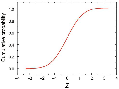
Figure 1.13 The same Gaussian function as in Figure 1.11, plotted cumulatively as the CDF, C(Z).
Finally, there is a clever trick for seeing immediately whether a given distribution is or is not normal, which is not as well known generally as it ought to be. It is to plot a histogram using not a linear scale for the cumulative probability, but a distorted one (rather like log-paper) that is stretched out at both low and high probabilities in such a way as to turn the S-shaped distribution into a straight line. More specifically, this is a probit or ‘probability’ scale, that simply embodies the inverse of equation (2) above; distances Z along it can be thought of in units of one standard deviation, with zero in the middle (corresponding to the mean or median, C = 50%; thus, Z = 1 corresponds to 1 standard deviation (SD) from the mean, or P = 84.1%; Z = 2 is the same as P = 97.7%, and so on).
If the distribution in question is indeed Gaussian, its parameters can be derived directly from this straight line. The mean (and median) is the value of x where the line cuts the horizontal line at C = 0.5; the slope of the line is inversely related to σ (Figure 1.14). More exactly, σ is given by the horizontal distance between where the line intercepts C = 0.5 and where it intercepts Z = 1.

1.4 The Recinormal Distribution
Now conventional histograms of reaction times are not Gaussian, or even symmetrical. They have a long tail that extends further in the direction of long reaction times than short. This is a nuisance: the distribution does not fit any of the more standard mathematical distributions (Gaussian, Poisson, Gamma, etc.) particularly well. A lot of fruitless effort culminated finally in the realisation that the lack of success was simply an indication that one was thinking about the problem the wrong way.
Because we measure reaction times using clocks or their computer equivalents, which tick away in a linear fashion, it is natural to assume that the time taken to respond is a fundamental variable. But if we ask, instead, not about how the response is measured but how it is generated, we come to a completely different conclusion. Think, for instance, of a process initiated by the stimulus and proceeding at a certain rate until some criterion is reached that completes the decision and initiates a response. If there is variability in the time that is taken, isn’t the simplest explanation that the rate at which the process occurs is varying? This is what we see in chemical reactions, for instance, if we vary the temperature. So instead of looking at reaction times (T), we should be looking at reaction rates: we should be analysing not T, but 1/T, the reciprocal of the reaction time, or promptness.
Suppose, then, we create a conventional histogram not of reaction time but of promptness. We could do this with a computer, but in some ways it’s more fun to use a graphical technique that lets us see what is going on more directly. The trick is to use a special scale – a reciprocal scale – that transforms distances into their reciprocals, just as the more familiar log scale does for logarithms. To aid interpretation, longer times are still to the right, and it’s convenient to have our ‘origin’ (actually equivalent to infinity, since 1/T is then zero) to the right. Here’s the result (Figure 1.15). Magically, we suddenly find that the asymmetry that is such an awkward feature of conventional plots has disappeared – indeed, the histogram looks Gaussian. This not only makes for easier mathematical analysis, but also suggests that we have reached a genuinely fundamental phenomenon.
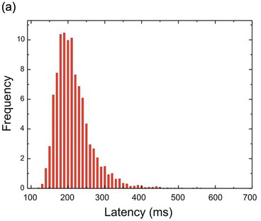
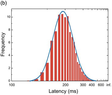
Figure 1.15 A simulated set of 5000 latencies (μ = 5, σ = 1) plotted as a conventional frequency histogram (a), showing the obvious skewness of the distribution. (b) The same data plotted using a reciprocal sale for latency: note that for convenience the latencies still increase to the right. The distribution is now relatively symmetrical, and indeed very similar to a Gaussian (blue).
1.4.1 Reciprobit Plots
A convenient way to see at once whether reciprocal latency really is Gaussian is to use the trick described earlier (Section 1.3.1), of plotting latency as a cumulative histogram on a reciprocal scale. Then we repeat our trick of using a specially distorted scale, but this time on the vertical probability axis. This is a probit scale, specifically designed to stretch out the tails of the distribution in such a way that if the distribution is indeed Gaussian, we should get a straight line. Because it combines a reciprocal and a probit scale, we can call it a reciprobit plot. A Gaussian distribution of promptness should then give a straight line (Figure 1.16). The line intercepts the right-hand axis (t = infinity) at Z = k, given by μ/σ. It is also convenient to call the associated distribution a recinormal distribution. With certain reservations (Section 2.2), distributions of reaction times – not just for saccades but for other kinds of response as well – do indeed turn out to be recinormal.
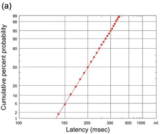
(a) The same data as in Figure 1.15, but plotted cumulatively using a probit scale. This systematically stretches the ends of the ordinate axis in such a way that if the data are indeed Gaussian, it generates a straight line. Since the latency uses a reciprocal scale, this is a reciprobit plot.
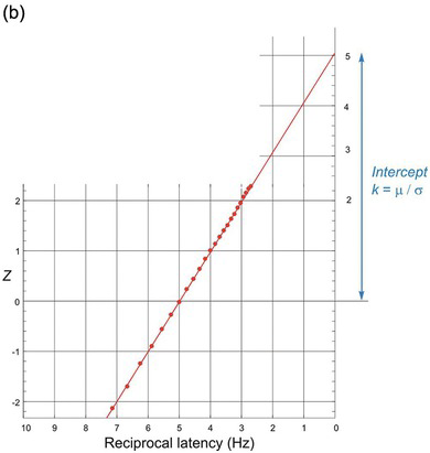
(b) The same cumulative plot with the latency scale now explicitly of reciprocal latency (1/T), increasing leftwards to facilitate comparison; the probability scale uses units of Z. The data can be extrapolated to an intercept on the right-hand axis (T = infinity or 1/T = 0), whose value is μ/σ (in this case, 5) in Z units.
On a reciprobit plot, the distribution cuts the horizontal 50% axis at the median: this is also the mean, since the distribution is Gaussian. Note that the intercept k represents a probability: that the linear approach to threshold ergodic rate (LATER) signal will never reach its threshold at all, in other words, that r < 0. Under most conditions, this probability is vanishingly small, but if we reduce the amount of available information, for instance by making discrimination increasingly difficult, this probability can be measured (see Section 4.7.2).
In Chapter 3, we introduce a simple model of a decision process that would give rise to such a distribution. Meanwhile, we need to separate clearly the purely empirical question of whether in fact real reaction times do or do not conform to a recinormal distribution, and what we can deduce about the underlying mechanisms if it turns out that they do. But quite apart from the validity of any particular explanatory model, if it is true that sets of reaction times can be adequately described with only two parameters, this in itself has great practical importance, particularly in clinical studies (see Appendix 2).
1.4.2 A Gallery of Reciprobits
This observation on reaction times was originally discovered through analysis of saccadic data from our own laboratory. But to form some idea of its general applicability it seemed to us that a fairer and stricter test was to re-examine previously published data about latency distributions in as wide a range of situations as possible, and see whether they behaved the same way. What follows is a gallery of older data – published over the past hundred years or more – replotted as reciprobit plots. Kolmogorov–Smirnov (Kolmogorov Reference Kolmogorov1941, Smirnov Reference Smart, Flew and MacIntyre1948) one-sample statistical tests are used to test conformity with a recinormal distribution, and none is significantly different (p > 0.05).
Figures 1.17–1.26 show reciprobit plots of 56 data sets taken from a wide cross section of the earlier published literature, covering a variety of types of response, of stimuli and of species. They are certainly not exhaustive; apart from omissions through ignorance, examples where the number of trials was too small (in general, fewer than 50) have been excluded, as have instances where the conditions of the experiment were insufficiently clearly described to be sure what it was that was being measured, or where data sets were needlessly repetitive. There is no wholly satisfactory way of arranging them: we start with the relatively simple and finish with some more complex examples, and some that are frankly bizarre.

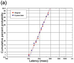
(a) Two different runs of around 100 trials at an interval of 6 years (R. H. S. Carpenter, unpublished data);

(b) Different amplitudes, 120 trials per data set (White, Eason et al. Reference White, Eason and Bartlett1962);
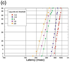
(c) Different target luminances, expressed in log units relative to foveal threshold, 100 trials per data set (Wheeless, Cohen et al. Reference Wheeless, Cohen and Boynton1967);
Figure 1.18 Reciprobit plots of human saccadic latencies to step targets.
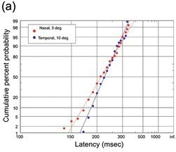
(a) Monkey, nasal saccades with an amplitude of 5 deg (123 trials) and temporal saccades of 10 deg (89 trials); a K-S test shows that the difference between the plots is not statistically significant (Fuchs Reference Fuchs1967).
(b) Cat saccades, 95 trials, showing an early component (Evinger and Fuchs Reference Evinger and Fuchs1978).
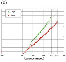
(c) Cat nose-poke responses, for trials with large and small rewards (Avila and Lin Reference Avila and Lin2014).
Figure 1.19 Other species.
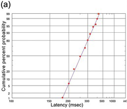
(a) From Walsh (Reference Walsh1952); N = 286).
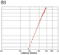
(b) A large data set (N = 825) from a careful observer (Welford Reference Welford1959).
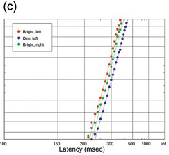
(c) From Johnson (Reference Johnson1918), comparing left and right hands, and bright and dim stimuli; because of the large size of the data sets (ca. 900 trials each), the small difference between the left and right hands is in fact statistically significant (K-S test). Note that manual responses are in general slower than saccadic, and tend to lack early components.
Figure 1.20 Manual human responses to visual stimuli.

(a) To visual stimuli (Schupp and Schlier Reference Schupp and Schlier1972), instructive in that its statistical fit (p = 0.91, K-S test; N = 546) is much better than might be expected from its appearance, showing the importance of data points near the median as opposed to the tails.
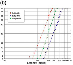
(b) Auditory, from three of Wells’ subjects, D (194 trials), W (95) and Wh (196), two with a slight hint of an early component (Wells Reference Wells1913).
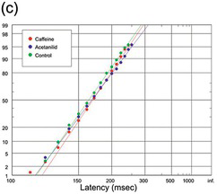
(c) Visual, from Schilling 1921, #3770, comparing the effects of two pharmacological substances, caffeine and acetanilide, with a control; in fact, the plots are not significantly different from one another (K-S test) despite the large data sets (800 trials each).
Figure 1.21 Manual human responses.
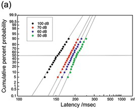
(a) Human: 4 different intensities, 100 trials each (McGill and Gibbon Reference McGill and Gibbon1965).
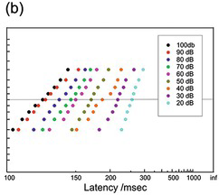
(b) Human, 9 different intensities, 60 trials each (McGill Reference McGill, Luce, Bush and Galanter1963).
(c) Cat manual responses (389 trials) to an auditory stimulus (Schmied, Benita et al. Reference Schmied, Benita, Conde and Dormont1979).
Figure 1.22 Manual reaction times to auditory stimuli of different intensities.
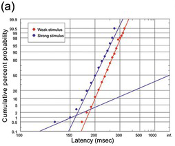
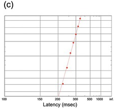
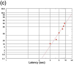
(a) Two of Kiesow’s (Kiesow Reference Kiesow1904) sets of reaction times to tactile stimuli of various strengths (N = 200), with a hint of an early component with the strong stimulus.
(b) Frog reaction time to touch (Yerkes Reference Yerkes1904).
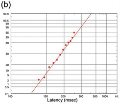
(c) The very long jellyfish reaction time to light, but a very small data set (N = 10): as a result, it is ragged, though not significantly different from recinormal (K-S test) (Yerkes Reference Yerkes1903).
Figure 1.23 Some of the earliest distributions to be published.
(a) Manual auditory, 4436 trials (Green and Luce Reference Green and Luce1971).
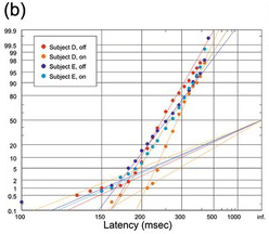
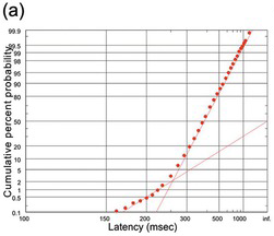
(b) Manual, two subjects, to illumination or extinction of visual target, 400 trials each (Jenkins Reference Jenkins1926).
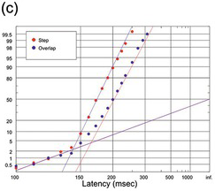
(c) Saccadic, in step (red, 1875 trials) and overlap (blue, 998) tasks (Carpenter Reference Carpenter, Fuchs, Brandt, Büttner and Zee1994).
Figure 1.24 Human reaction times with prominent early components.
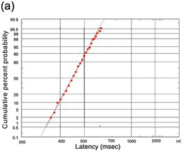
(a) In a task in which the subject had to decide whether the majority of a set of lines was inclined to the left or right (kind permission of Dr Ben Pearson).
(b) Subjects decided whether a suddenly presented picture did or did not have an animal in it; note that this is combined data from 9 subjects (Thorpe, Fize et al. Reference Thorpe, Fize and Marlot1996).
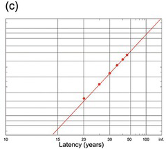
(c) A very long decision: age at first marriage for UK males in 2005 (web data, UK Home Office).
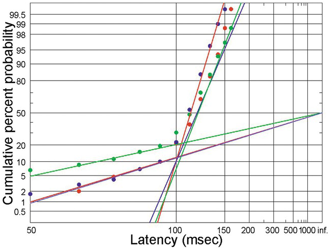
Figure 1.26 Initiation of smooth pursuit in response to a target moving off at constant velocity; 3 subjects, 300 trials each (Merrison and Carpenter Reference Merrison and Carpenter1995) showing prominent early responses.
When comparing these plots, it is important to bear in mind two points.
The first is that because of the probit scale, in general these plots hugely exaggerate the extreme tails of the distribution. So the scatter which is the inevitable effect of random variation from trial to trial is very much more apparent at the two ends of the distribution than it is in the middle. In a large data set with a thousand measurements, the points in the region of 0.1% or 99.9% are derived from just one or two individual trials, and their exact position is consequently of little significance. As a result, we shall sometimes see that a distribution that fits a straight line very well in the centre may show quite substantial deviations at the ends despite being statistically perfectly acceptable. So distributions that are in fact absolutely compatible with a recinormal distribution may look poor to the unpractised eye because of a very small number of aberrant trials: the points at the extremes may only represent one or two individual trials: it is the points in the middle of the distribution that contribute most to goodness of fit.
Second, one must be aware of the overwhelming effect of the size N of a data set on the scatter of the points. With small data sets of a hundred or so, the apparent scatter will look much poorer than what is seen when N is a thousand or more (Figure 1.17), yet both may give equally good fits.
Finally, although most of the plots illustrate data sets for which essentially the entire population appears to conform to a recinormal distribution, in some there are examples of cases where there appears to be a small sub-population of unusually fast responses. In general, these early responses tend to lie along a different straight line that goes through what is in effect the origin of these reciprobit plots, namely, the intercept (t = infinity, C = 50%). They are considered in more detail in Section 2.2
We start with human saccadic responses to visual targets. Figure 1.18(a) gives an idea of how robust these distributions are over time. Though a little ragged because of the small N, the two runs happened to be made by the same subject with identical stimuli and conditions on two occasions separated by six years, and the two distributions are not statistically distinguishable (Kolmogorov–Smirnov (K-S) test (Kolmogorov Reference Kolmogorov1941, Smirnov Reference Smart, Flew and MacIntyre1948)), giving some idea of the kind of stability that saccadic latencies can show under controlled conditions. Figure 18(b) and (c) show older data for saccades in a step task with variation of the eccentricity of the target (White, Eason et al. Reference White, Eason and Bartlett1962), or its luminance (Wheeless, Cohen et al. Reference Wheeless, Cohen and Boynton1967). Despite the variation in the stimulus conditions (which in the latter case produce a variation in median latency by more than a factor of two), each data set conforms to the recinormal distribution. Changes in eccentricity appear to alter μ but leave k relatively unchanged, while target luminance seems to influence both.
Figure 1.19 shows responses in some other species: monkey, cat (with prominent early responses) together with nose-poke latencies in the rat.
Figures 1.20 and 1.21 show manual human responses mostly to visual stimuli, some with large data sets that demonstrate the extent to which in such cases the accuracy of the recinormality extends far into the tails of the distributions. They also include examples of experimental manipulation, for instance, by pharmacological substances.
Figure 1.22 shows manual responses to auditory stimuli. These data (McGill Reference McGill, Luce, Bush and Galanter1963, McGill and Gibbon Reference McGill and Gibbon1965) have frequently been reproduced for the purpose of testing theories of reaction-time distribution, perhaps because they are both remarkably regular, considering their very small values of N. In both cases, the effect of reducing the stimulus intensity is to lengthen reaction times, the curves tending to swivel round a fixed value of k rather than simply being displaced to the right in a parallel fashion. One of the sets (40 decibels (dB)) is oddly bent, but otherwise the fits are very good.
Finally, some extremely early data sets, dating from over a century ago (Figure 1.23). The Kiesow data are interesting (Figure 1.23(a)) in that they use a tactile stimulus, and also clearly demonstrate an effect of changing the strength of the stimulus. Figure 1.23(b) is also tactile, in a frog: it is ragged because of the small number of observations, but statistically compatible with a recinormal, as is the final even smaller data set (Figure 1.23(c)) showing the (very slow) responses of a jellyfish to light.
A graphical procedure like the reciprobit plot can often provide more insight than blind number-crunching. For instance, if you look critically at the Kiesow data, though the great majority of the blue data points lie satisfactorily on the expected straight line, the very earliest data point is much too high – there are more early responses than the law would predict. When we look at very large data sets (for example, Figure 1.23(a)), especially under conditions where the target is highly expected or the subject is trying as hard as possible to be fast, it is clear that there is indeed a separate sub-population of faster responses that lie on a different line, intersecting the main one but of shallower slope and extrapolating to the origin (the point corresponding to infinity and p = 0.5). Although these early responses look prominent on a reciprobit plot, they typically form only a small proportion of the population (some 2–5%) and therefore do not normally have a significant effect on the goodness of fit of the population as a whole (Section 2.2).
Figure 1.24 shows examples of distributions in which an early sub-population is more marked, though in no case do they form more than 2% of the total. Figure 1.24(a), of manual responses to an auditory stimulus (Green and Luce Reference Green and Luce1971), is a very large data set indeed (N = 4436); as a result, the shape of both the main population and the sub-population is particularly sharply defined. This is followed by plots of manual responses by two subjects to the illumination or extinction of a visual target (Figure 1.24(b)), with prominent early sub-populations, and finally human saccadic responses in a step and in an overlap task (Carpenter Reference Carpenter, Fuchs, Brandt, Büttner and Zee1994) (Figure 1.24(c)), where the large value of n again results in a clear definition of the early sub-population. In each case, these early responses seem to lie on a straight line of much shallower slope than the main distribution that passes through C = 50% at t = ∞ (in other words, μ = 0 and therefore k = 0). A model for these early responses is presented in Section 2.2.
1.4.3 But Are Saccades the Result of a Decision?
When we move our eyes to a suddenly presented target, is it reasonable to call it a decision? In ordinary parlance, we tend to use ‘decision’ to describe much more protracted processes: deciding to get out of bed, deciding what to have for breakfast, deciding where to go on holiday. Even pressing a button when a light comes on requires so little thought that it hardly seems appropriate to call it a decision at all, let alone the almost reflex response with which we flick our eyes on to a sudden visual target. But when we examine the form of the distributions of reaction times for different kinds of tasks – those that most people would consider reflexive, and those they would consider voluntary and therefore genuine ‘decisions’ – we find the identical, recinormal form for all of them. Figure 1.25 shows some examples. We see reciprobit plots for a difficult task in which the subject was presented with a set of lines of different orientations, and had to decide whether the majority were pointing in one direction rather than another (Figure 1.25(a)). The demanding nature of the task is reflected in the long mean reaction time (some 450 ms), but the form of the distribution is the same straight line that is seen in a saccadic step task. Figure 1.25(b) shows a large data set from (Thorpe, Fize et al. Reference Thorpe, Fize and Marlot1996) of the distribution of response times in a task that by any standards must be regarded as a ‘decision’: subjects had to respond to a picture of a complex scene by identifying whether or not it contained an animal. Because of the difficulty of the decision, the median reaction time is much longer; but – despite the degrading effect of combining data from several subjects – the recinormal law is still followed.
Finally, a very long decision indeed: Figure 1.25(c) shows the age at first marriage in the UK, and – very surprisingly – it follows the same recinormal distribution extremely well, despite the huge size (N = 170,890!) of the data set. Obviously, it is highly unlikely that this is due to the same neural mechanism giving rise to button-pushes and saccades, but the common principle is a process that reaches completion at a rate that is subject to Gaussian random variability which still applies.
1.4.4 Smooth Pursuit
We have seen that a visual target that suddenly appears, or jumps to a new position, typically evokes a saccade to fixate it. But when a target moves relatively smoothly and slowly, a completely different kind of eye movement is generated, called smooth pursuit (Rashbass Reference Rashbass1961, Robinson, Gordon et al. Reference Robinson, Gordon and Gordon1986, Missal and Keller Reference Missal and Keller2002, Thier and Ilg Reference Thier and Ilg2005). Whereas the function of the saccade is to capture a new target by moving it on to the fovea, smooth pursuit is intended to hold it there despite its movement. Like saccades, smooth pursuit is controlled by a sophisticated and intelligent system that does its best to anticipate how the target is going to move. As a result, the performance of a subject tracking a target that moves repetitively back and forth tends to get better and better as time goes on and the brain is able to predict the motion. Figure 1.26 shows latencies of smooth pursuit by three subjects to a target suddenly moving off at constant velocity (Merrison and Carpenter Reference Merrison and Carpenter1995). Though these responses have a very short median latency, the general shape conforms very well to the pattern of the previous data sets, but with a much larger (10–20%) proportion of responses in the early sub-population. A saccade is usually made in each trial at about the same time as the smooth pursuit begins, intended to make up for the time lost during the latent period, during which the target has been moving (Rashbass Reference Rashbass1961). It is quite interesting that the latencies of the smooth pursuit and saccadic responses in this situation are usually uncorrelated with each other, suggesting that there are separate units, acting independently, for saccades and smooth pursuit (Merrison and Carpenter Reference Merrison and Carpenter1994).
To summarise, reciprocals of reaction times are in general Gaussian. For data sets that are large enough to provide an adequate comparison, and if we ignore the existence of a small population of early responses, the recinormal distribution provides a better description than any other previously proposed, except in the case of distribution functions where the large number of parameters permits the function to be moulded, in effect, into the same shape as the recinormal (see Appendix 1, App 1.3–1.5). It is also clear that data sets of fewer than a hundred or so observations are of very little help in trying to validate theories of reaction time distributions. Unless a model is hopelessly inadequate, it will differ from other models only in the tails of the distribution: this is why we need large numbers of trials to evaluate one model decisively against another.


