


NOMENCLATURE
- ATON
Autonomous Terrain-based Optical Navigation
- BSM
Binary Shadow Matching
- DLR
The German Aerospace Center
- FoV
Field of View
- GTM
Global Topography Model
- ICP
Iterative Closest Point algorithm
- IMU
Inertial Measurement Unit
- LDB
Landmark Database
- MSE
Mean Squared Error
- NavCam
Navigation Camera
- P3P
Perspective-3-point Problem
- SfM
Structure from Motion
- SHOE
Shadow-Hiding Opposition Effect
- SLAM
Simultaneous Localization and Mapping
- SPL
Synthetic Photometric Landmark
- UKF
Unscented Kalman Filter
- VO
Visual Odometry
Greek symbol $\alpha$
Phase Angle
-
$\mu$
Emittance Angle
-
$\mu_0$
Incidence Angle
-
$\rho$
Scaling Constant
-
$\omega$
Single Scattering Albedo


1.0 INTRODUCTION
Visual navigation, also called vision-based or optical navigation, is an important research topic and of particular interest for future CubeSat missions that will operate close to a distant solar system small body, as they will need to independently position themselves relative to their target.
Navigation methods, in general, can be divided into two classes: absolute and relative. Absolute navigation uses measures (line-of-sight, position, orientation, pose) in either the target- or spacecraft-fixed coordinate frame. Examples of absolute navigation use various landmark- and global map-based methods. In turn, relative navigation exclusively uses measures of change relative to an earlier point in time, e.g. the change in pose since a starting time. Typically, however, they return absolute pose estimates in an arbitrary internal frame or in a frame initialised to coincide with a real-world coordinate frame. Measurement errors will build up over time leading to a growing bias in the absolute pose estimates returned. Relative pose estimation in the visual navigation context is called visual odometry (VO). When integrated with a navigation filter, VO can increase the navigation accuracy significantly by providing constraints from the current state to past states. At least one absolute pose-estimation method is typically needed to limit the error due to the drift inherent in VO.
The work presented here was started as an investigation to determine the visual navigation architecture suitable for a CubeSat mission called APEX(1) (previously ASPECT(Reference Kohout, Näsilä, Tikka, Granvik, Kestilä, Penttilä, Kuhno, Muinonen, Viherkanto and Kallio2)), which is scheduled to be deployed in 2027 near the binary asteroid 65803 Didymos by ESA’s Hera mission(Reference Michel, Kueppers, Sierks, Carnelli, Cheng, Mellab, Granvik, Kestilä, Kohout and Muinonen3). APEX will be deployed at a distance of 10km from Didymos and then navigate to a 4-km circular orbit, where it will stay for several weeks. Next, APEX will navigate to the  $L_4$
and
$L_4$
and  $L_5$
points in the Didymos system, roughly 1200m from the centres of the primary and secondary body, whose mean diameters are around 780 and 135m, respectively(Reference Naidu, Benner, Brozovic, Ostro, Nolan, Margot, Giorgini, Magri, Pravec and Scheirich4). The extended mission plan also includes periods where APEX will stay near the
$L_5$
points in the Didymos system, roughly 1200m from the centres of the primary and secondary body, whose mean diameters are around 780 and 135m, respectively(Reference Naidu, Benner, Brozovic, Ostro, Nolan, Margot, Giorgini, Magri, Pravec and Scheirich4). The extended mission plan also includes periods where APEX will stay near the  $L_1$
and
$L_1$
and  $L_2$
points at a distance of around 180m from the centre of mass of the slightly elongated secondary body. The altitude is expected to be from 70 to 90m during these periods.
$L_2$
points at a distance of around 180m from the centre of mass of the slightly elongated secondary body. The altitude is expected to be from 70 to 90m during these periods.
1.1 Reference mission
Even though our interest is with the APEX mission, the analysis presented in this article uses the Rosetta mission scenario for the comet 67P/Churyumov–Gerasimenko. The reason for this is that no detailed 3D models or images from Didymos were available when this research was performed, while an accurate 3D model(5) and NavCam images(6) are now available from the Rosetta mission. These images also have metadata which give the comet position and Rosetta pose. Although our reference mission is to a comet, we will continue to use the term asteroid, as the use of “small body” would be somewhat unwieldy. Other asteroid parameters such as orbital elements and the rotation period are taken from this comet. The Rosetta NavCam parameters of 5°  $\times$
5° FoV and 1024
$\times$
5° FoV and 1024  $\times$
1024 pixel resolution were used in order to allow testing with actual Rosetta NavCam images.
$\times$
1024 pixel resolution were used in order to allow testing with actual Rosetta NavCam images.
1.2 Past missions and related work
The first asteroid mission which used a form of optical navigation was NASA’s NEAR mission(Reference Owen, Wang, Harch, Bell and Peterson7). Earth-based human analysts had a global topography model (GTM or shape model) of asteroid 433 Eros, which was projected on top of a target NavCam image. The position and orientation of the model were adjusted manually so that the limbs would match. When the probe was too close to the asteroid to have its limbs visible, 3D-ellipses were fitted manually to craters and used as landmarks.
The Rosetta comet mission(Reference de Santayana and Lauer8) and the Dawn asteroid mission(Reference Mastrodemos, Rush, Vaughan and Owen9) used human analysts for shape model estimation and the creation of landmarks. The landmarks consisted of a detailed, textured 3D-model of a small region around a physical landmark like a boulder or crater and were called “L-maps”. Phase correlation was used to match the rendered L-maps in the database to NavCam images. To be able to render the L-maps, a rough relative pose of the spacecraft and asteroid was needed in addition to the direction of sunlight. The previous pose estimate and possibly a phase correlation pass using the rendered asteroid shape model, were used. The same method is currently used by the OSIRIS-REx asteroid mission(Reference Lorenz, Olds, May, Mario, Perry, Palmer and Daly10) to 101955 Bennu, with the difference that landmark matching can be done on-board.
Hayabusa 1(Reference Miso, Hashimoto and Ninomiya11,Reference Hashimoto, Kubota, Kawaguchi, Uo, Shirakawa, Kominato and Morita12) used a combination of asteroid centroids estimated from NavCam images and distance measurements from a laser range finder to position itself in relation to the asteroid 25143 Itokawa while the asteroid could fit in the FoV. When closer than that, the original plan had been to use a template extraction and matching scheme and to measure the distance to the matched areas using the laser range finder. However, this method was never used. Navigation was done manually from the ground instead because one of the reaction wheels had broken down, thus preventing targetted laser measurements. For landing, Hayabusa 1 used a combination of the laser range finder and tracked artificial target markers that it deployed on Itokawa.
Some scale and rotation invariant automatic local feature detectors like SIFT(Reference Lowe13), SURF(Reference Bay, Ess, Tuytelaars and Van Gool14), BRISK(Reference Leutenegger, Chli and Siegwart15) and ORB(Reference Rublee, Rabaud, Konolige and Bradski16) were evaluated by Takeishi et al.(Reference Takeishi, Tanimoto, Yairi, Tsuda, Terui, Ogawa and Mimasu17) for the Hayabusa 2 mission that arrived in June 2018 at the asteroid 162173 Ryugu. However, at the time of writing, no public information seemed to be available about the navigation algorithms used by this mission.
The German Aerospace Center (DLR) has been working since 2010 on a comprehensive optical navigation system called Autonomous Terrain-based Optical Navigation (ATON)(Reference Theil, Ammann, Andert, Franz, Krger, Lehner, Lingenauber, Ldtke, Maass and Paproth18). Their reference mission is to land a probe on the Moon using a sensor set composed of an inertial measurement unit (IMU), star tracker, navigation camera, a laser altimeter, and a LIDAR. Measurements of these sensors are used by a wide range of different navigation algorithms, and the results are fused in a navigation filter. Different algorithms are used at different distances from the lunar surface. For example, crater navigation is used while still relatively far, at a distance of 10–100km. This algorithm is based on detecting craters modeled by adjacent areas of above and below average brightnesses. The detected craters are matched with a global crater database for a position estimate. When starting the powered descent stage at an 10km altitude, navigation starts to rely on a filter based visual odometry (VO) algorithm(Reference Lucas and Kanade19) that tracks Shi–Tomasi features(Reference Shi and Tomasi20), which are similar to Harris corners and vary based on scale and orientation.
It is worth noting, that there is a large variety of other visual odometry – and by extension, simultaneous localisation and mapping (SLAM) – algorithms in existence. Visual SLAM differs from VO in that it can achieve limited absolute navigation by constructing a global map(Reference Strasdat, Montiel and Davison21,Reference Younes, Asmar and Shammas22) . The global map is constructed by detecting the arrival back into the previously explored territory (loop closing). SLAM can only perform absolute navigation when revisiting previously mapped areas. One challenge is to maintain the map small enough for the target hardware.
ATON handles the final, almost vertical descent phase – starting at an altitude of 1km – by using two absolute navigation algorithms: the binary shadow matching algorithm (BSM)(Reference Kaufmann, Lingenauber, Bodenmueller and Suppa23) and the iterative closest point (ICP) algorithm. The BSM uses groups of shadows as local features and matches them to a database of pre-calculated reference features. The ICP algorithm matches a point cloud extracted by a LIDAR or by a structure from motion (SfM) algorithm to a reference point cloud.
1.3 Preliminary choices and contribution
By leaving out the final landing phase, the overall architecture of ATON seems relevant to the case analyzed in this paper. There is, however, a concern that there might not be enough craters for crater-based absolute navigation on the target binary asteroid Didymos, as this seems to be the case with sub-kilometer asteroids, e.g. Itokawa, Bennu and Ryugu. Even the comet 67P/Churyumov–Gerasimenko – which is ten times larger than Ryugu – has sides with no obvious craters. Moreover, the diameters of the Didymos primary and secondary target bodies are only around 780 and 135m, respectively(Reference Naidu, Benner, Brozovic, Ostro, Nolan, Margot, Giorgini, Magri, Pravec and Scheirich4). The two other options for absolute navigation – BSM and ICP – have their challenges. ICP relies on VO and SfM to provide a point cloud measurement, which might fail when the appearance of the target changes fast compared to the relative pose. One such situation for APEX is during mission phases where it observes the secondary body from the relatively stable  $L_4$
and
$L_4$
and  $L_5$
points. Also, tracking is lost from time to time due to eclipses and periods of high phase angle. SfM needs to track features for long enough to produce a relatively accurate point cloud, reducing the usefulness of ICP. Compared to generic local photometric features, BSM seems overly restricted as it only focuses on shadows, of which there might be too few, depending on the phase angle and distance.
$L_5$
points. Also, tracking is lost from time to time due to eclipses and periods of high phase angle. SfM needs to track features for long enough to produce a relatively accurate point cloud, reducing the usefulness of ICP. Compared to generic local photometric features, BSM seems overly restricted as it only focuses on shadows, of which there might be too few, depending on the phase angle and distance.
This study is dedicated to developing a new algorithm that can provide medium-range navigation with absolute pose estimates for a wide variety of asteroid and comet targets. Medium-range is here contrasted with far-range when the asteroid is too far for individual features to be well resolved, and with near-range, when only a small portion of the asteroid fits in the FoV. An implementation of the algorithm should be expected to run on CubeSat hardware and be able to update the pose estimate every couple of minutes. For the purposes of this study, this is kept in mind but not validated.
Local photometric features have been studied for visual navigation near asteroids(Reference Ansar and Cheng24) or for a lunar landing(Reference Wang, Zhang and An25–Reference Delaune, Le Besnerais, Voirin, Farges and Bourdarias27). These features are typically rotation- and scale-invariant and are robust to affine transformations. However, they cope poorly with the stark change of appearance of an asteroid when the direction of light changes. To get an absolute pose estimate we need to be able to match features extracted from the current NavCam image with landmark features whose 3D coordinates are known. For the matching to work, the landmark features need to be from a scene with a similar viewpoint and direction of light. We see two ways of achieving this: (1) having a landmark database (LDB) spanning a four-dimensional scene parameter space composed of two asteroid coordinates and two direction-of-light coordinates populated offline and/or online by using SLAM methodology, and; (2) using a detailed global topography model that is rendered on-board for a synthetic reference image, from which local photometric features are extracted to serve as landmarks. We call these synthetic photometric landmarks (SPLs). Although the LDB approach seems feasible and it is used by the above-mentioned studies using photometric features, we decided to explore the SPL approach as it seemed conceptually simpler and it avoids the risk of a prohibitively large LDB. The main contribution of this work is to
1. Develop an SPL-based pose estimation algorithm for absolute navigation near asteroids. To the authors’ knowledge, there are no previous studies exploring asteroid pose estimation using photometric features that are extracted from on-board rendered synthetic images. Methods that have been studied before typically compare photometric features across different camera frames.
2. Identify, explore and analyse different design options and configurations.
3. Analyse the algorithm performance under varying environmental conditions.
4. Select a reasonable algorithm configuration.
5. Define bounds on the environmental conditions inside which the algorithm is expected to perform well.
6. Investigate the expected performance of the algorithm when inside this operational zone.
The article is organised as follows. First, we present the proposed algorithm. Then, we go through its analysis and results. Finally, we discuss the lessons learned and the applicability of the proposed approach for a deep space mission.
2.0 THE PROPOSED POSE ESTIMATION METHOD
The algorithm studied here works by extracting features and their corresponding image coordinates from a target image. The features consist of a descriptor vector, which can be used to match the features from the target image with previously extracted landmark features. These SPLs have associated with them real-world 3D coordinates in the asteroid’s frame of reference. With multiple good matches, the projection matrix that transforms each matched landmark’s 3D coordinate to the corresponding feature’s 2D image coordinates can be solved, giving an estimate of the relative pose between the asteroid and the spacecraft (Fig. 1).

Figure 1. Overview of the algorithm analyzed in this work with its main steps visible.
For local feature extraction we consider SIFT(Reference Lowe13), SURF(Reference Bay, Ess, Tuytelaars and Van Gool14), ORB(Reference Rublee, Rabaud, Konolige and Bradski16) and AKAZE(Reference Alcantarilla and Solutions28). All have implementations in OpenCV(29). More details and a comparison of them can be found in Chien et al.(Reference Chien, Chuang, Chen and Klette30). In short, for each feature point found, these methods return a descriptor vector, descriptor strength, orientation, size, and 2D image coordinates (see Fig. 2). Descriptor strength is used when deciding which features to retain for further processing as computational resources are limited. Some general properties of the algorithms are presented in Table 1.
We will next discuss the initial state estimate, synthetic image generation from the GTM, feature extraction, details about feature matching and, finally, solving the projection matrix.
2.1 System state model and the initial state estimate
The system state consists of the asteroid position relative to the Sun  $r_{ast}$
, asteroid orientation relative to the stars
$r_{ast}$
, asteroid orientation relative to the stars  $q_{ast}$
, spacecraft position relative to the asteroid
$q_{ast}$
, spacecraft position relative to the asteroid  $r_{sc}$
, and spacecraft orientation relative to the stars
$r_{sc}$
, and spacecraft orientation relative to the stars  $q_{sc}$
. The initial state estimate is arrived at by combining different sources of information:
$q_{sc}$
. The initial state estimate is arrived at by combining different sources of information:
•
$r_{ast}$
is modeled using the Keplerian orbital elements of the asteroid and solving the Kepler problem(Reference Bate, Mueller and White32). Apart from having the orbital elements available, the spacecraft also needs to maintain time.•
$q_{ast}$
is given by the asteroid rotation model. Somewhat accurate timekeeping is needed as with a fast spinning asteroid – for NEAs, around 10 rotations per day(Reference Pravec, Harris, Vokrouhlickỳ, Warner, MKušniràk, Hornoch, Pray, Higgins, Oey and Gald33) – an error of 24s corresponds to an error in the orientation of 1°.•
$r_{sc}$
is estimated by either using a recent, previous result from this algorithm or from a far-range algorithm in use, which could be based on e.g. the center of brightness when taking into account the asteroid shape, like in Section 3.2 in Rowell et al.(Reference Rowell, Dunstan, Parkes, Gil-Fernàndez, Huertas and Salehi34), or in Section 5 in Pellacani et al.(Reference Pellacani, Cabral, Alcalde, Kicman, Lisowski, Gerth and Burmann35).•
$q_{sc}$
is measured by a star tracker.


The asteroid rotation model used here is a simple rotation around an axis. This approximation is quite reasonable as most asteroids rotate around their maximum inertia principal-axis(Reference Harris and Pravec36,Reference Vokrouhlickỳ, Breiter, Nesvornỳ and Bottke37) . Modeling non-principal-axis rotation states is left for future work.
Table 1 Feature extractors/descriptors investigated


Figure 2. An example of Rosetta NavCam image(31) with features extracted by different algorithms. Feature image coordinates (circle centers), orientation (direction of the line within a circle), and size (circle radius) are shown.
To increase the robustness of the complete navigation system, it would be beneficial to have some algorithm that could estimate a rough pose even without an initial system state in case the spacecraft fails to keep the current time. Such an algorithm could be based on a deep learning system or a system based on clustering the feature space to a limited number of classes and matching the class distribution in the current scene with the class distributions in different scenes saved into a database. There is a survey done by Zheng et al.(Reference Zheng, Yang and Tian38) of these methods, but the exploration of them is beyond the scope of this study.
2.2 Getting synthetic photometric landmarks using a GTM
In this work, we evaluate a system where a global topography model (GTM) is rendered on board the spacecraft for a synthetic image of the asteroid from where the landmark features (SPLs) are then extracted. This approach is attractive because it can handle all the different view angles and lighting conditions. The GTM is estimated offline based on images taken from a parking orbit or by the mothership before deployment. For the algorithm to work, the GTM must be detailed enough. “How detailed?” is one of the questions we try to answer in this study.
The images are rendered on-board using a lunar–Lambertian reflectance model(Reference McEwen39), as the same model was used by Grumpe et al.(Reference Grumpe, Schrer, Kauffmann, Fricke, Wöhler and Mall40) related to machine vision and 67P/Churyumov– Gerasimenko. The lunar–Lambertian reflectance model as used by Grumpe is
 \begin{equation} I(\mu, \mu_0, \alpha) = \rho[2L(\alpha)\mu_0/(\mu+\mu_0)+(1-L(\alpha))\mu_0],\end{equation}
where  $\mu_0$
is the incidence angle,
$\mu_0$
is the incidence angle,  $\mu$
is the emittance angle,
$\mu$
is the emittance angle,  $\alpha$
is the phase angle,
$\alpha$
is the phase angle,  $\rho$
is a scaling constant, and
$\rho$
is a scaling constant, and  $L(\alpha)$
is a weight function depending on the phase angle, which could be read from figures from McEwen(Reference McEwen39),where different functions corresponding to different Hapke model parameters have been presented(Reference Hapke41). For this paper, we parameterised the weight function
$L(\alpha)$
is a weight function depending on the phase angle, which could be read from figures from McEwen(Reference McEwen39),where different functions corresponding to different Hapke model parameters have been presented(Reference Hapke41). For this paper, we parameterised the weight function  $L(\alpha)$
as a fifth-order polynomial and fit the polynomial coefficients to match our synthetic NavCam images, which were rendered using a Hapke reflectance model.
$L(\alpha)$
as a fifth-order polynomial and fit the polynomial coefficients to match our synthetic NavCam images, which were rendered using a Hapke reflectance model.
We decided to use a Hapke model for the synthetic NavCam images to avoid a situation where the onboard rendering would use a perfectly matching reflectance model. We used single scattering albedo  $\omega=0.034$
, shadow-hiding opposition effect (SHOE) amplitude
$\omega=0.034$
, shadow-hiding opposition effect (SHOE) amplitude  $B_0=2.25$
, and SHOE angular half-width
$B_0=2.25$
, and SHOE angular half-width  $h_s=0.061^\circ$
corresponding to the values previously estimated for the comet 67P/Churyumov–Gerasimenko by Fornasier et al.(Reference Fornasier, Hasselmann, Barucci, Feller, Besse, Leyrat, Lara, Gutierrez, Oklay and Tubiana42). We estimated the single-term Henyey–Greenstein function parameter to be
$h_s=0.061^\circ$
corresponding to the values previously estimated for the comet 67P/Churyumov–Gerasimenko by Fornasier et al.(Reference Fornasier, Hasselmann, Barucci, Feller, Besse, Leyrat, Lara, Gutierrez, Oklay and Tubiana42). We estimated the single-term Henyey–Greenstein function parameter to be  $b=0.3463$
and the effective large-scale roughness parameter to be
$b=0.3463$
and the effective large-scale roughness parameter to be  $\theta=27.1^\circ$
. The reason for not estimating opposition surge parameters was that the Rosetta NavCam batches we considered did not contain samples with low-enough phase angles. All the images have phase angles between 20 and 120. For the same reason, we did not estimate the single scattering albedo
$\theta=27.1^\circ$
. The reason for not estimating opposition surge parameters was that the Rosetta NavCam batches we considered did not contain samples with low-enough phase angles. All the images have phase angles between 20 and 120. For the same reason, we did not estimate the single scattering albedo  $\omega$
, as it became part of a general scaling parameter that made the image brightnesses match.
$\omega$
, as it became part of a general scaling parameter that made the image brightnesses match.
The estimation of  $\omega$
,
$\omega$
,  $B_0$
and
$B_0$
and  $h_s$
was done by using 20 Rosetta NavCam images taken at roughly 5° phase angle intervals thus spanning the range 20°–120° uniformly. We settled on using 20 images, as the results are very similar when using only 10 images. The parameter values were optimised using the Nelder–Mead algorithm, which minimised a cost function that was calculated by rendering a synthetic image corresponding to each Rosetta NavCam image in the training set and calculating a pixel-wise mean squared error (MSE) between them. The correct comet pose for rendering was set based on the corresponding Rosetta NavCam image metadata.
$h_s$
was done by using 20 Rosetta NavCam images taken at roughly 5° phase angle intervals thus spanning the range 20°–120° uniformly. We settled on using 20 images, as the results are very similar when using only 10 images. The parameter values were optimised using the Nelder–Mead algorithm, which minimised a cost function that was calculated by rendering a synthetic image corresponding to each Rosetta NavCam image in the training set and calculating a pixel-wise mean squared error (MSE) between them. The correct comet pose for rendering was set based on the corresponding Rosetta NavCam image metadata.
Efficient, shadow mapping based self-shadowing was used(Reference Williams43). The system initial state is used for positioning the camera and the direction of sunlight. Examples of real and synthetic images are shown in Fig. 3. Gamma correction of 1.8 is applied to all rendered images to match the gamma correction used for the Rosetta NavCam images during preprocessing. As a side product of a standard image rendering algorithm, a depth map is produced. This is used to determine the 3D coordinates of the local features extracted from the 2D image. Some of the extracted features are located outside the asteroid, as they describe some part of the limb contour. We could have discarded these features like in Rowell et al.(Reference Rowell, Dunstan, Parkes, Gil-Fernàndez, Huertas and Salehi34). However, based on initial testing we obtained more accurate results when including them and setting their depth component to the depth of the nearest pixel belonging to the asteroid.
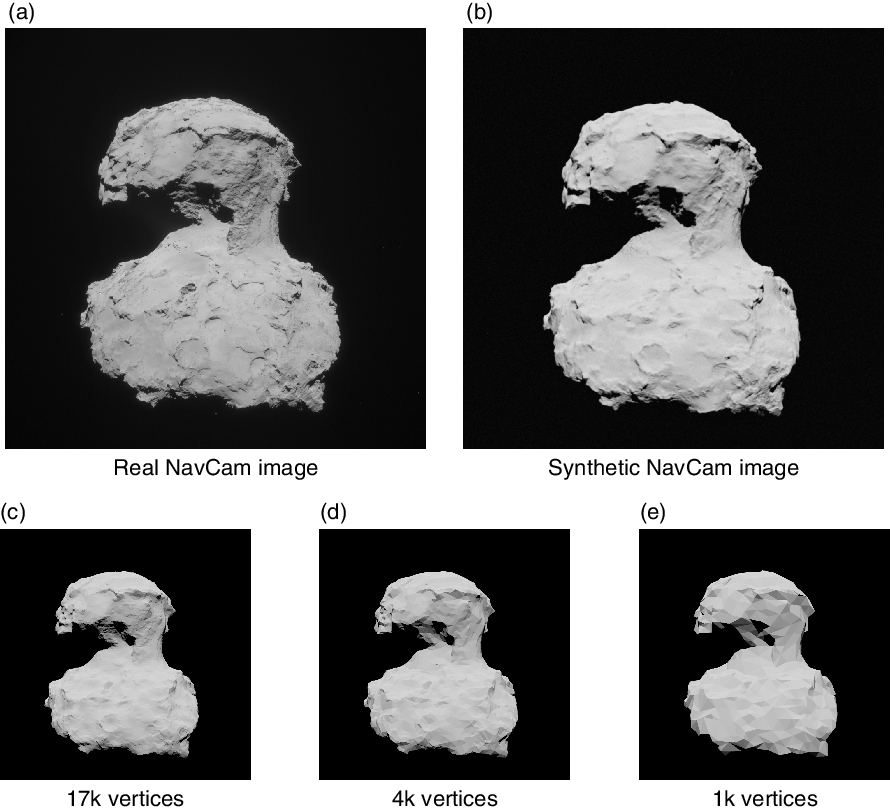
Figure 3. Five different image types were used in the study. Top left (a) is an actual preprocessed Rosetta NavCam image, top right (b) is an image rendered using a fitted Hapke reflectance model and a shape model with 1.9M vertices. Bottom row is rendered using a fitted lunar-Lambert reflectance model and shape models with varying vertex count: 17,000 (c), 4,000 (d) and 1,000 (e).
2.3 Matching and pose estimation
Matching of the features extracted from the current scene with a set of known features is done by calculating the difference of descriptors in a brute force manner and returning the closest two matches for each scene feature. Matching could also be done using FLANN(Reference Muja and Lowe44), which is a library for performing fast approximate nearest neighbor searches in high-dimensional spaces. However, we decided to use the brute force approach for simplicity. Following Lowe(Reference Lowe13), we reject most spurious matches by comparing the descriptor distance of the best match with the distance of the second best match. If the distance ratio between best and second best match is less than a certain limit, the best match is included in the set of matched features. Lowe uses a ratio limit of 0.8 but after testing different values, we decided to use 0.85 instead because it resulted in a higher number of correct matches for all the feature extraction algorithms tested.
Matched feature points define various 3D to 2D mappings, which are used to solve the relative translation and rotation between the known reference features and the current scene images using RANSAC(Reference Fischler and Bolles45), which rejects geometrically inconsistent matches. The position of the spacecraft and possibly asteroid rotation state can be updated based on the results. RANSAC uses an inner algorithm to solve the perspective-3-point (P3P) problem that gives the camera pose based on a minimal set of three known feature points. We considered various P3P solving algorithms available in OpenCV and settled on AP3P(Reference Ke and Roumeliotis46) during initial testing.
By feeding the geometrically consistent matches from RANSAC to a navigation filter(Reference Ansar and Cheng24,Reference Bayard and Brugarolas47) , the accuracy could be substantially improved. The asteroid rotation axis and rotation phase shift at epoch could be included in the filter state. These are left for future work.
All the algorithms, Monte Carlo simulation, error calculations, and Rosetta NavCam image loading were done using Python and OpenCV. The source code can be found on GitHub(Reference Knuuttila48).
3.0 RESULTS
We used Monte Carlo simulations to measure the performance of different feature extraction algorithms. For each generated sample we measured: (i) spacecraft–asteroid distance error; (ii) lateral displacement error, and; (iii) orientation error. It is practical to give the first two errors as relative to the actual distance, as this way we can remove the geometric dependency on distance for these errors. The algorithm will exit early if there are less than 12 geometrically consistent feature matches, resulting in a pose estimation failure. For each feature extraction algorithm, we generate 10,000 Monte Carlo samples, after which we calculate algorithm failure rates and percentiles of the three different error measures. Each sampling consists of the following steps:
1. Pick a random set of parameter values that defines the system state.
2. Generate noisy measurements including a NavCam image.
3. Based on measurements from the previous step, run the SPL algorithm that then gives an estimate for the relative spacecraft–asteroid pose.
4. Compare estimated pose with the real pose from step 1, calculate and log the errors.
The relevant system state can be defined by the spacecraft orientation, the asteroid rotation axis, the right ascension of asteroid zero longitude at epoch, time since epoch and the asteroid–spacecraft relative position. The relative position is sampled using spherical coordinates with uniform distribution and distance between 25 and 400km. The spacecraft orientation is sampled so that the asteroid center of volume is always contained in the FoV. The asteroid rotation axis parameters are not sampled but set to the values corresponding to the comet 67P/Churyumov–Gerasimenko. Time, which is sampled to be between 01 January 2015 and 01 January 2016, affects asteroid orientation and also the Sun–asteroid position. If the phase angle is larger than 140°, the system state is sampled again. The phase angle is the angle between the lines connecting the asteroid to the spacecraft and the asteroid to the Sun, i.e. a phase angle of 0° would mean that the whole asteroid is in the sunlight and an angle of 180° means that no sunlit areas of the asteroid can be seen.
Based on the sampled system state, the following measurements are generated for the pose estimation algorithm to use:
• Asteroid rotation axis, tilted randomly between 0° and 10°
• Asteroid zero longitude right ascension at epoch, Gaussian noise,
$\sigma = 5^{\circ}$
• Time instant determining asteroid orientation and Sun–asteroid position, noiseless measurement is used as the effect of any reasonable noise would be negligible compared to other sources of noise
• Spacecraft orientation, each Euler angle with Gaussian noise,
$\sigma = 1^{\circ}$
• A synthetic NavCam image rendered using a detailed shape model with 1.9M vertices(Reference Malmer49), a Hapke reflectance model(Reference Hapke41) and self-shadowing (see Fig. 3). Foreground pixel noise (from a normal distribution) and a starry background (from a Pareto distribution) are generated to closely match real Rosetta NavCam images.


The asteroid and spacecraft orientation noises are selected to be as high as possible – while still seeming reasonable to the authors – to better measure the robustness of the different feature extraction algorithms. For comparison, the orientation error of a typical star tracker is less than 20 arcsec (1-sigma)(Reference Fialho and Mortari50) and the uncertainty of the asteroid rotation axis longitude after extensive lightcurve observations approach 7° (1-sigma)(Reference Bowell, Oszkiewicz, Wasserman, Muinonen, Penttilä and Trilling51). On-board asteroid rotation modeling is expected to be much more accurate than this.
The reference image rendered on-board by the pose estimation algorithm is based on a less detailed shape model and the lunar–Lambert reflectance model. To investigate the effect of the vertex count on the algorithm performance, we tested each feature extraction algorithm with on-board shape models having 17,000, 4,000 and 1,000 vertices (see Fig. 3). The results are summarised in Table 2 and Fig. 4.
The failure rates in Table 2 might seem high, but the situation is not so severe, because most of the failures are due to a very difficult spacecraft position where the phase angle is high, the initial orientation error is high, the asteroid is very far, or so near that only a part is visible. If an algorithm fails to give a pose estimate for a certain image, this failure does not contribute towards the error measures. For example, ORB has the highest failure rate of 28.5% when using the 4,000 vertex shape model but then has lower errors for distance and orientation than AKAZE, which has the lowest failure rate of 16.6%. What likely occurs is that ORB fails on difficult samples and thus avoids barely successful, inaccurate pose solutions from worsening it’s error statistics. Because of this, the failure rate takes precedence when comparing the different algorithms. Only when it is similar between algorithms, can we compare the error percentiles fairly. Based on this, it seems that SIFT performs best when a reasonably detailed shape model is used, as both its failure rate and position related error percentiles are better than the others. However, when a less-detailed shape model is used, it appears that AKAZE is the best performer. For the crudest-shape model, AKAZE has a failure rate of 21.4% compared to the next best option, SURF with a 36.6% failure rate. For the middling-shape model with 4,000 vertices, the comparison between AKAZE and SIFT is more ambiguous than with the extremes. The AKAZE failure rate is 16.6% versus SIFT 20.0% while the error percentiles favor SIFT.
To investigate the operational space of the algorithms, we classified each Monte Carlo sample as a success or a failure. A sample was considered a success if the resulting orientation error was below 7°. We represented the failures and successes with respect to the different situational parameters we identified before, namely phase angle, initial orientation error, asteroid distance and an estimated percentage of the asteroid in the FoV (see Fig. 4). To make the plots clearer, we excluded situations that were deemed “not easy” on a situational dimension that was not part of that particular plot, e.g. if plotting against distance and initial orientation error, we would exclude all samples that had a high phase angle or were only partially in the FoV. The range for inclusion for distance was 50–250km, for phase angle 20–100°, for initial orientation error 0–10°, and for in-camera-view 80–100%. We also selected for further analysis only the data from using the 4,000 vertex shape model to further simplify and constrain the number of graphs.
Table 2 Monte Carlo simulation results with synthetic NavCam images

The cells with grey background correspond to the best values across methods that use the same shape model. Darker grey on Fail % column reflects the high importance of it.
a Shape model vertex count used for on-board rendering
b Average algorithm runtime on an Intel i7 7700HQ 2.8GHz laptop – useful only for rough comparison between methods
c p50 is the median and p84.1 refers to the 84.1 $^th$
percentile of the error, which corresponds to one standard deviation away from the mean for normally distributed data.
$^th$
percentile of the error, which corresponds to one standard deviation away from the mean for normally distributed data.

Figure 4. Successes (light blue) and failures (brown) of Monte Carlo samples with different feature extraction algorithms. For better sample separation when in-camera-view is exactly 100%, we add a 0–20% random component if the parameter value is 100%, so that values between 100–120% map to 100%.
Figure 4 shows that SURF and SIFT degrade less than AKAZE and ORB when the distance increases. In particular, ORB practically stops working if the distance is more than 300km while the others continue to function, provided that the situation otherwise is advantageous. ORB and AKAZE handle slightly better high phase angles than SURF and SIFT. ORB and AKAZE also seem to tolerate a high initial orientation error better. AKAZE seems most tolerant of situations when only a small part of the asteroid is in the FoV.
To understand better how the various error measures behave in different situations, we plotted the failure rate and the three different error measures as a function of distance, phase angle and initial orientation error, skipping the in-camera-view percent as relatively uninteresting (see Fig. 5). The plotted failure rate is calculated over a Gaussian sliding window with a standard deviation of one-tenth of the x-axis range. The error curves are plotted by taking the median on a sliding window with a width of one-tenth of the x-axis range. Here we also included only the “easy” situations, except for the chosen situational dimension on the x-axis. The same ranges for “easy” were used as for Fig. 4.
Table 3 Full results with real NavCam images from Rosetta

aRow and column meanings are the same as in Table 2.

Figure 5. Failure rate and errors vs different situations.
For Fig. 5, the same observations hold as was already noticed from the success-failure scatter plot. Looking at the failure rates, AKAZE seems to be most robust for most situations. It has the lowest failure rates with respect to phase angles, initial orientation errors, and distances below 250km. However for distances above 250km, SIFT seems to work best. In advantageous situations the failure rates of different algorithms are very similar, so the error medians should be comparable. In these regions, ORB seems to give the most accurate results.
We also tried the different algorithms with Rosetta NavCam images that are freely available from ESA. We used six sets of images(6): Prelanding - MTP006, Prelanding - MTP007, Comet Escort 2 - MTP017, Comet Escort 4 - MTP024, Comet Extension 1 - MTP025, and Comet Extension 1 - MTP026. Some of the images were excluded from the sets if they were e.g. almost completely black or extremely overexposed. Of a total of 3,504 images, 3,296 were used. All the images have metadata stored in a separate file, which has the asteroid–spacecraft system state as estimated by the Rosetta system. We use that state as the ground truth. Noise with the same distributions as before is added to this state before passing it to the relative pose estimation algorithms. We give the same table and figures for the results from the real NavCam images as we did for the results based on synthetic images (Table 3, Figs 6 and 7).

Figure 6. Successes (light blue) and failures (brown) in different situations based on real Rosetta NavCam images. This figure is produced the same way as 2, please refer to the image caption there.
Surprisingly, Table 3 shows that all other feature extraction methods perform quite poorly – as shown by the failure rate – compared to AKAZE, which has a comparable failure rate for the Rosetta images as it did for the synthetic images. This could be due to the dataset having more situations where AKAZE is good at. Such situations would be e.g. when the spacecraft is very close to the asteroid.
By looking at Fig. 6, we can see that AKAZE performs even better compared to the others when evaluated using real images. Especially, AKAZE shines when 67P/Churyumov– Gerasimenko is near and only partly visible or when the initial orientation error is high.
In Fig. 7 we present the failure rate and different errors when using the real images in the same way as we did for the results based on the synthetic ones. The samples covered only poorly the distances between 110–160km and farther than 230km. These areas in the plots (with 10km margins, shown in pink) should be considered highly inaccurate. Also, plots with distance or phase angle on the x-axis show discontinuities around a region where there were many samples centered on 200km distance and 90° phase angle.
As can be seen in Fig. 7, AKAZE performs best by a large margin. The phase angle does not seem to have a significant impact, at least in the range 20°–140°. The higher errors seen between 80° and 100° can be explained by the sample distribution as all distant samples were in that phase angle range. The initial orientation error seems to have a much higher impact on performance than what was expected based on the experiment with synthetic images. For AKAZE, a 10° initial orientation error seems to correspond roughly to a 7% failure rate.
Table 4 Operational zone results using AKAZE and tested with Rosetta images


Figure 7. Failure rate and errors vs different situations based on real Rosetta NavCam images. Note how AKAZE (orange lines) has the lowest failure rate and lowest errors in almost all regions.
In order to report some useful single values for the expected errors for the AKAZE-based algorithm, we define – based on Figs 6 and 7 – an operational zone for it. A sample belongs to the zone if:
• Distance to target is less than 250km
• At least 50% of the target is in the FoV
• Phase angle is less than 140°
• Initial orientation error is less than 10°
This limited our data set to 1,253 samples. The results for AKAZE with different shape model vertex counts are presented in Table 4.
By comparing the mean and standard deviation shown in Table 4 with the corresponding percentiles for a normal distribution, it is possible to estimate how close the error distribution is to it. Finally, we give some AKAZE example solutions in Figs 8 and 9 to illustrate the algorithm performance when presented with some non-ideal NavCam images. On the left, there is a Rosetta NavCam image next to a reference image rendered on-board from a shape model with 4,000 vertices at a distance of 70km and with an inaccurate initial orientation. On the right, there is the same pair of images joined by lines representing those matches that are retained (inlier matches) after RANSAC has eliminated all geometrically inconsistent ones. Red circles show all features points that were not matched successfully. Images are not normalised in any way as AKAZE does not require it.

Figure 8. AKAZE features from overexposed NavCam image matched with features from onboard rendered 4,000 vertex shape model.

Figure 9. Illustration of feature matches when the comet is only partially visible. The algorithm is close to failing as there are so few inlier matches.
4.0 DISCUSSION
In the operational zone defined based on our experiments, a conservatively sized shape model with 4,000 vertices gives an average distance error of 6.3m/km and a lateral error of 0.32m/km. The average orientation error was 1.1. The accuracy can be improved slightly by using a more detailed shape model. Also, it is worth bearing in mind that this is not the final navigation accuracy as the estimates given by our algorithm should be fed into a navigation filter, which then outputs the final pose estimate.
Interesting and immediate directions for future work would be to (i) assess how a filtering scheme affects the accuracy and robustness of the system, (ii) what changes to the algorithm are needed so that it works reliably in a double-asteroid system, (iii) try to implement the algorithm in suitable hardware and (iv) try to improve synthetic NavCam image generation by using a texture map on the shape model or generating high-frequency features into it.
To increase accuracy and operational range, an integrated visual odometry scheme could be formulated, where new opportunistic features could be added on-the-fly to a feature database and later queried based on the initial pose estimate. These features could be mixed in with the SPL features detected from the synthetic reference image.
Another supplement could be to implement an approach based on deep learning to estimate the pose of the spacecraft relative to the asteroid without any initial pose estimate. This could be used in cases where we have lost the ability to generate a good enough initial pose estimate, e.g. due to an anomaly affecting the use of the star tracker or on-board clock.
5.0 CONCLUSION
We have shown that synthetic image generation together with local photometric features can be used for medium-range absolute navigation near an asteroid. The algorithm does not have limitations regarding the target size, axial tilt, and the existence of craters. We tested four feature-detection and -description algorithms using synthetic and real Rosetta NavCam images and compared the resulting performance under different environmental conditions. Related studies have typically included SIFT, SURF, and ORB but overlooked AKAZE, which proved to be most suitable to our application by a high margin. Using the results, we defined an operational zone for our AKAZE-based algorithm and reported its performance when using shape models of three different levels of detail. The analysis provides important information when considering vision-based navigation systems for future space missions.
ACKNOWLEDGEMENTS
The authors would like to thank Dr. Juho Kannala, Professor of Computer Vision at Aalto University for guidance in the early stages of this work, and Markku Alho, a doctoral candidate of space science and technology at Aalto University for assistance with the different shape models of the comet 67P/Churyumov–Gerasimenko.


