


1. Introduction
Buoyancy-driven convection of a diffusive boundary layer induced by concentration gradients is a subject widely explored in the literature (Riaz et al. Reference Riaz, Hesse, Tchelepi and Orr2006; Slim Reference Slim2014; Emami-Meybodi et al. Reference Emami-Meybodi, Hassanzadeh, Green and Ennis-King2015). The typical set-up giving rise to unstable behaviour is one where the vertical transient concentration gradient is directed downwards. Such Darcy–Bénard-like configuration pertains to a diffusive boundary layer that grows with time and becomes gravitationally unstable under certain circumstances. The evolution of instabilities forms the fingers of a dense fluid penetrating into a lighter underlying fluid, which results in natural convection. This convective mixing significantly enhances the rate of mass transfer, rather than relying on slow mass transfer by diffusion.
Much research has been done to investigate the buoyancy-driven convection in fluid-saturated porous media since the pioneering work of Horton & Rogers (Reference Horton and Rogers1945) and Lapwood (Reference Lapwood1948) for thermal convection. Most of the studies investigating thermoconvective instability of a motionless base state are related to a horizontal layer with impermeable and isothermal walls kept at different temperatures, which is known as the Darcy–Bénard problem (Nield & Bejan Reference Nield and Bejan2017). The Darcy–Bénard problem has been extended to an inclined porous layer in the pioneering studies by Bories & Combarnous (Reference Bories and Combarnous1973) and Weber (Reference Weber1974). The main consequence of the layer inclination is that the base state would have a stationary and parallel buoyant flow with a zero mass flow rate. Recent studies have shed light on the instability of the Darcy–Bénard problem in inclined systems (Rees & Bassom Reference Rees and Bassom2000; Rees, Storesletten & Postelnicu Reference Rees, Storesletten and Postelnicu2006; Barletta & Storesletten Reference Barletta and Storesletten2011; Sphaier, Barletta & Celli Reference Sphaier, Barletta and Celli2015).
The solutal convective instability has received significant attention over the past two decades due to its application to the storage of carbon dioxide (CO2) in deep saline aquifers (Hassanzadeh, Pooladi-Darvish & Keith Reference Hassanzadeh, Pooladi-Darvish and Keith2005; Bolster Reference Bolster2014; Emami-Meybodi et al. Reference Emami-Meybodi, Hassanzadeh, Green and Ennis-King2015). Most studies examined the process of solute convection in a Darcy–Bénard-like configuration for a horizontal layer with a Dirichlet-type boundary condition for the solute concentration while imposing zero flux at the top and assuming single-phase flow. This simplification ignores the capillary transition zone that may exist between two partially miscible fluids, i.e. the non-wetting CO2 phase and the wetting water phase. The capillary transition zone allows the vertical flow of the diffusive boundary layer, potentially decreasing the onset time of instability. The effects of the capillary transition zone on solutal convective instabilities have been studied by using either a permeable upper boundary condition in a single-phase system (Slim & Ramakrishnan Reference Slim and Ramakrishnan2010; Elenius, Nordbotten & Kalisch Reference Elenius, Nordbotten and Kalisch2012; Kim Reference Kim2015) or a transition zone in a two-phase system (Emami-Meybodi & Hassanzadeh Reference Emami-Meybodi and Hassanzadeh2013; Emami-Meybodi Reference Emami-Meybodi2017; Zhang & Emami-Meybodi Reference Zhang and Emami-Meybodi2018). In all these studies, a perfectly horizontal porous layer is considered to examine the solutal convection instability of a motionless base state.
This study aims to go beyond the analysis of two-phase buoyancy-driven flow in a horizontal porous layer by devising an inclined set-up where a capillary transition zone is formed between a non-wetting and a denser wetting phase. In particular, the critical role of the layer inclination on the onset of instability is examined for buoyancy-dominant, in-transition and capillary-dominant systems. The diffusion of solute from the non-wetting phase into the underlying wetting region may increase the density of the wetting phase and create a gravitationally unstable diffusive boundary layer beneath the capillary transition zone. While the dense diffusive boundary layer can potentially create solutal convective instabilities, the gravity-driven flow that arises from the variation of wetting-phase density across the inclined porous layer may delay the onset of natural convection. Hence, the base state of the problem under consideration deals with transient concentration and through flow profiles. Details about the system under consideration are described in § 2.1 (see figure 1).

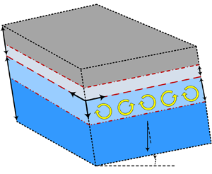
Figure 1. Geometry and coordinates of the inclined three-dimensional two-phase, two-component, partially miscible system with a capillary transition zone h formed between the wetting and non-wetting phases. The capillary transition zone and the underlying wetting-phase region (–h ≤ z ≤ H) are considered to conduct linear stability analysis. At time zero, the wetting phase in the capillary transition zone is saturated with the diffusive species  ${c_d} = c_d^\ast $ (grey shaded area), while the wetting-phase domain is free of solute concentration cd = 0 (blue shaded area). Solute gradually diffuses into the wetting-phase region and creates a diffusive boundary layer with a penetration depth of δ(t). As the diffusive boundary layer grows with time, it becomes denser and may result in natural convection.
The analysis to be carried out is an extension of the work by Emami-Meybodi & Hassanzadeh (Reference Emami-Meybodi and Hassanzadeh2013) and Zhang & Emami-Meybodi (Reference Zhang and Emami-Meybodi2018) with reference to the special case of a two-dimensional horizontal layer. This analysis considers a three-dimensional, two-phase (e.g. supercritical CO2 as non-wetting phase and brine as the wetting phase), two-component (e.g. CO2 and H2O) system in an inclined saturated porous medium, which is further described in § 2. In that section, the governing equations and the boundary conditions are also discussed. The dimensional analysis presented therein demonstrates that the two-phase, partially miscible, inclined system under consideration can be explored with five parameters, namely: viscosity ratio, gravity number, material parameter, Bond number and inclination angle. Section 3 provides the base state solutions for the saturation, velocity and concentration fields, around which the model is linearized. This includes a new time–space flow equation for the gravity-driven flow of the wetting phase through the porous medium. Section 3 also presents the linear stability formulations and discusses the quasi-steady-state approximation and the computational techniques that are used to solve a differential eigenvalue problem composed of a system of three complex-valued equations. Section 4 discusses the results of the linear stability analysis and shows the stabilizing effect of the inclination angle for different systems with different Bond numbers. The results obtained herein reveal the critical role of inclination angle on the stability of a diffusive boundary layer in the presence of a capillary transition zone and cast new light on future investigations concerning the stability of convective flow systems. Finally, § 5 summarizes the main conclusions of the present study.
2. Mathematical model
2.1. Conceptual model
During the active phase of CO2 injection into a deep saline aquifer, CO2 is forced radially outwards, assuming a vertical completion of injection wells. Away from the wells, CO2 rises due to buoyancy and spreads out to form a thin plume beneath the overlying caprock. The plume then continues to migrate in horizontal directions (x- and y-directions). To make theoretical progress, most previous theoretical studies (Ennis-King & Paterson Reference Ennis-King and Paterson2005; Riaz et al. Reference Riaz, Hesse, Tchelepi and Orr2006; Hassanzadeh, Pooladi-Darvish & Keith Reference Hassanzadeh, Pooladi-Darvish and Keith2007; Ghesmat, Hassanzadeh & Abedi Reference Ghesmat, Hassanzadeh and Abedi2011; Slim Reference Slim2014; Daniel, Riaz & Tchelepi Reference Daniel, Riaz and Tchelepi2015; Emami-Meybodi et al. Reference Emami-Meybodi, Hassanzadeh, Green and Ennis-King2015) make two simplifications. The first simplification is to recognize that the time scales for diffusion and free convection to become significant are typically much longer than the time for the injection phase and the establishment of a plume beneath the caprock. Even for a plume migrating updip, which could be slow for small updip angles, local CO2 saturation will still be typically stabilized much more quickly than free convection can be established. The second common simplification is to consider an infinite lateral extent for the CO2 plume because the length and width of the CO2 plume are significantly larger than the size of natural convection cells. Thus, our analysis begins with CO2 distributed in a laterally very extensive plume (i.e. the lateral extents in both x- and y-directions are infinite) of constant thickness spread beneath the caprock, assuming that the processes that created that distribution are faster than those examined in this study.
We considered an inclined three-dimensional, two-phase (i.e. wetting phase and non-wetting phase), two-component system (solute in the non-wetting phase and solvent in the wetting phase), as depicted figure 1. The inclined porous layer has an inclination angle of β ∈ [0°, 90°] to the horizontal. We assumed that the saturated porous medium is non-deformable, isotropic and homogeneous with a height of H + Hc, where Hc and H are the heights of the gas cap and wetting-phase layer, respectively. A capillary transition zone with a height of h was considered between the wetting and non-wetting phases because of gravity–capillary equilibration. The solute in the gas cap diffuses into the underlying porous layer saturated with the wetting phase. A Cartesian coordinate system was chosen, in which the x-axis is along the porous medium and the z-axis is positive downwards. The origin of the space coordinates is at the interface between Hc and H. The capillary transition zone combined with the underlying wetting-phase region (−h ≤ z ≤ H) was considered as the domain of study. In this domain, gravity is oriented downwards and deviates from the z-axis by β. The lower boundary of the domain was considered to be impermeable with zero mass flux and the upper boundary was maintained at constant pressure (p = pi) and concentration  $({c_d} = c_d^\ast )$, where $c_d^\ast $ is the maximum concentration of the diffusive species in the wetting phase. At time zero, the wetting-phase domain was free of solute concentration (cd = 0). We assumed that the Boussinesq approximation and Darcy's law are valid.
2.2. Governing equations
The governing equations to describe the two-phase system are given by the multiphase extension of Darcy's law, the convection–diffusion equation and the continuity equations (Aziz & Settari Reference Aziz and Settari1979; Chen, Huan & Ma Reference Chen, Huan and Ma2006):
 \begin{gather}{\boldsymbol{v}_l} ={-} \frac{{k{k_{rl}}}}{{{\mu _l}}}(\boldsymbol{\nabla }{p_l} - {\rho _l}g\boldsymbol{\nabla }z),\quad l = n,w,\end{gather}
 \begin{gather}\phi \frac{\partial }{{\partial t}}\sum\limits_{l = n,w} {{s_l}{\rho _l}{c_{dl}}} ={-} \boldsymbol{\nabla }\boldsymbol{\cdot }\sum\limits_{l = n,w} {({\boldsymbol{v}_l}{c_{dl}} - \phi {s_l}{D_{0l}}\boldsymbol{\nabla }{c_{dl}})} ,\end{gather}
 \begin{gather}\varphi \frac{\partial }{{\partial t}}\sum\limits_{l = n,w} {{s_l}{\rho _l}} + \boldsymbol{\nabla }\boldsymbol{\cdot }\sum\limits_{l = n,w} {{\rho _l}{\boldsymbol{v}_l}} = 0.\end{gather}
These are constrained by the following relations:
 \begin{equation}{s_n} + {s_w} = 1,\quad {p_c} = {p_n} - {p_w}.\end{equation}
In the above equations,  $\boldsymbol{v} = [u,v,w]$ is the Darcy velocity vector, u, v and w are the velocity components in the x-, y- and z-directions, respectively, p is the fluid pressure, pc is the capillary pressure, k is the absolute permeability, μ is the viscosity, ρ is the density, s is the saturation, kr is the relative permeability, g is the gravitational acceleration, t is the time, ϕ is the porosity, cd is the concentration of the diffusive species, D 0 is the effective diffusion coefficient, and subscripts w and n denote the wetting phase and non-wetting phase, respectively.
We assumed that the wetting-phase density, ρw, is a linear function of the concentration of the diffusive species,  ${c_{dw}}$:
 \begin{equation}{\rho _w} = {\rho _{w0}}(1 + {b_c}{c_{dw}}),\quad {b_c} = \frac{1}{{{\rho _w}}}\frac{{\partial {\rho _w}}}{{\partial {c_{dw}}}},\end{equation}
where ρw 0 is the density of the wetting phase at cdw = 0 and bc can be obtained from an equation of state.
The capillary pressure is a function of the phase saturations and can be obtained from the Leverett J-function (Leverett Reference Leverett1941):
 \begin{equation}J({s_w}) = \frac{{{p_c}}}{{({\rho _{w0}} - {\rho _n})gh}} = \sqrt {\frac{k}{\phi }} \frac{{{p_c}}}{{\wp \cos \theta }},\end{equation}
where  $\wp $ is the surface tension between the non-wetting and wetting phase and θ is the contact angle between the fluid interfaces and the rock surface.
We used the height of capillary pressure,  $h\sim \wp \cos \theta /({\rho _{w0}} - {\rho _n})g\sqrt {{k / \phi }} $, as a measure of the capillary force and adopted the van Genuchten–Mualem model for the relative permeabilities and capillary pressure relations (Mualem Reference Mualem1976; van Genuchten Reference Van Genuchten1980):
 \begin{equation}{k_{rn}} = {(1 - S)^{1/3}}{(1 - {S^{1/m}})^{2m}},\quad {k_{rw}} = {S^{1/2}}{(1 - {(1 - {S^{1/m}})^m})^2},\quad J = {({S^{ - 1/m}} - 1)^{1/n}},\end{equation}
where  $S = ({s_w} - {s_{wr}})/(1 - {s_{wr}})$, swr is the residual saturation of the wetting phase, $m = 1 - 1/n$ and n > 1 is the material parameter.
2.3. Dimensionless formulation
For the stability analysis, the domain bottom boundary, and hence the domain thickness H, has no effect on the initial development of instability because, at early times, when the diffusive boundary layer is very thin, the domain behaves as a semi-infinite medium in the z-direction. This allows us to use the ratio of diffusion to buoyancy velocity as an internal length scale (Riaz et al. Reference Riaz, Hesse, Tchelepi and Orr2006; Slim & Ramakrishnan Reference Slim and Ramakrishnan2010; Andres & Cardoso Reference Andres and Cardoso2011; Emami-Meybodi Reference Emami-Meybodi2017) for the stability problem under consideration. Hence, we chose Lc = D 0φ/ub as the length scale, where  $\varphi = \phi (1 - {s_{wr}})$ and ${u_b} = kg{b_c}{\rho _{w0}}c_d^\ast{/}{\mu _w}$ is the buoyancy velocity. The length scale Lc is a measure of the thickness of the diffusive boundary layer at the time of instability, i.e. when the inhibiting effects of diffusion balance the driving effect of buoyancy on the development of fluid motion, making the solutal Rayleigh number of order unity. Thus, one can expect the onset of instability to be independent of H when $H/{L_c} \gg 1$.
We normalized the governing equations by choosing D 0φ/ub as the length scale and  ${D_0}/L_c^2$ as the time scale. Accordingly, the dimensionless parameters are
 \begin{equation}{t_D} = \frac{{{D_0}}}{{L_c^2}}t,\quad {x_D} = \frac{x}{{{L_c}}},\quad {y_D} = \frac{y}{{{L_c}}},\quad {z_D} = \frac{z}{{{L_c}}},\quad C = \frac{c}{{c_d^\ast }},\quad U = \frac{u}{{{u_b}}},\quad V = \frac{v}{{{u_b}}},\quad W = \frac{w}{{{u_b}}}.\end{equation}
As mentioned earlier, we considered a semi-infinite domain in the z-direction. The perturbations responsible for the diffusive boundary layer's instability are experimentally observed to originate within the layer near the solute–wetting phase interface at zD = 0 (Spangenberg & Rowland Reference Spangenberg and Rowland1961; Elder Reference Elder1968; Blair & Quinn Reference Blair and Quinn1969; Wooding Reference Wooding1969; Green & Foster Reference Green and Foster1975). Thus, many studies approximate the vertical domain as semi-infinite and transform the vertical z-coordinate to the time-dependent variable  $\xi (z,t) = z/\sqrt {Dt} $ to build initial perturbations that reflect experimental conditions (Ben, Demekhin & Chang Reference Ben, Demekhin and Chang2002; Kim, Chung & Choi Reference Kim, Chung and Choi2004; Riaz et al. Reference Riaz, Hesse, Tchelepi and Orr2006; Kim & Choi Reference Kim and Choi2011; Meulenbroek, Farajzadeh & Bruining Reference Meulenbroek, Farajzadeh and Bruining2013). This transformation allows the flow fields to be expressed in terms of expansion functions localized within the diffusive boundary layer. Therefore, we chose a self-similar coordinate by applying the transformation $\xi = {z_D}/\sqrt {{t_D}} $ to localize the diffusion operator around the diffusive front and achieve considerable improvement in accuracy at early times. For the original layer geometry in a finite domain with a thickness of H (see figure 1), the parameter range over which the results are valid is given by $\delta ({t_D}) \sim \sqrt {{t_D}} \ll 1$, where δ is the penetration depth of the diffusive boundary layer within the wetting-phase region.
Using (2.6) and the  $\xi $ transformation, the dimensionless form of the governing equations for flow, wetting-phase saturation and concentration can be expressed as
 \begin{gather}
\dfrac{{{\partial ^2}W}}{{\partial x_D^2}} +
\dfrac{{{\partial ^2}W}}{{\partial y_D^2}} +
\dfrac{1}{{{t_D}}}\dfrac{{{\partial ^2}W}}{{\partial {\xi
^2}}} - {k_{rw}}\left( {\cos \beta \left(
{\dfrac{{{\partial^2}C}}{{\partial x_D^2}} +
\dfrac{{{\partial^2}C}}{{\partial y_D^2}}} \right) + \sin
\beta \dfrac{{{\partial^2}C}}{{\partial {x_D}\partial
{z_D}}}} \right)\notag\\ \quad - {{k^{\prime}}_{rw}}\left(
{\cos \beta \left( {\dfrac{{\partial S}}{{\partial
{x_D}}}\dfrac{{\partial C}}{{\partial {x_D}}} +
\dfrac{{\partial S}}{{\partial {y_D}}}\dfrac{{\partial
C}}{{\partial {y_D}}}} \right) + \sin \beta
\dfrac{{\partial S}}{{\partial {x_D}}}\dfrac{{\partial
C}}{{\partial {z_D}}}} \right)\notag\\ \quad -
\dfrac{{{{k^{\prime}}_{rw}}}}{{{k_{rw}}}}\left(
{\dfrac{{\partial W}}{{\partial {x_D}}}\dfrac{{\partial
S}}{{\partial {x_D}}} + \dfrac{{\partial W}}{{\partial
{y_D}}}\dfrac{{\partial S}}{{\partial {y_D}}} + W\left(
{\dfrac{{{\partial^2}S}}{{\partial x_D^2}} +
\dfrac{{{\partial^2}S}}{{\partial y_D^2}}} \right) +
\dfrac{1}{{{t_D}}}\dfrac{{\partial S}}{{\partial \xi
}}\dfrac{{\partial W}}{{\partial \xi }} - \dfrac{1}{{\sqrt
{{t_D}} }}\left( {U\dfrac{{{\partial^2}S}}{{\partial
{x_D}\partial \xi }} + V\dfrac{{{\partial^2}S}}{{\partial
{y_D}\partial \xi }}} \right)} \right)\notag\\ \quad - {\left(
{\dfrac{{{{k^{\prime}}_{rw}}}}{{{k_{rw}}}}} \right)^\prime
}\left( {W\left[ {{{\left( {\dfrac{{\partial S}}{{\partial
{y_D}}}} \right)}^2} + {{\left( {\dfrac{{\partial
S}}{{\partial {x_D}}}} \right)}^2}} \right] -
\dfrac{1}{{\sqrt {{t_D}} }}\dfrac{{\partial S}}{{\partial
\xi }}\left( {U\dfrac{{\partial S}}{{\partial {x_D}}} +
V\dfrac{{\partial S}}{{\partial {y_D}}}} \right)} \right) =
0, \end{gather}
\begin{gather}
\dfrac{{{\partial ^2}W}}{{\partial x_D^2}} +
\dfrac{{{\partial ^2}W}}{{\partial y_D^2}} +
\dfrac{1}{{{t_D}}}\dfrac{{{\partial ^2}W}}{{\partial {\xi
^2}}} - {k_{rw}}\left( {\cos \beta \left(
{\dfrac{{{\partial^2}C}}{{\partial x_D^2}} +
\dfrac{{{\partial^2}C}}{{\partial y_D^2}}} \right) + \sin
\beta \dfrac{{{\partial^2}C}}{{\partial {x_D}\partial
{z_D}}}} \right)\notag\\ \quad - {{k^{\prime}}_{rw}}\left(
{\cos \beta \left( {\dfrac{{\partial S}}{{\partial
{x_D}}}\dfrac{{\partial C}}{{\partial {x_D}}} +
\dfrac{{\partial S}}{{\partial {y_D}}}\dfrac{{\partial
C}}{{\partial {y_D}}}} \right) + \sin \beta
\dfrac{{\partial S}}{{\partial {x_D}}}\dfrac{{\partial
C}}{{\partial {z_D}}}} \right)\notag\\ \quad -
\dfrac{{{{k^{\prime}}_{rw}}}}{{{k_{rw}}}}\left(
{\dfrac{{\partial W}}{{\partial {x_D}}}\dfrac{{\partial
S}}{{\partial {x_D}}} + \dfrac{{\partial W}}{{\partial
{y_D}}}\dfrac{{\partial S}}{{\partial {y_D}}} + W\left(
{\dfrac{{{\partial^2}S}}{{\partial x_D^2}} +
\dfrac{{{\partial^2}S}}{{\partial y_D^2}}} \right) +
\dfrac{1}{{{t_D}}}\dfrac{{\partial S}}{{\partial \xi
}}\dfrac{{\partial W}}{{\partial \xi }} - \dfrac{1}{{\sqrt
{{t_D}} }}\left( {U\dfrac{{{\partial^2}S}}{{\partial
{x_D}\partial \xi }} + V\dfrac{{{\partial^2}S}}{{\partial
{y_D}\partial \xi }}} \right)} \right)\notag\\ \quad - {\left(
{\dfrac{{{{k^{\prime}}_{rw}}}}{{{k_{rw}}}}} \right)^\prime
}\left( {W\left[ {{{\left( {\dfrac{{\partial S}}{{\partial
{y_D}}}} \right)}^2} + {{\left( {\dfrac{{\partial
S}}{{\partial {x_D}}}} \right)}^2}} \right] -
\dfrac{1}{{\sqrt {{t_D}} }}\dfrac{{\partial S}}{{\partial
\xi }}\left( {U\dfrac{{\partial S}}{{\partial {x_D}}} +
V\dfrac{{\partial S}}{{\partial {y_D}}}} \right)} \right) =
0, \end{gather} \begin{gather}
\dfrac{{\partial S}}{{\partial {t_D}}} - \dfrac{\xi
}{{2{t_D}}}\dfrac{{\partial S}}{{\partial \xi }} -
\dfrac{{{f^\prime }}}{f}\left( {U\dfrac{{\partial
S}}{{\partial {x_D}}} + V\dfrac{{\partial S}}{{\partial
{y_D}}} + \dfrac{W}{{\sqrt {{t_D}} }}\dfrac{{\partial
S}}{{\partial \xi }}} \right)\notag\\ \quad + \,
\dfrac{G}{{Bo\,f}}\left( {{{({k_{rn}}J^{\prime})}^\prime
}\left( {{{\left( {\dfrac{{\partial S}}{{\partial {x_D}}}}
\right)}^2} + {{\left( {\dfrac{{\partial S}}{{\partial
{y_D}}}} \right)}^2} + \dfrac{1}{{{t_D}}}{{\left(
{\dfrac{{\partial S}}{{\partial \xi }}} \right)}^2}}
\right) + {k_{rn}}J^{\prime}\left(
{\dfrac{{{\partial^2}S}}{{\partial x_D^2}} +
\dfrac{{{\partial^2}S}}{{\partial y_D^2}} +
\dfrac{1}{{{t_D}}}\dfrac{{{\partial^2}S}}{{\partial
{\xi^2}}}} \right)} \right)\notag\\ \quad +\, \dfrac{{\cos \beta
}}{{f\sqrt {{t_D}} }}\left( {{k_{rn}}\dfrac{{\partial
C}}{{\partial \xi }} + {{k^{\prime}}_{rn}}(C +
G)\dfrac{{\partial S}}{{\partial \xi }}} \right) -
\dfrac{{\sin \beta }}{f}\left( {{k_{rn}}\dfrac{{\partial
C}}{{\partial {x_D}}} + (C +
G){{k^{\prime}}_{rn}}\dfrac{{\partial S}}{{\partial
{x_D}}}} \right) = 0 \end{gather}
\begin{gather}
\dfrac{{\partial S}}{{\partial {t_D}}} - \dfrac{\xi
}{{2{t_D}}}\dfrac{{\partial S}}{{\partial \xi }} -
\dfrac{{{f^\prime }}}{f}\left( {U\dfrac{{\partial
S}}{{\partial {x_D}}} + V\dfrac{{\partial S}}{{\partial
{y_D}}} + \dfrac{W}{{\sqrt {{t_D}} }}\dfrac{{\partial
S}}{{\partial \xi }}} \right)\notag\\ \quad + \,
\dfrac{G}{{Bo\,f}}\left( {{{({k_{rn}}J^{\prime})}^\prime
}\left( {{{\left( {\dfrac{{\partial S}}{{\partial {x_D}}}}
\right)}^2} + {{\left( {\dfrac{{\partial S}}{{\partial
{y_D}}}} \right)}^2} + \dfrac{1}{{{t_D}}}{{\left(
{\dfrac{{\partial S}}{{\partial \xi }}} \right)}^2}}
\right) + {k_{rn}}J^{\prime}\left(
{\dfrac{{{\partial^2}S}}{{\partial x_D^2}} +
\dfrac{{{\partial^2}S}}{{\partial y_D^2}} +
\dfrac{1}{{{t_D}}}\dfrac{{{\partial^2}S}}{{\partial
{\xi^2}}}} \right)} \right)\notag\\ \quad +\, \dfrac{{\cos \beta
}}{{f\sqrt {{t_D}} }}\left( {{k_{rn}}\dfrac{{\partial
C}}{{\partial \xi }} + {{k^{\prime}}_{rn}}(C +
G)\dfrac{{\partial S}}{{\partial \xi }}} \right) -
\dfrac{{\sin \beta }}{f}\left( {{k_{rn}}\dfrac{{\partial
C}}{{\partial {x_D}}} + (C +
G){{k^{\prime}}_{rn}}\dfrac{{\partial S}}{{\partial
{x_D}}}} \right) = 0 \end{gather}and
 \begin{align}& S\dfrac{{\partial C}}{{\partial {t_D}}} - S\dfrac{\xi
}{{2{t_D}}}\dfrac{{\partial C}}{{\partial \xi }} -
\dfrac{{\partial S}}{{\partial {x_D}}}\dfrac{{\partial
C}}{{\partial {x_D}}} - \dfrac{{\partial S}}{{\partial
{y_D}}}\dfrac{{\partial C}}{{\partial {y_D}}} -
\dfrac{1}{{{t_D}}}\dfrac{{\partial S}}{{\partial \xi
}}\dfrac{{\partial C}}{{\partial \xi }}\notag\\ &\quad + \,
U\dfrac{{\partial C}}{{\partial {x_D}}} + V\dfrac{{\partial
C}}{{\partial {y_D}}} + \dfrac{W}{{\sqrt {{t_D}}
}}\dfrac{{\partial C}}{{\partial \xi }} - S\left(
{\dfrac{{{\partial^2}C}}{{\partial x_D^2}} +
\dfrac{{{\partial^2}C}}{{\partial y_D^2}} +
\dfrac{1}{{{t_D}}}\dfrac{{{\partial^2}C}}{{\partial
{\xi^2}}}} \right) = 0, \end{align}
\begin{align}& S\dfrac{{\partial C}}{{\partial {t_D}}} - S\dfrac{\xi
}{{2{t_D}}}\dfrac{{\partial C}}{{\partial \xi }} -
\dfrac{{\partial S}}{{\partial {x_D}}}\dfrac{{\partial
C}}{{\partial {x_D}}} - \dfrac{{\partial S}}{{\partial
{y_D}}}\dfrac{{\partial C}}{{\partial {y_D}}} -
\dfrac{1}{{{t_D}}}\dfrac{{\partial S}}{{\partial \xi
}}\dfrac{{\partial C}}{{\partial \xi }}\notag\\ &\quad + \,
U\dfrac{{\partial C}}{{\partial {x_D}}} + V\dfrac{{\partial
C}}{{\partial {y_D}}} + \dfrac{W}{{\sqrt {{t_D}}
}}\dfrac{{\partial C}}{{\partial \xi }} - S\left(
{\dfrac{{{\partial^2}C}}{{\partial x_D^2}} +
\dfrac{{{\partial^2}C}}{{\partial y_D^2}} +
\dfrac{1}{{{t_D}}}\dfrac{{{\partial^2}C}}{{\partial
{\xi^2}}}} \right) = 0, \end{align}
where  $f = M + {k_{rn}}/{k_{rw}}$, M = μ n/μ w is the viscosity ratio and primes denote derivatives with respect to the saturation of the wetting phase.
As mentioned earlier, we considered the capillary transition zone combined with the underlying wetting-phase region as the domain of study. Accordingly, (2.7) is subject to the following conditions:
 \begin{gather}W({z_D} ={-} 1/Bo) = W({z_D} = 0) = W({z_D} \to \infty ) = 0,\end{gather}
 \begin{gather}V({z_D} ={-} 1/Bo) = V({z_D} = 0) = V({z_D} \to \infty ) = 0,\end{gather}
 \begin{gather}U({z_D} ={-} 1/Bo) = U({z_D} \to \infty ) = 0,\end{gather}
 \begin{gather}S({z_D} ={-} 1/Bo) = 0,\quad S({z_D} = 0) = S({z_D} \to \infty ) = 1,\end{gather}
 \begin{gather}C({z_D} ={-} 1/Bo) = C({z_D} = 0) = 1,\quad C({z_D} \to \infty ) = 0.\end{gather}
 According to (2.8), besides U at  ${z_D} = 0$, other variables are subject to three known boundary conditions since the base state solutions for the capillary transition zone $( - 1/{B_o} \le {z_D} \le 0)$ and the wetting-phase region $(0 \le {z_D} \to \infty )$ were obtained separately using the same boundary conditions at ${z_D} = 0$. Furthermore, U at zD = 0 was obtained from the base state solution by applying the condition U = 0 when C = 0.
As noted from (2.7), the system under consideration can be explored with reference to the Bond number, Bo = Lc/h, gravity number, G = k(ρ w0 − ρn)g/u bμ w, viscosity ratio, M = μ n/μ w, material parameter, n, and inclination angle, β.
Based on the schematic of the CO2–water system shown in figure 1, the displacement takes place in the z-direction, and the denser fluid with the higher viscosity (water as the wetting phase) is located under the lighter fluid with the lower viscosity (CO2 as the non-wetting phase). Such a two-phase system remains stable in the absence of solute diffusion into the wetting phase because (μ w/k rw − μ n/k rn)(U 0 − Uc) always remains a negative value (Marle Reference Marle1981), where Uc = k(ρ w0 − ρn)g/(μ w/k rw − μ n/k rn) and U 0 is the base state advective velocity, which is zero for the problem under consideration. Therefore, G and M do not affect the instability of the two-phase system because the denser water with the higher viscosity is located under the lighter CO2 with the lower viscosity (Emami-Meybodi Reference Emami-Meybodi2017). In this study, we used fixed values of G = 10 and M = 0.1, representing the CO2–water system.
The Bond number is a measure of the relative strength of gravitational forces to capillary forces where the limit Bo → ∞ recovers the single-phase system in which h → 0. The two-phase system can be divided into three categories based on the Bo value: buoyancy-dominant systems for Bo > 102; in-transition systems for 10−3 < Bo < 102; and capillary-dominant systems for Bo < 10−3 (Emami-Meybodi & Hassanzadeh Reference Emami-Meybodi and Hassanzadeh2013; Zhang & Emami-Meybodi Reference Zhang and Emami-Meybodi2018). We used a wide range of 10−3 ≤ Bo ≤ 103 in this study to investigate the onset of instability for all three systems.
The material parameter n > 1 is a measure of the pore-size distribution, which depends on the degree of sorting of the grains in a porous medium. For the in-transition systems with 10−3 < Bo < 102, the positive effect of the material parameter on the onset of convection has been demonstrated using linear stability analysis (LSA; Zhang & Emami-Meybodi Reference Zhang and Emami-Meybodi2018) and direct numerical simulations (Emami-Meybodi & Hassanzadeh Reference Emami-Meybodi and Hassanzadeh2015). Larger values of n for in-transition systems reflect higher wetting-phase saturation just above the interface between the wetting and non-wetting phases, which means higher crossflow across the interface. Nonetheless, the material parameter has no significant influence on the onset of instability for the buoyancy-dominant and the capillary-dominant systems (Emami-Meybodi & Hassanzadeh Reference Emami-Meybodi and Hassanzadeh2013; Emami-Meybodi Reference Emami-Meybodi2017; Zhang & Emami-Meybodi Reference Zhang and Emami-Meybodi2018). Considering prior investigations and the insignificant impact of the material parameter on the stability of buoyancy- and capillary-dominant systems, we used a fixed value of n = 3 (υ = 10) in this study, where υ is a constant assigned according to the value of n that ensures sw = swr at z = –h.
3. Formulation of the stability problem
3.1. Base state solutions
We used the definition of the J-function  $J ={-} (\cos \beta )Bo\,{z_D}$, (2.5c) and (2.8d,e) to obtain the base state solution for the wetting-phase saturation, S 0:
 \begin{equation}{S_0}({z_D}) = 1 + \boldsymbol{H}( - {z_D})[{(1 + {( - \upsilon (\cos \beta )Bo\,{z_D})^n})^{(1 - n)/n}} - 1], \end{equation}
where H is the Heaviside step function with H(x) = 0 for x < 0 and H(x) = 1 for x ≥ 0.
The base state solution for concentration (C 0) can be found from (2.7c) and (2.8f,g) using the Laplace transform (Farlow Reference Farlow1993)
 \begin{equation}{C_0}({z_D},{t_D}) = 1 - \boldsymbol{H}({z_D})erf \left( {\frac{{{z_D}}}{{2\sqrt {{t_D}} }}} \right). \end{equation}
According to (2.8a,b), the base state solutions for the velocity components of the wetting phase in the y- (V 0) and z-directions (W 0) are  ${W_0} = {V_0} = 0$ since the system is initially subject to zero velocities in these directions. However, the velocity component in the x-direction varies with time and along the z-direction because of the wetting-phase saturation and density change in the capillary transition zone and the wetting-phase region, respectively. Hence, we first used (2.1a) for the wetting phase and (2.3a) to obtain the following differential equation for U 0:
 \begin{equation}\frac{{\partial {U_0}}}{{\partial {z_D}}} = \frac{{{{k^{\prime}}_{rw}}}}{{{k_{rw}}}}\frac{{\partial {S_0}}}{{\partial {z_D}}}{U_0} - {k_{rw}}\sin \beta \frac{{\partial {C_0}}}{{\partial {z_D}}}. \end{equation}
Equation (3.3) can be solved by applying (2.5) to get
 \begin{equation}{U_0}({z_D},{t_D}) = \boldsymbol{H}({z_D})({d_1} - (\sin \beta ){C_0}) + \boldsymbol{H}( - {z_D}){d_2}{\left( {\psi \frac{{{{( - \psi {z_D})}^{n - 1}} - {{({{( - \psi {z_D})}^n} + 1)}^{(n - 1)/n}}}}{{{{({{( - \psi {z_D})}^n} + 1)}^{5(n - 1)/4n}}}}} \right)^2}, \end{equation}
where  $\psi = \upsilon (\cos \beta )Bo$ and d 1 and d 2 are constants that can be obtained by applying (2.8c,g) and ${U_0} = 0$ at ${C_0} = 0$ to (3.4):
 \begin{equation}{d_1} = 0,\quad {d_2} ={-} \frac{{\sin \beta }}{{{\psi ^2}}}.
\end{equation}
\begin{equation}{d_1} = 0,\quad {d_2} ={-} \frac{{\sin \beta }}{{{\psi ^2}}}.
\end{equation}Combining (3.4) and (3.5) gives
 \begin{align}{U_0}({z_D},{t_D}) ={-} \sin \beta \left( {\boldsymbol{H}({z_D})\left( {erfc \left( {\frac{{{z_D}}}{{2\sqrt {{t_D}} }}} \right)} \right) + \boldsymbol{H}( - {z_D}){{\left( {\frac{{{{( - \psi {z_D})}^{n - 1}} - {{({{( - \psi {z_D})}^n} + 1)}^{(n - 1)/n}}}}{{{{({{( - \psi {z_D})}^n} + 1)}^{5(n - 1)/4n}}}}} \right)}^2}} \right).\end{align}
As noted from (3.6), the base state solution U 0 = 0 is recovered in the case of a horizontal porous medium, β = 0° (Emami-Meybodi & Hassanzadeh Reference Emami-Meybodi and Hassanzadeh2013; Zhang & Emami-Meybodi Reference Zhang and Emami-Meybodi2018). Moreover, it is evident from these equations that the base state solution is left invariant by the transformation of β →  ${\rm \pi}$ − β and x → –x.
Figure 2 illustrates, for Bo = 0.01 and 0.001, how the velocity profiles vary along the z-direction for two inclined porous media having β = 15° and 45° at tD = 25, 150 and 500. The impact of inclination angle on the velocity values is evidenced in figure 2, where the magnitude of maximum velocity, |U 0,max|, increases from 0.25 to 0.7 by changing the inclination angle from 15° to 45°. A comparison between figure 2(a) and 2(b) shows that, while the U 0,max and U 0 profiles within the wetting-phase region (zD > 0) vary with β, they remain fixed with respect to Bo. However, the U 0 profile within the capillary transition zone (zD < 0) is a function of both Bo and β. A good point is asking how such velocity behaviour is likely to affect the onset of natural convection. Stability analysis of the two-phase system is a valuable tool to find an answer.

Figure 2. Base state velocity profiles along the z-direction from (3.6), for two inclined porous media having β = 15° and 45° at tD = 25, 150 and 500 with (a) Bo = 0.01 and (b) Bo = 0.001. Other parameters are fixed: n = 3 and υ = 10.
3.2. Linear stability analysis
To conduct LSA, small disturbances of velocities U 1, V 1 and W 1, saturation S 1 and concentration C 1 were introduced; therefore, U, V, W, S and C can be written as
 \begin{align}\begin{array}{l} \{ U,V,W,S,C\} ({x_D},{y_D},\xi ,{t_D})\\ \quad = \{ {U_0},{V_0},{W_0},{S_0},{C_0}\} (\xi ,{t_D}) + \varepsilon \{ {U_1},{V_1},{W_1},{S_1},{C_1}\} (\xi ,{t_D})\,{\textrm{e}^{\textrm{i}({a_x}{x_D} + {a_y}{y_D})}} + \textrm{c}\textrm{.c}., \end{array}\end{align}
where  $\textrm{i} = \sqrt { - 1} $ and ax and ay are the real-valued dimensionless components of the wavevector (i.e. wavenumbers in the x- and y-directions, respectively), with a very small amplitude ε. The subscripts 0 and 1 represent the base state and disturbance quantities, respectively.
Note that, for the stability problem under consideration, in the early stages of the diffusive boundary layer's formation, perturbations to the layer are damped. But eventually, a critical time for linear instability,  ${\tau _c}$, is reached, after which the vertical density gradient drives the fluid motion. We used the quasi-steady-state approximation (QSSA; Morton Reference Morton1957; Lick Reference Lick1965; Robinson Reference Robinson1976) to study such a linear regime and determine the critical time τc and its corresponding wavenumber αc. QSSA assumes that the growth rate of perturbations is asymptotically faster than the evolution rate of the base state solutions, i.e. the diffusive boundary layer (Riaz et al. Reference Riaz, Hesse, Tchelepi and Orr2006; Daniel, Tilton & Riaz Reference Daniel, Tilton and Riaz2013). Thus, QSSA eliminates the time dependence of the base state by solving the perturbed equations at a frozen time $\tau $. QSSA based on the frozen time $\tau $ has been widely applied to the solutal stability problem (Riaz et al. Reference Riaz, Hesse, Tchelepi and Orr2006; Selim & Rees Reference Selim and Rees2007; Chan Kim & Kyun Choi Reference Chan Kim and Kyun Choi2012; Daniel et al. Reference Daniel, Tilton and Riaz2013; Emami-Meybodi & Hassanzadeh Reference Emami-Meybodi and Hassanzadeh2013; Tilton, Daniel & Riaz Reference Tilton, Daniel and Riaz2013; Kim Reference Kim2015).
Accordingly, the concentration (3.2) and velocity (3.6) base state solutions are assumed frozen at tD = τ, and the stability of the frozen profiles is defined by
 \begin{equation}\{ {U_1},{V_1},{W_1},{S_1},{C_1}\} (\xi ,\tau ) = \{ {U^\ast },{V^\ast },{W^\ast },{S^\ast },{C^\ast }\} (\xi )\,{\textrm{e}^{\sigma \tau }},\end{equation}
where variables defined by asterisks represent the perturbation eigenfunctions and σ is the growth rate.
Introducing the perturbed solutions (3.7) and then applying QSSA (3.8) to (2.7) and retaining terms that are first-order in ε, the disturbance equations in the self-similar coordinates can be written as
 \begin{gather}\left( {\frac{{{\partial^2}}}{{\partial {\xi^2}}} - \frac{{{{k^{\prime}}_{rw}}}}{{{k_{rw}}}}\frac{{\partial {S_b}}}{{\partial \xi }}\frac{\partial }{{\partial \xi }} - {{\tilde{\alpha }}^2}} \right){W^\ast } + {k_{rw}}\left( {{{\tilde{\alpha }}^2}\cos \beta - \textrm{i}\gamma \tilde{\alpha }\sin \beta \frac{\partial }{{\partial \xi }}} \right){C^\ast } - \textrm{i}\gamma \tilde{\alpha }(\sin \beta ){k^{\prime}_{rw}}\frac{{\partial {C_0}}}{{\partial \xi }}{S^\ast } = 0,\end{gather}
 \begin{gather}\begin{array}{l} \sqrt
\tau \dfrac{{\partial {S_0}}}{{\partial \xi
}}\dfrac{{{f^\prime }}}{f}{W^\ast } - \dfrac{{\sqrt \tau
}}{f}\left( {\cos \beta \left(
{{{k^{\prime}}_{rn}}\dfrac{{\partial {S_0}}}{{\partial \xi
}} + {k_{rn}}\dfrac{\partial }{{\partial \xi }}} \right) -
\textrm{i}\gamma \tilde{\alpha }(\sin \beta ){k_{rn}}}
\right){C^\ast }\\ \quad + \left[\vphantom{\left( \begin{array}{l}
\dfrac{{{k_{rn}}J^{\prime}}}{f}\left(
{\dfrac{{{\partial^2}}}{{\partial {\xi^2}}} -
{{\tilde{\alpha }}^2}} \right) +
2\dfrac{{{{({k_{rn}}J^{\prime})}^\prime
}}}{f}\dfrac{{\partial {S_0}}}{{\partial \xi
}}\dfrac{\partial }{{\partial \xi }}\\ + {\left(
{\dfrac{{{k_{rn}}J^{\prime}}}{f}} \right)^\prime
}\dfrac{{{\partial^2}{S_0}}}{{\partial {\xi^2}}} + {\left(
{\dfrac{{{{({k_{rn}}J^{\prime})}^\prime }}}{f}}
\right)^\prime }{\left( {\dfrac{{\partial {S_0}}}{{\partial
\xi }}} \right)^2} \end{array} \right)} \right.\frac{\xi }{2}\frac{\partial }{{\partial \xi }} +
\textrm{i}\gamma \tilde{\alpha }\frac{{\sqrt \tau
}}{f}{{k^{\prime}}_{rn}}(\sin \beta )(G + {C_0}) -
\frac{G}{{Bo}}\left( \begin{array}{l}
\dfrac{{{k_{rn}}J^{\prime}}}{f}\left(
{\dfrac{{{\partial^2}}}{{\partial {\xi^2}}} -
{{\tilde{\alpha }}^2}} \right) +
2\dfrac{{{{({k_{rn}}J^{\prime})}^\prime
}}}{f}\dfrac{{\partial {S_0}}}{{\partial \xi
}}\dfrac{\partial }{{\partial \xi }}\\ + {\left(
{\dfrac{{{k_{rn}}J^{\prime}}}{f}} \right)^\prime
}\dfrac{{{\partial^2}{S_0}}}{{\partial {\xi^2}}} + {\left(
{\dfrac{{{{({k_{rn}}J^{\prime})}^\prime }}}{f}}
\right)^\prime }{\left( {\dfrac{{\partial {S_0}}}{{\partial
\xi }}} \right)^2} \end{array} \right)\\ \quad - (\cos
\beta )\sqrt \tau \left( {(G + {C_0})\left(
{\frac{{{{k^{\prime}}_{rn}}}}{f}\frac{\partial }{{\partial
\xi }} + {{\left( {\frac{{{{k^{\prime}}_{rn}}}}{f}}
\right)}^\prime }\frac{{\partial {S_0}}}{{\partial \xi }}}
\right) + {{\left( {\frac{{{k_{rn}}}}{f}} \right)}^\prime
}\frac{{\partial {C_0}}}{{\partial \xi }}} \right)\left. \vphantom{\left( \begin{array}{l}
\dfrac{{{k_{rn}}J^{\prime}}}{f}\left(
{\dfrac{{{\partial^2}}}{{\partial {\xi^2}}} -
{{\tilde{\alpha }}^2}} \right) +
2\dfrac{{{{({k_{rn}}J^{\prime})}^\prime
}}}{f}\dfrac{{\partial {S_0}}}{{\partial \xi
}}\dfrac{\partial }{{\partial \xi }}\\ + {\left(
{\dfrac{{{k_{rn}}J^{\prime}}}{f}} \right)^\prime
}\dfrac{{{\partial^2}{S_0}}}{{\partial {\xi^2}}} + {\left(
{\dfrac{{{{({k_{rn}}J^{\prime})}^\prime }}}{f}}
\right)^\prime }{\left( {\dfrac{{\partial {S_0}}}{{\partial
\xi }}} \right)^2} \end{array} \right)}
\right]{S^\ast } - \tilde{\sigma }{S^\ast } = 0
\end{array}\end{gather}
\begin{gather}\begin{array}{l} \sqrt
\tau \dfrac{{\partial {S_0}}}{{\partial \xi
}}\dfrac{{{f^\prime }}}{f}{W^\ast } - \dfrac{{\sqrt \tau
}}{f}\left( {\cos \beta \left(
{{{k^{\prime}}_{rn}}\dfrac{{\partial {S_0}}}{{\partial \xi
}} + {k_{rn}}\dfrac{\partial }{{\partial \xi }}} \right) -
\textrm{i}\gamma \tilde{\alpha }(\sin \beta ){k_{rn}}}
\right){C^\ast }\\ \quad + \left[\vphantom{\left( \begin{array}{l}
\dfrac{{{k_{rn}}J^{\prime}}}{f}\left(
{\dfrac{{{\partial^2}}}{{\partial {\xi^2}}} -
{{\tilde{\alpha }}^2}} \right) +
2\dfrac{{{{({k_{rn}}J^{\prime})}^\prime
}}}{f}\dfrac{{\partial {S_0}}}{{\partial \xi
}}\dfrac{\partial }{{\partial \xi }}\\ + {\left(
{\dfrac{{{k_{rn}}J^{\prime}}}{f}} \right)^\prime
}\dfrac{{{\partial^2}{S_0}}}{{\partial {\xi^2}}} + {\left(
{\dfrac{{{{({k_{rn}}J^{\prime})}^\prime }}}{f}}
\right)^\prime }{\left( {\dfrac{{\partial {S_0}}}{{\partial
\xi }}} \right)^2} \end{array} \right)} \right.\frac{\xi }{2}\frac{\partial }{{\partial \xi }} +
\textrm{i}\gamma \tilde{\alpha }\frac{{\sqrt \tau
}}{f}{{k^{\prime}}_{rn}}(\sin \beta )(G + {C_0}) -
\frac{G}{{Bo}}\left( \begin{array}{l}
\dfrac{{{k_{rn}}J^{\prime}}}{f}\left(
{\dfrac{{{\partial^2}}}{{\partial {\xi^2}}} -
{{\tilde{\alpha }}^2}} \right) +
2\dfrac{{{{({k_{rn}}J^{\prime})}^\prime
}}}{f}\dfrac{{\partial {S_0}}}{{\partial \xi
}}\dfrac{\partial }{{\partial \xi }}\\ + {\left(
{\dfrac{{{k_{rn}}J^{\prime}}}{f}} \right)^\prime
}\dfrac{{{\partial^2}{S_0}}}{{\partial {\xi^2}}} + {\left(
{\dfrac{{{{({k_{rn}}J^{\prime})}^\prime }}}{f}}
\right)^\prime }{\left( {\dfrac{{\partial {S_0}}}{{\partial
\xi }}} \right)^2} \end{array} \right)\\ \quad - (\cos
\beta )\sqrt \tau \left( {(G + {C_0})\left(
{\frac{{{{k^{\prime}}_{rn}}}}{f}\frac{\partial }{{\partial
\xi }} + {{\left( {\frac{{{{k^{\prime}}_{rn}}}}{f}}
\right)}^\prime }\frac{{\partial {S_0}}}{{\partial \xi }}}
\right) + {{\left( {\frac{{{k_{rn}}}}{f}} \right)}^\prime
}\frac{{\partial {C_0}}}{{\partial \xi }}} \right)\left. \vphantom{\left( \begin{array}{l}
\dfrac{{{k_{rn}}J^{\prime}}}{f}\left(
{\dfrac{{{\partial^2}}}{{\partial {\xi^2}}} -
{{\tilde{\alpha }}^2}} \right) +
2\dfrac{{{{({k_{rn}}J^{\prime})}^\prime
}}}{f}\dfrac{{\partial {S_0}}}{{\partial \xi
}}\dfrac{\partial }{{\partial \xi }}\\ + {\left(
{\dfrac{{{k_{rn}}J^{\prime}}}{f}} \right)^\prime
}\dfrac{{{\partial^2}{S_0}}}{{\partial {\xi^2}}} + {\left(
{\dfrac{{{{({k_{rn}}J^{\prime})}^\prime }}}{f}}
\right)^\prime }{\left( {\dfrac{{\partial {S_0}}}{{\partial
\xi }}} \right)^2} \end{array} \right)}
\right]{S^\ast } - \tilde{\sigma }{S^\ast } = 0
\end{array}\end{gather}
and
 \begin{align}- \frac{{\sqrt \tau
}}{{{S_0}}}\frac{{\partial {C_0}}}{{\partial \xi }}{W^\ast
} + \frac{1}{{{S_0}}}\frac{{\partial {C_0}}}{{\partial \xi
}}\frac{{\partial {S^\ast }}}{{\partial \xi }} + \left(
{\frac{{{\partial^2}}}{{\partial {\xi^2}}} + \left(
{\frac{\xi }{2} + \frac{1}{{{S_0}}}\frac{{\partial
{S_0}}}{{\partial \xi }}} \right)\frac{\partial }{{\partial
\xi }} - {{\tilde{\alpha }}^2}} \right){C^\ast } -
\tilde{\sigma }{C^\ast } = 0,\end{align}
\begin{align}- \frac{{\sqrt \tau
}}{{{S_0}}}\frac{{\partial {C_0}}}{{\partial \xi }}{W^\ast
} + \frac{1}{{{S_0}}}\frac{{\partial {C_0}}}{{\partial \xi
}}\frac{{\partial {S^\ast }}}{{\partial \xi }} + \left(
{\frac{{{\partial^2}}}{{\partial {\xi^2}}} + \left(
{\frac{\xi }{2} + \frac{1}{{{S_0}}}\frac{{\partial
{S_0}}}{{\partial \xi }}} \right)\frac{\partial }{{\partial
\xi }} - {{\tilde{\alpha }}^2}} \right){C^\ast } -
\tilde{\sigma }{C^\ast } = 0,\end{align}
where  $\tilde{\sigma } = \sigma \tau$, $\tilde{\alpha } = \alpha \sqrt \tau $ and $\alpha = \sqrt {a_x^2 + a_y^2}$ is the horizontal wavenumber. A new parameter $\gamma = {a_x}/\alpha$ is defined in (3.9) as γ ∈ [0, 1]. The special cases γ = 0 and γ = 1 lead to longitudinal and transverse rolls, respectively, while 0 < γ < 1 defines oblique rolls. Moreover, the relative permeabilities and capillary pressure in (2.7) were decomposed using the first-order Taylor expansion $\{ {k_r},J\} = \{ {k_r},J\} ({S_0}) + {S_1}{\{ {k_r},J\} ^\prime }$.
System (3.9) may be regarded as an eigenvalue problem for complex growth rate, σ = Re(σ) + i Im(σ), as a function of α, γ, β, τ and Bo, where Re and Im denote the real and imaginary parts, respectively, of a complex number. The imaginary part of σ defines the angular frequency, whereas the real part determines the unstable (if Re(σ) > 0) or stable (if Re(σ) < 0) nature of the system. Since this study focuses on the neutral stability analysis, one considers Re(σ) = 0. Accordingly, σ is purely imaginary at onset and system (3.9) may instead be regarded as an eigenvalue problem for both τ and Im(σ) as a function of α, γ, β and Bo.
3.3. Computational domain discretization
We discretized (3.9) using a finite-difference technique in which a three-point centred Lagrange polynomial approximation was used for numerical differentiation (Singh & Bhadauria Reference Singh and Bhadauria2009). A non-uniform grid system was employed to choose finer grids in the vicinity  $\xi = 0$. The non-uniform grid spacing was obtained by $\Delta {\xi _j} = {\chi ^j}/\sum\nolimits_{k = 1}^N {{\chi ^k}} $ where N = 1000 is the number of grid blocks, χ = 1.007 is the mesh increment rate and j refers to the grid spacing index, which starts from 1 for the first grid interval at the top boundary and ends with 1000 for the last grid interval at the bottom boundary. The resulting discretized system of equations (3.9) can be expressed by a system of linear equations:
 \begin{gather}{\boldsymbol{q}_1}{\boldsymbol{W}^\ast } + {\boldsymbol{q}_2}{\boldsymbol{S}^\ast } + {\boldsymbol{q}_3}{\boldsymbol{C}^\ast } = 0,\end{gather}
 \begin{gather}{\boldsymbol{q}_4}{\boldsymbol{W}^\ast } + ({\boldsymbol{q}_5} - \tilde{\sigma }\boldsymbol{\mathsf{I}}){\boldsymbol{S}^\ast } + {\boldsymbol{q}_6}{\boldsymbol{C}^\ast } = 0,\end{gather}
 \begin{gather}{\boldsymbol{q}_7}{\boldsymbol{W}^\ast } + {\boldsymbol{q}_8}{\boldsymbol{S}^\ast } + ({\boldsymbol{q}_9} - \tilde{\sigma }\boldsymbol{\mathsf{I}}){\boldsymbol{C}^\ast } = 0,\end{gather}
where W*, S* and C* are the eigenvectors for the vertical components of velocity, saturation and concentration, respectively, q 1 − q 9 are the discretization operators related to the eigenfunctions, and I is the identity matrix. System (3.10) can be simplified by substituting (3.10a) into (3.10b,3.10c) to give
 \begin{equation}\left[ {\begin{array}{*{20}{@{}cc@{}}} {{\boldsymbol{q}_5} - {\boldsymbol{q}_4}\boldsymbol{q}_1^{ - 1}{\boldsymbol{q}_2} - \tilde{\sigma }\boldsymbol{\mathsf{I}}}&{{\boldsymbol{q}_6} - {\boldsymbol{q}_4}\boldsymbol{q}_1^{ - 1}{\boldsymbol{q}_3}}\\ {{\boldsymbol{q}_8} - {\boldsymbol{q}_7}\boldsymbol{q}_1^{ - 1}{\boldsymbol{q}_2}}&{{\boldsymbol{q}_9} - {\boldsymbol{q}_7}\boldsymbol{q}_1^{ - 1}{\boldsymbol{q}_3} - \tilde{\sigma }\boldsymbol{\mathsf{I}}} \end{array}} \right]\left[ {\begin{array}{*{20}{@{}c@{}}} {{\boldsymbol{S}^\ast }}\\ {{\boldsymbol{C}^\ast }} \end{array}} \right] = \left[ \begin{array}{@{}l@{}} 0\\ 0 \end{array} \right].\end{equation}
 System (3.11) constitutes a linear algebraic eigenvalue problem, which can be numerically solved for  $\tilde{\sigma }$ using standard techniques (Lin & Segel Reference Lin and Segel1988) once α, γ, β, τ and Bo are prescribed.
3.4. Calculation of τ and α
The previous section described how to obtain the growth rate σ, or the angular frequency Im(σ), by solving (3.11) from given values of α, γ, β, τ and Bo. But an additional step must be incorporated to draw neutral stability curves. This involves calculating τ and α from a given configuration with known γ, β and Bo. We carried out this step by enforcing a condition that Re(σ) = 0, thus satisfying the neutral stability requirement. In the MATLAB code developed, this is accomplished by incorporating the secant method (Chapra & Canale Reference Chapra and Canale2010) to find the values of τ and α that satisfy Re(σ) = 0. Furthermore, the largest eigenvalues and the corresponding eigenvectors of (3.11) were obtained to determine the critical time τc and its corresponding wavenumber αc. In other words, the evolution of the maximum value of the concentration, the saturation or the velocity eigenfunction forms the basis of the growth rate at given τ and α. The dynamical system is said to be stable if Re(σ) < 0 and a critical time τc (the onset of instability) is indicated when the growth rate just becomes positive at a critical wavenumber αc.
4. Results and discussion
We performed LSA by solving (3.11) to parametrize the effect of inclination of a saturated porous layer subject to a capillary transition zone on the growth rate of perturbations and, consequently, the onset of natural convection. We conducted LSA for a wide range of 0 ≤ γ ≤ 1, 0° ≤ β ≤ 90° and 10−3 ≤ Bo ≤ 103 but at fixed values of G = 10, M = 0.1 and n = 3. In what follows, first, the neutral stability curves for the longitudinal (γ = 0), oblique (γ = 0.5) and transverse (γ = 1) rolls are discussed. Then, critical values for the onset of the instability (αc, τc) are obtained by seeking the minimum of the neutral stability function τ(α).
4.1. Neutral stability curves
The first results are focused on the neutral stability curves for the longitudinal (γ = 0), oblique (γ = 0.5) and transverse (γ = 1) rolls. Figure 3 depicts the neutral stability curves in the plane (α, τ) with β from 0° to 45° for longitudinal rolls γ = 0. We considered a buoyancy-dominant system with Bo = 103 (negligible capillary transition zone), a capillary-dominant system with Bo = 10−3 (considerable capillary transition zone) and two in-transition systems with Bo = 0.1 and 0.01. As shown in figure 4, at a given Bo, the neutral stability curve is shrunken and shifted upwards as β increases from 0° to 45°, revealing the stabilizing effect of the inclination on the onset of instability. As one can observe from comparing these curves at different Bo, when the Bond number is very small, the neutral stability curves are less sensitive to the inclination angle. Conversely, for a larger value of Bo, the neutral stability curves move upwards significantly as β increases, thus describing the stronger impact of β in stabilizing the diffusive boundary layer in the buoyancy-dominant systems than in the capillary-dominant systems. When β becomes as small as 5°, the neutral stability curves behave very similarly to the horizontal case (β = 0), particularly for the systems with significantly small Bond numbers, i.e. Bo → 0. We note that the neutral stability curves of the longitudinal rolls (γ = 0) for the horizontal cases are identical to the results presented by Emami-Meybodi (Reference Emami-Meybodi2017) and Zhang & Emami-Meybodi (Reference Zhang and Emami-Meybodi2018).

Figure 3. Neutral stability curves in the plane (α, τ) with different Bond numbers Bo = 103, 10−1, 10−2 and 10−3, and for different inclination angles, β, from 0° to 45° in increments of 5° for longitudinal rolls γ = 0.

Figure 4. Neutral stability curves in the plane (α, τ) with different Bond numbers Bo = 103, 10−1, 10−2 and 10−3, and for different inclination angles, β, from 0° to 45° in increments of 5° for oblique rolls γ = 0.5.
Figure 4 displays neutral stability curves for oblique rolls γ = 0.5 in the plane (α, τ) with different inclination angles at Bo = 103, 10−1, 10−2 and 10−3. This figure shows that the neutral stability curves shrink and move upwards as the inclination angle increases, with larger changes for the oblique rolls than for the longitudinal rolls. This phenomenon becomes significant in the buoyancy-dominant systems having high values of Bond numbers.
Figure 5 refers to transverse rolls and displays neutral stability curves in the plane (α, τ) with different inclination angles at Bo = 103, 10−1, 10−2 and 10−3. A comparison between this figure and figures 3 and 4, within the shown vertical range, reveals that the transverse rolls are the least unstable rolls, where the natural stability curves are significantly shifted upwards. This occurrence is further intensified at high values of Bo, so that, for sufficiently large Bond numbers and a sufficiently large inclination angle. If the inclination is sufficiently high (e.g. β = 30 for the buoyancy-dominant systems and β = 50 for the capillary-dominant systems), the curves for larger values of β move upwards to such an extent that they are no longer visible within the vertical range of the plots.

Figure 5. Neutral stability curves in the plane (α, τ) with different Bond numbers Bo = 103, 10−1, 10−2 and 10−3, and for different inclination angles, β, from 0° to 45° in increments of 5° for transverse rolls γ = 1.
4.2. Critical values
After examining the neutral stability curves, the next results are focused on the critical values of time and wavenumber. Figure 6 shows the critical time and its associated critical wavenumber as functions of the inclination angle at different Bo = 103, 10−1, 10−2 and 10−3, which have been obtained by minimizing time over all wavenumbers as β increases. This figure illustrates that, at a given Bo, the critical time increases with β, whereas the critical wavenumber decreases with β. It is also interesting to note that, for small inclination angles, the dependence on β is minor, which is further reduced for smaller values of Bo. Conversely, for sufficiently large inclination angles, when β > 60°, the onset of instability sharply increases with β. In fact, at very large inclination angles, and as β → 90°, there is no dependence on Bo and there are no unstable longitudinal rolls since τc → ∞ and αc → 0.

Figure 6. Critical time τc and its corresponding wavenumber αc curves versus β at different Bond numbers Bo = 103, 10−1, 10−2 and 10−3 for longitudinal rolls γ = 0.
Further investigation of LSA results shows that, for β ≤ 60°, the critical dimensionless time and corresponding wavenumber vary exponentially with β. After testing several different exponential models, we found that for both buoyancy-dominant (Bo = 103) and capillary-dominant (Bo = 10−3) systems, when β ≤ 60°, the critical values follow the Stirling model for the onset of instability and its corresponding wavenumber:
 \begin{gather}{\tau _c} = {\tau _{c0}}[1 + 0.045({e ^{0.07\beta }} - 1)],\end{gather}
 \begin{gather}{\alpha _c} = {\alpha _{c0}}[1 - 0.077({e ^{0.034\beta }} - 1)],\end{gather}
where τc 0 and αc 0 are the critical time and wavenumber for the horizontal case (β = 1). For the buoyancy-dominant horizontal systems, the critical time and wavenumber are τc 0 = 167.6 and αc 0 = 0.0696, respectively; and, for the capillary-dominant horizontal systems, the critical values are τc 0 = 25.1 and αc 0 = 0.095. These results are consistent with the results presented by Emami-Meybodi (Reference Emami-Meybodi2017) and Zhang & Emami-Meybodi (Reference Zhang and Emami-Meybodi2018).
We have analysed the stability of the diffusive boundary layer in a semi-infinite domain. This analysis is applicable to a finite domain when the penetration depth of the diffusive boundary layer is small relative to the domain thickness. Hence, the critical time and wavenumber relationships (4.1) apply only when  $\delta \sim \sqrt {{t_D}} \ll 1$.
Figure 7 displays the critical time and the associated wavenumber for oblique rolls, ranging from longitudinal (γ = 0, red curves) to transverse (γ = 1, blue curves), under different inclination angles of the porous medium for the buoyancy-dominant and capillary-dominant systems. As one can infer from the critical time plots, the longitudinal rolls are the most unstable, as the lowest curves are those with γ = 0. Accordingly, the highest curves in the critical time plots represent the transverse rolls, which are the most stable rolls. As expected, the critical wavenumber curves move downwards as the inclination angle increases, which implies that the number of convective rolls decreases as γ increases.

Figure 7. Critical time τc and its corresponding wavenumber αc curves versus β at different γ = 0 (red curves), 0.1, 0.3, 0.5, 0.7, 0.9, 0.9, 1.0 (blue curves) for the buoyancy-dominant (Bo = 103) and capillary-dominant (Bo = 10−3) systems.
5. Summary and conclusions
We examined the effect of inclination on the stability of solutal convection in the presence of a capillary transition zone by considering a three-dimensional, two-phase, two-component, partially miscible system, where a non-wetting solute diffuses into an underlying inclined porous layer that is initially saturated with a wetting phase. We assumed that gravity–capillary equilibration establishes a capillary transition zone between the wetting and non-wetting regions. The diffusion of solute into the wetting phase creates a dense boundary layer beneath the capillary transition zone. While the diffusive boundary layer becomes unstable, the gravity-driven flow that arises from the variation of wetting-phase density across the layer may delay the onset of natural convection. Accordingly, the base state of the problem under consideration deals with transient concentration and velocity profiles. We derived a gravity-driven flow equation for the transient velocity field of the wetting phase, which is a function of the material parameter n, Bond number Bo and inclination angle β. After conducting LSA using the QSSA, we obtained a differential eigenvalue problem composed of a system of three complex-valued equations, which are a function of the dimensionless wavenumber α, dimensionless time τ, wavenumber ratio γ, Bond number Bo and inclination angle β. The differential equations were discretized using the three-point centred scheme of finite-difference technique and solved numerically to determine the critical times, critical wavenumbers and neutral stability curves as a function of β at different Bo.
We first analysed the neutral stability curves for different inclination angles and different Bond numbers, as well as for longitudinal, oblique and transverse rolls. The results have been presented for three two-phase systems: buoyancy-dominant when Bo > 102, in-transition when 10−3 < Bo < 102 and capillary-dominant when Bo < 10−3. The results reveal the stabilizing effect of the inclination on the onset of instability. This stabilization effect intensifies from capillary-dominant to buoyancy-dominant systems. Further, it was shown that the natural stability curves are the lowest in the plane (α, τ) for longitudinal rolls at any given β and Bo, indicating that they are the most unstable ones.
The analysis of stability carried out under the assumption of a perfectly horizontal porous layer leads to the conclusion that instability takes place if τ exceeds its critical value, which depends on Bo: for the buoyancy-dominant systems, τc 0 = 167.6 and αc 0 = 0.0696, and for the capillary-dominant systems, τc 0 = 25.1 and αc 0 = 0.095. Relaxing the assumption of a perfectly horizontal porous medium implies that even a small inclination could be sufficient to stabilize the diffusive boundary layer and significantly delay the onset of instability, particularly in buoyancy-dominant systems. For both buoyancy-dominant and capillary-dominant systems with β ≤ 60°, the critical values follow the Stirling model τc/τc 0 = 1 + 0.045(e0.07β − 1) and αc/αc 0 = 1–0.077(e0.034β − 1) for time and associated wavenumber, respectively. For β > 60°, the onset of instability sharply increases with the inclination angle, and when β → 90°, there are no unstable longitudinal rolls as τc → ∞ and αc → 0 independently of the Bond number values.
The findings of this study have an important implication not only in various scientific and engineering disciplines, such as carbon dioxide sequestration in deep saline aquifers, but also for experimental research, as it shows that a perfect alignment must be employed for horizontal natural convection experiments to avoid the stabilizing effect of gravity-driven flow, in particular for buoyancy-dominant systems. While the focus of this study was on the development of an LSA, it will be extended to nonlinear analysis in future studies by conducting direct numerical simulations to examine the effect of inclination angle combined with the capillary transition zone on the onset of convection and subsequent convective mixing.
Funding
This research has been enabled with financial support from the Penn State Institute of Energy and the Environment (PSIEE) and with the use of computing resources provided by the Institute for CyberScience (ICS) at the Pennsylvania State University. The second author acknowledges the support by the Science Foundation of China University of Petroleum, Beijing (No. 2462021BJRC003).
Declaration of interests
The authors report no conflict of interest.


 Open access