


1. Introduction
The understanding of the effect that free stream turbulence (FST) has on the boundary layer is critical to develop transition prediction and control tools. When boundary layer flows are subjected to moderate or high levels of FST, the transition to turbulence scenario differs from the classical route to turbulence, bypassing the amplification and breakdown of Tollmien–Schlichting waves. A summary of the different stages that take part in this so-called bypass transition (Morkovin Reference Morkovin1985) can be found, for instance, in Zaki (Reference Zaki2013). The characteristic presence of three-dimensional fluctuations inside a Blasius boundary layer under FST was first reported by Klebanoff (Reference Klebanoff1971), whilst smoke flow visualisations can be found in the experiments by Kendall (Reference Kendall1985) and Alfredsson & Matsubara (Reference Alfredsson and Matsubara2000). In both works, disturbances with periodic spanwise modulation of streamwise velocity are observed.
The broadband nature of the FST makes it an intricate problem, where the disturbance conditions inside and outside the boundary layer are noticeably different. In the free stream, disturbances are convected and decay in amplitude while forcing the boundary layer. On the other hand, the response of the boundary layer is characterised by algebraically growing low-frequency streaky structures of high and low streamwise velocity. The two physical mechanisms involved in this process are the shear-sheltering (Hunt & Durbin Reference Hunt and Durbin1999), responsible for filtering the incoming high frequency vorticity, and the lift-up effect (Landahl Reference Landahl1980), responsible for the streaks amplification through the vertical displacement of momentum. Moreover, the experiments by Fransson, Matsubara & Alfredsson (Reference Fransson, Matsubara and Alfredsson2005) suggest that receptivity of the boundary layer to free stream disturbances takes place in a region around the leading edge to then grow due to the lift-up effect.
In viscous flows, transient growth is the competition between the initial inviscid growth mechanism together with the viscous damping (Schmid & Henningson Reference Schmid and Henningson2001), where the initial disturbance that experiences maximum transient growth takes the form of streamwise counter-rotating vortices. Under the assumption of parallel flow, it is possible to obtain this initial optimal disturbance by optimising over the eigenmodes of the Orr–Sommerfeld operator (see e.g. Butler & Farrell Reference Butler and Farrell1992; Reddy & Henningson Reference Reddy and Henningson1993). For non-parallel flows, as is the case for the boundary layers flows, a different method was proposed by Andersson, Berggren & Henningson (Reference Andersson, Berggren and Henningson1999) and Luchini (Reference Luchini2000), based on techniques commonly used in optimal-control problems. The linear-optimal streaks theory is robust and correctly predicts many of the main features observed in the experiments, such as the preference for steady disturbances, streaks' spacing and their shape and growth.
Despite the optimal disturbance theory's robustness, it is often claimed that such optimal disturbances have not been observed in experiments and might even not be present in the flow. Part of these claims comes from the nature of the mathematical formulation of the theory, where the initial disturbance is already in the boundary layer and the entrance of the free stream vortices is not considered. One way to circumvent this shortcoming in the study of the boundary layer response to free stream disturbances is by using the theory developed by Goldstein, Leib & Cowley (Reference Goldstein, Leib and Cowley1992), and more recently used in the work of Marensi, Ricco & Wu (Reference Marensi, Ricco and Wu2017) for compressible boundary layers, where the entry and evolution of the disturbances can be modelled. However, it is worth noting that in the present work formulation, the receptivity process does not require any modelling since it is fully resolved by direct numerical simulations (DNS).
The optimal disturbances trigger streaks that grow downstream and eventually decay, unless nonlinear interactions take part. One of these nonlinear interactions outcomes is the emergence of secondary instabilities. Flow visualisations by Matsubara & Alfredsson (Reference Matsubara and Alfredsson2001) showed that unsteady streaks experience high-frequency oscillations before they breakdown into turbulent spots. Using Floquet theory, Andersson et al. (Reference Andersson, Brandt, Bottaro and Henningson2001) analysed the secondary instabilities of the optimal streaks, whereas Vaughan & Zaki (Reference Vaughan and Zaki2011) extended this investigation to unsteady streaks, but referred to them as outer instabilities given their relative position in the boundary layer. Andersson et al. (Reference Andersson, Brandt, Bottaro and Henningson2001) concluded that the sinuous instability mode was the most dangerous disturbance, and later on Brandt & Henningson (Reference Brandt and Henningson2002) presented the first simulation of the breakdown originated by this secondary instability. Zaki & Durbin (Reference Zaki and Durbin2005) also showed how the secondary instabilities lead to breakdown, where only two modes in the free stream were needed to simulate the whole transition scenario. Here, a low-frequency mode was prescribed to generate streaks, while a high-frequency mode that cannot penetrate the boundary layer was included, causing the secondary instability of the low-frequency mode.
Several factors influence the location of laminar-to-turbulent transition, and when dealing with FST, the effect of the turbulence intensity is one of the most investigated parameters. However, the available data that can be found in the literature suggests that the length scale has an essential role in the growth of disturbances in the boundary layer, and therefore in the transition location. One of the first reports of the effect that the integral length scale has on the boundary layer was made by Hancock & Bradshaw (Reference Hancock and Bradshaw1981). They found that the length scale was an important parameter for the skin friction, presenting an empirical correlation considering both the turbulence intensity and the integral length scale. Subsequently, Castro (Reference Castro1984) presented a modified version of this correlation for low Reynolds numbers, where they also concluded that the increase in the integral length scale has a smaller effect on the skin friction for low Reynolds numbers.
The effect that the integral length scale has on the transition location has been reported by a number of researchers. Generally, the main conclusion is that an increase in the integral length scale promotes transition. The numerical works by Brandt, Schlatter & Henningson (Reference Brandt, Schlatter and Henningson2004), Ovchinnikov & Piomelli (Reference Ovchinnikov and Piomelli2004) and Nagarajan, Lele & Ferziger (Reference Nagarajan, Lele and Ferziger2007) and the experimental results from Jonáš, Mazur & Uruba (Reference Jonáš, Mazur and Uruba2000) are examples of this observation. There are two common explanations for the advance in transition provoked by the increase in length scale. First, the lower decay rate of the FST in the free stream makes it more effective in continuously feeding the streaks. And secondly, the higher receptivity of the boundary layer to large-scale disturbances. However, the opposite effect when increasing the integral length scale has also been observed. In particular, the recent work by Fransson & Shahinfar (Reference Fransson and Shahinfar2020) reported for the first time a twofold effect of the FST length scale on the transition location within the same experimental set-up. They found that for lower turbulence levels the transition position decreased with larger integral length scale, whereas for higher turbulence levels the transition position increased with larger integral length scales.
The work of Fransson & Shahinfar (Reference Fransson and Shahinfar2020) was based on an experimental campaign consisting of 42 different FST conditions, i.e. turbulence intensity and integral length scale, over a flat plate. With this data, they also found that the average spanwise streaks' spacing correlates with the FST conditions at the leading edge, and proposed an empirical estimation function for streaks' spacing based on the FST parameters only. This dependence of the streaks' spacing on the FST scales is also consistent with the earlier findings by Westin et al. (Reference Westin, Bakchinov, Kozlov and Alfredsson1998) and Fransson & Alfredsson (Reference Fransson and Alfredsson2003). So, even though a preferred spanwise wavenumber exist and can be computed using optimal disturbance theory, their results suggest that the scales induced in the boundary layer are dependent on the scales of the incoming vorticity.
In the present work, we study the response of a wing boundary layer to FST where pressure gradients are present. Direct numerical simulations, including the leading edge and synthesising inlet FST for two integral length scales and two turbulence intensities, are carried out. In previous flat-plate studies, the characteristic response of the boundary layer to free stream vorticity resembling the optimal shape has been reported by comparing root mean squares (r.m.s.) values at downstream locations (see e.g. Andersson et al. Reference Andersson, Berggren and Henningson1999; Brandt et al. Reference Brandt, Schlatter and Henningson2004; Nagarajan et al. Reference Nagarajan, Lele and Ferziger2007). Here, we perform a direct comparison between the optimal perturbations and the DNS results by projecting the flow fields at the leading edge onto the optimal initial perturbations. This procedure allows us to isolate the component of the arbitrary disturbances that correspond to the optimal and compare not only their shape but also their growth downstream.
The present paper is structured as follows. In § 2 the flow configuration and the numerical methods are described. In § 3 we present the base flow calculations and the cases under study, which are characterised by their turbulence intensity and turbulence length scales. In § 4 the results from DNS and optimal theory are presented. Here, an explicit comparison between Fourier modes from DNS and optimal disturbances is performed. A discussion regarding the agreement between optimal theory and DNS is included in § 5. The main conclusions are summarised in § 6.
2. Flow configuration and numerical methods
2.1. DNS
In the present work, the nonlinear flow simulations are performed considering the Navier–Stokes equations for incompressible fluids which in the non-dimensional form read
 $$\begin{gather} \frac{\partial \boldsymbol{u}}{\partial t} + (\boldsymbol{u}\boldsymbol{\cdot} \boldsymbol{\nabla})\boldsymbol{u} ={-}\boldsymbol{\nabla} p +\frac{1}{\mbox{Re}} \nabla^{2} \boldsymbol{u} + \boldsymbol{f}, \end{gather}$$
 $$\begin{gather}\boldsymbol{\nabla} \boldsymbol{\cdot} \boldsymbol{u} = 0. \end{gather}$$
Here  $\boldsymbol {u}=(u_x,u_y,u_z)$ represents the velocity vector in the Cartesian coordinates, $p$ the pressure and $\mbox{Re}$ the Reynolds number based on the chord length and free stream velocity. The equations are solved using Nek5000 (Fischer et al. Reference Fischer, Kruse, Mullen, Tufo, Lottes and Kerkemeier2008), an open-source code based on the spectral element method (Patera Reference Patera1984). The local velocity field approximation is based on the Lagrange polynomial defined on Gauss–Lobatto–Legendre nodes, whereas the pressure is discretised on the staggered Gauss–Legendre nodes. This discretisation is referred to as a ${\rm I\!P}_N-{\rm I\!P}_{N-2}$ formulation (Maday & Patera Reference Maday and Patera1989). The DNS in this investigation have been carried out considering $N=10$. The equations are marched in time using a high-order operator-splitting method, where the viscous terms are solved implicitly using a third-order backward-differentiation scheme while the convective terms are computed explicitly via an extrapolation method.
2.1.1. Domain and boundary conditions
The flow configuration corresponds to a wing section with NACA0008 profile at a chord-based Reynolds number of  $5.33\times 10^{5}$ and zero angle of attack. Since FST is the type of perturbation studied in this work, the computational domain is three-dimensional. Additionally, to reduce the computational costs, only a portion of the domain around the leading edge is considered. A non-slip condition is prescribed on the wing surface, Dirichlet on the outer boundaries and a stress-free condition
 \begin{equation} \frac{1}{Re}(\boldsymbol{n}\boldsymbol{\cdot}\boldsymbol{\nabla} \boldsymbol{u}) - p\boldsymbol{n} ={-}p_a\boldsymbol{n}, \end{equation}
on the outflow boundaries, with  $\boldsymbol {n}$ the normal unitary vector and $p_a$ a prescribed pressure. Periodicity is assumed along the spanwise direction $z$. The data used to prescribe the Dirichlet conditions and the pressure distribution at the outflows comes from a two-dimensional DNS computation performed in ANSYS Fluent. The computational domain and applied boundary conditions are presented in figure 1.

Figure 1. The NACA0008 wing used in this work. Pseudocolours correspond to the streamwise velocity obtained from the Fluent solution. A schematic of the domain used for the DNS is also included with the corresponding boundary conditions.
In order to synthesise the FST in our three-dimensional DNS, a number of Fourier modes are superimposed at the inflow boundary (see § 2.1.2). A sponge region is also included at the end of the domain to avoid numerically destabilising backflow, caused by perturbations, at the outflow. The sponge region forces the instantaneous velocity to the base flow by adding the forcing term
 \begin{equation} {\boldsymbol{f}}(\boldsymbol{x},t) = \lambda (\boldsymbol{x}) \left[\boldsymbol{u_{B}}(\boldsymbol{x}) - \boldsymbol{u}(\boldsymbol{x},t) \right], \end{equation}
with  $\boldsymbol {u_B}$ representing the base flow and $\lambda (\boldsymbol {x})$ a non-negative function with support in the sponge region only.
In figure 1, the two coordinate systems used in this study are also shown. First, the Cartesian coordinate system  $(x,y,z)$ used in the DNS computations, where $x$ and $y$ are parallel and perpendicular to the chord, respectively, while $z$ follows the span direction. And second, the curvilinear reference system $(s,n,z)$ following the wing surface, where $s$ and $n$ are the tangent and normal directions, respectively. In the following, the velocity vector $(u,v,w)^{\rm T}$ is the one corresponding to the curvilinear system of reference.
2.1.2. FST
The introduction of disturbances to the flow field is done by prescribing isotropic, homogeneous FST at the inlet of the domain in front of the leading edge. The FST is generated through a superposition of Fourier modes with random phase shift (Negi Reference Negi2019; Durović et al. Reference Durović, De Vincentiis, Simoni, Lengani, Pralits, Henningson and Hanifi2021). The spectrum is discretised using 40 concentric shells with their radius representing the magnitude  $k$ of the wavenumber vector, and where the amplitude of the shells follows the von Kármán spectrum
 \begin{equation} E(k) = \frac{2}{3}\frac{1.606 (kL)^{4}}{[1.350 + (kL)^{2} ]^{17/6}}L q, \end{equation}
with  $E$ the shell energy, $L$ the turbulent length scale and $q$ the total turbulent kinetic energy. For each shell, 40 points are randomly chosen, corresponding to a set of three-dimensional wavenumber vectors with the same magnitude $k$, and therefore giving a total of 1600 Fourier modes for the FST generation. The velocity integral length scale from the longitudinal autocorrelation can then be computed from
 \begin{equation} L_{11} = \frac{3{\rm \pi}}{4q}\int_0^{\infty} \frac{E(k)}{k} \mathrm{d}k. \end{equation}
2.2. Perturbation equations
In this work, we focus on the streaky structures characterised as algebraically growing disturbances. In this section we introduce the linearised boundary layer equations (LBLE), which are often used to study the evolution of streaks in the boundary layer flows. Here we follow the work by Andersson et al. (Reference Andersson, Berggren and Henningson1999) and Luchini (Reference Luchini2000) and the details of our formulation can be seen in Appendix A. Here, the time- and spanwise periodic perturbations are written as
 \begin{equation} \boldsymbol{q}(s,n,z,t) = \hat{\boldsymbol{q}}(s,n)\exp({{\rm i}(\beta z - \omega t)}), \end{equation}
where  $\boldsymbol {q}=(u,v,w,p)^{\rm T}$, $(s,n,z)$ represent the curvilinear coordinates along the wing surface, $\beta$ the spanwise wavenumber and $\omega$ the frequency. The ansatz (2.6) is then introduced into the LBLE yielding to the equations for a given time and spanwise Fourier mode. By adopting an input–output formulation $\hat {\boldsymbol {q}}_{out} = \mathcal {A}\hat {\boldsymbol {q}}_0$, we find the optimal disturbance $\hat {\boldsymbol {q}}_0$ that maximises the kinetic energy
 \begin{equation} E(\hat{\boldsymbol{q}}) = \frac{1}{2} \int_0^{n_{max}}\hat{\boldsymbol{q}}^{H}\hat{\boldsymbol{q}}\,\mathrm{d}n, \end{equation}
at some downstream location of interest, where the superscript  $H$ indicates the complex conjugate transpose. The optimisation problem is finally reduced to the generalised eigenvalue problem
 \begin{equation} \mathcal{A}^{*}\mathcal{A}\hat{\boldsymbol{q}}_0 = \lambda \hat{\boldsymbol{q}}_0, \end{equation}
where  $\mathcal {A}^{*}$ represents the adjoint of the evolution operator $\mathcal {A}$. The optimal disturbance is then defined as the eigenvector $\hat {\boldsymbol {q}}_0$ associated with the leading eigenvalue $\lambda _{max}$.
3. Case studies
A total of four cases were simulated where two levels of turbulence intensity  $Tu=\{0.5,3.0\}\%$ and two turbulent length scales
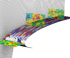
  $L=\{0.0021,0.01\}$, based on the chord length, were prescribed. The small integral length scale was selected in order to have similar conditions to the ones used in flat-plate simulations by Morra et al. (Reference Morra, Sasaki, Hanifi, Cavalieri and Henningson2019) and Brandt et al. (Reference Brandt, Schlatter and Henningson2004). While the use of a large length scale was selected to have conditions that are more likely to be found in experimental set-ups (see e.g. Fransson & Shahinfar Reference Fransson and Shahinfar2020). A snapshot of one of the simulations is presented in figure 2, where it can be seen the different disturbance behaviour inside and outside the boundary layer. Because of the use of different length scales, two different spectral element meshes were used, both structured and generated to be orthogonal to the wing surface. A summary of the domain and the FST generation conditions is presented in table 1. The three-dimensional meshes consist of 264 000 and 92 400 spectral elements for the cases with $L=0.01$ and $L=0.0021$, respectively. Note that the spanwise wavenumber resolution is defined by the extent of the span, being different for both meshes.

Figure 2. Snapshot of the flow field for the case ( $Tu=0.5\,\%$ and $L=0.01$). Pseudocolours represent the streamwise velocity perturbation. The streaks are visualised by selecting the isovolumes $u=\pm 0.01$.
Table 1. Summary of geometrical and flow parameters of cases under study.

Prior to the three-dimensional DNS calculations, the two-dimensional base flow computation was performed in Nek5000 for the two domains under consideration and using the Fluent results to retrieve the boundary conditions. In figure 3(a) the pressure distribution of the base flow for both meshes is shown, whereas figure 3(b) shows the streamwise velocity profiles at several chord locations. Here, it is also included the velocity profiles retrieved from the surface pressure distribution from DNS and by solving the boundary layer equations (BLEs) (see e.g. Schlichting & Gersten Reference Schlichting and Gersten2003). A good agreement for both quantities is observed, which indicates that the boundary layer in the DNS is well resolved and the base flow is unaltered under the mesh variation. Note that the operators in the LBLE in Appendix A are built considering the base flow obtained from the BLEs instead of the DNS since it does not require an interpolation nor a change of coordinates, leading to smoother derivatives.

Figure 3. Base flow comparison of domains used in cases 1–2 and cases 3–4 presented in table 1. (a) Pressure coefficient. (b) Streamwise velocity profiles  $U/U_\infty$ at different chord locations. The blue line corresponds to the boundary layer solver.
The normalised energy distribution of the FST generation is presented in figure 4(a) for both turbulent length scales. Figure 4(b) shows the turbulence intensity decay,  $Tu=\sqrt {(u_{rms}^{2} + v_{rms}^{2} + w_{rms}^{2})/3}$, with the chord for the four cases at different wall-normal directions, showing that a a reasonable level of homogeneity is reached. Moreover, a power-law fitting $Tu \propto (x-x_0)^{-c}$, with $c=0.6$ (Fransson et al. Reference Fransson, Matsubara and Alfredsson2005), is also included for validation of the turbulence intensity decay. As expected, there is a faster decay in turbulence intensity in the cases with the small turbulent scale.

Figure 4. (a) Energy distribution of the imposed FST as a function of the total wavenumber. (b) Turbulence intensity along the chord for the four cases at four different wall-normal locations ( $n/\delta ^{*}_{x=0.35}=8,10,12,14$). Normal position increases from grey to black. Markers, same as in (a), represent the power law fitting.
Due to the periodicity along the span  $z$, the integral length scale $L_{11}$ is computed in front of the leading edge using the longitudinal autocorrelation for the spanwise velocity $w$. The theoretical value for $L_{11}$, using (2.5), and the value computed from the autocorrelation are listed in table 1. For all cases the spanwise extension of the domain is greater than six times the integral length scale, which has been shown to be a reasonable lower limit to resolve the scales (O'Neill et al. Reference O'Neill, Nicolaides, Honnery and Soria2004).
4. Results
We start our investigation by analysing the response of the boundary layer to the different FST conditions from our DNS simulation. Then, the observed differences are explained by means of optimal disturbance theory.
4.1. Statistics in the boundary layer
Statistical results are computed by taking the average of the flow fields in time and along the periodic direction  $z$. Similarly to most of the findings in flat plate experiments, the increase in length scale in the FST results in a higher disturbance growth inside the boundary layer, and actually leading to transition for the high $Tu$ case. This can be seen in figure 5, where the maximum $u_{rms}$ along the wall-normal direction is shown for the four cases. For both turbulence intensities it is possible to observe a difference in growth when varying the turbulence length scale. The cases with small $L=0.0021$ show a peak in the $u_{rms}$ close to the leading edge, and decaying disturbances downstream. While the cases with large $L=0.01$ keep growing with the chord, even for the low $Tu$ simulation.

Figure 5. (a) Maximum wall-normal  $u_{rms}$ inside the boundary layer; lines are normalised by their corresponding turbulence intensity. (b) Skin friction coefficient along the chord.
The friction coefficient is also displayed in figure 5 since it is good measurement to define the onset of transition. Only the black line, corresponding to the case with large  $L$ and high $Tu$, shows an increase in the friction coefficient within our computational domain, which is in agreement with the fast growth in the $u_{rms}$ amplitude.
The wall-normal distribution of  $u_{rms}$ at different chord locations is displayed in figure 6 for the four cases. From these velocity profiles it is also possible to observe the decay and growth of the disturbances for the cases with small and large length scale, respectively. In particular, the peak of the profile in figure 6(d) gets closer to the wall at downstream locations, which is also an indication of transition to turbulence. This behaviour was also observed by Matsubara & Alfredsson (Reference Matsubara and Alfredsson2001).

Figure 6. Wall-normal distribution of  $u_{rms}$. Streamwise position increases from blue to red.
It is worth noting that despite the difference in the disturbance growth for the two turbulence length scales, streaky structures are triggered inside the boundary layer in all cases. An explanation for the different evolution of the streaks will be discussed later in this paper.
4.2. Turbulent spots
In this section, we analyse the nucleation of turbulent spots for the case corresponding to  $Tu=3\,\%$ and $L=0.01$, which is our only case where they can be found within the domain. Here, we aim to show that the same transition mechanisms present in flat plate configurations can be found in this geometry, where leading edge and pressure gradient effects are present.
This analysis is done by tracing back turbulent spots in the saved snapshots of the whole flow field. The generation and evolution of the studied turbulent spots follow the same behaviour reported by several works that can be found in the literature for flat plates (see e.g. Matsubara & Alfredsson Reference Matsubara and Alfredsson2001; Brandt et al. Reference Brandt, Schlatter and Henningson2004; Nagarajan et al. Reference Nagarajan, Lele and Ferziger2007). From the leading edge, laminar streaks are generated in the boundary layer and grow downstream due to the lift-up effect. Localised perturbations evolve into patches of irregular motion, travelling downstream as a wave packet while growing in the stream and spanwise directions. In all turbulent spots studied in this case, they were initiated from a single low-speed streak pushed to the edge of the boundary layer. An example of the generation and evolution of a turbulent spot is displayed in figure 7, where figure 7(a,c,e,g,i,k) show the spanwise velocity perturbation while figure 7(b,d, f,h,j,l) show the streamwise velocity perturbation, in wall parallel and wall-normal views, respectively. This time sequence illustrates the main features described above and is a good representation of the evolution of the turbulent spots found in our simulations.

Figure 7. Evolution of turbulent spot generation in the boundary layer, with time increasing from (a,b) to (k,l). (a,c,e,g,i,k) Wall parallel view of the spanwise velocity perturbation, where dark and light areas represent negative and positive values, respectively. Light blue arrow follows the nucleation and development of the turbulent spot, where it can be noted its size increase along the span and streamwise directions. (b,d, f,h,j,l) Wall normal view of the streamwise velocity perturbation, where blue and red areas represent negative and positive values, respectively. Here, it can be noted how the turbulent spot is initiated from a low-speed streak lifted towards the edge of the boundary layer. The solid line corresponds to  $3\delta ^{*}$ and the vectors to the normal and streamwise velocities. Dash–dotted lines correspond to the views of the adjacent plot.
The visual inspection of the flow fields during the early stages of the turbulent spots generation shows a sinuous-like type of secondary instabilities (see Brandt & Henningson (Reference Brandt and Henningson2002) for reference), while no signs of varicose-like instability were found. Hence, we will focus our attention in the generation of the sinuous-like breakdown. In figure 8 are shown snapshots at the same time instant as in figure 7(c,d), when the turbulent spot is not fully formed yet. The wall-parallel close-up view of the streaks in figure 8(b) shows how a low-speed streak exhibits high-frequency spanwise oscillations. As it will be discussed in the next section, high-frequency perturbations are damped in the boundary layer and therefore not effective in creating streaky structures, while the secondary instability being initiated from a nonlinear interaction with high-frequency modes in the free stream. The wall-normal close-up view in figure 8(c) shows the formation of a streamwise vortex at only one side of the low-speed streak. It can also be observed how the shear in the wall-normal and spanwise direction is larger close to the edge of the boundary layer.

Figure 8. Nucleation of a turbulent spot from a secondary instability. Snapshots correspond to the same time instant in figure 7(c,d). (a) Wall parallel (top) and wall-normal (bottom) views. Colours show the streamwise perturbation, solid line represents  $3\delta ^{*}$, and the dash–dotted line the view in the adjacent plot. (b) Close-up wall-normal view of the streak. Vectors represent the stream and spanwise velocity perturbations. (c) Normal wall view at $x=0.15$.
4.3. Receptivity
The response of the boundary layer to the FST is analysed by means of a Fourier transform along the periodic direction  $z$ and time. Due to the need for long time series, frequency spectra are not commonly computed from DNS data. However, our integration time is long enough to achieve convergence (see Appendix B) and sheds some light on the response of the boundary layer to FST. Moreover, and given the finite domain size and periodicity along the span, we have discrete wavenumbers that are defined by the span length for the respective cases.
Figure 9 shows the spectra of the streamwise velocity perturbation, as in (2.6), corresponding to the cases with  $L=0.0021$ at several chord locations and at a wall-normal location equal to $n=1.5\delta ^{*}$, with $\delta ^{*}$ being the local displacement thickness. Similarly, figure 10 presents the spectra for the cases with $L=0.01$. As was shown in figure 4(a), the FST spectrum for the cases with larger length scale have a higher energy content for lower total-wavenumbers. This difference in the FST boundary condition, together with the fact that the spanwise wavenumber resolution is dictated by the span length, results in a spectrum with more energetic modes at lower frequencies/wavenumbers for the cases corresponding to $L=0.01$ compared with the cases with $L=0.0021$. For this reason, the range of the contour plots in figure 10 is reduced to 60 % in both axis with respect to figure 9 for better visualisation. The numbers in the contour plots are labels for specific Fourier modes that will be analysed later in this work. An important characteristic of these Fourier modes is that they are part of the synthesised FST spectrum displayed in figure 4(a). The cases with low turbulence intensity, $Tu=0.5\,\%$, in figures 9 and 10 present a linear development of the incoming free stream disturbances, where the peaks in the spectra inside the boundary layer are part of the inlet FST boundary condition, while no other significant frequencies appear. Moreover, an extra case with $Tu=0.25\,\%$ and $L=0.01$ was run to confirm the linear receptivity of the boundary layer to low FST intensities. The results are presented in figure 11, showing the development of the wall-normal maximum $u_{rms}$ along the chord for $Tu=0.5\,\%$ and $Tu=0.25\,\%$ with and without normalisation by the turbulence intensity. When the curves are normalised by $Tu$ they collapse together with a maximum relative error of $\approx$3 %.

Figure 9. Spectrum for cases with  $L=0.0021$ at different chord locations and a wall-normal distance of $1.5\delta ^{*}$. The colours correspond to the streamwise velocity perturbation. Note that both axes in the contour plots in figure 10 are reduced to 60 % with respect to the ones presented in this figure for better visualisation. Here (a) $Tu=0.5\,\%$ and (b) $Tu=3\,\%$.

Figure 10. Spectrum for cases with  $L=0.01$ at different chord locations and a wall-normal distance of $1.5\delta ^{*}$. The colours correspond to the streamwise velocity perturbation. Note that both axes in the contour plots are reduced to 60 % of the ones in figure 9 for better visualisation. Here (a) $Tu=0.5\,\%$ and (b) $Tu=3\,\%$.

Figure 11. Development of maximum wall-normal  $u_{rms}$ along the chord without (a) and with (b) normalisation by turbulence intensity. Dashed line corresponds to $Tu=0.5\,\%$ and $L=0.01$ and dash–dotted line to $Tu=0.25\,\%$ and $L=0.01$.
On the other hand, when the turbulence intensity is increased, new frequencies, that were not present in the FST, appear inside the boundary layer due to nonlinear interactions. However, and especially for the low wavenumbers, the principal peaks are also coming from the FST, indicating that the linear receptivity mechanism (Brandt, Henningson & Ponziani Reference Brandt, Henningson and Ponziani2002) is still present and important for the high turbulence cases.
The results herein support the findings reported by Westin et al. (Reference Westin, Bakchinov, Kozlov and Alfredsson1998), and more recently in the investigation of Fransson & Shahinfar (Reference Fransson and Shahinfar2020), that the scales of the FST play an important role on the scale of the induced streaks. In particular, for our low turbulence intensity simulations the scale of the streaks is already set in the incoming free stream vorticity, and the differences in the growth that these Fourier modes experience will be explained in the next section by means of optimal disturbances.
However, when the turbulence intensity increases and given the appearance of nonlinear interactions, a definite statement is harder to make. Brandt et al. (Reference Brandt, Henningson and Ponziani2002) pointed out that linear and nonlinear mechanisms could indeed cooperate and interact, and the dominance of one or the other would depend on the amount of energy in the low-frequency part of the spectrum. This seems to be consistent with our results for the cases with high turbulence intensity. Here, the case with  $L=0.01$, having higher energy content in low frequencies, is the only case that undergoes transition within our domain. Moreover, as it will be shown in the next section, in this case the Fourier modes show a higher deviation from linear theory.
4.4. Optimal growth
We now study the optimal transient growth of disturbances by solving the LBLE (Andersson et al. Reference Andersson, Berggren and Henningson1999; Luchini Reference Luchini2000) and following the method described in Appendix A. Our main goal here is to explain the observed differences in growth when changing the turbulence length scale. As mentioned before, the base flow is obtained from the BLEs instead of the two-dimensional DNS simulations. The pressure distribution at the airfoil surface is retrieved from the DNS base flow calculations and used to compute the velocity field, as it was shown in figure 3(b). This kind of approach, instead of using the whole DNS base flow, has been proved to give good results in previous works (see e.g. Tempelmann et al. Reference Tempelmann, Schrader, Hanifi, Brandt and Henningson2012) and also in the present investigation.
We are interested in understanding the dependency of the optimal growth on the spanwise wavenumber  $\beta$ and the frequency $\omega$. Thus, the optimisation algorithm described in Appendix A is performed for different values of $\beta$ and $\omega$ by finding the optimal growth at several final locations $x_f$. A summary of the results are presented in the contour plots of figure 12, where the isolines represent the envelope of the maximum $|\hat {u}(\beta )|$ in the wall-normal direction and the dashed lines the wavenumber experiencing maximum transient growth at each $x$ location. These contour plots were generated considering the initial location for the optimal perturbation equal to $x_0=0.005$. Different $x_0$ may give higher growth rates, as was shown in Levin & Henningson (Reference Levin and Henningson2003). However, in the present study we are mainly interested in the growth variations with respect to the frequency and wavenumber. And despite the dependency on the initial location $x_0$, the general trend remains unchanged and the same conclusions can be drawn.

Figure 12. Contour plots of maximum transient growth for selected frequencies. The dashed line corresponds to the wavenumber  $\beta$ with maximum transient growth at the given chord location. Here (a) $\omega =0$, (b) $\omega =10$ and (c) $\omega =20$.
By comparing the contour plots for different frequencies in figure 12, it can be noted that low-wavenumber and low-frequency waves can experience higher transient growth. In particular, maximum transient growth within our domain is attained for steady streaks ( $\omega =0$), and as can be seen in the sequence of contour plots in figure 12, this growth decreases once the streak frequency increases. This is also consistent with the behaviour of optimal perturbations over flat plates (Andersson et al. Reference Andersson, Berggren and Henningson1999; Luchini Reference Luchini2000) and the coupling coefficient (Zaki & Durbin Reference Zaki and Durbin2005), which describes the effectiveness of a particular mode to penetrate the boundary layer and generate streaks. The effect of increasing frequency in figure 12 is interesting, even though it overall reduces the disturbance growth, its effect is larger for the low wavenumber region. For these larger structures, the growth is significantly decreased downstream, while high wavenumbers can still experience their high growth close to the leading edge with little variation. Consequently, the wavenumber experiencing maximum growth at downstream locations shifts towards higher values when the frequency is increased, as it can be noticed by comparing the dashed lines in the contour plots of figure 12.
The preference of the boundary layer to low frequencies and wavenumbers is consistent with the differences in growth observed in figure 5 for the  $u_{rms}$, where our synthesised inlet spectrum with larger turbulence length scale $L$ contains lower wavenumbers and frequencies. Evidence of this behaviour can also be found, for instance, in Jacobs & Durbin (Reference Jacobs and Durbin2001) and Westin et al. (Reference Westin, Bakchinov, Kozlov and Alfredsson1998). However, it has to be noted that the synthesised spectrum from Jacobs & Durbin (Reference Jacobs and Durbin2001) did not contain the low frequencies that appeared downstream in their simulation, which were attributed to the result of nonlinear interactions.
The fact that large wavenumbers can experience a significant growth close to the leading edge almost independent of their frequency can qualitatively explain some features of our DNS results presented in the previous section (see figure 5). There, our cases with small  $L$, having their energy distributed over higher frequencies and wavenumbers, showed a significant growth close to the leading edge to then decay. A similar observation was made by Brandt et al. (Reference Brandt, Schlatter and Henningson2004) for their case with smallest scales (cf. figure 4a). Their conjecture was that the boundary layer has a high receptivity for high frequencies close to the leading edge, but the growth cannot be sustained because of the faster decay of the FST for small scales, and therefore is less effective in continuously forcing the disturbances inside the boundary layer (Westin et al. Reference Westin, Bakchinov, Kozlov and Alfredsson1998). However, the optimal disturbance computation does not consider any effect from the continuous forcing while still being able to qualitatively explain the trend for the different scales observed in our simulations. A quantitative comparison between optimal growth and our DNS results will be discussed in the next section to strengthen this point.
4.4.1. Comparison with DNS
In the previous section we showed a qualitative agreement between optimal growth and our DNS results. In this section we move to a quantitative comparison by comparing the growth of the spatiotemporal Fourier modes  $(\omega,\beta )$ with the linear theory and the optimal growth.
The comparison with linear theory is carried out by extracting the DNS disturbance at some location  $x_0$ close to the leading edge, and using this profile as an initial condition in the direct LBLE calculation for the Fourier modes of interest. In order to satisfy the boundary condition in the free stream, the velocity profiles are damped using a step function of the form
 \begin{equation} S(n) =
\left\{\begin{array}{@{}ll} 0, & n \geq n_{max}\\
1\left/\left[1+\exp \left(\dfrac{n_{max}-n_{dm}}{n_{max}-n}
+ \dfrac{n_{max}-n_{dm}}{n_{dm}-n} \right) \right] \right.
, & n_{dm}< n < n_{max}\\ 1, & n \leq n_{dm}
\end{array}\right. \end{equation}
\begin{equation} S(n) =
\left\{\begin{array}{@{}ll} 0, & n \geq n_{max}\\
1\left/\left[1+\exp \left(\dfrac{n_{max}-n_{dm}}{n_{max}-n}
+ \dfrac{n_{max}-n_{dm}}{n_{dm}-n} \right) \right] \right.
, & n_{dm}< n < n_{max}\\ 1, & n \leq n_{dm}
\end{array}\right. \end{equation}
where  $n_{max}$ corresponds to the maximum wall-normal coordinate and $n_{dm}$ the wall-normal distance from where the damping is performed. The results presented below were generated considering $n_{dm}\approx 90\delta ^{*}$ and $n_{dm}\approx 180\delta ^{*}$ for the cases with small and large turbulent length scale $L$, respectively. Note that smaller wavenumbers have to be damped at higher distances from the wall to achieve convergence of the linear solution, which is consistent with the fact that optimal disturbances take longer to decay to zero in the free stream when decreasing the wavenumber.
The comparison with optimal growth is performed by extracting the DNS Fourier modes  $(\omega,\beta )$ close to the leading edge, but in this case the mode is projected onto the optimal disturbance in order to obtain the energy that corresponds to the optimal and thereby used as scaling factor. The steps for the projection for a given $(\omega,\beta )$ are listed below.
(i) Select an initial location $x_0$. At this position the DNS profile is extracted and denoted as $\boldsymbol {\hat {q}}_{DNS}$ in the following. This position is also used as the location of the optimal initial disturbance.
(ii) Select a final location
$x_f$. At this position the maximum transient growth is maximised by finding the optimal initial disturbance $\boldsymbol {\hat {q}}_0$.(iii) Project the DNS profile
$\boldsymbol {\hat {q}}_{DNS}$ over the optimal perturbation $\boldsymbol {\hat {q}}_0$. This is done by using the inner product associated with the norm in the space of disturbance (see (2.7)) and reads
(4.2)The subscript\begin{equation} a_{f} = \langle \boldsymbol{\hat{q}}_{0},\boldsymbol{\hat{q}}_{DNS} \rangle = \frac{1}{2} \int \boldsymbol{\hat{q}}_{0}^{H}\boldsymbol{\hat{q}}_{DNS}\,\mathrm{d}n. \end{equation}$f$ is included to emphasise that the projection is performed for the initial optimal disturbance that maximises the energy at $x_f$.(iv) Scale the optimal growth. Using (2.7), the optimal disturbances are computed considering unitary initial energy
$E(\boldsymbol {\hat {q}}_0)=1$. Hence, and to properly compare with DNS, the square root of the energy corresponding to the projection over the optimal is used as scaling factor
(4.3a)\begin{align} E_{proj} &= \langle a_{f}\boldsymbol{\hat{q}}_0,a_{f}\boldsymbol{\hat{q}}_0\rangle \end{align}(4.3b)\begin{align} &= |a_{f}|^{2} E(\boldsymbol{\hat{q}}_0) \end{align}(4.3c)\begin{align} &= |a_{f}|^{2}. \end{align}(v) The process is repeated from step (ii) for different
$x_f$ locations.


Figure 13 illustrates how this projection is performed. Figure 13(a) show the velocity profiles at  $x_0$ for the DNS and the optimal without and with scaling. Note that the optimal initial disturbance correspond to a single optimal response at $x_f$. Figure 13(b,c) show the comparison between DNS and the scaled optimal growth. The yellow lines correspond to the DNS results, while the grey lines to the scaled optimal growth. The stars in the $|\hat {u}|_{max}$ plot represent not only the velocity peak, but also the location $x_f$ where the transient growth was maximised for each grey line.

Figure 13. Example of the projection over the optimal disturbance for Fourier mode labelled as 3 in figure 9. (a) Input from DNS and the unscaled and scaled optimal disturbance at  $x_0$. (b) Response at $x_f$ from DNS and scaled optimal. (c) Development of the maximum streamwise perturbation with the chord.
In the study of Andersson et al. (Reference Andersson, Berggren and Henningson1999), it was shown how the shape of experimental  $u_{rms}$ profiles follow the shape of the optimal response. Similarly, shape comparisons with numerical experiments can be found, for instance, in Brandt et al. (Reference Brandt, Schlatter and Henningson2004) and Nagarajan et al. (Reference Nagarajan, Lele and Ferziger2007). In the present work, and by looking at the outputs in figure 13, it can be noticed how the projection over the optimal not only recovers the shape of the response as a streak, but also its amplitude. Obviously, in this case we are comparing a specific mode instead of the total $u_{rms}$, but as it was shown by Luchini (Reference Luchini2000), the shape of the optimal response is very insensitive to wavenumber variations. Therefore, it is not surprising that the $u_{rms}$, which is the combination of all modes, resembles the optimal shape too.
The optimisation algorithm requires a fixed final location  $x_f$ where maximum growth is sought. This is represented by the different grey lines in figure 13(c). It is not until we perform the projection for optimal corresponding to several chord locations that we can retrieve the development of the Fourier mode along the chord, which evidences how, at each chord location, an arbitrary disturbance will grow according to its projection onto the optimal.
The same procedure described above was performed for different  $(\omega, \beta )$ pairs for our four cases. The modes were selected according to their amplitude inside the boundary layer in the low turbulence intensity cases. In figures 9 and 10, the Fourier modes to be analysed with their respective numbering are shown. Note that a fixed $x_0$ has to be specified to perform the projection, even when receptivity is a non-local process. For this reason, different initial positions $x_0$ were considered in a distance of 1 %–4 % of the chord from the leading edge. Some of these results are included in Appendix C. Varying the initial optimal disturbance location within this range did not change significantly the optimal growth, showing the following analysis being independent of our arbitrary choice for $x_0$.
Figures 14 and 15 show the comparison of the Fourier modes growth from the DNS calculations, linear theory and projection over the optimal, for the cases with small and large turbulent scales, respectively. The low turbulence intensity cases present an excellent agreement between DNS results and linear theory. And since we are extracting the velocity profile close to the leading edge, this close agreement indicates that receptivity to FST takes place in this region and subsequently evolve due to linear mechanism. When the turbulence intensity is increased to 3 %, there is still a remarkable similarity between the DNS and linear theory growth, particularly for the case with  $L=0.0021$, in figure 14, and in the initial section of the wing for the case with $L=0.01$, in figure 15. For the latter case, a comparison with linear theory after $x\approx 0.15$ is not relevant due to the presence already of turbulent spots at those chord locations (see figure 7). Here, and for most of these Fourier modes, linear theory overpredicts their growth, showing that energy is being transferred from these modes. This poorer agreement between linear theory and DNS for the high turbulence intensity cases is not surprising given the results shown in figures 9 and 10, where was already depicted the nonlinear response of the boundary layer to the incoming FST.

Figure 14. Growth of different modes  $(\omega,\beta )$ corresponding to $L=0.0021$. Colour lines represent DNS data, dashed lines projection over the optimal and solid black lines LBLE results using DNS profile as initial condition. See figure 9 for modes numbering. Here (a) $Tu=0.5\,\%$ and (b) $Tu=3.0\,\%$.

Figure 15. Growth of different modes  $(\omega,\beta )$ corresponding to $L=0.01$. Colour lines represent DNS data, dashed lines projection over the optimal and solid black lines LBLE results using DNS profile as initial condition. See figure 10 for modes numbering. Here (a) $Tu=0.5\,\%$ and (b) $Tu=3.0\,\%$.
The dashed lines in figures 14 and 15 correspond to the scaled optimal growth described above and sketched in figure 13, but here only the values at the final optimised locations are shown (the stars in figure 13). From these plots it can be seen that for the low turbulence intensity cases there is a good agreement between the projection over the optimal and the DNS results. In particular, the growth of all Fourier modes for the case with small  $L$ in figure 14 is properly captured in terms of their evolution and amplitude along the chord. This is true despite the distinct evolution of the modes, and even when in some cases the only change is the frequency for a given wavenumber, as is the case for modes $\{1,2,5,6\}$, $\{3,7\}$ and $\{4,8\}$. For the case with large $L$ in figure 15, there is also a good agreement for most of their modes, being also able to capture the different evolution that the modes undergo. However, a bigger mismatch for the lowest wavenumber $\beta \approx 90$ (modes $\{1,2,6,7\}$) can also be observed, especially the over-prediction for mode $7$.
$7$.
In figures 14 and 15 the optimal growth for the cases with high turbulence intensity is also reported. For these cases, there is a more pronounced difference between optimal growth and the DNS Fourier modes, especially for the case with larger  $L$ (see figure 15). However, these differences are expected given the already mentioned mismatch with respect to linear theory.
Optimal disturbances are obtained from an initial-value problem describing the downstream evolution of an initial perturbation, without including the effect of any type of continuous forcing of the free stream on the boundary layer. Therefore, the good agreement between optimal theory and DNS implies that the differences in perturbation growth observed in the DNS for different integral length scales are not due to the FST decay rate, but to the apparent property of the boundary layer in amplifying individual frequencies and wavenumbers. Furthermore, this amplification, for a given arbitrary initial disturbance, will be given by its projection onto the optimal.
5. Discussion
In this section we address some of the questions that have arisen due to the close agreement between the optimal perturbation computations and DNS for most of the Fourier modes, and the mismatch of some of them.
5.1. Optimal growth from arbitrary perturbations
A possible explanation for the good agreement between DNS results and optimal perturbations is that the initial perturbations at the leading edge are already very close to the optimal. To examine this possibility we need to quantify how much of the arbitrary DNS initial perturbations correspond to the optimal disturbances.
This is measured as the ratio between the projection coefficient  $a_f$, given in (4.2), and the energy of the DNS profile at $x_0$. This ratio is calculated for each pair $(\omega,\beta )$ and for the optimal initial disturbance that maximises the energy at a given $x_f$:
 \begin{equation} \mathcal{E}_{(\omega,\beta)}(x_f) = \left.\frac{|a_{f}(\omega,\beta)|}{\sqrt{E_{DNS}(\omega,\beta)}}\right., \end{equation}
where  $E_{DNS}$ is computed using the norm defined in (2.7) and $n_{max}$ is chosen as the wall-normal location where the optimal initial disturbance satisfies $\boldsymbol {q}^{H}_{0}\boldsymbol {q}_{0} |_{n_{max}} \approx 0$. This is because the FST is still present as $n\to \infty$ and we want to account solely for the part of the disturbance that can be projected onto the optimal. The computation of this quantity is justified by the orthogonality of the right singular vectors of the operator $\mathcal {A}$ in (2.8). Here, the energy of the singular vectors is additive, while the first right singular vector corresponds to the optimal disturbance when the singular values are sorted in decreasing order.
The ratio in (5.1) is then computed for every Fourier mode and projection, obtaining values ranging within 10 %–50 % while no correlation between the agreement with DNS and the quantity  $\mathcal {E}$ was found. This result thus rules out the hypothesis that the Fourier modes are already optimal, and the good correspondence between optimal and DNS seems to be independent of how ‘similar’ they are. Moreover, it confirms that the optimal is the main component of the disturbance that leads to transient growth, something that was already pointed out in the early optimal disturbance investigations and in concordance with the fast convergence of the power iterations found here and previous works (Andersson et al. Reference Andersson, Berggren and Henningson1999; Luchini Reference Luchini2000; Levin & Henningson Reference Levin and Henningson2003). In fact, Luchini (Reference Luchini2000) showed that the second singular value of the evolution operator was already around three orders of magnitude smaller than the first one.
From the considerations mentioned above, it is then not surprising that the shape of the boundary layer response to randomly synthesised or general grid turbulence tends to the optimal even when optimal perturbations have never been observed in experiments. However, there is a natural follow-up question to this claim. If the growth is dictated by the optimal, why the big mismatch for mode 7 in figure 15? In the following section, we summarise our efforts to find the cause of this discrepancy and what we think is the most likely reason.
5.2. The effect of the streamwise perturbation
There are a few uncertainties in our procedure that can be sources of error and account for the small deviation of the linear and optimal theory from the DNS for the low  $Tu$ cases. First, all our DNS simulations are nonlinear, so even though we can categorise them as linear, this is an a posteriori result and the fact that small nonlinearities can still be present is unavoidable. Secondly, the Fourier modes were computed by taking the Fourier transform of a non-periodic signal in time, which will always cause spectral leakage. However, we show in Appendix B that a good level of convergence is achieved with the length of our signal, and the dominant frequencies are captured independent of the windowing function. Finally, to perform the projection we are forced to select a specific initial location, even when receptivity is a non-local phenomenon. The influence of this arbitrary $x_0$ choice was evaluated but its effect was found to be small, as is shown in Appendix C. With that being said, the optimal growth of the Fourier mode labelled as 7 in figure 15 has consistently mismatched the DNS results, independent of the chosen initial location $x_0$, length of the time series, windowing function, and despite the close agreement with linear theory.
After discarding the aforementioned sources of error that could be responsible for the clear mismatch, we can conjecture that the most likely cause for the disagreement is the large initial streamwise velocity  $u$ that this particular Fourier mode has, as it can be seen in figure 15 around $x=0$. This large streamwise velocity makes the initial perturbation very different from the distinctive optimal perturbation shape, which takes the form of a counter-rotating streamwise vortex. Besides, this explanation seems to be consistent with the observation made in by Luchini (Reference Luchini2000) and the vortex receptivity study by Schrader et al. (Reference Schrader, Brandt, Mavriplis and Henningson2010).
Luchini (Reference Luchini2000) (cf. Appendix B) addresses the question of whether disturbances with streamwise velocity component  $u$ can be amplified or not. He concludes that if there is a coupling between the initial streamwise velocity perturbation and initial streamwise vorticity perturbation, then amplification of $u$ is possible. However, he also concludes that damped perturbations exist and they are the combination of a $u$ profile and a suitable streamwise vortex, which can also be seen as a rotated wall-normal vorticity. Similarly, an optimal streamwise vortex can be rotated, by the effect of the streamwise velocity perturbation, and still experience its optimal growth.
In our simulations, the disturbances are generated to be randomly oriented as long as continuity is satisfied. Therefore, the good agreement between optimal and DNS for most of the Fourier modes seems, at first glance, unlikely. According to Luchini (Reference Luchini2000), this can be explained by the high probability of a random perturbation to be oriented in a way that it contains a significant fraction of the streamwise vorticity. Moreover, the leading edge is able to convert the normal incoming vorticity into streamwise vorticity through stretching and tilting (Goldstein et al. Reference Goldstein, Leib and Cowley1992). And as it was shown by Schrader et al. (Reference Schrader, Brandt, Mavriplis and Henningson2010), this conversion is more effective for large wavenumbers, which are actually the Fourier modes in our simulations where the best agreement can be found. On the other hand, the mode that has been labelled as 7 in figure 15 corresponds to the lowest spanwise wavenumber that can be solved in our domain. Therefore, the leading edge is not as effective in converting its high streamwise velocity amplitude into a streamwise vortex. Although not shown here, the modal content of the vorticity in front of the leading-edge was analysed, showing a dominant normal component for mode 7 and in consistency with its large initial streamwise velocity perturbation.
6. Conclusions
In the present work, we have investigated the receptivity and response of the boundary layer over a wing profile to FST by means of DNS. In particular, four different FST conditions have been studied, considering two different length scales under low and high turbulence intensities. In all studied cases, the disturbances inside the boundary layer develop into streaky structures of alternating high and low streamwise velocity, with only one of the cases showing signs of the onset to transition within our computational domain. The development of the disturbances inside the boundary layer was compared with linear theory and non-modal optimal disturbances in the high Reynolds limit.
The cases with low turbulence intensity presented a linear receptivity to the incoming FST. In particular, the amplitude of Fourier modes inside the boundary layer, for most cases, can be predicted by the projection of the arbitrary disturbance over the optimal ones. This indicates that the optimal transient growth is the main mechanism behind the disturbance evolution observed in our simulations. To the best of the authors’ knowledge, this is the first time an explicit comparison between optimal and randomly generated disturbances is performed, strengthening the relevance of the optimal disturbance in the study of FST-induced perturbations.
Moreover, the study of the Fourier modes growth supports the thesis that the scales of the free stream vorticity play a fundamental role in the induced streaks. This does not contradict the existence of preferred spanwise wavenumbers that can exhibit maximum transient growth; they exist and can be determined by optimal disturbance theory. In fact, the existence of preferred spanwise wavenumbers explains the observed differences in our cases when the length scale was changed. Our results also suggest that receptivity to low levels of FST takes place in a region around the leading edge and the generated perturbations then grow according to their projection over the optimal, without considering any continuous forcing from FST. However, when the turbulence intensity increases, nonlinear interactions become important and the growth of Fourier modes deviates from linear theory.
Finally, the transition to turbulence was studied by tracing back the nucleation of turbulent spots from the visual inspection of the saved flow fields. Our case where the onset of transition was observed showed the same turbulent spot development that has previously been reported in several flat plate experiments and simulations. Here, a secondary instability was triggered after that a low-speed streak was lifted towards the boundary layer edge, and only sinuous-like instabilities were observed.
Funding
This work was funded by Vinnova through the NFFP project LaFloDes, with grant number 2019-05369, the European Research Council under grant agreement 694452-TRANSEP-ERC-2015- AdG and the Swedish e-Science Research Centre (SeRC). The computations were performed on resources provided by the Swedish National Infrastructure for Computing (SNIC) at NSC and PDC.
Declaration of interests
The authors report no conflict of interest.
Appendix A
In our formulation, the BLEs are linearised around a two-dimensional and steady base flow  $(U(s,n),V(s,n),0)$. Then the LBLE can be expressed in operator form
 \begin{equation} \mathcal{L}\hat{\boldsymbol{q}}=0, \end{equation}
where  $\mathcal {L}$ is a linear operator
 \begin{equation} \mathcal{L} = \boldsymbol{\mathsf{A}} + \boldsymbol{\mathsf{B}}\frac{\partial}{\partial n} + \boldsymbol{\mathsf{C}}\frac{\partial^{2}}{\partial n^{2}} + \boldsymbol{\mathsf{D}}\frac{1}{h_1}\frac{\partial}{\partial s}. \end{equation}
And the individual linear operators, for our formulation, take the form
 \begin{gather} \boldsymbol{\mathsf{A}} = \begin{bmatrix} 0 & m_{13} & \mathrm{i}\beta & 0 \\ \dfrac{1}{h_1}\dfrac{\partial U}{\partial s} -\mathrm{i}\omega + \dfrac{\beta^{2}}{\mbox{Re}} & \dfrac{\partial U}{\partial n}+ m_{13}U & 0 & 0 \\ \dfrac{\partial V}{\partial s} -2m_{13}U & \dfrac{1}{h_1} \dfrac{\partial V}{\partial n} -\mathrm{i}\omega + \dfrac{\beta^{2}}{\mbox{Re}} & 0 & 0 \\ 0 & 0 & -\mathrm{i}\omega + \dfrac{\beta^{2}}{\mbox{Re}} & \mathrm{i}\beta \end{bmatrix}, \end{gather}
 \begin{gather} \boldsymbol{\mathsf{B}} = \begin{bmatrix} 0 & 1 & 0 & 0\\ V & 0 & 0 & 0\\ 0 & V & 0 & 1\\ 0 & 0 & V & 0 \end{bmatrix}, \end{gather}
 \begin{gather} \boldsymbol{\mathsf{C}} = \begin{bmatrix} 0 & 0 & 0 & 0\\ -\dfrac{1}{\mbox{Re}} & 0 & 0 & 0\\ 0 & -\dfrac{1}{\mbox{Re}} & 0 & 0\\ 0 & 0 & -\dfrac{1}{\mbox{Re}} & 0 \end{bmatrix}, \end{gather}
 \begin{gather} \boldsymbol{\mathsf{D}} = \begin{bmatrix} 1 & 0 & 0 & 0\\ U & 0 & 0 & 0\\ 0 & U & 0 & 0\\ 0 & 0 & U & 0 \end{bmatrix}. \end{gather}
 The terms  $h_1$ and $m_{13}$ come from the use of the curvilinear coordinates following the airfoil profile. They are defined in terms of the curvature $\kappa$:
 $$\begin{gather} \kappa = \frac{|x'y'' - y'x''|}{(x'^{2}+y'^{2})^{3/2}}, \end{gather}$$
 $$\begin{gather}h_1 = 1 + n\kappa, \end{gather}$$
 $$\begin{gather}m_{13} = \frac{\kappa}{h_1}, \end{gather}$$
where  $(x,y)$ are the airfoil coordinates in Cartesian coordinates and primes define derivatives with respect to $s$. Using the LBLE, we want to find the initial perturbation which gives the maximum energy at a given downstream location of interest. Adopting an input–output formulation with the LBLE being our system of interest, we study the development of the output $\hat {\boldsymbol {q}}_{out}=\hat {\boldsymbol {q}}(s_{f})$ for a given input $\hat {\boldsymbol {q}}_0=\hat {\boldsymbol {q}}(s_{0})$:
 \begin{equation} \hat{\boldsymbol{q}}_{out} = \mathcal{A}\hat{\boldsymbol{q}}_0, \end{equation}
where  $\mathcal {A}$ is a linear operator. Here, operator $\mathcal {A}$ is defined through (A1). A common measure for the magnitude of a disturbance at some streamwise location is its kinetic energy defined in (2.7). The optimal disturbance is then calculated by finding the input at $s_0$, with unit energy $E_0=1$, that maximises the output energy at some final location $s_f$. In the limit for high Reynolds numbers, further simplifications can be made by considering inputs with zero streamwise velocity component, and outputs with streamwise velocity component only (see, for instance, Andersson et al. (Reference Andersson, Berggren and Henningson1999) for details). This formulation allows us to write explicitly the norms for inputs and outputs as
 $$\begin{gather} \|\hat{\boldsymbol{q}}_0 \|^{2} = \frac{1}{2}\int_{0}^{n_{max}} (\overline{\hat{v}}_0\hat{v}_0+ \overline{\hat{w}}_0\hat{w}_0) \mathrm{d}n, \end{gather}$$
 $$\begin{gather}\|\hat{u}_f \|^{2} = \frac{1}{2}\int_{0}^{n_{max}} \overline{\hat{u}}_f\hat{u}_f\,\mathrm{d}n, \end{gather}$$
with the bar representing the complex conjugate for scalar fields. Following these assumptions, the maximisation problem is reduced to find the maximum spatial transient growth  $G(s_f)$:
 \begin{equation} G(s_f) = \max_{\hat{\boldsymbol{q}}_0\neq 0} \frac{||\hat{u}_f ||^{2}}{||\hat{\boldsymbol{q}}_0 ||^{2}} = \max_{\hat{\boldsymbol{q}}_0\neq 0} \frac{\left\langle \mathcal{A}\hat{\boldsymbol{q}}_0, \mathcal{A}\hat{\boldsymbol{q}}_0\right\rangle}{\left\langle\hat{\boldsymbol{q}}_0, \hat{\boldsymbol{q}}_0\right\rangle}. \end{equation}
The maximal is then given by the eigenvector corresponding to the largest eigenvalue of the generalised eigenvalue problem
 \begin{equation} \mathcal{A}^{*}\mathcal{A}\hat{\boldsymbol{q}}_0 = \lambda \hat{\boldsymbol{q}}_0, \end{equation}
where  $\mathcal {A}^{*}$ represents the adjoint of operator $\mathcal {A}$ with respect to the chosen inner product, while $\lambda _{max}$ corresponds to the maximum transient growth. Starting from an arbitrary initial condition, the eigenvector corresponding to the maximum eigenvalue can be computed through power iterations
 \begin{equation} \hat{\boldsymbol{q}}_0^{n+1}=\mathcal{A}^{*}\mathcal{A}\hat{\boldsymbol{q}}_0^{n}. \end{equation}
 To solve the power iterations we need to derive the adjoint system. By defining the inner product between two arbitrary functions  $\boldsymbol {u}$ and $\boldsymbol {v}$ as
 \begin{equation} (\boldsymbol{u},\boldsymbol{v}) = \int_{s_0}^{s_f}\int_{0}^{n_{max}} \boldsymbol{u}^{H} \boldsymbol{v}h_1 \,\mathrm{d}n \,\mathrm{d}s, \end{equation}
and the adjoint-state vector  $\boldsymbol {q}^{*}=(p^{*},u^{*},v^{*},w^{*})^{\rm T}$, we can then take the inner product between $\boldsymbol {q}^{*}$ and the system (A1) to find the associated adjoint operator. The derivatives are moved from the direct to the adjoint variables by integration by parts reading
 \begin{align} (\boldsymbol{q}^{*}, \mathcal{L}\hat{\boldsymbol{q}} ) &= \int_{s_0}^{s_f}\int_{0}^{n_{max}} (\boldsymbol{q}^{*})^{H} \left(\boldsymbol{\mathsf{A}} \boldsymbol{q} + \boldsymbol{\mathsf{B}}\frac{\partial \hat{\boldsymbol{q}}}{\partial n} + \boldsymbol{\mathsf{C}}\frac{\partial^{2} \hat{\boldsymbol{q}}}{\partial n^{2}} + \boldsymbol{\mathsf{D}}\frac{1}{h_1} \frac{\partial \hat{\boldsymbol{q}}}{\partial s} \right)h_1 \mathrm{d}n\,\mathrm{d}s \end{align}
 \begin{align} &= \int_{s_0}^{s_f}\int_{0}^{n_{max}} \left(\boldsymbol{\mathsf{A}}^{*} \boldsymbol{q}^{*} + \boldsymbol{\mathsf{B}}^{*} \frac{\partial \boldsymbol{q}^{*}}{\partial n} + \boldsymbol{\mathsf{C}}^{*}\frac{\partial^{2} \boldsymbol{q}^{*}}{\partial n^{2}} + \boldsymbol{\mathsf{D}}^{*}\frac{1}{h_1}\frac{\partial \boldsymbol{q}^{*}}{\partial s} \right)^{H} \hat{\boldsymbol{q}}h_1\,\mathrm{d}n\,\mathrm{d}s \nonumber\\ &\quad +\int_{s_0}^{s_f}\left[(\boldsymbol{q}^{*})^{H} \left(\boldsymbol{\mathsf{B}} - m_{13}\boldsymbol{\mathsf{C}} \right) \hat{\boldsymbol{q}} + (\boldsymbol{q}^{*})^{H}\boldsymbol{\mathsf{C}}\frac{\partial \hat{\boldsymbol{q}}}{\partial n} - \left(\frac{\partial \boldsymbol{q}^{*}}{\partial n}\boldsymbol{\mathsf{C}}\hat{\boldsymbol{q}} \right)^{H} \right]_{n=0}^{n=n_{max}} h_1\,\mathrm{d}s \nonumber\\ &\quad +\int_{0}^{n_{max}}\left[(\boldsymbol{q}^{*})^{H} \boldsymbol{\mathsf{D}}\hat{\boldsymbol{q}} \right]_{s=s_0}^{s=s_f}\,\mathrm{d}n, \end{align}
where
 $$\begin{gather} \boldsymbol{\mathsf{A}}^{*} = \boldsymbol{\mathsf{A}}^{H} - \frac{\partial \boldsymbol{\mathsf{B}}^{H}}{\partial n} - m_{13}\boldsymbol{\mathsf{B}}^{H} - \frac{\partial \boldsymbol{\mathsf{D}}^{H}}{\partial s}, \end{gather}$$
 $$\begin{gather}\boldsymbol{\mathsf{B}}^{*} ={-}\boldsymbol{\mathsf{B}}^{H} + 2 m_{13} \boldsymbol{\mathsf{C}}^{H}, \end{gather}$$
 $$\begin{gather}\boldsymbol{\mathsf{C}}^{*} = \boldsymbol{\mathsf{C}}^{H}, \end{gather}$$
 $$\begin{gather}\boldsymbol{\mathsf{D}}^{*} ={-}\boldsymbol{\mathsf{D}}^{H}. \end{gather}$$
The single integrals in (A14b) represent the boundary terms, corresponding to four integrals. Setting them equal to zero, and noting that the left-hand side in (A14a) is also zero, leads to the adjoint LBLE equations
 \begin{equation} \boldsymbol{\mathsf{A}}^{*} \boldsymbol{q}^{*} + \boldsymbol{\mathsf{B}}^{*}\frac{\partial \boldsymbol{q}^{*}}{\partial n} + \boldsymbol{\mathsf{C}}^{*}\frac{\partial^{2} \boldsymbol{q}^{*}}{\partial n^{2}} + \boldsymbol{\mathsf{D}}^{*}\frac{1}{h_1} \frac{\partial \boldsymbol{q}^{*}}{\partial s} = 0. \end{equation}
Zeroing the boundary terms also supplies the boundary conditions for the adjoint LBLE variables. The first three boundary terms, which are associated with the integral along the streamwise direction, define the necessary boundary conditions
 $$\begin{gather} \overline{u^{*}}=\overline{v^{*}}=\overline{w^{*}}=0\quad\mathrm{at } {n=0} , \end{gather}$$
 $$\begin{gather}\overline{u^{*}}=\overline{v^{*}}=\overline{w^{*}}=0\quad\mathrm{at } {n=n_{max}} . \end{gather}$$
While zeroing the fourth term supplies the initial condition
 $$\begin{gather} U(n) u^{*}(n) + p^{*}(n) = \hat{u}(n) \quad \mathrm{at } s=s_f, \end{gather}$$
 $$\begin{gather}v^{*}(n) = w^{*}(n) = 0 \quad\mathrm{at } s=s_f \end{gather}$$
and the action of the adjoint
 $$\begin{gather} \hat{v}(n) = U(n)v^{*}(n) \quad \mathrm{at } s=s_0, \end{gather}$$
 $$\begin{gather}\hat{w}(n) = U(n)w^{*}(n) \quad \mathrm{at } s=s_0. \end{gather}$$
Appendix B
The computation of frequency spectra from DNS data requires the use of long enough time series in order to avoid inaccuracies associated with the frequency resolution, which are especially detrimental for low frequencies. Another reason for the need of long time series is the fact that the signals are not exactly periodic in time, and the use of a long-time integration can help to avoid some of the spectral leakage associated with the non-periodicity.
In this appendix we show some of our convergence test results for the frequency resolution. Figure 16 shows the frequency spectra for the most energetic wavenumbers  $\beta$ considering three different time series lengths. All time signals were windowed with a Hann window to decrease the amount of spectral leakage, showing a reasonable level of convergence in capturing the most energetic frequencies.

Figure 16. Frequency spectra convergence for cases with  $Tu=0.5\,\%$. The spectra are shown at $(x,n)=(0.1,1.5\delta ^{*}_x)$ for three different length signals based on the total number of snapshots $N$. Here (a) $L=0.0021$ and (b) $L=0.01$.
Windowing a signal introduces a bias in the frequency spectrum computation, which comes from the fact that different windows have their own characteristics and are effective in reducing different types of interference, depending on the width of the main lobe and the peaks of the sidelobes (Nuttall Reference Nuttall1981). To check that we are capturing the principal frequencies despite the window function, in figure 17 we present the frequency spectra considering the total number of snapshots and windowing the signal with a Hann and rectangular window.

Figure 17. Frequency spectra convergence for cases with  $Tu=0.5\,\%$. The spectra are shown at $(x,n)=(0.1,1.5\delta ^{*}_x)$ considering two different windows and the total number of snapshots $N$. Here (a) $L=0.0021$ and (b) $L=0.01$.
Appendix C
In this section we analyse the effect that the choice of the initial location  $x_0$ has on the results of the projection onto the optimal. In our optimal disturbance results, one of the assumptions is that the perturbation is initiated at some specific location $x_0$. But in reality, the receptivity process is non-local and takes place in a region around the leading edge. This is an uncertainty that is not easy to work around within our procedure.
Figure 18 depicts the effect that changing the initial location  $x_0$ has when computing optimal growth in both low turbulence intensity cases. In this figure the dashed lines correspond to the optimal growth with initial location $x_0=\{0.01,0.025, 0.04\}.$ In general, larger differences are observed closer to the leading edge, especially for higher wavenumbers that experience maximum transient growth around this region. However, and within this range of $x_0$, these differences are not critical for our analysis and subsequent conclusions, where any of the arbitrary initial locations would describe the evolution of the modes. Moreover, the arbitrary selection of this parameter does not seem to be the cause of the mismatch for the mode labelled as 7 in figure 18(b).


 Open access