


1 Introduction
Multiphase plumes create important flow fields in a variety of natural and engineered fluid systems. In an unbounded domain, the drag force resulting from the relative movement of the buoyant dispersed-phase bubbles, drops or particles generates motion in the ambient continuous phase. For a point release in a stagnant ambient reservoir, the group effect of the dispersed phases may generate large-scale motion (i.e. larger than a particle wake) in the continuous phase, creating entrainment of ambient fluid due to velocity shear at the edge of the continuous-phase motion, and resulting in the development of a coherent plume of particles and continuous-phase fluid. Such multiphase plumes (referred to herein as classic multiphase plumes) include air bubble plumes for lake aeration (Wuest, Brooks & Imboden Reference Wuest, Brooks and Imboden1992) or for reservoir destratification (Asaeda & Imberger Reference Asaeda and Imberger1993; Lemckert & Imberger Reference Lemckert and Imberger1993; Schladow Reference Schladow1993), and subsea accidental oil and gas blowouts (Yapa & Zheng Reference Yapa and Zheng1997; Zheng & Yapa Reference Zheng and Yapa1998; Yapa, Zheng & Nakata Reference Yapa, Zheng and Nakata1999; Johansen Reference Johansen2000), among many others. In contrast, some multiphase releases are distributed or have relatively weak volume flow rate, yielding very low void fraction. As a result, the group effect of the dispersed phase and the turbulence of the continuous phase in the plume are weak, the ambient entrainment and transport are low, the mass and momentum carried in the plume are limited, and therefore a coherent plume may not form. In these cases, the plume spreading may be governed by different physics than in classic plumes. Here, we define such multiphase flows with low release rate and weak entrainment as weak multiphase plumes (Leitch & Baines Reference Leitch and Baines1989). One example of a weak bubble plume is natural gas seepage at low volume flux emanating from the ocean floor (Wang & Socolofsky Reference Wang and Socolofsky2015b ; Wang et al. Reference Wang, Socolofsky, Breier and Seewald2016). This paper uses laboratory experiments to quantify new aspects of the fundamental flow behaviour of weak bubble plumes, including the mean velocity, lateral spreading rate and entrainment process.
Understanding the physics of a weak bubble plume is important to predict the dynamics of natural gas seeps. Most of these seeps form weak bubble plumes due to the low flow rates of hydrocarbon bubbles that emanate from cracks on the seafloor. These plumes are ubiquitous on the continental margins and supply a considerable amount of methane to the methane budget in the oceans (Westbrook et al. Reference Westbrook, Thatcher, Rohling, Piotrowski, Palike, Osborne, Nisbet, Minshull, Lanoiselle and James2009; Brothers et al. Reference Brothers, Van Dover, German, Kaiser, Yoerger, Ruppel, Lobecker, Skarke and Wagner2013; Talukder et al. Reference Talukder, Ross, Crooke, Stalvies, Trefry, Qi, Fuentes, Armand and Revill2013; Skarke et al. Reference Skarke, Ruppel, Kodis, Brothers and Lobecker2014; Weber et al. Reference Weber, Mayer, Jerram, Beaudoin, Rzhanov and Lovalvo2014; Johnson et al. Reference Johnson, Miller, Salmi and Solomon2015; Ruppel & Kessler Reference Ruppel and Kessler2017). Therefore, understanding weak bubble plumes helps to predict the characteristics of hydrocarbon bubbles in the oceans (e.g. bubble rise velocity) and the associated interaction between them and the ambient water (e.g. dissolution, transport). This information controls the lifetime of the dispersed phase and the vertical distribution of methane in the ocean water column.
Commonly, Lagrangian particle models are applied to predict the fate of individual natural gas bubbles during their ascent in the ocean, and the results of these models have been used to compare with the measured maximum height of rise of bubbles in flares observed above natural seeps (McGinnis et al. Reference McGinnis, Greinert, Artemov, Beaubien and Wuest2006; Romer et al. Reference Romer, Sahling, Pape, Bohrmann and Spiess2012). These models ignore entrainment and the vertical velocity of water in the plume and treat the bubble rise velocity as its terminal velocity in stationary water. Hence, an objective of this paper is to understand the velocity field of the continuous phase in a weak bubble plume and to assess the validity of the assumptions in present seep flare models.
One comprehensive investigation describing the behaviour of weak bubble plumes was carried out by Leitch & Baines (Reference Leitch and Baines1989) – at gas flow rate at the source $Q_{g}(0)=0.025{-}0.375~\text{NL}~\text{min}^{-1}$
(normal litres per minute) at standard temperature and pressure. They found that the weak bubble plume does not spread out linearly as in a classic plume, but rather follows the relationship
$Q_{g}(0)=0.025{-}0.375~\text{NL}~\text{min}^{-1}$
(normal litres per minute) at standard temperature and pressure. They found that the weak bubble plume does not spread out linearly as in a classic plume, but rather follows the relationship $b_{g}\sim z^{1/2}$
, where
$b_{g}\sim z^{1/2}$
, where $b_{g}$
is the Gaussian half-width of the plume and
$b_{g}$
is the Gaussian half-width of the plume and $z$
is the vertical coordinate, positive upwards. Based on their experimental data, Leitch & Baines (Reference Leitch and Baines1989) concluded that the entrainment process for classic plumes is not applicable in a weak bubble plume. However, their study only spanned a short range of height (
$z$
is the vertical coordinate, positive upwards. Based on their experimental data, Leitch & Baines (Reference Leitch and Baines1989) concluded that the entrainment process for classic plumes is not applicable in a weak bubble plume. However, their study only spanned a short range of height ( ${\leqslant}0.5$
m), which limits our ability to understand how weak bubble plumes evolve over large distances. In addition, an explanation of the physical mechanism responsible for the square-root spreading rate of the weak bubble plume with height is still lacking. Moreover, the physics of plume spreading, entrainment and the velocity field in weak bubble plumes remains unclear.
${\leqslant}0.5$
m), which limits our ability to understand how weak bubble plumes evolve over large distances. In addition, an explanation of the physical mechanism responsible for the square-root spreading rate of the weak bubble plume with height is still lacking. Moreover, the physics of plume spreading, entrainment and the velocity field in weak bubble plumes remains unclear.
In contrast to weak bubble plumes, classic bubble plumes have been extensively studied (Ditmars & Cederwall Reference Ditmars and Cederwall1974; Milgram Reference Milgram1983; Asaeda & Imberger Reference Asaeda and Imberger1993; Socolofsky & Adams Reference Socolofsky and Adams2002, Reference Socolofsky and Adams2003, Reference Socolofsky and Adams2005; Crounse, Wannamaker & Adams Reference Crounse, Wannamaker and Adams2007). The physics of entrainment is fundamental to the integral analysis of plumes, and was originally developed for single-phase buoyant plumes by Morton, Taylor & Turner (Reference Morton, Taylor and Turner1956). A classic single-phase plume is self-similar, spreads linearly with height above the source (e.g. half-width $b_{g}\sim z$
for point source plumes), and turbulent entrainment determines the increase of the liquid volume flux
$b_{g}\sim z$
for point source plumes), and turbulent entrainment determines the increase of the liquid volume flux $Q(z)$
in the plume, parametrized by an entrainment coefficient
$Q(z)$
in the plume, parametrized by an entrainment coefficient $\unicode[STIX]{x1D6FC}$
and scaled with the plume centreline velocity
$\unicode[STIX]{x1D6FC}$
and scaled with the plume centreline velocity $U_{c}$
. Multiphase plumes are not strictly self-similar, exhibiting variable entrainment coefficients (Milgram Reference Milgram1983; Seol et al.
Reference Seol, Bhaumik, Bergmann and Socolofsky2007), but retain many features of an integral plume.
$U_{c}$
. Multiphase plumes are not strictly self-similar, exhibiting variable entrainment coefficients (Milgram Reference Milgram1983; Seol et al.
Reference Seol, Bhaumik, Bergmann and Socolofsky2007), but retain many features of an integral plume.
The main aspect of a multiphase plume that causes it to deviate from self-similarity is the relative velocity, or slip velocity, $U_{s}$
of the dispersed phase. In a single-phase plume, the plume properties depend on the initial kinematic buoyancy flux
$U_{s}$
of the dispersed phase. In a single-phase plume, the plume properties depend on the initial kinematic buoyancy flux $B_{0}=gQ(0)(\unicode[STIX]{x1D70C}_{0}-\unicode[STIX]{x1D70C})/\overline{\unicode[STIX]{x1D70C}}$
and the length scale
$B_{0}=gQ(0)(\unicode[STIX]{x1D70C}_{0}-\unicode[STIX]{x1D70C})/\overline{\unicode[STIX]{x1D70C}}$
and the length scale $z$
, the distance from the plume source. Here,
$z$
, the distance from the plume source. Here, $g$
is the acceleration of gravity,
$g$
is the acceleration of gravity, $\unicode[STIX]{x1D70C}_{0}$
is the average density of the discharged fluids (equal to the particle density
$\unicode[STIX]{x1D70C}_{0}$
is the average density of the discharged fluids (equal to the particle density $\unicode[STIX]{x1D70C}_{p}$
for a pure dispersed-phase plume),
$\unicode[STIX]{x1D70C}_{p}$
for a pure dispersed-phase plume), $\unicode[STIX]{x1D70C}$
is the density of the ambient fluid, and
$\unicode[STIX]{x1D70C}$
is the density of the ambient fluid, and $\overline{\unicode[STIX]{x1D70C}}$
is a characteristic density of the receiving reservoir (e.g. using the Boussinesq approximation in density stratification). In a multiphase plume,
$\overline{\unicode[STIX]{x1D70C}}$
is a characteristic density of the receiving reservoir (e.g. using the Boussinesq approximation in density stratification). In a multiphase plume, $U_{s}$
and
$U_{s}$
and $B_{0}$
can be combined to form another length scale (e.g.
$B_{0}$
can be combined to form another length scale (e.g. $B_{0}/U_{s}^{3}$
), and this second length scale breaks the requirements for self-similarity. This dispersed-phase length scale appears in various forms proposed in Mcdougall (Reference Mcdougall1978), Schladow (Reference Schladow1992) and Asaeda & Imberger (Reference Asaeda and Imberger1993). Bombardelli (Reference Bombardelli2004) proposed the length scale
$B_{0}/U_{s}^{3}$
), and this second length scale breaks the requirements for self-similarity. This dispersed-phase length scale appears in various forms proposed in Mcdougall (Reference Mcdougall1978), Schladow (Reference Schladow1992) and Asaeda & Imberger (Reference Asaeda and Imberger1993). Bombardelli (Reference Bombardelli2004) proposed the length scale $D$
, which has subsequently been used in other studies (Garcia & Garcia Reference Garcia and Garcia2006; Bombardelli et al.
Reference Bombardelli, Buscaglia, Rehmann, Rincon and Garcia2007), given as
$D$
, which has subsequently been used in other studies (Garcia & Garcia Reference Garcia and Garcia2006; Bombardelli et al.
Reference Bombardelli, Buscaglia, Rehmann, Rincon and Garcia2007), given as
 $$\begin{eqnarray}D=\frac{B_{0}}{4\unicode[STIX]{x03C0}\unicode[STIX]{x1D6FC}^{2}U_{s}^{3}},\end{eqnarray}$$
where $\unicode[STIX]{x1D6FC}=0.083$
is the pure plume entrainment coefficient. Bombardelli et al. (Reference Bombardelli, Buscaglia, Rehmann, Rincon and Garcia2007) use an integral model to show that all multiphase plumes reach an asymptotic state (i.e. they forget their initial geometry) for
$\unicode[STIX]{x1D6FC}=0.083$
is the pure plume entrainment coefficient. Bombardelli et al. (Reference Bombardelli, Buscaglia, Rehmann, Rincon and Garcia2007) use an integral model to show that all multiphase plumes reach an asymptotic state (i.e. they forget their initial geometry) for $z/D>5$
, where the normalized velocity of the continuous-phase mean flow collapses onto a universal curve. However, there is little experimental data within this asymptotic regime. In addition, it is not known whether this asymptotic solution for the mean velocity would still hold when
$z/D>5$
, where the normalized velocity of the continuous-phase mean flow collapses onto a universal curve. However, there is little experimental data within this asymptotic regime. In addition, it is not known whether this asymptotic solution for the mean velocity would still hold when $z/D$
approaches values that are orders of magnitude higher than 5, as occurs in natural seeps in the oceans.
$z/D$
approaches values that are orders of magnitude higher than 5, as occurs in natural seeps in the oceans.
The above observations lead to a key question: Does the bubble plume act as a coherent plume when $z/D\gg 5$
, or in general when
$z/D\gg 5$
, or in general when $z/D\gg O(1)$
? Two scenarios can lead to large
$z/D\gg O(1)$
? Two scenarios can lead to large $z/D$
: (1) a bubble plume rising in an infinite vertical environment, i.e.
$z/D$
: (1) a bubble plume rising in an infinite vertical environment, i.e. $z\rightarrow \infty$
; and (2) a bubble plume having a very small gas flow rate, i.e.
$z\rightarrow \infty$
; and (2) a bubble plume having a very small gas flow rate, i.e. $B_{0}\rightarrow 0$
. In the first scenario, when a bubble plume rises towards large
$B_{0}\rightarrow 0$
. In the first scenario, when a bubble plume rises towards large $z/D$
, the void fraction decreases and becomes very small as the plume spreads out. Eventually, bubbles become independent of any group effects and the bubble plume may no longer behave as a classic plume. In the second scenario, the initial void fraction is very low due to low
$z/D$
, the void fraction decreases and becomes very small as the plume spreads out. Eventually, bubbles become independent of any group effects and the bubble plume may no longer behave as a classic plume. In the second scenario, the initial void fraction is very low due to low $Q_{g}(0)$
, and the plume may not behave as a classic plume even close to the bubble source. To maximize
$Q_{g}(0)$
, and the plume may not behave as a classic plume even close to the bubble source. To maximize $z/D$
in this study, we design a set of experiments to investigate the weak bubble plume with two different small flow rates (giving small
$z/D$
in this study, we design a set of experiments to investigate the weak bubble plume with two different small flow rates (giving small $B_{0}$
) in a very deep laboratory tank (giving large
$B_{0}$
) in a very deep laboratory tank (giving large $z$
).
$z$
).
The focus of this paper is to quantify the characteristics of the mean flow in a weak bubble plume for two flow rates in the laboratory and to derive a theory to interpret the underlying plume physics. Importantly, we show that weak plumes lack entrainment and grow by different physics than classic plumes. Section 2 describes the experimental set-up and the data analysis approach. In § 3, we present the direct measurement results, including the shape of the time-averaged flow velocity, the void fraction and the bubble rise velocity profiles, as well as the plume spreading. In § 4, we develop a theory to describe the mean flow parameters in the weak bubble plume, and validate the theory to the measurement data. This section provides a detailed analysis of the weak bubble plume in terms of the spreading rate of the bubble plume, the scaling of the flow velocity and the entrainment coefficient. In § 5, we present a unified scaling framework for the classic and weak bubble plumes, which also provides insight on the intermediate plume behaviour. By synthesizing the data and analyses, we show that the value of $z/D$
determines the regime of the bubble plumes, i.e. classic plume regime with entrainment growth occurs at small
$z/D$
determines the regime of the bubble plumes, i.e. classic plume regime with entrainment growth occurs at small $z/D$
(e.g. previous studies where
$z/D$
(e.g. previous studies where $z/D<5$
), weak plume regime with diffusive growth occurs at large
$z/D<5$
), weak plume regime with diffusive growth occurs at large $z/D$
(e.g. the data in this study, where
$z/D$
(e.g. the data in this study, where $z/D>20$
), and the transition occurs in the regime of
$z/D>20$
), and the transition occurs in the regime of $z/D\sim O(10)$
. Section 6 summarizes our conclusions.
$z/D\sim O(10)$
. Section 6 summarizes our conclusions.
2 Methods
2.1 Experimental set-up
In order to study the dynamics of bubble plumes for $z/D\gg 5$
, the experiments were conducted in the large-scale wave basin of the Offshore Technology Research Center (OTRC) at Texas A&M University. The wave basin is 30.5 m wide and 45.7 m long, with a primary water depth of 5.8 m. A rectangular pit (
$z/D\gg 5$
, the experiments were conducted in the large-scale wave basin of the Offshore Technology Research Center (OTRC) at Texas A&M University. The wave basin is 30.5 m wide and 45.7 m long, with a primary water depth of 5.8 m. A rectangular pit ( $9.1~\text{m}\times 4.6~\text{m}^{2}$
) is located in the centre of the basin, having a maximum water depth of 16.8 m. Air was supplied to a straight tube nozzle with an inner diameter of 0.4 mm, placed on the bottom of the pit to create a freely rising bubble plume. The confinement ratio of the plume in the pit was greater than
$9.1~\text{m}\times 4.6~\text{m}^{2}$
) is located in the centre of the basin, having a maximum water depth of 16.8 m. Air was supplied to a straight tube nozzle with an inner diameter of 0.4 mm, placed on the bottom of the pit to create a freely rising bubble plume. The confinement ratio of the plume in the pit was greater than $1\times 10^{4}$
, which is large enough to consider the plume as unconfined. Two designed gas flow rates,
$1\times 10^{4}$
, which is large enough to consider the plume as unconfined. Two designed gas flow rates, $Q_{1}=0.25~\text{NL}~\text{min}^{-1}$
and
$Q_{1}=0.25~\text{NL}~\text{min}^{-1}$
and $Q_{2}=1.2~\text{NL}~\text{min}^{-1}$
at standard temperature and pressure (STP) conditions, were maintained using a fine adjustable needle valve and were measured using a mass-based gas flow meter (GFM 171, Aalborg Instruments & Controls, Inc.). The mass flow rates were also estimated from image data, which agree with the values measured with the flow meter (within 5 % difference). The length scale
$Q_{2}=1.2~\text{NL}~\text{min}^{-1}$
at standard temperature and pressure (STP) conditions, were maintained using a fine adjustable needle valve and were measured using a mass-based gas flow meter (GFM 171, Aalborg Instruments & Controls, Inc.). The mass flow rates were also estimated from image data, which agree with the values measured with the flow meter (within 5 % difference). The length scale $D$
for these plumes ranged from 0.02 m at the low gas flow rate to 0.08 m at the higher gas flow rate. Table 1 summarizes the experimental conditions.
$D$
for these plumes ranged from 0.02 m at the low gas flow rate to 0.08 m at the higher gas flow rate. Table 1 summarizes the experimental conditions.
Table 1. Experimental conditions.

Figure 1 shows a schematic of the experimental set-up and photographs of the measurement instruments. An underwater stereo imaging system (Wang & Socolofsky Reference Wang and Socolofsky2015a ) and an acoustic Doppler velocimeter (ADV, Vectrino II profiler, Nortek), mounted on a rigid frame (see figure 1 b), were used to measure the bubble characteristics and the centreline water velocity. The entire frame was installed at five different heights above the bottom (0.5, 3, 7, 12, and 16 m) to acquire the measured data. The frame is sufficiently large compared to the cross-sectional footprint of the bubble plumes; hence there was no obstructive effects of the frame on the dynamics of bubble plumes.

Figure 1. Presentation of experimental set-up. (a) Sketch of the set-up (not drawn to scale). (b) Photo of the frame with the installed instruments. The bubble plume is located in the centre between the cameras and the back-plate during the measurement. (c) The PVC pipe used for particle seeding.
The stereo imaging system was used to quantify the bubble size, void fraction and rise velocity of the bubbles in the plume. The imaging system contains two high-speed cameras (Vision Research Miro M340) with a 12-bit light intensity depth. These two cameras were synchronized to take images at different angles so that three-dimensional coordinates of bubbles in the scene can be determined with the precalibration of the imaging system. The bubble images were post-processed using the algorithms for bubble identification and particle tracking (Wang & Socolofsky Reference Wang and Socolofsky2015a
). The image data were recorded in a burst mode. In each burst, cameras started with a trigger signal and stopped recording images once the internal memory of the cameras was filled. With the same internal storage (12 GB) of each camera and the same resolution of the camera ( $2560~\text{pixel}\times 1600~\text{pixel}$
), the sampling rate determines the total duration of each burst. Faster sampling would yield a shorter sampling duration and vice versa. We have used two sample rates of 200 Hz and 24 Hz, which gave approximately 11 and 92 s burst duration. For each sample rate, three to five bursts were repeated, resulting in a total sample duration of 6 to 8 min, or approximately 17 600 to 24 000 images at each measurement height, which is adequate to obtain statistically converged results. Figure 2 shows two sample raw images from the left-hand camera at the two designed gas flow rates.
$2560~\text{pixel}\times 1600~\text{pixel}$
), the sampling rate determines the total duration of each burst. Faster sampling would yield a shorter sampling duration and vice versa. We have used two sample rates of 200 Hz and 24 Hz, which gave approximately 11 and 92 s burst duration. For each sample rate, three to five bursts were repeated, resulting in a total sample duration of 6 to 8 min, or approximately 17 600 to 24 000 images at each measurement height, which is adequate to obtain statistically converged results. Figure 2 shows two sample raw images from the left-hand camera at the two designed gas flow rates.

Figure 2. Raw sample images obtained by the stereo camera system at $z=3$
m above the orifice; only the left camera view is shown: (a)
$z=3$
m above the orifice; only the left camera view is shown: (a) $Q_{1}=0.25~\text{NL}~\text{min}^{-1}$
; (b)
$Q_{1}=0.25~\text{NL}~\text{min}^{-1}$
; (b) $Q_{2}=1.2~\text{NL}~\text{min}^{-1}$
.
$Q_{2}=1.2~\text{NL}~\text{min}^{-1}$
.
The ADV profiler was used to measure all three components of the velocity vector of the water in the centre of the bubble plume. This ADV profiler measures simultaneously the velocities of a 3.5 cm long line profile at a resolution of 0.1 cm in the radial dimension of the bubble plumes. The peak value of the measured velocities in the line profile is then taken as the centreline velocity of the plume. The noise in the ADV measurements was from two sources of error: (1) the inherent Doppler noise of the acoustic measurements, and (2) the spikes due to the interception of bubbles in the path of acoustic beams between the transmitter and the sample volume. The inherent Doppler noise only affects the Reynolds stresses and high-order velocity statistics, and the mean flow is unbiased (Voulgaris & Trowbridge Reference Voulgaris and Trowbridge1998). Because this study focuses on the mean vertical velocity of the plumes, all the spikes have been removed in the post-processing of data. The bubble images were recorded at the same time as the ADV sampling to synchronize the measurements of the two instruments. Considering the wandering of the bubble plume, we started to record the ADV data while the centre of the plume wandered to the location of the ADV sample area and stopped sampling while the plume moved out of the sample area. Owing to the pristine water clarity in the basin, seeding particles (mean diameter of $50~\unicode[STIX]{x03BC}\text{m}$
at approximately 1 % volume concentration) were premixed with water and seeded into the ADV sampling region during the experiment. The injection of particles created a secondary flow to the plume, as the premixed particle solution was fed using a submersible pump and was seeded horizontally from 31 holes (with 0.5 cm diameter and 2 cm spacing) in a PVC pipe (see close-up view in figure 1
c). The distance between the seeding pipe and the centreline of the plumes was approximately 20 cm.
$50~\unicode[STIX]{x03BC}\text{m}$
at approximately 1 % volume concentration) were premixed with water and seeded into the ADV sampling region during the experiment. The injection of particles created a secondary flow to the plume, as the premixed particle solution was fed using a submersible pump and was seeded horizontally from 31 holes (with 0.5 cm diameter and 2 cm spacing) in a PVC pipe (see close-up view in figure 1
c). The distance between the seeding pipe and the centreline of the plumes was approximately 20 cm.
A test case without the bubble plume but with particle seeding was carried out to examine the velocity contribution of the seeding flow. The result shows that the mean vertical velocity generated by the seeding flow was below $0.1~\text{cm}~\text{s}^{-1}$
, whereas the horizontal seeding speed was approximately
$0.1~\text{cm}~\text{s}^{-1}$
, whereas the horizontal seeding speed was approximately $5~\text{cm}~\text{s}^{-1}$
. Because the centreline water velocities due to the bubble plume measured in this study were in the range of 2 to
$5~\text{cm}~\text{s}^{-1}$
. Because the centreline water velocities due to the bubble plume measured in this study were in the range of 2 to $8~\text{cm}~\text{s}^{-1}$
, we conclude that the mean vertical velocity due to the seeding was negligible. Although the
$8~\text{cm}~\text{s}^{-1}$
, we conclude that the mean vertical velocity due to the seeding was negligible. Although the $5~\text{cm}~\text{s}^{-1}$
horizontal speed of the seeding particles is not small, this cross-flow was only applied over a short region and only affected the flow locally. The main effect of the seeding cross-flow velocity is to displace the bubble plume centreline in the cross-flow direction at the measurement height. Because this occurred locally, the bubble plume dynamics up to the measurement point were unaffected by the seeding. We analyse the ADV strip of data to ensure that the ADV measurements always exhibit a peak velocity denoting the plume centreline within its 3.5 cm profile and confirmed from the camera images that the bubble plume centreline coincided with the ADV measurement volume. Therefore, we were able to account for the displacement caused by the seeding particles so that the induced cross-flow of the seeding was negligible on the observational results.
$5~\text{cm}~\text{s}^{-1}$
horizontal speed of the seeding particles is not small, this cross-flow was only applied over a short region and only affected the flow locally. The main effect of the seeding cross-flow velocity is to displace the bubble plume centreline in the cross-flow direction at the measurement height. Because this occurred locally, the bubble plume dynamics up to the measurement point were unaffected by the seeding. We analyse the ADV strip of data to ensure that the ADV measurements always exhibit a peak velocity denoting the plume centreline within its 3.5 cm profile and confirmed from the camera images that the bubble plume centreline coincided with the ADV measurement volume. Therefore, we were able to account for the displacement caused by the seeding particles so that the induced cross-flow of the seeding was negligible on the observational results.
2.2 Data processing
2.2.1 Air void fraction
From the image data, we distinguish the gas phase from the water phase by transforming the original bubble image into a binary image, where the gas phase is denoted as 1 and the water phase is denoted as 0 (Wang & Socolofsky Reference Wang and Socolofsky2015a ). Thus, the planar cross-sectional void fraction can be calculated
 $$\begin{eqnarray}\unicode[STIX]{x1D712}(r)=\overline{T_{g}(r)/T_{total}},\end{eqnarray}$$
where $T_{g}(r)$
is the number of pixels occupied by the gas phase in each column of the image, and
$T_{g}(r)$
is the number of pixels occupied by the gas phase in each column of the image, and $T_{total}$
is the total number of pixels in the vertical direction;
$T_{total}$
is the total number of pixels in the vertical direction; $r$
represents the distance to the plume centreline in the image plane. The time-averaged result is obtained by averaging over the entire image dataset at each measurement height.
$r$
represents the distance to the plume centreline in the image plane. The time-averaged result is obtained by averaging over the entire image dataset at each measurement height.
2.2.2 Time-averaged water flow velocity
A main objective of these experiments is to quantify the continuous phase (i.e. water) mean flow characteristics of the plume caused by the rising bubbles. The procedure used to obtain the time-averaged flow velocity profile is illustrated in figure 3. The water velocities are expected to vary in the plume and to have their maximum value at the centreline of the plume. The centreline velocity was directly measured, denoted as $U_{ADV}$
(same as the maximum profile velocity
$U_{ADV}$
(same as the maximum profile velocity $U_{m}$
in the discussion of the plume later), which is the peak value in the 3.5 cm profile of measured vertical velocity from the ADV. Since we measured the bubble rise velocity in the cross-section of the plume with the stereo cameras,
$U_{m}$
in the discussion of the plume later), which is the peak value in the 3.5 cm profile of measured vertical velocity from the ADV. Since we measured the bubble rise velocity in the cross-section of the plume with the stereo cameras, $U_{b}(r)$
, the cross-sectional profile of mean water velocities can be calculated from
$U_{b}(r)$
, the cross-sectional profile of mean water velocities can be calculated from $U_{ADV}$
and
$U_{ADV}$
and $U_{b}(r)$
. First, we calculate the bubble slip velocity using
$U_{b}(r)$
. First, we calculate the bubble slip velocity using $U_{s}=U_{b}(0)-U_{ADV}$
. These slip velocities are found to be consistent with the range predicted by equations in Clift, Grace & Weber (Reference Clift, Grace and Weber1978) at all elevations. In our experiment, most bubbles are in the 3.5–4.5 mm range, where the bubble slip velocities are almost constant over a wide range of bubble sizes (Clift et al.
Reference Clift, Grace and Weber1978). Hence, the profile of mean water velocities can be calculated using
$U_{s}=U_{b}(0)-U_{ADV}$
. These slip velocities are found to be consistent with the range predicted by equations in Clift, Grace & Weber (Reference Clift, Grace and Weber1978) at all elevations. In our experiment, most bubbles are in the 3.5–4.5 mm range, where the bubble slip velocities are almost constant over a wide range of bubble sizes (Clift et al.
Reference Clift, Grace and Weber1978). Hence, the profile of mean water velocities can be calculated using $U(r)=U_{b}(r)-U_{s}$
.
$U(r)=U_{b}(r)-U_{s}$
.

Figure 3. Sketch of time-averaged flow velocity calculation.
The validity of this calculation is based on the following assumptions: (1) The slip velocities of the bubbles are statistically the same across the entire cross-section. Because all bubbles have similar sizes in the cross-section, their slip velocities are expected to be similar. (2) The differences of velocity values are negligible at slightly different $z$
for the locations of the camera and the ADV. (3) The seeding flow effect on the mean vertical velocity profile is small, which has been discussed above in § 2.1.
$z$
for the locations of the camera and the ADV. (3) The seeding flow effect on the mean vertical velocity profile is small, which has been discussed above in § 2.1.
2.2.3 Plume width
A Gaussian profile has been commonly used to describe the mean flow profile of a classic bubble plume (Milgram Reference Milgram1983), following
 $$\begin{eqnarray}\displaystyle & \displaystyle U(r,z)=U_{m}(z)\exp (-r^{2}/b_{g}^{2}), & \displaystyle\end{eqnarray}$$
 $$\begin{eqnarray}\displaystyle & \displaystyle \unicode[STIX]{x1D712}(r,z)=\unicode[STIX]{x1D712}_{m}(z)\exp (-r^{2}/b_{\unicode[STIX]{x1D712}}^{2}), & \displaystyle\end{eqnarray}$$
where $b_{g}$
and
$b_{g}$
and $b_{\unicode[STIX]{x1D712}}$
are the characteristic half-widths of the plume in terms of water velocity and void fraction. From the obtained profiles of water velocity and void fraction, the Gaussian distribution was fitted to the data, where
$b_{\unicode[STIX]{x1D712}}$
are the characteristic half-widths of the plume in terms of water velocity and void fraction. From the obtained profiles of water velocity and void fraction, the Gaussian distribution was fitted to the data, where $b_{g}$
and
$b_{g}$
and $b_{\unicode[STIX]{x1D712}}$
can be determined from the fitting. The results are presented in § 3.2.
$b_{\unicode[STIX]{x1D712}}$
can be determined from the fitting. The results are presented in § 3.2.
3 Observation results
3.1 Bubble shape regime
From the image data, we measured the median bubble sizes to be 3.8 and 4.1 mm for $Q_{1}$
and
$Q_{1}$
and $Q_{2}$
, respectively (see table 1). These bubbles appear to be ellipsoidal and wobbling in the video data. The quantitative presentation of bubble shape regime can be illustrated by three non-dimensional parameters: Reynolds number
$Q_{2}$
, respectively (see table 1). These bubbles appear to be ellipsoidal and wobbling in the video data. The quantitative presentation of bubble shape regime can be illustrated by three non-dimensional parameters: Reynolds number $Re=\unicode[STIX]{x1D70C}dU_{s}/\unicode[STIX]{x1D707}$
(where
$Re=\unicode[STIX]{x1D70C}dU_{s}/\unicode[STIX]{x1D707}$
(where $d$
is bubble diameter and
$d$
is bubble diameter and $\unicode[STIX]{x1D707}$
is the dynamic viscosity of water), Morton number
$\unicode[STIX]{x1D707}$
is the dynamic viscosity of water), Morton number $M=g\unicode[STIX]{x1D707}^{4}\unicode[STIX]{x0394}\unicode[STIX]{x1D70C}/\overline{\unicode[STIX]{x1D70C}}^{2}\unicode[STIX]{x1D70E}^{3}$
(where
$M=g\unicode[STIX]{x1D707}^{4}\unicode[STIX]{x0394}\unicode[STIX]{x1D70C}/\overline{\unicode[STIX]{x1D70C}}^{2}\unicode[STIX]{x1D70E}^{3}$
(where $\unicode[STIX]{x0394}\unicode[STIX]{x1D70C}=(\unicode[STIX]{x1D70C}-\unicode[STIX]{x1D70C}_{p})$
and
$\unicode[STIX]{x0394}\unicode[STIX]{x1D70C}=(\unicode[STIX]{x1D70C}-\unicode[STIX]{x1D70C}_{p})$
and $\unicode[STIX]{x1D70E}$
is the interfacial tension), and Eötvös number
$\unicode[STIX]{x1D70E}$
is the interfacial tension), and Eötvös number $Eo=g\unicode[STIX]{x0394}\unicode[STIX]{x1D70C}d^{2}/\unicode[STIX]{x1D70E}$
. Values for our experiments are shown in figure 4 along with the shape regime classification in Clift et al. (Reference Clift, Grace and Weber1978). Figure 4 demonstrates that the observed bubbles are in the ellipsoidal wobbling regime of the bubble theory. Bubbles at natural seeps have also been observed to have similar shapes and sizes (Wang et al.
Reference Wang, Socolofsky, Breier and Seewald2016).
$Eo=g\unicode[STIX]{x0394}\unicode[STIX]{x1D70C}d^{2}/\unicode[STIX]{x1D70E}$
. Values for our experiments are shown in figure 4 along with the shape regime classification in Clift et al. (Reference Clift, Grace and Weber1978). Figure 4 demonstrates that the observed bubbles are in the ellipsoidal wobbling regime of the bubble theory. Bubbles at natural seeps have also been observed to have similar shapes and sizes (Wang et al.
Reference Wang, Socolofsky, Breier and Seewald2016).

Figure 4. Shape regime of the observed bubbles. The curves are reproduced after figure 2.5 in Clift et al. (Reference Clift, Grace and Weber1978).
3.2 Velocity and void fraction profiles
In figure 5, we examine the shapes of the mean velocity and void fraction profiles in the weak bubble plume. The horizontal coordinate for the velocity and void fraction is normalized at each height by $b_{g}$
and
$b_{g}$
and $b_{\unicode[STIX]{x1D712}}$
, respectively. Likewise, the velocity and void fractions are normalized by their centreline values
$b_{\unicode[STIX]{x1D712}}$
, respectively. Likewise, the velocity and void fractions are normalized by their centreline values $U_{m}$
and
$U_{m}$
and $\unicode[STIX]{x1D712}_{m}$
, respectively. The irregular spacing of the velocity data is due to the fact that the velocity profile is computed from the bubbles, and the bubbles occupy discrete points and are not evenly distributed in the plume. Because the bubbles are mainly located inside the plume, the velocity data for
$\unicode[STIX]{x1D712}_{m}$
, respectively. The irregular spacing of the velocity data is due to the fact that the velocity profile is computed from the bubbles, and the bubbles occupy discrete points and are not evenly distributed in the plume. Because the bubbles are mainly located inside the plume, the velocity data for $|r/b_{g}|>1.5$
had few data points and were not statistically converged; therefore, they are not included in the figures or analysis. Despite the scatter, all data appear consistent with the Gaussian distribution, with the goodness of fit
$|r/b_{g}|>1.5$
had few data points and were not statistically converged; therefore, they are not included in the figures or analysis. Despite the scatter, all data appear consistent with the Gaussian distribution, with the goodness of fit $R^{2}=0.73$
and 0.95 for velocity and void fraction, respectively.
$R^{2}=0.73$
and 0.95 for velocity and void fraction, respectively.

Figure 5. Self-similarity of the weak bubble plume: (a) mean velocity profile (error bars show standard deviation of the data); (b) mean void fraction profile.
The data in figure 5 confirm the Gaussian profile shapes assumed in (2.2) and (2.3) for continuous-phase velocity and void fraction in a weak bubble plume. Although the profile shapes are preserved with height, the scales used in the non-dimensionalization ( $b_{g}$
,
$b_{g}$
, $b_{\unicode[STIX]{x1D712}}$
,
$b_{\unicode[STIX]{x1D712}}$
, $U_{m}$
and
$U_{m}$
and $\unicode[STIX]{x1D712}_{m}$
) are not constant with height; hence, this result is not a confirmation of self-similar behaviour. Rather, these results give an analytical equation summarizing the results at each measurement height. Using the Gaussian distribution, the net upward volume flux
$\unicode[STIX]{x1D712}_{m}$
) are not constant with height; hence, this result is not a confirmation of self-similar behaviour. Rather, these results give an analytical equation summarizing the results at each measurement height. Using the Gaussian distribution, the net upward volume flux $Q$
in the plume is obtained as
$Q$
in the plume is obtained as
 $$\begin{eqnarray}Q=\int _{0}^{\infty }U(r)2\unicode[STIX]{x03C0}r\,\text{d}r=\unicode[STIX]{x03C0}b_{g}^{2}U_{m}.\end{eqnarray}$$
The validity of this relation is built upon the assumption of negligible gas void fraction in the plume (e.g. 0.1 % and 0.16 % in the lowest measurement location for $Q_{1}$
and
$Q_{1}$
and $Q_{2}$
, respectively). With the spreading of the bubbles in the water column, the values of void fraction decrease substantially at high locations. Equation (3.1) was used in the analysis by Leitch & Baines (Reference Leitch and Baines1989) for a similar weak bubble plume, but they did not obtain the velocity profiles to validate the Gaussian distribution. We analyse the volume flux profile
$Q_{2}$
, respectively). With the spreading of the bubbles in the water column, the values of void fraction decrease substantially at high locations. Equation (3.1) was used in the analysis by Leitch & Baines (Reference Leitch and Baines1989) for a similar weak bubble plume, but they did not obtain the velocity profiles to validate the Gaussian distribution. We analyse the volume flux profile $Q(z)$
in § 4.2, where we compare entrainment models.
$Q(z)$
in § 4.2, where we compare entrainment models.
3.3 Plume width and spreading rate
The spreading rate in the lateral direction of a classic bubble plume has been shown to be similar to that for single-phase round plumes (Ditmars & Cederwall Reference Ditmars and Cederwall1974), following a linear spreading behaviour given by
 $$\begin{eqnarray}\frac{\text{d}b_{g}}{\text{d}z}=\unicode[STIX]{x1D6FD},\end{eqnarray}$$
where $\unicode[STIX]{x1D6FD}\approx 0.1$
(Fisher et al.
Reference Fisher, List, Koh, Imberger and Brooks1979).
$\unicode[STIX]{x1D6FD}\approx 0.1$
(Fisher et al.
Reference Fisher, List, Koh, Imberger and Brooks1979).

Figure 6. Half-widths of the plume at different heights above the orifice. The two solid lines without symbols represent the best fit to the data of $b_{\unicode[STIX]{x1D712}}$
(red line,
$b_{\unicode[STIX]{x1D712}}$
(red line, $b_{\unicode[STIX]{x1D712}}=0.021z^{1/2}-0.002$
) and
$b_{\unicode[STIX]{x1D712}}=0.021z^{1/2}-0.002$
) and $b_{g}$
(blue line,
$b_{g}$
(blue line, $b_{g}=0.028z^{1/2}+0.006$
). (a) Linear scale plot, where the dashed line represents the linear spreading rate in (3.2). (b) Log–log scale plot, where the dashed line represents the slope of a diffusive spreading process.
$b_{g}=0.028z^{1/2}+0.006$
). (a) Linear scale plot, where the dashed line represents the linear spreading rate in (3.2). (b) Log–log scale plot, where the dashed line represents the slope of a diffusive spreading process.
Figure 6 shows the measured relationship between the plume half-widths $b_{g}$
and
$b_{g}$
and $b_{\unicode[STIX]{x1D712}}$
with the height
$b_{\unicode[STIX]{x1D712}}$
with the height $z$
above the orifice in our experiments. In the linear scale plot (figure 6
a), a reference line for linear spreading with
$z$
above the orifice in our experiments. In the linear scale plot (figure 6
a), a reference line for linear spreading with $\unicode[STIX]{x1D6FD}=0.1$
is shown as the dashed line. Comparing the measured data with the linear growth prediction, the spreading of the weak plume is much slower than
$\unicode[STIX]{x1D6FD}=0.1$
is shown as the dashed line. Comparing the measured data with the linear growth prediction, the spreading of the weak plume is much slower than $b_{g}=0.1z$
in the current experiment. This indicates that the physical mechanism causing the spreading of the weak bubble plume differs from that for the single-phase plume and from that of the classic bubble plume. Leitch & Baines (Reference Leitch and Baines1989) also observed a much weaker growth rate than
$b_{g}=0.1z$
in the current experiment. This indicates that the physical mechanism causing the spreading of the weak bubble plume differs from that for the single-phase plume and from that of the classic bubble plume. Leitch & Baines (Reference Leitch and Baines1989) also observed a much weaker growth rate than $\unicode[STIX]{x1D6FD}=0.1$
in their experiment for the cases of gas flow rate
$\unicode[STIX]{x1D6FD}=0.1$
in their experiment for the cases of gas flow rate ${\geqslant}0.36~\text{NL}~\text{min}^{-1}$
. Leitch & Baines (Reference Leitch and Baines1989) suggested that the liquid volume flux is mostly contributed by the entrainment into the near wake of individual bubbles in the weak bubble plume, instead of the entrainment process by eddies in the turbulent shear layer of a classic bubble plume. While this may explain the flow rate, this mechanism does not directly explain the spreading rate of the plume. Also, for the lowest measurement point in our measurements (
${\geqslant}0.36~\text{NL}~\text{min}^{-1}$
. Leitch & Baines (Reference Leitch and Baines1989) suggested that the liquid volume flux is mostly contributed by the entrainment into the near wake of individual bubbles in the weak bubble plume, instead of the entrainment process by eddies in the turbulent shear layer of a classic bubble plume. While this may explain the flow rate, this mechanism does not directly explain the spreading rate of the plume. Also, for the lowest measurement point in our measurements ( $z=0.5$
m), the data seem to track the
$z=0.5$
m), the data seem to track the $b_{g}=0.1z$
line, suggesting that a linear spreading region may still exist close to the bubble source. Hugi (Reference Hugi1993) also showed a linear spreading rate of a bubble plume close to the source following
$b_{g}=0.1z$
line, suggesting that a linear spreading region may still exist close to the bubble source. Hugi (Reference Hugi1993) also showed a linear spreading rate of a bubble plume close to the source following $b_{g}=0.1z$
that transitioned to a spreading rate that decreases further away from the source.
$b_{g}=0.1z$
that transitioned to a spreading rate that decreases further away from the source.
If we plot the plume half-width as a function of height in log–log space (figure 6
b), the weak plume spreading follows $b_{g}\sim z^{1/2}$
, albeit with considerable scatter of the data deviating from the best-fitting lines (especially for
$b_{g}\sim z^{1/2}$
, albeit with considerable scatter of the data deviating from the best-fitting lines (especially for $Q_{2}$
). The scatter of the data is almost inevitable due to the experiments being conducted at similar to field scale and due to the small values of the state variables under these weak gas flow rate conditions. The deviation of the data from the
$Q_{2}$
). The scatter of the data is almost inevitable due to the experiments being conducted at similar to field scale and due to the small values of the state variables under these weak gas flow rate conditions. The deviation of the data from the $1/2$
power law growth lines could have been improved by increasing measurement locations in the experiment, which was not feasible due to our experimental constraints. The
$1/2$
power law growth lines could have been improved by increasing measurement locations in the experiment, which was not feasible due to our experimental constraints. The $z^{1/2}$
growth rate we argued for here has also been observed in Leitch & Baines (Reference Leitch and Baines1989) (
$z^{1/2}$
growth rate we argued for here has also been observed in Leitch & Baines (Reference Leitch and Baines1989) ( $b_{g}=0.2z^{1/2}$
), but the mechanism responsible for the
$b_{g}=0.2z^{1/2}$
), but the mechanism responsible for the $1/2$
power law relationship has not been postulated. This observation suggests that the spreading of weak bubble plumes cannot be explained by the traditional bubble plume theory; hence, a new theory is needed to explain the physics of weak bubble plumes.
$1/2$
power law relationship has not been postulated. This observation suggests that the spreading of weak bubble plumes cannot be explained by the traditional bubble plume theory; hence, a new theory is needed to explain the physics of weak bubble plumes.
4 Theory of time-average dynamics of weak bubble plumes
The experimental results show that velocity and void fraction spread out with height and have a Gaussian lateral distribution, but that the spreading rates are different from the linear spreading rates for classic bubble plumes. Hence, we do not expect the integral plume equations with a constant, standard entrainment coefficient to be able to describe these results. Moreover, the much smaller spreading rates of weak bubble plumes (figure 6) suggest that a different physical process from the constant shear entrainment process in the classic plume is responsible for the weak plume dynamics. In this section, we derive a new theory to predict the bubble plume spreading and the integral plume volume flux that is applicable to weak plumes.
4.1 Lateral spreading rates
As shown in figure 6(b), the spreading of the weak bubble plume above $z=0.5$
m height follows
$z=0.5$
m height follows $b_{g}\sim z^{1/2}$
. This region of the bubble plume behaviour is in the range of
$b_{g}\sim z^{1/2}$
. This region of the bubble plume behaviour is in the range of $z/D\geqslant 29$
(at low gas flow rate) and
$z/D\geqslant 29$
(at low gas flow rate) and $z/D\geqslant 6.0$
(at high gas flow rate), which are both in the asymptotic regime defined by Bombardelli et al. (Reference Bombardelli, Buscaglia, Rehmann, Rincon and Garcia2007). In this region, the measured centreline water velocities are between 3 and
$z/D\geqslant 6.0$
(at high gas flow rate), which are both in the asymptotic regime defined by Bombardelli et al. (Reference Bombardelli, Buscaglia, Rehmann, Rincon and Garcia2007). In this region, the measured centreline water velocities are between 3 and $7~\text{cm}~\text{s}^{-1}$
and the bubble rise velocities are nearly constant at
$7~\text{cm}~\text{s}^{-1}$
and the bubble rise velocities are nearly constant at $22~\text{cm}~\text{s}^{-1}$
. This allows us to substitute time and height by
$22~\text{cm}~\text{s}^{-1}$
. This allows us to substitute time and height by $z=U_{b}t$
, where
$z=U_{b}t$
, where $U_{b}$
is the mean net rise velocity
$U_{b}$
is the mean net rise velocity $U(r)+U_{s}$
of bubbles, taken as approximately constant. Then, we have the plume spreading as
$U(r)+U_{s}$
of bubbles, taken as approximately constant. Then, we have the plume spreading as $b_{g}\sim t^{1/2}$
, which is consistent with a diffusive process at constant diffusivity.
$b_{g}\sim t^{1/2}$
, which is consistent with a diffusive process at constant diffusivity.
To model this diffusion process for plume spreading, we apply the far-field Taylor spreading theory (Taylor Reference Taylor1921) with an effective lateral diffusion coefficient $E_{t}$
and solve for a point source:
$E_{t}$
and solve for a point source:
 $$\begin{eqnarray}\frac{\text{d}b_{g}^{2}}{\text{d}t}=\unicode[STIX]{x1D6FD}_{t}=2E_{t}\quad \Rightarrow \quad b_{g}=(2E_{t}t)^{1/2}.\end{eqnarray}$$
If we use the bubble slip velocity $U_{s}$
to approximate
$U_{s}$
to approximate $U_{b}$
since the vertical liquid velocities are relatively small, we can convert the Lagrangian equation (4.1) to an Eulerian expression, given by
$U_{b}$
since the vertical liquid velocities are relatively small, we can convert the Lagrangian equation (4.1) to an Eulerian expression, given by
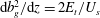
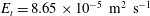
 $$\begin{eqnarray}\frac{\text{d}b_{g}^{2}}{\text{d}z}=\unicode[STIX]{x1D6FD}_{t}=2E_{t}U_{s}^{-1}\quad \Rightarrow \quad b_{g}=\sqrt{2}E_{t}^{1/2}z^{1/2}U_{s}^{-1/2}.\end{eqnarray}$$
The measured plume width can be used with this equation to estimate $E_{t}$
. We perform a regression to the measured data on the width of the plumes, which follow a linear spreading process with
$E_{t}$
. We perform a regression to the measured data on the width of the plumes, which follow a linear spreading process with $b_{g}=0.1z$
for
$b_{g}=0.1z$
for $z/D<5$
from a point source, followed by a diffusive process with
$z/D<5$
from a point source, followed by a diffusive process with $\text{d}b_{g}^{2}/\text{d}z=2E_{t}/U_{s}$
for
$\text{d}b_{g}^{2}/\text{d}z=2E_{t}/U_{s}$
for $z/D\geqslant 5$
. From the regression to the data for
$z/D\geqslant 5$
. From the regression to the data for $b_{g}$
, we obtain
$b_{g}$
, we obtain $E_{t}=8.65\times 10^{-5}~\text{m}^{2}~\text{s}^{-1}$
for
$E_{t}=8.65\times 10^{-5}~\text{m}^{2}~\text{s}^{-1}$
for $Q_{1}$
and
$Q_{1}$
and $1.07\times 10^{-4}~\text{m}^{2}~\text{s}^{-1}$
for
$1.07\times 10^{-4}~\text{m}^{2}~\text{s}^{-1}$
for $Q_{2}$
; for fitting to data for
$Q_{2}$
; for fitting to data for $b_{\unicode[STIX]{x1D712}}$
, we obtain
$b_{\unicode[STIX]{x1D712}}$
, we obtain $E_{t}=3.98\times 10^{-5}~\text{m}^{2}~\text{s}^{-1}$
at the lower gas flow rate and
$E_{t}=3.98\times 10^{-5}~\text{m}^{2}~\text{s}^{-1}$
at the lower gas flow rate and $5.02\times 10^{-5}~\text{m}^{2}~\text{s}^{-1}$
at the higher release rate (see also table 2).
$5.02\times 10^{-5}~\text{m}^{2}~\text{s}^{-1}$
at the higher release rate (see also table 2).
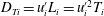
Table 2. Effective lateral diffusion coefficient from the data fit and estimated from two different mechanisms. For $D_{T}$
and
$D_{T}$
and $D_{E}$
, mean
$D_{E}$
, mean $\pm$
standard deviation calculated from data for all heights are shown.
$\pm$
standard deviation calculated from data for all heights are shown.

The differences in $E_{t}$
estimated from
$E_{t}$
estimated from $b_{g}$
and
$b_{g}$
and $b_{\unicode[STIX]{x1D712}}$
relate to the different spreading rates for velocity and concentration. This effect is normally quantified by the spreading ratio
$b_{\unicode[STIX]{x1D712}}$
relate to the different spreading rates for velocity and concentration. This effect is normally quantified by the spreading ratio $\unicode[STIX]{x1D706}_{b}$
, given by
$\unicode[STIX]{x1D706}_{b}$
, given by
 $$\begin{eqnarray}\unicode[STIX]{x1D706}_{b}=\frac{b_{\unicode[STIX]{x1D712}}}{b_{g}}.\end{eqnarray}$$
Here, we can estimate $\unicode[STIX]{x1D706}_{b}$
by
$\unicode[STIX]{x1D706}_{b}$
by $\sqrt{E_{\unicode[STIX]{x1D712}}/E_{g}}$
, as well as from the direct calculation from the definition; the values for our data are reported in table 2. These values can be compared to those reported by Socolofsky & Adams (Reference Socolofsky and Adams2005), who computed
$\sqrt{E_{\unicode[STIX]{x1D712}}/E_{g}}$
, as well as from the direct calculation from the definition; the values for our data are reported in table 2. These values can be compared to those reported by Socolofsky & Adams (Reference Socolofsky and Adams2005), who computed $\unicode[STIX]{x1D706}_{b}$
between
$\unicode[STIX]{x1D706}_{b}$
between $b_{\unicode[STIX]{x1D712}}$
and
$b_{\unicode[STIX]{x1D712}}$
and $b_{c}$
, the half-width of the concentration distribution. If we use the single-phase relationship
$b_{c}$
, the half-width of the concentration distribution. If we use the single-phase relationship $b_{c}=1.2b_{g}$
, our values of
$b_{c}=1.2b_{g}$
, our values of $\unicode[STIX]{x1D706}_{b}$
reported here are similar to those in Socolofsky & Adams (Reference Socolofsky and Adams2005) for bubble plumes with very weak entrained fluid velocity. Hence, the differences in the observed values of
$\unicode[STIX]{x1D706}_{b}$
reported here are similar to those in Socolofsky & Adams (Reference Socolofsky and Adams2005) for bubble plumes with very weak entrained fluid velocity. Hence, the differences in the observed values of $E_{t}$
for fitting to
$E_{t}$
for fitting to $b_{g}$
and
$b_{g}$
and $b_{\unicode[STIX]{x1D712}}$
also match expectations for weak bubble plumes.
$b_{\unicode[STIX]{x1D712}}$
also match expectations for weak bubble plumes.
The turbulent dispersion in natural or engineered water systems can be described by an analogy to Fickian or molecular diffusion, and the diffusion coefficient is termed ‘turbulent diffusivity’ in turbulent flows. Since the ambient water is stagnant in the current experiment, the turbulent diffusion coefficient in the background is likely to be very low. Therefore, the diffusive process of the bubble spreading may be the result of two mechanisms: (1) the turbulent wake flow behind the leading bubbles; and (2) the lateral excursion of the bubbles, considering the zigzag or helical paths of these ellipsoidal wobbling bubbles (Wang et al. Reference Wang, Socolofsky, Breier and Seewald2016).
Here, we estimate the effective lateral diffusion coefficient for each of the above mechanisms. First, we estimate the turbulent diffusivity ( $D_{T}$
) in the wake flow in three directions (i.e. bubble rising direction
$D_{T}$
) in the wake flow in three directions (i.e. bubble rising direction $z$
, seeding flow direction
$z$
, seeding flow direction $x$
, and binormal direction
$x$
, and binormal direction $y$
). We applied an approach derived from Taylor’s theory following Holtappels & Lorke (Reference Holtappels and Lorke2011), giving turbulent diffusivity
$y$
). We applied an approach derived from Taylor’s theory following Holtappels & Lorke (Reference Holtappels and Lorke2011), giving turbulent diffusivity $D_{Ti}=u_{i}^{\prime }L_{i}=u_{i}^{\prime 2}T_{i}$
, where
$D_{Ti}=u_{i}^{\prime }L_{i}=u_{i}^{\prime 2}T_{i}$
, where $u^{\prime }$
is the turbulent velocity scale,
$u^{\prime }$
is the turbulent velocity scale, $L$
is the integral length scale,
$L$
is the integral length scale, $T$
is the integral time scale and
$T$
is the integral time scale and $i$
indicates the direction. In this work,
$i$
indicates the direction. In this work, $u_{i}^{\prime }$
is the standard deviation of the velocity measured by the ADV and
$u_{i}^{\prime }$
is the standard deviation of the velocity measured by the ADV and $T_{i}$
is calculated by taking the integral of the autocorrelation function of the ADV data on the centreline (Tennekes & Lumley Reference Tennekes and Lumley1972; Holtappels & Lorke Reference Holtappels and Lorke2011). The estimated turbulent diffusivity is shown in figure 7. It is seen that
$T_{i}$
is calculated by taking the integral of the autocorrelation function of the ADV data on the centreline (Tennekes & Lumley Reference Tennekes and Lumley1972; Holtappels & Lorke Reference Holtappels and Lorke2011). The estimated turbulent diffusivity is shown in figure 7. It is seen that $D_{T}$
for
$D_{T}$
for $Q_{2}$
is higher than that for
$Q_{2}$
is higher than that for $Q_{1}$
in all three directions, and
$Q_{1}$
in all three directions, and $D_{T,z}$
is slightly larger than those in the other two directions. Overall, on the horizontal directions,
$D_{T,z}$
is slightly larger than those in the other two directions. Overall, on the horizontal directions, $D_{T}$
is in the range of
$D_{T}$
is in the range of $10^{-6}~\text{m}^{2}~\text{s}^{-1}$
, and is approximately an order of magnitude smaller than
$10^{-6}~\text{m}^{2}~\text{s}^{-1}$
, and is approximately an order of magnitude smaller than $E_{t}$
estimated from the plume spreading data.
$E_{t}$
estimated from the plume spreading data.

Figure 7. Turbulent diffusivity at different heights for $Q_{1}$
and
$Q_{1}$
and $Q_{2}$
, estimated using Taylor’s theory (Holtappels & Lorke Reference Holtappels and Lorke2011). Symbols present the data in the bubble plumes; the solid and dashed black lines represent the mean value and standard deviation of the diffusivity in a test run without the bubble plume but with the seeding flow.
$Q_{2}$
, estimated using Taylor’s theory (Holtappels & Lorke Reference Holtappels and Lorke2011). Symbols present the data in the bubble plumes; the solid and dashed black lines represent the mean value and standard deviation of the diffusivity in a test run without the bubble plume but with the seeding flow.
The effective diffusion coefficient due to the second mechanism of bubble wobbling can be estimated from the product of the distance and velocity scales of the lateral excursion of the bubble motion:
 $$\begin{eqnarray}D_{E}=L_{E}U_{E},\end{eqnarray}$$
where $L_{E}$
is the mean of bubble lateral excursion distance and
$L_{E}$
is the mean of bubble lateral excursion distance and $U_{E}$
is the mean lateral velocity of the bubble excursion. The three-dimensional measurements of bubble location from the stereo camera data provide the information to compute these scales, and the calculated effective diffusion coefficients are reported in table 2. The
$U_{E}$
is the mean lateral velocity of the bubble excursion. The three-dimensional measurements of bubble location from the stereo camera data provide the information to compute these scales, and the calculated effective diffusion coefficients are reported in table 2. The $E_{t}$
calculated by fitting the void fraction is closer to
$E_{t}$
calculated by fitting the void fraction is closer to $D_{E}$
than
$D_{E}$
than $D_{T}$
. In addition, the similar
$D_{T}$
. In addition, the similar $E_{t}$
for both gas flow rates shown in the data may be well explained by the bubble excursion, which is determined by the bubble sizes, and is independent of the initial gas flow rate at these low flow rates. Here, we conclude that the bubble lateral excursion is probably a major contributing mechanism that is responsible for the spreading of the weak bubble plume in stagnant water, and the effective diffusion coefficient is determined by the extent and velocity of the lateral bubble motion. In more turbulent water systems, the turbulent diffusion may have a more profound contribution to the bubble plume spreading, but this is subject to further studies beyond our present scope. In any case, by these analyses, we conclude that a weak bubble plume spreads out by a diffusion process acting on the dispersed-phase particles.
$E_{t}$
for both gas flow rates shown in the data may be well explained by the bubble excursion, which is determined by the bubble sizes, and is independent of the initial gas flow rate at these low flow rates. Here, we conclude that the bubble lateral excursion is probably a major contributing mechanism that is responsible for the spreading of the weak bubble plume in stagnant water, and the effective diffusion coefficient is determined by the extent and velocity of the lateral bubble motion. In more turbulent water systems, the turbulent diffusion may have a more profound contribution to the bubble plume spreading, but this is subject to further studies beyond our present scope. In any case, by these analyses, we conclude that a weak bubble plume spreads out by a diffusion process acting on the dispersed-phase particles.
4.2 Plume centreline velocity
The evolution of the centreline velocity with distance along the plume axis in a classic single-phase plume has been well documented. Fisher et al. (Reference Fisher, List, Koh, Imberger and Brooks1979) show that the centreline velocity scales with $z^{-1/3}$
in a continuous-phase plume. For classic bubble plumes, Bombardelli et al. (Reference Bombardelli, Buscaglia, Rehmann, Rincon and Garcia2007) showed that
$z^{-1/3}$
in a continuous-phase plume. For classic bubble plumes, Bombardelli et al. (Reference Bombardelli, Buscaglia, Rehmann, Rincon and Garcia2007) showed that
 $$\begin{eqnarray}\frac{U_{m}}{U_{s}}\sim \left(\frac{z}{D}\right)^{-1/3},\end{eqnarray}$$
for an integral bubble plume model for $z/D<5$
. This scaling is usually assumed to be valid in a classic bubble plume (Lemckert & Imberger Reference Lemckert and Imberger1993). The data of Fannelop & Sjoen (Reference Fannelop and Sjoen1980), Milgram & Van Houten (Reference Milgram and Van Houten1982) and Milgram (Reference Milgram1983) are close to this scaling, although they do not collapse onto it (see figure 6a in Bombardelli et al. (Reference Bombardelli, Buscaglia, Rehmann, Rincon and Garcia2007) and figure 8 in the present paper).
$z/D<5$
. This scaling is usually assumed to be valid in a classic bubble plume (Lemckert & Imberger Reference Lemckert and Imberger1993). The data of Fannelop & Sjoen (Reference Fannelop and Sjoen1980), Milgram & Van Houten (Reference Milgram and Van Houten1982) and Milgram (Reference Milgram1983) are close to this scaling, although they do not collapse onto it (see figure 6a in Bombardelli et al. (Reference Bombardelli, Buscaglia, Rehmann, Rincon and Garcia2007) and figure 8 in the present paper).

Figure 8. Normalized centreline water velocity $U_{m}$
(with respect to the bubble slip velocity,
$U_{m}$
(with respect to the bubble slip velocity, $U_{s}$
) versus height
$U_{s}$
) versus height $z$
above the orifice (with respect to the length scale
$z$
above the orifice (with respect to the length scale $D$
), where
$D$
), where $D$
is the length scale defined in Bombardelli et al. (Reference Bombardelli, Buscaglia, Rehmann, Rincon and Garcia2007). The
$D$
is the length scale defined in Bombardelli et al. (Reference Bombardelli, Buscaglia, Rehmann, Rincon and Garcia2007). The $Q_{1}$
and
$Q_{1}$
and $Q_{2}$
in the legend are the data of the present study. Milgram83, MV82 and FS80 represent the data summarized in Milgram (Reference Milgram1983), including those from Fannelop & Sjoen (Reference Fannelop and Sjoen1980) (shown as FS80) and Milgram & Van Houten (Reference Milgram and Van Houten1982) (shown as MV82). The dashed lines show the slopes of
$Q_{2}$
in the legend are the data of the present study. Milgram83, MV82 and FS80 represent the data summarized in Milgram (Reference Milgram1983), including those from Fannelop & Sjoen (Reference Fannelop and Sjoen1980) (shown as FS80) and Milgram & Van Houten (Reference Milgram and Van Houten1982) (shown as MV82). The dashed lines show the slopes of $-1/3$
and
$-1/3$
and $-1/2$
for classic and weak plumes, respectively.
$-1/2$
for classic and weak plumes, respectively.
Bombardelli et al. (Reference Bombardelli, Buscaglia, Rehmann, Rincon and Garcia2007) obtained an analytical solution for the centreline velocity for $z/D\gg 1$
in a classical integral bubble plume model, namely
$z/D\gg 1$
in a classical integral bubble plume model, namely
 $$\begin{eqnarray}\frac{U_{m}}{U_{s}}=3\left(\frac{z}{D}\right)^{-1/2},\quad \text{for}~z/D\gg 1.\end{eqnarray}$$
Bombardelli et al. (Reference Bombardelli, Buscaglia, Rehmann, Rincon and Garcia2007) also used numerous simulation results to obtain the asymptotic equation:
 $$\begin{eqnarray}\frac{U_{m}}{U_{s}}=2\left(\frac{1.9(z/D)^{-1}}{1+0.563(z/D)^{1/2}}\right)^{1/3},\quad \text{for}~z/D>5.\end{eqnarray}$$
Figure 8 shows that the non-dimensional relationship between the centreline velocity in the plume and the height above the orifice for our data ( $z/D>5$
) and the literature data (
$z/D>5$
) and the literature data ( $z/D<5$
) falls in the vicinity of the prediction line given by (4.7). Our data and the data from the literature span the value of
$z/D<5$
) falls in the vicinity of the prediction line given by (4.7). Our data and the data from the literature span the value of $z/D$
over four orders of magnitude. Although the discrepancy from the prediction line (4.7) grows for
$z/D$
over four orders of magnitude. Although the discrepancy from the prediction line (4.7) grows for $z/D<0.5$
, it does pass through our weak bubble plume data and matches the observations over nearly the entire range of
$z/D<0.5$
, it does pass through our weak bubble plume data and matches the observations over nearly the entire range of $z/D$
. Thus, we will consider (4.7) valid for classic and weak bubble plumes.
$z/D$
. Thus, we will consider (4.7) valid for classic and weak bubble plumes.
This result also seems to suggest that a classic integral model can quantitatively predict the centreline velocity in both classic and weak bubble plumes. However, this asymptotic solution is solved on the basis of a linear spreading hypothesis or constant entrainment coefficient hypothesis (see also later discussion in § 4.4). As a result, it cannot predict the correct plume spreading for the weak bubble plume (see figure 6
a), because the integral model with constant $\unicode[STIX]{x1D6FC}$
will follow
$\unicode[STIX]{x1D6FC}$
will follow $b_{g}=\unicode[STIX]{x1D6FD}z$
. Hence, the classic integral theory for a bubble plume is incapable of predicting the correct evolution of the liquid volume flux
$b_{g}=\unicode[STIX]{x1D6FD}z$
. Hence, the classic integral theory for a bubble plume is incapable of predicting the correct evolution of the liquid volume flux $Q=\unicode[STIX]{x03C0}b_{g}^{2}U_{m}$
in weak bubble plumes (
$Q=\unicode[STIX]{x03C0}b_{g}^{2}U_{m}$
in weak bubble plumes ( $z/D>5$
) since it will estimate a correct
$z/D>5$
) since it will estimate a correct $U_{m}$
while significantly overestimating
$U_{m}$
while significantly overestimating $b_{g}$
.
$b_{g}$
.
4.3 Liquid volume flux
In a general case, the relationship between $Q$
and
$Q$
and $z$
in a plume is expected to follow a power law
$z$
in a plume is expected to follow a power law $Q\sim z^{m}$
(Leitch & Baines Reference Leitch and Baines1989). Because
$Q\sim z^{m}$
(Leitch & Baines Reference Leitch and Baines1989). Because $\text{d}Q/\text{d}z\sim z^{m-1}$
represents the increase of liquid volume flux over height, which is due to the entrainment of ambient water, the value of
$\text{d}Q/\text{d}z\sim z^{m-1}$
represents the increase of liquid volume flux over height, which is due to the entrainment of ambient water, the value of $m$
can be understood as follows:
$m$
can be understood as follows:
(i) $m>1$
,
$Q$
increases faster than linearly (i.e. increasing entrainment);
$m>1$
,
$Q$
increases faster than linearly (i.e. increasing entrainment);(ii)
$m=1$
,
$Q$
increases linearly (i.e. constant entrainment);(iii)
$m<1$
,
$Q$
increases slower than linearly (i.e. decreasing entrainment);(iv)
$m=0$
,
$Q$
does not change (i.e. no entrainment); and(v)
$m<0$
,
$Q$
decreases (i.e. detrainment).


From (4.5) and (3.2), the liquid volume flux in a classic integral model of a bubble plume can be derived as
 $$\begin{eqnarray}Q=\unicode[STIX]{x03C0}b_{g}^{2}U_{m}\sim \unicode[STIX]{x03C0}\unicode[STIX]{x1D6FD}^{2}U_{s}D^{1/3}z^{5/3}.\end{eqnarray}$$
Equation (4.8) suggests that in a classic plume $Q$
increases faster than linearly as
$Q$
increases faster than linearly as $m=5/3$
. Most of the literature data for bubble plumes (Fannelop & Sjoen Reference Fannelop and Sjoen1980; Milgram & Van Houten Reference Milgram and Van Houten1982; Milgram Reference Milgram1983) have
$m=5/3$
. Most of the literature data for bubble plumes (Fannelop & Sjoen Reference Fannelop and Sjoen1980; Milgram & Van Houten Reference Milgram and Van Houten1982; Milgram Reference Milgram1983) have $m$
values slightly smaller than
$m$
values slightly smaller than $5/3$
, with the majority of these data observed in the classic bubble plume regime, below the asymptotic region (i.e.
$5/3$
, with the majority of these data observed in the classic bubble plume regime, below the asymptotic region (i.e. $z/D<5$
). This is a result of the presence of
$z/D<5$
). This is a result of the presence of $D$
, which violates the requirements for self-similarity, and expresses itself through a non-constant entrainment coefficient (or spreading rate
$D$
, which violates the requirements for self-similarity, and expresses itself through a non-constant entrainment coefficient (or spreading rate $\unicode[STIX]{x1D6FD}$
). Milgram (Reference Milgram1983) developed a detailed theory for the entrainment coefficient in classic bubble plumes (see § 4.4), but most of the variability is near the source, and many successful models employ constant entrainment coefficients (Asaeda & Imberger Reference Asaeda and Imberger1993; Bombardelli et al.
Reference Bombardelli, Buscaglia, Rehmann, Rincon and Garcia2007; Socolofsky, Bhaumik & Seol Reference Socolofsky, Bhaumik and Seol2008).
$\unicode[STIX]{x1D6FD}$
). Milgram (Reference Milgram1983) developed a detailed theory for the entrainment coefficient in classic bubble plumes (see § 4.4), but most of the variability is near the source, and many successful models employ constant entrainment coefficients (Asaeda & Imberger Reference Asaeda and Imberger1993; Bombardelli et al.
Reference Bombardelli, Buscaglia, Rehmann, Rincon and Garcia2007; Socolofsky, Bhaumik & Seol Reference Socolofsky, Bhaumik and Seol2008).
Using the operational definition $Q=\unicode[STIX]{x03C0}b_{g}^{2}U_{m}$
, we can derive an equivalent expression in the weak bubble plume regime from our data. We select the diffusion growth process for plume spreading and substitute (4.2) for
$Q=\unicode[STIX]{x03C0}b_{g}^{2}U_{m}$
, we can derive an equivalent expression in the weak bubble plume regime from our data. We select the diffusion growth process for plume spreading and substitute (4.2) for $b_{g}$
. For the centreline velocity, we use the asymptotic solution at large
$b_{g}$
. For the centreline velocity, we use the asymptotic solution at large $z/D\gg 1$
(4.6). This yields
$z/D\gg 1$
(4.6). This yields
 $$\begin{eqnarray}Q=6\unicode[STIX]{x03C0}E_{t}z^{1/2}D^{1/2}.\end{eqnarray}$$
From these fitted equations, $Q$
scales with
$Q$
scales with $z^{1/2}$
in the weak plume, which demonstrates a decreasing entrainment of ambient water (i.e.
$z^{1/2}$
in the weak plume, which demonstrates a decreasing entrainment of ambient water (i.e. $m<1$
). Therefore, the weak and classic bubble plumes have different entrainment processes (increasing and decreasing) and follow different scaling laws (
$m<1$
). Therefore, the weak and classic bubble plumes have different entrainment processes (increasing and decreasing) and follow different scaling laws ( $m=1/2$
and
$m=1/2$
and $m=5/3$
). In the intermediate range of
$m=5/3$
). In the intermediate range of $z/D\sim O(1)$
,
$z/D\sim O(1)$
, $m$
is expected to be in the range between
$m$
is expected to be in the range between $1/2$
and
$1/2$
and $5/3$
.
$5/3$
.
Here, we also consider the similar laboratory measurements in weak bubble plumes by Leitch & Baines (Reference Leitch and Baines1989). They observed the same bubble spreading rate ( $b_{g}\sim z^{1/2}$
) but report a different
$b_{g}\sim z^{1/2}$
) but report a different $m$
(
$m$
( $m=1$
in their work instead of
$m=1$
in their work instead of $m=1/2$
in this study). This discrepancy follows from their observation of
$m=1/2$
in this study). This discrepancy follows from their observation of $U_{m}(z)\sim z^{0}$
instead of
$U_{m}(z)\sim z^{0}$
instead of $U_{m}(z)\sim z^{-1/2}$
. Their observation may represent an accurate measurement, which the scatter in figure 8 allows, or may result from their shallow experimental water depth (i.e. 0.5 m), which may not allow adequate development of the velocity gradient to observe the
$U_{m}(z)\sim z^{-1/2}$
. Their observation may represent an accurate measurement, which the scatter in figure 8 allows, or may result from their shallow experimental water depth (i.e. 0.5 m), which may not allow adequate development of the velocity gradient to observe the $-1/2$
power law. In our experiments, the observations were conducted over 16 m of water depth, and the
$-1/2$
power law. In our experiments, the observations were conducted over 16 m of water depth, and the $-1/2$
power law is consistent across this whole water depth, linking our experiments to results reported in Milgram & Van Houten (Reference Milgram and Van Houten1982). Hence, we conclude that
$-1/2$
power law is consistent across this whole water depth, linking our experiments to results reported in Milgram & Van Houten (Reference Milgram and Van Houten1982). Hence, we conclude that $m=1/2$
is the more accurate estimate of the entrainment process in a weak bubble plume.
$m=1/2$
is the more accurate estimate of the entrainment process in a weak bubble plume.
4.4 Apparent entrainment coefficient
In single-phase jets and plumes, an integral model is usually closed using an entrainment hypothesis or a spreading hypothesis, and the two hypotheses are equivalent (Lee & Chu Reference Lee and Chu2003) (see also appendix A). A similar spreading hypothesis was recently adapted to a particle plume (Lai et al. Reference Lai, Chan, Law and Adams2016). The equivalence of these two hypotheses can be summarized as follows:
 $$\begin{eqnarray}entrainment~hypothesis~(for~Gaussian~profile)\quad \frac{\text{d}Q}{\text{d}z}=2\unicode[STIX]{x03C0}b_{g}\unicode[STIX]{x1D6FC}U_{m},\end{eqnarray}$$
is equivalent to
 $$\begin{eqnarray}\displaystyle & \displaystyle jet\left\{\begin{array}{@{}ll@{}}linear~spreading\quad & \unicode[STIX]{x1D6FD}_{j}={\displaystyle \frac{\text{d}b_{g}}{\text{d}z}},\\ dimensional~analysis\quad & U_{m}=\left({\displaystyle \frac{M_{0}}{z^{2}}}\right)^{1/2},\end{array}\right. & \displaystyle\end{eqnarray}$$
 $$\begin{eqnarray}\displaystyle & \displaystyle plume\left\{\begin{array}{@{}ll@{}}linear~spreading\quad & \unicode[STIX]{x1D6FD}_{p}={\displaystyle \frac{\text{d}b_{g}}{\text{d}z}},\\ dimensional~analysis\quad & U_{m}=\left({\displaystyle \frac{B_{0}}{z}}\right)^{1/3},\end{array}\right. & \displaystyle\end{eqnarray}$$
where $M_{0}$
is the initial kinematic momentum flux of the jet. Thus, linear spreading of the single-phase jet and plume is mathematically equivalent to the entrainment hypothesis with a constant entrainment coefficient
$M_{0}$
is the initial kinematic momentum flux of the jet. Thus, linear spreading of the single-phase jet and plume is mathematically equivalent to the entrainment hypothesis with a constant entrainment coefficient $\unicode[STIX]{x1D6FC}$
. The entrainment hypothesis states that the growth of the liquid volume flux is due to the shear entrainment of ambient liquid at the edge of the jet or plume with the entrainment velocity
$\unicode[STIX]{x1D6FC}$
. The entrainment hypothesis states that the growth of the liquid volume flux is due to the shear entrainment of ambient liquid at the edge of the jet or plume with the entrainment velocity $U_{e}$
, where
$U_{e}$
, where $U_{e}$
is proportional to the centreline velocity multiplied by the entrainment coefficient
$U_{e}$
is proportional to the centreline velocity multiplied by the entrainment coefficient $\unicode[STIX]{x1D6FC}$
(Turner Reference Turner1986). Because the classic bubble plume spreads out linearly, similar to single-phase jets and plumes, the entrainment hypothesis in single-phase jets and plumes is adopted for many integral models of the classic bubble plume (Asaeda & Imberger Reference Asaeda and Imberger1993; Bombardelli et al.
Reference Bombardelli, Buscaglia, Rehmann, Rincon and Garcia2007; Socolofsky et al.
Reference Socolofsky, Bhaumik and Seol2008; Dissanayake, Gros & Socolofsky Reference Dissanayake, Gros and Socolofsky2018).
$\unicode[STIX]{x1D6FC}$
(Turner Reference Turner1986). Because the classic bubble plume spreads out linearly, similar to single-phase jets and plumes, the entrainment hypothesis in single-phase jets and plumes is adopted for many integral models of the classic bubble plume (Asaeda & Imberger Reference Asaeda and Imberger1993; Bombardelli et al.
Reference Bombardelli, Buscaglia, Rehmann, Rincon and Garcia2007; Socolofsky et al.
Reference Socolofsky, Bhaumik and Seol2008; Dissanayake, Gros & Socolofsky Reference Dissanayake, Gros and Socolofsky2018).
For the weak bubble plume, a formulation of the integral plume equations with a constant entrainment breaks down. Instead, we derive the gradient of liquid volume flux from a spreading hypothesis, following the same procedure as in single-phase flow (see appendix A) to obtain
 $$\begin{eqnarray}\frac{\text{d}Q}{\text{d}z}=\frac{1}{2}\unicode[STIX]{x03C0}\unicode[STIX]{x1D6FD}_{b}U_{m},\end{eqnarray}$$
with $\unicode[STIX]{x1D6FD}_{b}=\text{d}b_{g}^{2}/\text{d}z$
. This equation differs fundamentally from the constant entrainment hypothesis (i.e. equation (4.10)). The form of (4.13) also suggests that the characteristic length scale where entrainment occurs is not
$\unicode[STIX]{x1D6FD}_{b}=\text{d}b_{g}^{2}/\text{d}z$
. This equation differs fundamentally from the constant entrainment hypothesis (i.e. equation (4.10)). The form of (4.13) also suggests that the characteristic length scale where entrainment occurs is not $b_{g}$
. We suspect that there is no entrainment at the edge of the weak bubble plume, giving
$b_{g}$
. We suspect that there is no entrainment at the edge of the weak bubble plume, giving $U_{e}=0$
. Instead, the growth of the liquid volume flux in the weak bubble plume is due to the increasing width of the plume as the result of diffusive spreading of the bubbles and the changing wake flow below the leading bubbles as they spread out. This hypothesis is also consistent with ideas in Leitch & Baines (Reference Leitch and Baines1989), who attributed the flow rate in a weak bubble plume to the individual wakes behind bubbles.
$U_{e}=0$
. Instead, the growth of the liquid volume flux in the weak bubble plume is due to the increasing width of the plume as the result of diffusive spreading of the bubbles and the changing wake flow below the leading bubbles as they spread out. This hypothesis is also consistent with ideas in Leitch & Baines (Reference Leitch and Baines1989), who attributed the flow rate in a weak bubble plume to the individual wakes behind bubbles.
Although we conclude for a weak bubble plume that there is no entrainment velocity in the normal sense of a plume, the equation for the growth rate of the liquid volume flux can be treated mathematically in the same manner as a classic plume, but with a different interpretation of the entrainment coefficient. If we combine (4.10) and (4.13), we can obtain the relationship
 $$\begin{eqnarray}\unicode[STIX]{x1D6FC}=\frac{\unicode[STIX]{x1D6FD}_{b}}{4b_{g}}.\end{eqnarray}$$
Here, we name $\unicode[STIX]{x1D6FC}$
the ‘apparent entrainment coefficient’, as it represents the mathematical formulation of entrainment, but in a system that does not obey the entrainment hypothesis. This equation predicts that
$\unicode[STIX]{x1D6FC}$
the ‘apparent entrainment coefficient’, as it represents the mathematical formulation of entrainment, but in a system that does not obey the entrainment hypothesis. This equation predicts that $\unicode[STIX]{x1D6FC}$
is not a constant and is proportional to the turbulent diffusivity causing the spread of the bubbles (
$\unicode[STIX]{x1D6FC}$
is not a constant and is proportional to the turbulent diffusivity causing the spread of the bubbles ( $\unicode[STIX]{x1D6FD}_{b}$
) and inversely proportional to the width of the plume (
$\unicode[STIX]{x1D6FD}_{b}$
) and inversely proportional to the width of the plume ( $b_{g}(z)$
). Using the definitions of
$b_{g}(z)$
). Using the definitions of $\unicode[STIX]{x1D6FD}_{b}$
and
$\unicode[STIX]{x1D6FD}_{b}$
and $b_{g}(z)$
in (4.2), we obtain
$b_{g}(z)$
in (4.2), we obtain
 $$\begin{eqnarray}\unicode[STIX]{x1D6FC}=2^{-3/2}E_{t}^{1/2}U_{s}^{-1/2}z^{-1/2},\end{eqnarray}$$
and (4.13) becomes (this is also the direct derivative of (4.9))
 $$\begin{eqnarray}\frac{\text{d}Q}{\text{d}z}=3\unicode[STIX]{x03C0}E_{t}z^{-1/2}D^{1/2}.\end{eqnarray}$$
Equation (4.15) predicts that the apparent entrainment coefficient $\unicode[STIX]{x1D6FC}$
decreases with height following
$\unicode[STIX]{x1D6FC}$
decreases with height following $\unicode[STIX]{x1D6FC}\sim z^{-1/2}$
in the weak bubble plume. In a single-phase round jet or plume, the constant Gaussian entrainment coefficients are
$\unicode[STIX]{x1D6FC}\sim z^{-1/2}$
in the weak bubble plume. In a single-phase round jet or plume, the constant Gaussian entrainment coefficients are $\unicode[STIX]{x1D6FC}=0.057$
and 0.083, respectively (Lee & Chu Reference Lee and Chu2003). Although integral models for classic bubble plumes also usually assume constant entrainment, many experimentalists have found that
$\unicode[STIX]{x1D6FC}=0.057$
and 0.083, respectively (Lee & Chu Reference Lee and Chu2003). Although integral models for classic bubble plumes also usually assume constant entrainment, many experimentalists have found that $\unicode[STIX]{x1D6FC}$
is not a constant in bubble plumes, and this arises because the classic bubble plume is not strictly self-similar. Milgram (Reference Milgram1983) used a saturation growth curve to describe the relationship between the entrainment coefficient and a local bubble Froude number (defined by
$\unicode[STIX]{x1D6FC}$
is not a constant in bubble plumes, and this arises because the classic bubble plume is not strictly self-similar. Milgram (Reference Milgram1983) used a saturation growth curve to describe the relationship between the entrainment coefficient and a local bubble Froude number (defined by $F_{B}=Q_{b}^{2/5}\unicode[STIX]{x1D712}^{1/3}g^{3/10}\unicode[STIX]{x0394}\unicode[STIX]{x1D70C}^{1/2}\unicode[STIX]{x1D70E}^{-1/2}$
, where
$F_{B}=Q_{b}^{2/5}\unicode[STIX]{x1D712}^{1/3}g^{3/10}\unicode[STIX]{x0394}\unicode[STIX]{x1D70C}^{1/2}\unicode[STIX]{x1D70E}^{-1/2}$
, where $Q_{b}$
is gas volume flux). In his empirical fit to data, the entrainment coefficient approaches a plateau at 0.16 when the local bubble Froude number increases, which occurs close to the release (e.g.
$Q_{b}$
is gas volume flux). In his empirical fit to data, the entrainment coefficient approaches a plateau at 0.16 when the local bubble Froude number increases, which occurs close to the release (e.g. $z/D\rightarrow 0$
). Figure 9 compares our data with this empirical curve, where we computed the apparent entrainment coefficient
$z/D\rightarrow 0$
). Figure 9 compares our data with this empirical curve, where we computed the apparent entrainment coefficient $\unicode[STIX]{x1D6FC}$
at mid-points between measurements using (4.10). The apparent entrainment coefficients in our experiment are approximately an order of magnitude smaller than entrainment coefficients reported by previous authors for larger
$\unicode[STIX]{x1D6FC}$
at mid-points between measurements using (4.10). The apparent entrainment coefficients in our experiment are approximately an order of magnitude smaller than entrainment coefficients reported by previous authors for larger $z/D$
and show remarkable correspondence with the empirical fit of Milgram (Reference Milgram1983).
$z/D$
and show remarkable correspondence with the empirical fit of Milgram (Reference Milgram1983).

Figure 9. The relationship between $\unicode[STIX]{x1D6FC}$
and local bubble Froude number, defined after Milgram (Reference Milgram1983), where
$\unicode[STIX]{x1D6FC}$
and local bubble Froude number, defined after Milgram (Reference Milgram1983), where $\unicode[STIX]{x1D6FC}$
is the entrainment coefficient in the classic bubble plume and is the apparent entrainment coefficient in the weak bubble plume. The dashed line represents the saturation curve proposed by Milgram (Reference Milgram1983).
$\unicode[STIX]{x1D6FC}$
is the entrainment coefficient in the classic bubble plume and is the apparent entrainment coefficient in the weak bubble plume. The dashed line represents the saturation curve proposed by Milgram (Reference Milgram1983).
Milgram (Reference Milgram1983) interpreted the local bubble Froude number $F_{B}$
as a ratio between the mixing length scale of turbulence in the plume and the characteristic length scale of bubble–bubble separation. The turbulence and the bubble–bubble separation change as the plume develops away from the source, and the resulting bubble Froude number is a complex nonlinear function of
$F_{B}$
as a ratio between the mixing length scale of turbulence in the plume and the characteristic length scale of bubble–bubble separation. The turbulence and the bubble–bubble separation change as the plume develops away from the source, and the resulting bubble Froude number is a complex nonlinear function of $z$
. However, this scaling law is hidden within the
$z$
. However, this scaling law is hidden within the $z$
dependence of the parameters that make up
$z$
dependence of the parameters that make up $F_{B}$
(e.g.
$F_{B}$
(e.g. $\unicode[STIX]{x1D712}$
,
$\unicode[STIX]{x1D712}$
, $Q_{b}$
and
$Q_{b}$
and $\unicode[STIX]{x0394}\unicode[STIX]{x1D70C}$
). Our analysis also predicts that
$\unicode[STIX]{x0394}\unicode[STIX]{x1D70C}$
). Our analysis also predicts that $\unicode[STIX]{x1D6FC}\sim z^{1/2}$
in a weak bubble plume. Hence, it is useful to evaluate the relationship between entrainment coefficient or apparent entrainment coefficient and the height above the source in the full range of the available bubble plume data. Figure 10 shows the relationship between
$\unicode[STIX]{x1D6FC}\sim z^{1/2}$
in a weak bubble plume. Hence, it is useful to evaluate the relationship between entrainment coefficient or apparent entrainment coefficient and the height above the source in the full range of the available bubble plume data. Figure 10 shows the relationship between $\unicode[STIX]{x1D6FC}$
and
$\unicode[STIX]{x1D6FC}$
and $z/D$
over a span of four orders of magnitude of
$z/D$
over a span of four orders of magnitude of $z/D$
, including both classic and weak bubble plumes. The constant entrainment coefficient in a continuous-phase plume, 0.083, and the plateau value in Milgram (Reference Milgram1983), 0.16, are shown for reference. A reference line of
$z/D$
, including both classic and weak bubble plumes. The constant entrainment coefficient in a continuous-phase plume, 0.083, and the plateau value in Milgram (Reference Milgram1983), 0.16, are shown for reference. A reference line of $\unicode[STIX]{x1D6FC}\sim z^{-1/2}$
is also shown, and our data agree well with this theoretical relationship in the region
$\unicode[STIX]{x1D6FC}\sim z^{-1/2}$
is also shown, and our data agree well with this theoretical relationship in the region $z/D>5$
.
$z/D>5$
.

Figure 10. The relationship between $\unicode[STIX]{x1D6FC}$
and the normalized height. The data key follows figure 8 with two additional datasets from Seol et al. (Reference Seol, Bhaumik, Bergmann and Socolofsky2007) (shown as SBBS07) and Hugi (Reference Hugi1993) (shown as Hugi93). Hugi’s data are directly digitized from the figure in Hugi (Reference Hugi1993) and are regrouped into two regimes: (1)
$\unicode[STIX]{x1D6FC}$
and the normalized height. The data key follows figure 8 with two additional datasets from Seol et al. (Reference Seol, Bhaumik, Bergmann and Socolofsky2007) (shown as SBBS07) and Hugi (Reference Hugi1993) (shown as Hugi93). Hugi’s data are directly digitized from the figure in Hugi (Reference Hugi1993) and are regrouped into two regimes: (1) $z/D$
in the same regime as our data, and (2)
$z/D$
in the same regime as our data, and (2) $z/D$
smaller than those of our data. The solid line is the reference of
$z/D$
smaller than those of our data. The solid line is the reference of $\unicode[STIX]{x1D6FC}\sim z^{-1/2}$
. The constant entrainment coefficient in a continuous-phase plume (i.e. 0.083) and the upper bound of a classic bubble plume (i.e. 0.16) suggested by Milgram (Reference Milgram1983) are plotted as dashed lines.
$\unicode[STIX]{x1D6FC}\sim z^{-1/2}$
. The constant entrainment coefficient in a continuous-phase plume (i.e. 0.083) and the upper bound of a classic bubble plume (i.e. 0.16) suggested by Milgram (Reference Milgram1983) are plotted as dashed lines.
These data have had different interpretations in past papers, each supported by part of the current complete dataset of observations. An asymptotic limit of entrainment coefficient is recognized in the classic bubble plume as $z\rightarrow 0$
but the value seems not to be universal. Ditmars & Cederwall (Reference Ditmars and Cederwall1974) suggested 0.082 (which does appear to be the correct bound as
$z\rightarrow 0$
but the value seems not to be universal. Ditmars & Cederwall (Reference Ditmars and Cederwall1974) suggested 0.082 (which does appear to be the correct bound as $D\rightarrow \infty$
, consistent with
$D\rightarrow \infty$
, consistent with $U_{s}\rightarrow 0$
) and Milgram (Reference Milgram1983) proposed 0.16 (which here appears as a peak near
$U_{s}\rightarrow 0$
) and Milgram (Reference Milgram1983) proposed 0.16 (which here appears as a peak near $z/D\sim O(0.1)$
). In addition, Seol et al. (Reference Seol, Bhaumik, Bergmann and Socolofsky2007) suggested a lower limit of entrainment coefficient (i.e. 0.04) for bubble plumes, a conclusion dominated by a single dataset of Hugi (Reference Hugi1993). Our data show significantly smaller
$z/D\sim O(0.1)$
). In addition, Seol et al. (Reference Seol, Bhaumik, Bergmann and Socolofsky2007) suggested a lower limit of entrainment coefficient (i.e. 0.04) for bubble plumes, a conclusion dominated by a single dataset of Hugi (Reference Hugi1993). Our data show significantly smaller $\unicode[STIX]{x1D6FC}$
compared to the cases with orders of magnitude smaller
$\unicode[STIX]{x1D6FC}$
compared to the cases with orders of magnitude smaller $z/D$
in the literature and invalidate the asymptotic assumption in Seol et al. (Reference Seol, Bhaumik, Bergmann and Socolofsky2007). Our
$z/D$
in the literature and invalidate the asymptotic assumption in Seol et al. (Reference Seol, Bhaumik, Bergmann and Socolofsky2007). Our $\unicode[STIX]{x1D6FC}$
values are also smaller than Hugi (Reference Hugi1993) (except for one data point), although both datasets are in a similar range of
$\unicode[STIX]{x1D6FC}$
values are also smaller than Hugi (Reference Hugi1993) (except for one data point), although both datasets are in a similar range of $z/D$
. The scattering of data for
$z/D$
. The scattering of data for $z/D>5$
might be due to the relatively large uncertainty associated with measuring
$z/D>5$
might be due to the relatively large uncertainty associated with measuring $\text{d}Q/\text{d}z$
from a finite difference approximation using an integral quantity, an error which should be less in our deep tank (16 m) compared to Hugi (3 m). Hence, despite the scatter, the bulk of the data seem to support a decreasing trend of
$\text{d}Q/\text{d}z$
from a finite difference approximation using an integral quantity, an error which should be less in our deep tank (16 m) compared to Hugi (3 m). Hence, despite the scatter, the bulk of the data seem to support a decreasing trend of $\unicode[STIX]{x1D6FC}$
versus
$\unicode[STIX]{x1D6FC}$
versus $z/D$
that is consistent with our scale relationship
$z/D$
that is consistent with our scale relationship $\unicode[STIX]{x1D6FC}\sim z^{-1/2}$
at large
$\unicode[STIX]{x1D6FC}\sim z^{-1/2}$
at large $z/D$
.
$z/D$
.
5 Unified scaling framework for classic and weak bubble plumes
From the above analysis, it is seen that the classic and weak bubble plumes are fundamentally different. In short, the weak bubble plume does not have classic shear entrainment, but rather spreads out by diffusion of the bubbles and has increasing plume volume flux due to changes in the wakes behind individual bubbles. A hypothetical, apparent entrainment coefficient for a weak bubble plume is a function of distance along the plume $z$
and is much smaller than for classic bubble plumes; this results in much lower spreading. Although the centreline velocity is within the prediction range of the relationship suggested by Bombardelli et al. (Reference Bombardelli, Buscaglia, Rehmann, Rincon and Garcia2007) (i.e. equation (4.7)), any model with a typical constant entrainment coefficient will overestimate the plume spreading, following the power law
$z$
and is much smaller than for classic bubble plumes; this results in much lower spreading. Although the centreline velocity is within the prediction range of the relationship suggested by Bombardelli et al. (Reference Bombardelli, Buscaglia, Rehmann, Rincon and Garcia2007) (i.e. equation (4.7)), any model with a typical constant entrainment coefficient will overestimate the plume spreading, following the power law $b_{g}\sim z$
instead of the correct diffusive spreading rate
$b_{g}\sim z$
instead of the correct diffusive spreading rate $b_{g}\sim z^{1/2}$
. If we simply decrease the constant entrainment coefficient in the model to match the correct apparent entrainment coefficient in the weak bubble plume, the model would fail to predict the velocity of the plume. Moreover, the linear spreading region governed by an approximately constant entrainment coefficient occurs in a narrow range of
$b_{g}\sim z^{1/2}$
. If we simply decrease the constant entrainment coefficient in the model to match the correct apparent entrainment coefficient in the weak bubble plume, the model would fail to predict the velocity of the plume. Moreover, the linear spreading region governed by an approximately constant entrainment coefficient occurs in a narrow range of $z/D<0.5$
. Hence, no integral model with a constant entrainment coefficient can accurately predict the liquid volume flux and plume width of a weak bubble plume for
$z/D<0.5$
. Hence, no integral model with a constant entrainment coefficient can accurately predict the liquid volume flux and plume width of a weak bubble plume for $z/D\gg 1$
, and it is necessary to include bubble diffusion in the plume spreading through the parameter
$z/D\gg 1$
, and it is necessary to include bubble diffusion in the plume spreading through the parameter $E_{t}$
.
$E_{t}$
.
In this section we derive empirical scaling laws that unite the classic and weak bubble plume dynamics. For this, we classify bubble plumes into three regimes: (1) The classic bubble plume regime has a relatively stable entrainment coefficient, and the plume spreads out linearly, which is an increasing entrainment process. (2) The weak bubble regime has very small entrainment coefficient proportional to $z^{1/2}$
, and the plume spreads out following a diffusive process, which is a decreasing entrainment process. (3) The intermediate bubble plume regime, between the classic and weak bubble plumes, can be considered as a transition process that smoothly connects the above two plume regimes. We separate the classic and weak bubble plumes by the region of
$z^{1/2}$
, and the plume spreads out following a diffusive process, which is a decreasing entrainment process. (3) The intermediate bubble plume regime, between the classic and weak bubble plumes, can be considered as a transition process that smoothly connects the above two plume regimes. We separate the classic and weak bubble plumes by the region of $z/D\sim O(10)$
, which is where the intermediate regime will dominate.
$z/D\sim O(10)$
, which is where the intermediate regime will dominate.
We compare the behaviour of the bubble plumes in the classic and weak regimes using dimensional analysis. In a bubble plume, the length scale is usually normalized with $D$
and the velocity scale is normalized with
$D$
and the velocity scale is normalized with $U_{s}$
. Therefore, the non-dimensional liquid volume flux and kinematic momentum flux can be written as
$U_{s}$
. Therefore, the non-dimensional liquid volume flux and kinematic momentum flux can be written as
 $$\begin{eqnarray}\displaystyle & \displaystyle \hat{Q}=\frac{Q}{U_{s}D^{2}}, & \displaystyle\end{eqnarray}$$
 $$\begin{eqnarray}\displaystyle & \displaystyle \hat{M}=\frac{M}{U_{s}^{2}D^{2}}, & \displaystyle\end{eqnarray}$$
where $M=\unicode[STIX]{x03C0}b_{g}^{2}U_{m}^{2}/2$
. These non-dimensional equations are equivalent to
$M=\unicode[STIX]{x03C0}b_{g}^{2}U_{m}^{2}/2$
. These non-dimensional equations are equivalent to $\hat{Q}\sim QU_{s}^{5}/B_{0}^{2}$
and
$\hat{Q}\sim QU_{s}^{5}/B_{0}^{2}$
and $\hat{M}\sim MU_{s}^{4}/B_{0}^{2}$
.
$\hat{M}\sim MU_{s}^{4}/B_{0}^{2}$
.
In classic bubble plumes, the plume behaviour is predicted by the relationship of $\hat{Q}$
and
$\hat{Q}$
and $\hat{M}$
with the non-dimensional height above the source
$\hat{M}$
with the non-dimensional height above the source $z/D$
(denoted in this section as
$z/D$
(denoted in this section as $\hat{z}$
). As shown in § 4.1, for a weak bubble plume, an additional parameter should be considered, i.e. the effective diffusion coefficient,
$\hat{z}$
). As shown in § 4.1, for a weak bubble plume, an additional parameter should be considered, i.e. the effective diffusion coefficient, $E_{t}$
, which can be normalized as
$E_{t}$
, which can be normalized as
 $$\begin{eqnarray}\hat{E_{t}}=\frac{E_{t}}{DU_{s}},\end{eqnarray}$$
which is equivalent to $\hat{E_{t}}\sim E_{t}U_{s}^{2}/B_{0}$
.
$\hat{E_{t}}\sim E_{t}U_{s}^{2}/B_{0}$
.
Using these scales, the spreading of the bubble plume can be written as
 $$\begin{eqnarray}\displaystyle & \displaystyle classic~bubble~plume\quad \frac{b_{g}}{D}=\unicode[STIX]{x1D6FD}\hat{z},\quad \text{where}~\unicode[STIX]{x1D6FD}=0.1, & \displaystyle\end{eqnarray}$$
 $$\begin{eqnarray}\displaystyle & \displaystyle weak~bubble~plume\quad \frac{b_{g}}{D}=\sqrt{2}\hat{E_{t}}^{1/2}\hat{z}^{1/2}, & \displaystyle\end{eqnarray}$$
where (5.5) is derived from (4.2). To examine the behaviour of plumes in these two different regimes, figure 11 presents the measured data with reference lines for the scaling laws in (5.4) and (5.5). The data from previous authors collapse onto the (5.4) line and the data in this work collapse onto the (5.5) line with $\hat{E_{t}}=0.01$
. This latter curve intercepts the (5.4) line at
$\hat{E_{t}}=0.01$
. This latter curve intercepts the (5.4) line at $z/D=5$
. To obtain a universal empirical equation, we can fit an asymptotic relationship to unite the two relationships, yielding
$z/D=5$
. To obtain a universal empirical equation, we can fit an asymptotic relationship to unite the two relationships, yielding
 $$\begin{eqnarray}\frac{b_{g}}{D}=\frac{0.1\hat{z}}{1+c_{1}\hat{z}^{1/2}},\end{eqnarray}$$
where the coefficient $c_{1}=0.53$
is obtained by regression and having a goodness of fit
$c_{1}=0.53$
is obtained by regression and having a goodness of fit $R^{2}=0.98$
. This curve is also shown in figure 11.
$R^{2}=0.98$
. This curve is also shown in figure 11.
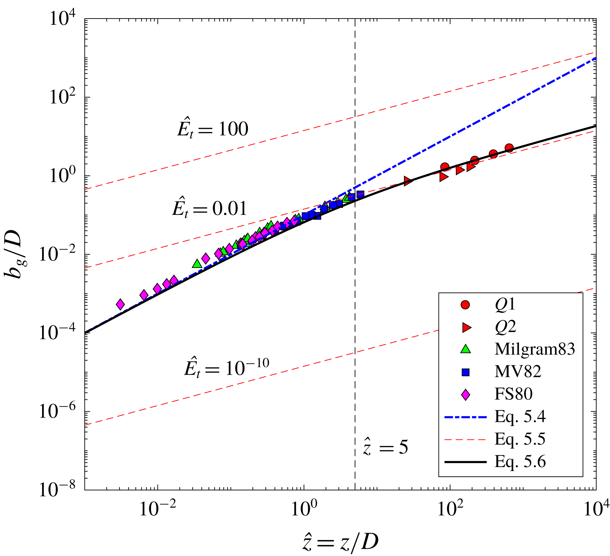


We continue the scale analysis to predict liquid volume flux $\hat{Q}$
and momentum flux
$\hat{Q}$
and momentum flux $\hat{M}$
for the classic and weak bubble plumes. For the classic bubble plume, we use the asymptotic solutions of Bombardelli et al. (Reference Bombardelli, Buscaglia, Rehmann, Rincon and Garcia2007) for
$\hat{M}$
for the classic and weak bubble plumes. For the classic bubble plume, we use the asymptotic solutions of Bombardelli et al. (Reference Bombardelli, Buscaglia, Rehmann, Rincon and Garcia2007) for $b_{g}$
and
$b_{g}$
and $U_{m}$
, presented previously here as (4.7) and (5.4). In the normalized format, we have
$U_{m}$
, presented previously here as (4.7) and (5.4). In the normalized format, we have
 $$\begin{eqnarray}\displaystyle & \displaystyle \hat{Q}=2\unicode[STIX]{x03C0}\unicode[STIX]{x1D6FD}^{2}\left(\frac{1.9\hat{z}^{5}}{1+0.563\hat{z}^{1/2}}\right)^{1/3}, & \displaystyle\end{eqnarray}$$
 $$\begin{eqnarray}\displaystyle & \displaystyle \hat{M}=2\unicode[STIX]{x03C0}\unicode[STIX]{x1D6FD}^{2}\left(\frac{1.9\hat{z}^{2}}{1+0.563\hat{z}^{1/2}}\right)^{2/3}. & \displaystyle\end{eqnarray}$$
From the weak bubble plume theory, we use (4.6) and (5.5), giving
 $$\begin{eqnarray}\displaystyle & \displaystyle \hat{Q}=6\unicode[STIX]{x03C0}\hat{E_{t}}\hat{z}^{1/2}, & \displaystyle\end{eqnarray}$$
 $$\begin{eqnarray}\displaystyle & \displaystyle \hat{M}=9\unicode[STIX]{x03C0}\hat{E_{t}}. & \displaystyle\end{eqnarray}$$
Figure 12 shows these relationships along with the measured data.

Figure 12. Non-dimensional parameters versus height in bubble plume models: (a) volume flux; (b) kinematic momentum flux. See figure 11 for data key.
Equations for classic and weak bubble plumes show significantly different behaviour in figure 12 (i.e. different power laws of the dash-dotted and dashed lines). Bombardelli et al.’s (Reference Bombardelli, Buscaglia, Rehmann, Rincon and Garcia2007) asymptotic solution tracks the volume and momentum fluxes in the classic bubble plume regime but overestimates the fluxes in the weak bubble plume regime. This is because the linear spreading theory overestimates the plume width in the weak bubble plume ( $z/D\gg 1$
). In contrast, the lines for the weak bubble plume at large
$z/D\gg 1$
). In contrast, the lines for the weak bubble plume at large $\hat{z}$
and with
$\hat{z}$
and with $\hat{E_{t}}=0.01$
are close to our data, but the data do not exactly match the slopes of these theoretical lines, with the deviation being larger for
$\hat{E_{t}}=0.01$
are close to our data, but the data do not exactly match the slopes of these theoretical lines, with the deviation being larger for $\hat{M}$
.
$\hat{M}$
.
In figures 11 and 12, the behaviour in the weak bubble plume regime is controlled by the effective diffusion coefficient, $\hat{E_{t}}$
(i.e. different dashed lines). Here we show that
$\hat{E_{t}}$
(i.e. different dashed lines). Here we show that $\hat{E_{t}}=0.01$
conforms the closest to our data for weak bubble plumes in stationary water. As discussed in § 4.1, the dimensional
$\hat{E_{t}}=0.01$
conforms the closest to our data for weak bubble plumes in stationary water. As discussed in § 4.1, the dimensional $E_{t}$
is mainly determined by the wobbling motion of these ellipsoidal bubbles. In natural and engineered gas-in-water systems, bubbles sizes are commonly in the range of 2 to 10 mm, and these bubbles have similar bubble shape, rising trajectory and rise velocity (e.g. Clift et al.
Reference Clift, Grace and Weber1978). Therefore, we expect a small variation of
$E_{t}$
is mainly determined by the wobbling motion of these ellipsoidal bubbles. In natural and engineered gas-in-water systems, bubbles sizes are commonly in the range of 2 to 10 mm, and these bubbles have similar bubble shape, rising trajectory and rise velocity (e.g. Clift et al.
Reference Clift, Grace and Weber1978). Therefore, we expect a small variation of $E_{t}$
in any weak bubble plume, and we believe that the two flow rates in our experiments created bubbles that are representative of typical cases. Likewise, slip velocity is constant near
$E_{t}$
in any weak bubble plume, and we believe that the two flow rates in our experiments created bubbles that are representative of typical cases. Likewise, slip velocity is constant near $20~\text{cm}~\text{s}^{-1}$
over a wide range of bubble sizes (Clift et al.
Reference Clift, Grace and Weber1978). Therefore, variation of the non-dimensional parameter
$20~\text{cm}~\text{s}^{-1}$
over a wide range of bubble sizes (Clift et al.
Reference Clift, Grace and Weber1978). Therefore, variation of the non-dimensional parameter $\hat{E_{t}}$
is probably caused by changes only in
$\hat{E_{t}}$
is probably caused by changes only in $D$
, or correspondingly
$D$
, or correspondingly $\hat{z}$
, and does not depend on the dimensional parameter
$\hat{z}$
, and does not depend on the dimensional parameter $E_{t}$
. For instance, when
$E_{t}$
. For instance, when $B_{0}$
decreases,
$B_{0}$
decreases, $D$
decreases, hence,
$D$
decreases, hence, $\hat{E_{t}}$
increases. Propagating this behaviour through our equations, we expect that different values of
$\hat{E_{t}}$
increases. Propagating this behaviour through our equations, we expect that different values of $\hat{E}_{t}$
will fit the data at different
$\hat{E}_{t}$
will fit the data at different $z/D$
. Hence, we might expect that, in the weak bubble plume regime, lines of constant
$z/D$
. Hence, we might expect that, in the weak bubble plume regime, lines of constant $\hat{E}_{t}$
may not track the data over large regions of
$\hat{E}_{t}$
may not track the data over large regions of $\hat{z}$
. This is consistent with our data’s deviation from the red dashed lines in figures 11 and 12.
$\hat{z}$
. This is consistent with our data’s deviation from the red dashed lines in figures 11 and 12.
The data spanning over five orders of magnitude of $\hat{z}$
show that the bubble plume follows a stable entrainment process in the classic bubble plume regime, and transitions to the weak bubble plume regime occurring near the highest value of
$\hat{z}$
show that the bubble plume follows a stable entrainment process in the classic bubble plume regime, and transitions to the weak bubble plume regime occurring near the highest value of $\hat{z}$
in our dataset, where the constant entrainment coefficient is not applicable. The non-constant entrainment coefficient and different spreading processes in two regimes show significant differences from integral model predictions using constant entrainment coefficient, and these differences are dominated by bubble lateral diffusion in the weak bubble plume regime.
$\hat{z}$
in our dataset, where the constant entrainment coefficient is not applicable. The non-constant entrainment coefficient and different spreading processes in two regimes show significant differences from integral model predictions using constant entrainment coefficient, and these differences are dominated by bubble lateral diffusion in the weak bubble plume regime.
6 Conclusion
In this paper we presented an experimental study of a weak bubble plume in a large-scale facility at two flow rates. A theory was proposed to describe the characteristics of mean flow in the weak bubble plume and was validated with the data. We also compared the weak bubble plume closely with the classic bubble plume, to examine the similarity of the two plumes and the distinct features of the weak bubble plume. In the end, we proposed a scaling framework to unify predictions for spreading rate and volume and kinematic momentum fluxes in the classic and weak bubble plume regimes, which provides insight on the transition region between them.
The weak bubble plume has Gaussian cross-sectional profiles of velocity and cross-sectional void fraction at all heights measured above our point source diffuser. Differently from the linear spreading of the classic bubble plume, the Gaussian-defined plume radius $b_{g}$
for the weak bubble plume grows following a diffusive power law
$b_{g}$
for the weak bubble plume grows following a diffusive power law $b_{g}\sim z^{1/2}$
. The growth rate is determined by the effective diffusion coefficient
$b_{g}\sim z^{1/2}$
. The growth rate is determined by the effective diffusion coefficient $E_{t}$
, which agrees with the apparent diffusion from the lateral wobbling of the rising bubbles. The contribution to this growth rate from the turbulence behind the bubble wakes is limited in stationary water. The entrainment in the weak bubble plume probably occurs in the local wake of the bubbles instead of as a shear entrainment velocity at the plume edge. The measured apparent entrainment coefficients
$E_{t}$
, which agrees with the apparent diffusion from the lateral wobbling of the rising bubbles. The contribution to this growth rate from the turbulence behind the bubble wakes is limited in stationary water. The entrainment in the weak bubble plume probably occurs in the local wake of the bubbles instead of as a shear entrainment velocity at the plume edge. The measured apparent entrainment coefficients $\unicode[STIX]{x1D6FC}$
in the weak bubble plume are not constant and correspond well with the predictive curve proposed by Milgram (Reference Milgram1983) as a function of local bubble Froude number. Theoretical analysis shows
$\unicode[STIX]{x1D6FC}$
in the weak bubble plume are not constant and correspond well with the predictive curve proposed by Milgram (Reference Milgram1983) as a function of local bubble Froude number. Theoretical analysis shows $\unicode[STIX]{x1D6FC}\sim z^{-1/2}$
in the weak bubble plume, and this decay rate is supported by the data.
$\unicode[STIX]{x1D6FC}\sim z^{-1/2}$
in the weak bubble plume, and this decay rate is supported by the data.
The centreline water velocities, scaled with bubble slip velocity, track the asymptotic solution proposed by Bombardelli et al. (Reference Bombardelli, Buscaglia, Rehmann, Rincon and Garcia2007), with $U_{m}\sim z^{-1/2}$
in the weak bubble plume. Taking the scaling laws for
$U_{m}\sim z^{-1/2}$
in the weak bubble plume. Taking the scaling laws for $b_{g}$
and
$b_{g}$
and $U_{m}$
together with the Gaussian profile, it follows that the liquid volume flux in the plume scales as
$U_{m}$
together with the Gaussian profile, it follows that the liquid volume flux in the plume scales as $Q\sim z^{m}$
where
$Q\sim z^{m}$
where $m=1/2$
. This predicts that the total liquid volume flux in the plume increases as the plume grows, but that the entrained liquid volume flux decreases with height. This is different from the single-phase plume and classic bubble plumes, which is an increasing entrainment process (i.e.
$m=1/2$
. This predicts that the total liquid volume flux in the plume increases as the plume grows, but that the entrained liquid volume flux decreases with height. This is different from the single-phase plume and classic bubble plumes, which is an increasing entrainment process (i.e. $m=5/3$
). The available data spanning classic to weak bubble plumes are bounded by
$m=5/3$
). The available data spanning classic to weak bubble plumes are bounded by $m=1/2$
and
$m=1/2$
and $5/3$
.
$5/3$
.
The classic integral models for bubble plumes do not predict the behaviour of weak bubble plumes. With the traditional constant entrainment coefficient, the classic integral model predicts the correct plume velocity but overestimates the plume width for the weak bubble plume due to its equivalent linear spreading hypothesis $b_{g}\sim z$
. Forcing a small constant entrainment coefficient in classic integral models would fail to predict the velocity of the plume. Our analysis shows that an additional parameter, the effective diffusion coefficient
$b_{g}\sim z$
. Forcing a small constant entrainment coefficient in classic integral models would fail to predict the velocity of the plume. Our analysis shows that an additional parameter, the effective diffusion coefficient $E_{t}$
, is needed to correctly predict the behaviour of the weak bubble plume.
$E_{t}$
, is needed to correctly predict the behaviour of the weak bubble plume.
Based on the data, the theory for weak bubble plumes proposed here, and the previous theory and models for classic bubble plumes, we proposed a set of non-dimensional scaling frameworks to describe the bubble plume spreading, liquid volume flux and kinematic momentum flux for the entire regime of both classic and weak bubble plumes. We expect the scaling to give insight for bubble plumes in the transition regime between classic and weak bubble plumes. The validity of this relationship in the transition regime is subject to future studies, especially in the range of $z/D\in [10,100]$
.
$z/D\in [10,100]$
.
Acknowledgements
This research was made possible by a grant from the Gulf of Mexico Research Initiative to the Gulf Integrated Spill Research (GISR) consortium, the Center for the Integrated Modeling and Analysis of the Gulf Ecosystem (C-IMAGE-II) consortium, and the project Synthesis of the Physical Processes in Subsea Bubble Plume to Connect Natural Seeps and Oil Spills (Syn-bubbles). Data are publicly available through the Gulf of Mexico Research Initiative Information & Data Cooperative (GRIIDC) at doi:10.7266/N7BP00T5 (Wang & Socolofsky Reference Wang and Socolofsky2016).
Appendix A
In this appendix, we derive the gradient of liquid volume flux for classic single-phase momentum jets, buoyant plumes and weak bubble plumes from a spreading hypothesis, which we then compare to the format of the equivalent entrainment hypothesis.
A.1 Single-phase point source momentum jet
In a self-similar pure momentum jet, the centreline velocity of the jet should be a function of $z$
and
$z$
and $M_{0}$
only, where
$M_{0}$
only, where $M_{0}$
is the initial momentum flux (Fisher et al.
Reference Fisher, List, Koh, Imberger and Brooks1979).
$M_{0}$
is the initial momentum flux (Fisher et al.
Reference Fisher, List, Koh, Imberger and Brooks1979).
Dimensional analysis gives
 $$\begin{eqnarray}U_{m}\sim \left(\frac{M_{0}}{z^{2}}\right)^{1/2}.\end{eqnarray}$$
This shows that $1/U_{m}=\unicode[STIX]{x1D6FE}z$
, where
$1/U_{m}=\unicode[STIX]{x1D6FE}z$
, where $\unicode[STIX]{x1D6FE}$
is a constant. Taking a derivative with respect to
$\unicode[STIX]{x1D6FE}$
is a constant. Taking a derivative with respect to $z$
, we obtain
$z$
, we obtain
 $$\begin{eqnarray}\frac{\text{d}U_{m}}{\text{d}z}=-\frac{U_{m}}{z}.\end{eqnarray}$$
The linear spreading hypothesis of a momentum jet gives
 $$\begin{eqnarray}\frac{\text{d}b_{g}}{\text{d}z}=\unicode[STIX]{x1D6FD}_{j}.\end{eqnarray}$$
For a point source, $b_{g}=\unicode[STIX]{x1D6FD}_{j}z$
. Therefore, equation (A 2) becomes
$b_{g}=\unicode[STIX]{x1D6FD}_{j}z$
. Therefore, equation (A 2) becomes
 $$\begin{eqnarray}\frac{\text{d}U_{m}}{\text{d}z}=-\frac{U_{m}\unicode[STIX]{x1D6FD}_{j}}{b_{g}}.\end{eqnarray}$$
Multiplying $\unicode[STIX]{x03C0}b_{g}$
to both sides of this equation yields
$\unicode[STIX]{x03C0}b_{g}$
to both sides of this equation yields
 $$\begin{eqnarray}\frac{\unicode[STIX]{x03C0}b_{g}^{2}}{U_{m}}\frac{\text{d}U_{m}}{\text{d}z}=-\unicode[STIX]{x03C0}\unicode[STIX]{x1D6FD}_{j}b_{g}.\end{eqnarray}$$
Moving $\unicode[STIX]{x03C0}b_{g}^{2}$
inside of the derivative, with
$\unicode[STIX]{x03C0}b_{g}^{2}$
inside of the derivative, with $Q=\unicode[STIX]{x03C0}b_{g}^{2}U_{m}$
, we have
$Q=\unicode[STIX]{x03C0}b_{g}^{2}U_{m}$
, we have
 $$\begin{eqnarray}\frac{\text{d}Q}{\text{d}z}=\unicode[STIX]{x03C0}\unicode[STIX]{x1D6FD}_{j}b_{g}U_{m}.\end{eqnarray}$$
This is equivalent to the entrainment hypothesis, i.e. equation (4.10), and we have $\unicode[STIX]{x1D6FC}=\unicode[STIX]{x1D6FD}_{j}/2$
.
$\unicode[STIX]{x1D6FC}=\unicode[STIX]{x1D6FD}_{j}/2$
.
A.2 Single-phase point source buoyant plume
In a self-similar pure buoyant plume, the centreline velocity of the plume should be a function of $z$
and
$z$
and $B_{0}$
only, where
$B_{0}$
only, where $B_{0}$
is the initial buoyancy flux.
$B_{0}$
is the initial buoyancy flux.
Dimensional analysis gives
 $$\begin{eqnarray}U_{m}\sim \left(\frac{B_{0}}{z}\right)^{1/3}.\end{eqnarray}$$
This shows that $1/U_{m}=\unicode[STIX]{x1D6FE}z^{1/3}$
, where
$1/U_{m}=\unicode[STIX]{x1D6FE}z^{1/3}$
, where $\unicode[STIX]{x1D6FE}$
is a constant. Taking the
$\unicode[STIX]{x1D6FE}$
is a constant. Taking the $z$
derivative, we obtain
$z$
derivative, we obtain
 $$\begin{eqnarray}\frac{\text{d}U_{m}}{\text{d}z}=-\frac{1}{3}\frac{U_{m}}{z}.\end{eqnarray}$$
Note that this equation is in the same format as the equation for a jet (i.e. equation (A 2)).
We still have a linear spreading hypothesis in the single-phase plume. Following the same procedure for the plume from (A 3) to (A 6), we can derive the gradient of the liquid volume flux for a single-phase point source plume as
 $$\begin{eqnarray}\frac{\text{d}Q}{\text{d}z}=\frac{5}{3}\unicode[STIX]{x03C0}\unicode[STIX]{x1D6FD}_{p}b_{g}U_{m}.\end{eqnarray}$$
This is also equivalent to the entrainment hypothesis (4.10), and we have $\unicode[STIX]{x1D6FC}=5\unicode[STIX]{x1D6FD}_{p}/6$
.
$\unicode[STIX]{x1D6FC}=5\unicode[STIX]{x1D6FD}_{p}/6$
.
A.3 Weak point source bubble plume
In weak bubble plumes, the centreline velocity of the plume should be a function of $z$
,
$z$
, $E_{t}$
,
$E_{t}$
, $B_{0}$
and
$B_{0}$
and $U_{s}$
. Bombardelli et al. (Reference Bombardelli, Buscaglia, Rehmann, Rincon and Garcia2007) showed (see (4.6)) that
$U_{s}$
. Bombardelli et al. (Reference Bombardelli, Buscaglia, Rehmann, Rincon and Garcia2007) showed (see (4.6)) that
 $$\begin{eqnarray}U_{m}\sim U_{s}\left(\frac{z}{D}\right)^{-1/2}.\end{eqnarray}$$
This shows that $1/U_{m}=\unicode[STIX]{x1D6FE}z^{1/2}$
, where
$1/U_{m}=\unicode[STIX]{x1D6FE}z^{1/2}$
, where $\unicode[STIX]{x1D6FE}$
is a constant. Taking the
$\unicode[STIX]{x1D6FE}$
is a constant. Taking the $z$
derivative, we obtain
$z$
derivative, we obtain
 $$\begin{eqnarray}\frac{\text{d}U_{m}}{\text{d}z}=-\frac{1}{2}\frac{U_{m}}{z}.\end{eqnarray}$$
This equation follows the same format as those in single-phase jets and plumes (i.e. equations (A 2) and (A 8)).
Differently from single-phase jets and plumes, the development of the weak bubble plume follows a diffusive spreading instead of linear spreading process, namely
 $$\begin{eqnarray}\frac{\text{d}b_{g}^{2}}{\text{d}z}=\unicode[STIX]{x1D6FD}_{b},\end{eqnarray}$$
where $\unicode[STIX]{x1D6FD}_{b}=2E_{t}/U_{s}$
is a constant. For a point source, we have
$\unicode[STIX]{x1D6FD}_{b}=2E_{t}/U_{s}$
is a constant. For a point source, we have $z=b_{g}^{2}/\unicode[STIX]{x1D6FD}_{b}$
, which can be substituted in (A 11) to give
$z=b_{g}^{2}/\unicode[STIX]{x1D6FD}_{b}$
, which can be substituted in (A 11) to give
 $$\begin{eqnarray}\frac{\text{d}U_{m}}{\text{d}z}=-\frac{1}{2}\frac{U_{m}\unicode[STIX]{x1D6FD}_{b}}{b_{g}^{2}}.\end{eqnarray}$$
Multiplying $\unicode[STIX]{x03C0}b_{g}$
to both sides of this equation and reorganizing gives
$\unicode[STIX]{x03C0}b_{g}$
to both sides of this equation and reorganizing gives
 $$\begin{eqnarray}\frac{\text{d}Q}{\text{d}z}=\frac{1}{2}\unicode[STIX]{x03C0}\unicode[STIX]{x1D6FD}_{b}U_{m}.\end{eqnarray}$$
This equation is not in the format of the entrainment hypothesis, as $b_{g}$
is missing from the right-hand side of the equation, and
$b_{g}$
is missing from the right-hand side of the equation, and $\unicode[STIX]{x1D6FD}_{b}$
is of dimension
$\unicode[STIX]{x1D6FD}_{b}$
is of dimension ${\mathcal{L}}$
. We discuss the physical interpretation of (A 14) in § 4.4.
${\mathcal{L}}$
. We discuss the physical interpretation of (A 14) in § 4.4.


