


1 Introduction
In order to satisfy the nonlinear kinematic and dynamic free-surface boundary conditions, linear freely propagating surface gravity waves are accompanied by nonlinear bound components. For periodic waves, a so-called Stokes expansion in the amplitude of the waves reveals that any periodic wave is accompanied by a series of harmonic components with integer multiples of the frequency of the linear parent wave and their magnitude proportional to increasing integer powers of the steepness (Stokes Reference Stokes1847). For multichromatic parent waves representing wave groups, the harmonic components interact to give both ‘frequency-sum’ and ‘frequency-difference’ terms, as first described by Longuet-Higgins & Stewart (Reference Longuet-Higgins and Stewart1962) for unidirectional waves and to second order in steepness. Although expressions for the frequency-difference terms in a multidirectional sea can be distilled from Hasselmann (Reference Hasselmann1962) (cf. Okihiro, Guza & Seymour Reference Okihiro, Guza and Seymour1992), Sharma & Dean (Reference Sharma and Dean1981), Dalzell (Reference Dalzell1999) and Forristall (Reference Forristall2000) are commonly credited for extending the work of Longuet-Higgins & Stewart (Reference Longuet-Higgins and Stewart1962) to directional seas, allowing for interactions between parent wave components of different frequencies and travelling in different directions (see Pellet et al. (Reference Pellet, Christodoulides, Donne, Bean and Dias2017) for a recent rederivation that also includes pressure). In the limit of a quasimonochromatic group with a single carrier wave travelling in one direction, differential equations describing these second-order bound interactions can also be calculated using a multiple-scale approach. In the seminal papers by Dysthe (Reference Dysthe1979) (infinite water depth) and Davey & Stewartson (Reference Davey and Stewartson1974) (finite water depth), the nonlinear evolution equations for the wave group are accompanied by a second set of differential equations describing the mean flow and the wave-averaged free surface.
Physically, in the unidirectional case, the bound frequency-difference terms cause a depression in the wave-averaged surface elevation on the scale of the wave group, often referred to as a set-down (Longuet-Higgins & Stewart Reference Longuet-Higgins and Stewart1962). It can be thought of as the free-surface manifestation of the return flow underneath the group that forms to balance the Stokes transport, which is divergent on the scale of the group and acts to ‘pump’ fluid from its trailing edge to its leading edge (McIntyre Reference McIntyre1981; van den Bremer & Taylor Reference van den Bremer and Taylor2015, Reference van den Bremer and Taylor2016). In the classical interpretation, the return flow is driven by a gradient in the radiation stresses (Longuet-Higgins & Stewart Reference Longuet-Higgins and Stewart1964). The set-down is simply largest at the centre of the group, where the (negative) return flow is also largest in magnitude. In the limit of a unidirectional deep-water parent wave and a group that is long relative to the water depth $d$
, the set-down becomes (Longuet-Higgins & Stewart Reference Longuet-Higgins and Stewart1964)
$d$
, the set-down becomes (Longuet-Higgins & Stewart Reference Longuet-Higgins and Stewart1964)
 $$\begin{eqnarray}\unicode[STIX]{x1D702}_{-}^{(2)}=-\frac{|A(\tilde{x})|^{2}}{4d},\end{eqnarray}$$
where $A$
denotes the amplitude envelope of the group and
$A$
denotes the amplitude envelope of the group and $\tilde{x}=x-c_{g,0}t$
is the horizontal coordinate in the group reference frame. We will briefly review the derivation of (1.1) in § 2.
$\tilde{x}=x-c_{g,0}t$
is the horizontal coordinate in the group reference frame. We will briefly review the derivation of (1.1) in § 2.
However, when examining the very large freak wave that occurred at the Draupner Platform in the North Sea on 1 January 1995, Walker, Taylor & Eatock Taylor (Reference Walker, Taylor and Eatock Taylor2004) observed a large set-up in the wave-averaged surface elevation. Subsequent analysis of the Draupner wave by Adcock & Taylor (Reference Adcock and Taylor2009) and Adcock et al. (Reference Adcock, Taylor, Yan, Ma and Janssen2011) identified crossing waves as the probable cause of the set-up associated with the Draupner wave. This finding is supported by a high-resolution hindcast model of the Draupner storm performed by Cavaleri et al. (Reference Cavaleri, Barbariol, Benetazzo, Bertotti, Bidlot, Janssen and Wedi2016), which highlighted the presence of two large crossing wave systems. In addition to Draupner, Fedele et al. (Reference Fedele, Brennan, De León, Dudley and Dias2016) examined set-up in the wave-averaged surface elevation of two other very large wave events, concluding that crossing directional spectra were the likely cause. The set-up of the wave-averaged free surface in crossing seas can thus be seen as an important contribution to the crest height of freak waves (see Kharif & Pelinovsky (Reference Kharif and Pelinovsky2003), Dysthe, Müller & Krogstad (Reference Dysthe, Müller and Krogstad2008), Onorato et al. (Reference Onorato, Residori, Bortolozzo, Montina and Arecchi2013) and Adcock & Taylor (Reference Adcock and Taylor2014) for reviews of the mechanisms behind freak waves). We specifically do not examine herein the possible (enhanced) occurrence of modulational or Benjamin–Feir instability in crossing seas, as might be described by coupled nonlinear Schrödinger equations (e.g. Onorato, Osborne & Serio (Reference Onorato, Osborne and Serio2006) and references therein).
A set-up was also observed by Toffoli et al. (Reference Toffoli, Monbaliu, Onorato, Osborne, Babanin and Bitner-Gregersen2007) for smaller waves measured on Lake George, Australia. Toffoli et al. (Reference Toffoli, Monbaliu, Onorato, Osborne, Babanin and Bitner-Gregersen2007) showed this effect to be consistent with second-order theory, and found that crossing waves of similar frequency result in positive interaction by numerically computing the frequency-difference interaction kernel of Sharma & Dean (Reference Sharma and Dean1981). These effects were also observed in time-domain simulations performed by Toffoli, Onorato & Monbaliu (Reference Toffoli, Onorato and Monbaliu2006). A similar observation was made by Okihiro et al. (Reference Okihiro, Guza and Seymour1992) based on the (equivalent) frequency-difference interaction kernel reconstructed from Hasselmann (Reference Hasselmann1962), noting that this kernel reduces with increasing angle and changes sign for two wave components at an angle of $30^{\circ }$
in deep water (
$30^{\circ }$
in deep water ( $k_{0}d\gg 1$
). Indeed, the energy spectrum associated with second-order bound waves reduces considerably with increasing directional spreading (Herbers, Elgar & Guza Reference Herbers, Elgar and Guza1994). Recently, Herbers & Janssen (Reference Herbers and Janssen2016) have shown that the set-down associated with (unidirectional) groups can appear as a significant set-up in Lagrangian buoy records, emphasizing the need to carefully distinguish between Lagrangian and Eulerian field observations.
$k_{0}d\gg 1$
). Indeed, the energy spectrum associated with second-order bound waves reduces considerably with increasing directional spreading (Herbers, Elgar & Guza Reference Herbers, Elgar and Guza1994). Recently, Herbers & Janssen (Reference Herbers and Janssen2016) have shown that the set-down associated with (unidirectional) groups can appear as a significant set-up in Lagrangian buoy records, emphasizing the need to carefully distinguish between Lagrangian and Eulerian field observations.
Experimentally, Johannessen & Swan (Reference Johannessen and Swan2001) examined the evolution and focusing of moderately directionally spread focused wave groups and found that the directionality of the wave groups serves to reduce the overall nonlinearity of the waves, affecting the onset of breaking and nonlinear modification of the free waves. Onorato et al. (Reference Onorato, Cavaleri, Fouques, Gramstad, Janssen, Monbaliu, Osborne, Pakozdi, Serio and Stansberg2009) and Toffoli et al. (Reference Toffoli, Gramstad, Monbaliu, Trulsen, Bitner-Gregersen and Onorato2010) performed experiments and numerical analysis of irregular crossing waves, observing a direct relationship between crossing angle and kurtosis, an indicator of the probability of freak wave occurrence. All of the experimental studies that we are aware of have been limited to small degrees of directional spreading and have not observed the formation of a set-up, with the exception of Toffoli et al. (Reference Toffoli, Bitner-Gregersen, Osborne, Serio, Monbaliu and Onorato2011), who did conduct experiments with crossing wave systems at crossing angles up to $40^{\circ }$
, but did not specifically examine the occurrence of a set-up.
$40^{\circ }$
, but did not specifically examine the occurrence of a set-up.
Herein, we examine the structure and magnitude of the wave-averaged free surface for directionally spread and crossing surface gravity wave groups through a combination of multiple-scale expansions and physical experiments for all possible degrees of spreading. We investigate when a set-down can turn into a set-up. Our experiments are conducted in the circular wave tank at the FloWave Ocean Energy Research Facility at the University of Edinburgh (see Ingram et al. (Reference Ingram, Wallace, Robinson and Bryden2014) for details of the facility). This has 168 individually controlled paddles, enabling the generation of wave groups with any desired directional distribution. We carry out two categories of experiments: tests in which we vary the degree of directional spreading for an individual wave group (category A) and tests in which we let two wave groups cross each other at different angles (category B). Figure 1 illustrates the linear surface profile at the time of linear focus for the groups we examine experimentally in category A, showing specifically three individual groups of increasing degree of directional spreading. Figure 2 shows the perfectly focused predicted linear surface profile for two groups with narrow individual degrees of directional spreading crossing at an angle, as examined in category B.
This paper is laid out as follows. First, in § 2, we present our multiple-scale solutions for crossing groups and review existing second-order theory. In § 3, we outline our experimental method and introduce the two types of experiments we perform. We compare our experimental results with theory in § 4. Finally, conclusions are drawn in § 5.

Figure 1. Illustration of the linear surface profile $\unicode[STIX]{x1D702}^{(1)}(x,y,t=0)$
for spreading and surface tests (category A) at time of focus (
$\unicode[STIX]{x1D702}^{(1)}(x,y,t=0)$
for spreading and surface tests (category A) at time of focus ( $t=0$
) and for three different degrees of spreading,
$t=0$
) and for three different degrees of spreading, $\unicode[STIX]{x1D70E}_{\unicode[STIX]{x1D703}}=10,20,30^{\circ }$
. (a–c) The surfaces and (d–f) the corresponding contours, showing positive contours only for clarity (linear amplitude at focus
$\unicode[STIX]{x1D70E}_{\unicode[STIX]{x1D703}}=10,20,30^{\circ }$
. (a–c) The surfaces and (d–f) the corresponding contours, showing positive contours only for clarity (linear amplitude at focus $a_{0}=0.1~\text{m}$
for a perfectly focused linear group). The colour bar applies to (d–f) only.
$a_{0}=0.1~\text{m}$
for a perfectly focused linear group). The colour bar applies to (d–f) only.
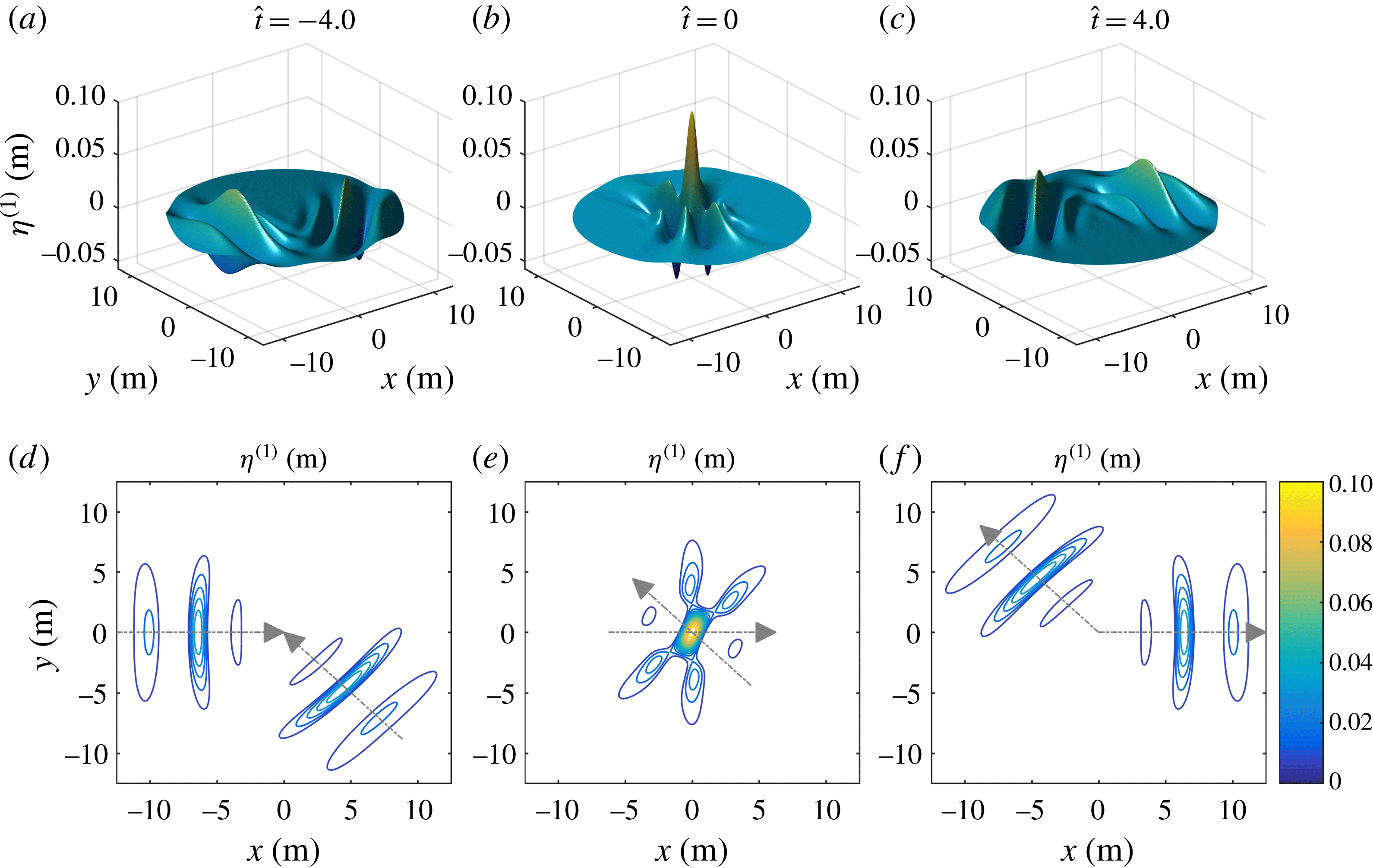
Figure 2. Illustration of the linear surface profile $\unicode[STIX]{x1D702}^{(1)}(x,y,t)$
for crossing tests (category B), showing two wave groups with moderate degrees of directional spreading (
$\unicode[STIX]{x1D702}^{(1)}(x,y,t)$
for crossing tests (category B), showing two wave groups with moderate degrees of directional spreading ( $\unicode[STIX]{x1D70E}_{\unicode[STIX]{x1D703}}=10^{\circ }$
) at a crossing angle of
$\unicode[STIX]{x1D70E}_{\unicode[STIX]{x1D703}}=10^{\circ }$
) at a crossing angle of $\unicode[STIX]{x0394}\unicode[STIX]{x1D703}=135^{\circ }$
for three different times,
$\unicode[STIX]{x0394}\unicode[STIX]{x1D703}=135^{\circ }$
for three different times, $\hat{t}\equiv c_{g,0}t/\unicode[STIX]{x1D70E}_{x}$
: before focus at
$\hat{t}\equiv c_{g,0}t/\unicode[STIX]{x1D70E}_{x}$
: before focus at $\hat{t}=-4.0$
(a,d), at linear focus
$\hat{t}=-4.0$
(a,d), at linear focus $\hat{t}=0$
(b,e) and after focus at
$\hat{t}=0$
(b,e) and after focus at $\hat{t}=4.0$
(c,f); (a–c) display the linear surfaces and (d–f) the corresponding contours, showing positive contours only for clarity (combined linear amplitude at focus
$\hat{t}=4.0$
(c,f); (a–c) display the linear surfaces and (d–f) the corresponding contours, showing positive contours only for clarity (combined linear amplitude at focus $a_{0}=0.1~\text{m}$
). The colour bar applies to (d–f) only.
$a_{0}=0.1~\text{m}$
). The colour bar applies to (d–f) only.
2 Second-order theory
In this section, we use a multiple-scale approach to gain insight into the mechanisms behind the formation of the set-down or set-up of the wave-averaged free surface and their relative magnitudes under different circumstances. We begin by briefly reviewing the governing equations and boundary conditions in § 2.1, followed by a discussion of the set-down formed for a single narrowly spread group in § 2.2 and the formation of a set-up when two groups cross each other at an angle in § 2.3. Finally, in § 2.4, we compare our simple expressions for the set-down and set-up with the explicitly computed wave-averaged free-surface elevation from existing second-order theory based on the component-by-component interaction of individual waves with different frequencies and directions.
2.1 Governing equations
A three-dimensional body of water of depth $d$
and indefinite lateral extent is assumed with a coordinate system (
$d$
and indefinite lateral extent is assumed with a coordinate system ( $x$
,
$x$
, $y$
,
$y$
, $z$
), where
$z$
), where $x$
and
$x$
and $y$
denote the horizontal coordinates and
$y$
denote the horizontal coordinates and $z$
the vertical coordinate measured from the undisturbed water level upwards. Inviscid, incompressible and irrotational flow is assumed and, as a result, the velocity vector can be defined as the gradient of the velocity potential,
$z$
the vertical coordinate measured from the undisturbed water level upwards. Inviscid, incompressible and irrotational flow is assumed and, as a result, the velocity vector can be defined as the gradient of the velocity potential, $\boldsymbol{u}=\unicode[STIX]{x1D735}\unicode[STIX]{x1D719}$
. The governing equation within the domain of the fluid is then Laplace,
$\boldsymbol{u}=\unicode[STIX]{x1D735}\unicode[STIX]{x1D719}$
. The governing equation within the domain of the fluid is then Laplace,
 $$\begin{eqnarray}\unicode[STIX]{x1D6FB}^{2}\unicode[STIX]{x1D719}=0\quad \text{for}~-d\leqslant z\leqslant \unicode[STIX]{x1D702}(x,y,t),\end{eqnarray}$$
where $\unicode[STIX]{x1D702}(x,y,t)$
denotes the free surface. The kinematic and dynamic free-surface boundary conditions are respectively
$\unicode[STIX]{x1D702}(x,y,t)$
denotes the free surface. The kinematic and dynamic free-surface boundary conditions are respectively
 $$\begin{eqnarray}w-\frac{\unicode[STIX]{x2202}\unicode[STIX]{x1D702}}{\unicode[STIX]{x2202}t}-u\frac{\unicode[STIX]{x2202}\unicode[STIX]{x1D702}}{\unicode[STIX]{x2202}x}-v\frac{\unicode[STIX]{x2202}\unicode[STIX]{x1D702}}{\unicode[STIX]{x2202}y}=0,\quad g\unicode[STIX]{x1D702}+\frac{\unicode[STIX]{x2202}\unicode[STIX]{x1D719}}{\unicode[STIX]{x2202}t}+\frac{1}{2}|\unicode[STIX]{x1D735}\unicode[STIX]{x1D719}|^{2}=0\quad \text{at }z=\unicode[STIX]{x1D702}(x,y,t),\end{eqnarray}$$
where gravity $g$
acts in the negative
$g$
acts in the negative $z$
direction and
$z$
direction and $|\unicode[STIX]{x1D735}\unicode[STIX]{x1D719}|^{2}=u^{2}+v^{2}+w^{2}$
. Finally, there is a no-flow bottom boundary condition, requiring that
$|\unicode[STIX]{x1D735}\unicode[STIX]{x1D719}|^{2}=u^{2}+v^{2}+w^{2}$
. Finally, there is a no-flow bottom boundary condition, requiring that $\unicode[STIX]{x2202}\unicode[STIX]{x1D719}/\unicode[STIX]{x2202}z=0$
at
$\unicode[STIX]{x2202}\unicode[STIX]{x1D719}/\unicode[STIX]{x2202}z=0$
at $z=-d$
. By retaining terms up to quadratic in the amplitude of the waves, the two free-surface boundary conditions in (2.2) can be combined into two forcing equations for the mean flow and the wave-averaged free surface respectively,
$z=-d$
. By retaining terms up to quadratic in the amplitude of the waves, the two free-surface boundary conditions in (2.2) can be combined into two forcing equations for the mean flow and the wave-averaged free surface respectively,
 $$\begin{eqnarray}\displaystyle & \displaystyle \left.\left(\frac{\unicode[STIX]{x2202}}{\unicode[STIX]{x2202}z}+\frac{1}{g}\frac{\unicode[STIX]{x2202}^{2}}{\unicode[STIX]{x2202}t^{2}}\right)\unicode[STIX]{x1D719}_{-}^{(2)}\right|_{z=0}=\overline{\unicode[STIX]{x1D735}_{H}\boldsymbol{\cdot }(\boldsymbol{u}_{H}^{(1)}|_{z=0}\unicode[STIX]{x1D702}^{(1)})-\frac{1}{g}\frac{\unicode[STIX]{x2202}}{\unicode[STIX]{x2202}t}\left(\left.\frac{\unicode[STIX]{x2202}^{2}\unicode[STIX]{x1D719}^{(1)}}{\unicode[STIX]{x2202}z\unicode[STIX]{x2202}t}\right|_{z=0}\unicode[STIX]{x1D702}^{(1)}+\frac{1}{2}|\unicode[STIX]{x1D735}\unicode[STIX]{x1D719}|_{z=0}^{2}\right)}, & \displaystyle\end{eqnarray}$$
 $$\begin{eqnarray}\displaystyle & \displaystyle \unicode[STIX]{x1D702}_{-}^{(2)}=\frac{-1}{g}\left(\left.\frac{\unicode[STIX]{x2202}\unicode[STIX]{x1D719}_{-}^{(2)}}{\unicode[STIX]{x2202}t}\right|_{z=0}+\overline{\left(\left.\frac{\unicode[STIX]{x2202}^{2}\unicode[STIX]{x1D719}^{(1)}}{\unicode[STIX]{x2202}z\unicode[STIX]{x2202}t}\right|_{z=0}\unicode[STIX]{x1D702}^{(1)}+\left.\frac{1}{2}|\unicode[STIX]{x1D735}\unicode[STIX]{x1D719}|^{2}\right|_{z=0}\right)}\right), & \displaystyle\end{eqnarray}$$
where the superscripts denote the order in amplitude and the subscripts signify that we only retain wave-averaged terms here, as also indicated by the overlines on the right-hand side. We specify our definition of wave-averaging below. Finally, the subscript $H$
denotes horizontal components only, so that
$H$
denotes horizontal components only, so that $\boldsymbol{u}_{H}=(u,v,0)$
.
$\boldsymbol{u}_{H}=(u,v,0)$
.
2.2 A single narrow-banded and narrowly spread wave group: set-down
We first consider a single wave group travelling in the positive $x$
direction, which has the linear signal
$x$
direction, which has the linear signal
 $$\begin{eqnarray}\unicode[STIX]{x1D702}^{(1)}=Re[A(X,Y)\text{e}^{\text{i}(k_{0}x-\unicode[STIX]{x1D714}_{0}t)}],\quad \unicode[STIX]{x1D719}^{(1)}=Re\left[-\text{i}\frac{\unicode[STIX]{x1D714}_{0}}{k_{0}}A(X,Y)\text{e}^{k_{0}z+\text{i}(k_{0}x-\unicode[STIX]{x1D714}_{0}t)}\right],\end{eqnarray}$$
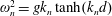
where we have assumed that the linear wave is short relative to the water depth, so that $k_{0}d\gg 1$
, as in the rest of this paper and for the experiments we perform. We will refer to this assumption as deep water, although the water depth is not truly infinite, and, in fact, it is shallow to intermediate relative to the spatial extent of the group. The linear dispersion relationship becomes
$k_{0}d\gg 1$
, as in the rest of this paper and for the experiments we perform. We will refer to this assumption as deep water, although the water depth is not truly infinite, and, in fact, it is shallow to intermediate relative to the spatial extent of the group. The linear dispersion relationship becomes $\unicode[STIX]{x1D714}_{0}^{2}=gk_{0}$
, and the prefactor on
$\unicode[STIX]{x1D714}_{0}^{2}=gk_{0}$
, and the prefactor on $\unicode[STIX]{x1D719}^{(1)}$
has been chosen so that the linearized boundary conditions (2.2) are satisfied. To leading-order in the multiple-scale parameter
$\unicode[STIX]{x1D719}^{(1)}$
has been chosen so that the linearized boundary conditions (2.2) are satisfied. To leading-order in the multiple-scale parameter $\unicode[STIX]{x1D716}_{x}\equiv 1/(k_{0}\unicode[STIX]{x1D70E}_{x})$
, with
$\unicode[STIX]{x1D716}_{x}\equiv 1/(k_{0}\unicode[STIX]{x1D70E}_{x})$
, with $\unicode[STIX]{x1D70E}_{x}$
denoting the characteristic spatial scale of the group in its direction of propagation, the group is a function of the slow variables,
$\unicode[STIX]{x1D70E}_{x}$
denoting the characteristic spatial scale of the group in its direction of propagation, the group is a function of the slow variables, $X\equiv \unicode[STIX]{x1D716}_{x}(x-c_{g,0}t)$
and
$X\equiv \unicode[STIX]{x1D716}_{x}(x-c_{g,0}t)$
and $Y\equiv \unicode[STIX]{x1D716}_{y}y$
, where
$Y\equiv \unicode[STIX]{x1D716}_{y}y$
, where $c_{g,0}=\text{d}\unicode[STIX]{x1D714}_{0}/\text{d}k_{0}=\unicode[STIX]{x1D714}_{0}/(2k_{0})$
is the group velocity. We define
$c_{g,0}=\text{d}\unicode[STIX]{x1D714}_{0}/\text{d}k_{0}=\unicode[STIX]{x1D714}_{0}/(2k_{0})$
is the group velocity. We define $\unicode[STIX]{x1D716}_{y}\equiv 1/(k_{0}\unicode[STIX]{x1D70E}_{y})$
and set
$\unicode[STIX]{x1D716}_{y}\equiv 1/(k_{0}\unicode[STIX]{x1D70E}_{y})$
and set $O(\unicode[STIX]{x1D716}_{y})=O(\unicode[STIX]{x1D716}_{x})$
or smaller. The case
$O(\unicode[STIX]{x1D716}_{y})=O(\unicode[STIX]{x1D716}_{x})$
or smaller. The case $\unicode[STIX]{x1D716}_{y}=\unicode[STIX]{x1D716}_{x}$
corresponds to a round envelope (
$\unicode[STIX]{x1D716}_{y}=\unicode[STIX]{x1D716}_{x}$
corresponds to a round envelope ( $\unicode[STIX]{x1D70E}_{y}=\unicode[STIX]{x1D70E}_{x}$
) and
$\unicode[STIX]{x1D70E}_{y}=\unicode[STIX]{x1D70E}_{x}$
) and $\unicode[STIX]{x1D716}_{y}\rightarrow 0$
to a long-crested or unidirectional wave group. By transforming into the reference frame of the group, neglecting the higher-order (in
$\unicode[STIX]{x1D716}_{y}\rightarrow 0$
to a long-crested or unidirectional wave group. By transforming into the reference frame of the group, neglecting the higher-order (in $\unicode[STIX]{x1D716}_{x}$
) double time derivative on the left-hand side of (2.3) and substituting the linear solutions (2.5) on the right-hand side, the mean flow forcing equation (2.3) becomes, after averaging over the fast temporal scales (cf. Dysthe Reference Dysthe1979),
$\unicode[STIX]{x1D716}_{x}$
) double time derivative on the left-hand side of (2.3) and substituting the linear solutions (2.5) on the right-hand side, the mean flow forcing equation (2.3) becomes, after averaging over the fast temporal scales (cf. Dysthe Reference Dysthe1979),
 $$\begin{eqnarray}\left.\frac{\unicode[STIX]{x2202}\unicode[STIX]{x1D719}_{-}^{(2)}}{\unicode[STIX]{x2202}z}\right|_{z=0}=\frac{1}{2}\unicode[STIX]{x1D714}_{0}\unicode[STIX]{x1D716}_{x}\unicode[STIX]{x2202}_{X}|A|^{2},\end{eqnarray}$$
where only the divergence of the Stokes transport $\overline{\unicode[STIX]{x1D735}_{H}\boldsymbol{\cdot }(\boldsymbol{u}_{H}^{(1)}(z=0)\unicode[STIX]{x1D702}^{(1)})}$
on the right-hand side of (2.3) contributes for deep water (
$\overline{\unicode[STIX]{x1D735}_{H}\boldsymbol{\cdot }(\boldsymbol{u}_{H}^{(1)}(z=0)\unicode[STIX]{x1D702}^{(1)})}$
on the right-hand side of (2.3) contributes for deep water ( $k_{0}d\gg 1$
), and a small degree of directional spreading is captured by the slow variation of the envelope in the direction normal to propagation (
$k_{0}d\gg 1$
), and a small degree of directional spreading is captured by the slow variation of the envelope in the direction normal to propagation ( $Y$
). For quasimonochromatic wave groups, the problem is steady, and the return flow is simply the irrotational and incompressible response to the divergence of the Stokes transport (cf. ‘Stokes pumping’) in the reference frame of the group, as is well known (see van den Bremer & Taylor (Reference van den Bremer and Taylor2016) for a discussion of the generally small effects of dispersion and a comparison of the multiple-scale solution with the original solution of Longuet-Higgins & Stewart (Reference Longuet-Higgins and Stewart1962)). Solution of the Laplace equation
$Y$
). For quasimonochromatic wave groups, the problem is steady, and the return flow is simply the irrotational and incompressible response to the divergence of the Stokes transport (cf. ‘Stokes pumping’) in the reference frame of the group, as is well known (see van den Bremer & Taylor (Reference van den Bremer and Taylor2016) for a discussion of the generally small effects of dispersion and a comparison of the multiple-scale solution with the original solution of Longuet-Higgins & Stewart (Reference Longuet-Higgins and Stewart1962)). Solution of the Laplace equation $\unicode[STIX]{x1D6FB}^{2}\unicode[STIX]{x1D719}_{-}^{(2)}=0$
, subject to the bottom boundary condition and the forcing equation (2.6) in Fourier space, gives after averaging over the fast temporal scales (cf. van den Bremer & Taylor Reference van den Bremer and Taylor2015)
$\unicode[STIX]{x1D6FB}^{2}\unicode[STIX]{x1D719}_{-}^{(2)}=0$
, subject to the bottom boundary condition and the forcing equation (2.6) in Fourier space, gives after averaging over the fast temporal scales (cf. van den Bremer & Taylor Reference van den Bremer and Taylor2015)
 $$\begin{eqnarray}\unicode[STIX]{x1D719}_{-}^{(2)}=\frac{\text{i}\unicode[STIX]{x1D714}_{0}|a_{0}|^{2}\unicode[STIX]{x1D70E}_{x}\unicode[STIX]{x1D70E}_{y}}{8\unicode[STIX]{x03C0}}\int _{-\infty }^{\infty }\int _{-\infty }^{\infty }\frac{\unicode[STIX]{x1D705}\cosh (\sqrt{\unicode[STIX]{x1D705}^{2}+\unicode[STIX]{x1D706}^{2}}(z+d))}{\sqrt{\unicode[STIX]{x1D705}^{2}+\unicode[STIX]{x1D706}^{2}}\sinh (\sqrt{\unicode[STIX]{x1D705}^{2}+\unicode[STIX]{x1D706}^{2}}d)}\text{e}^{-(\unicode[STIX]{x1D705}\unicode[STIX]{x1D70E}_{x})^{2}/4-(\unicode[STIX]{x1D706}\unicode[STIX]{x1D70E}_{y})^{2}/4}\text{e}^{\text{i}(\unicode[STIX]{x1D705}\tilde{x}+\unicode[STIX]{x1D706}{\tilde{y}})}\,\text{d}\unicode[STIX]{x1D705}\,\text{d}\unicode[STIX]{x1D706},\end{eqnarray}$$
where we have chosen a Gaussian envelope, $A=a_{0}\exp (-\tilde{x}^{2}/(2\unicode[STIX]{x1D70E}_{x}^{2})-{\tilde{y}}^{2}/(2\unicode[STIX]{x1D70E}_{y}^{2}))$
, with
$A=a_{0}\exp (-\tilde{x}^{2}/(2\unicode[STIX]{x1D70E}_{x}^{2})-{\tilde{y}}^{2}/(2\unicode[STIX]{x1D70E}_{y}^{2}))$
, with $\tilde{x}=x-c_{g,0}t$
and
$\tilde{x}=x-c_{g,0}t$
and ${\tilde{y}}=y$
, for illustrative purposes. Turning to the wave-averaged surface forcing equation (2.4), it can be shown by substituting the linear solutions (2.5) on the right-hand side that, for a single wave group in deep water (
${\tilde{y}}=y$
, for illustrative purposes. Turning to the wave-averaged surface forcing equation (2.4), it can be shown by substituting the linear solutions (2.5) on the right-hand side that, for a single wave group in deep water ( $k_{0}d\gg 1$
), only the mean flow term (
$k_{0}d\gg 1$
), only the mean flow term ( $-(1/g)\unicode[STIX]{x2202}\unicode[STIX]{x1D719}_{-}^{(2)}/\unicode[STIX]{x2202}t$
) makes a non-zero contribution. Transforming into the group reference frame and substituting (2.7), equation (2.4) becomes
$-(1/g)\unicode[STIX]{x2202}\unicode[STIX]{x1D719}_{-}^{(2)}/\unicode[STIX]{x2202}t$
) makes a non-zero contribution. Transforming into the group reference frame and substituting (2.7), equation (2.4) becomes
 $$\begin{eqnarray}\unicode[STIX]{x1D702}_{-}^{(2)}=\frac{-|a_{0}|^{2}\unicode[STIX]{x1D70E}_{x}\unicode[STIX]{x1D70E}_{y}}{16\unicode[STIX]{x03C0}}\int _{-\infty }^{\infty }\int _{-\infty }^{\infty }\frac{\unicode[STIX]{x1D705}^{2}}{\sqrt{\unicode[STIX]{x1D705}^{2}+\unicode[STIX]{x1D706}^{2}}\tanh (\sqrt{\unicode[STIX]{x1D705}^{2}+\unicode[STIX]{x1D706}^{2}}d)}\text{e}^{-(\unicode[STIX]{x1D705}\unicode[STIX]{x1D70E}_{x})^{2}/4-(\unicode[STIX]{x1D706}\unicode[STIX]{x1D70E}_{y})^{2}/4}\text{e}^{\text{i}(\unicode[STIX]{x1D705}\tilde{x}+\unicode[STIX]{x1D706}{\tilde{y}})}\,\text{d}\unicode[STIX]{x1D705}\,\text{d}\unicode[STIX]{x1D706}.\end{eqnarray}$$
If we further assume $d/\unicode[STIX]{x1D70E}_{x}\ll 1$
, namely that the return flow is shallow, equation (2.8) simplifies to
$d/\unicode[STIX]{x1D70E}_{x}\ll 1$
, namely that the return flow is shallow, equation (2.8) simplifies to
 $$\begin{eqnarray}\unicode[STIX]{x1D702}_{-}^{(2)}=\frac{-|a_{0}|^{2}\unicode[STIX]{x1D70E}_{x}\unicode[STIX]{x1D70E}_{y}}{16\unicode[STIX]{x03C0}d}\int _{-\infty }^{\infty }\int _{-\infty }^{\infty }\frac{\unicode[STIX]{x1D705}^{2}}{\unicode[STIX]{x1D705}^{2}+\unicode[STIX]{x1D706}^{2}}\text{e}^{-(\unicode[STIX]{x1D705}\unicode[STIX]{x1D70E}_{x})^{2}/4-(\unicode[STIX]{x1D706}\unicode[STIX]{x1D70E}_{y})^{2}/4}\text{e}^{\text{i}(\unicode[STIX]{x1D705}\tilde{x}+\unicode[STIX]{x1D706}{\tilde{y}})}\,\text{d}\unicode[STIX]{x1D705}\,\text{d}\unicode[STIX]{x1D706}.\end{eqnarray}$$
In the limit of a long-crested or unidirectional wave group $R\equiv \unicode[STIX]{x1D70E}_{x}/\unicode[STIX]{x1D70E}_{y}\rightarrow 0$
, we can recover (1.1), which in turn corresponds to the well-known result by Longuet-Higgins & Stewart (Reference Longuet-Higgins and Stewart1964) (equation (16), p. 549) derived by considering horizontal gradients in radiation stresses. It is evident that, in this limit (
$R\equiv \unicode[STIX]{x1D70E}_{x}/\unicode[STIX]{x1D70E}_{y}\rightarrow 0$
, we can recover (1.1), which in turn corresponds to the well-known result by Longuet-Higgins & Stewart (Reference Longuet-Higgins and Stewart1964) (equation (16), p. 549) derived by considering horizontal gradients in radiation stresses. It is evident that, in this limit ( $R\rightarrow 0$
and
$R\rightarrow 0$
and $d/\unicode[STIX]{x1D70E}_{x}\ll 1$
), the wave-averaged set-down inherits the spatial structure and shape of the wave group envelope, but with opposite sign. For a non-shallow return flow (
$d/\unicode[STIX]{x1D70E}_{x}\ll 1$
), the wave-averaged set-down inherits the spatial structure and shape of the wave group envelope, but with opposite sign. For a non-shallow return flow ( $d/\unicode[STIX]{x1D70E}_{x}=O(1)$
), the set-down is accompanied by two positive humps in front and behind, as is evident from the black lines in figure 3(a). For directionally spread groups, these humps are generally larger and the set-down is less deep, as is illustrated by comparing either the continuous (
$d/\unicode[STIX]{x1D70E}_{x}=O(1)$
), the set-down is accompanied by two positive humps in front and behind, as is evident from the black lines in figure 3(a). For directionally spread groups, these humps are generally larger and the set-down is less deep, as is illustrated by comparing either the continuous ( $d/\unicode[STIX]{x1D70E}_{x}=O(1)$
) or the dashed (
$d/\unicode[STIX]{x1D70E}_{x}=O(1)$
) or the dashed ( $d/\unicode[STIX]{x1D70E}_{x}\rightarrow 0$
) lines in this figure. For arbitrary wave group aspect ratio, the integral (2.9) can be explicitly evaluated at the centre of the group,
$d/\unicode[STIX]{x1D70E}_{x}\rightarrow 0$
) lines in this figure. For arbitrary wave group aspect ratio, the integral (2.9) can be explicitly evaluated at the centre of the group,
 $$\begin{eqnarray}\unicode[STIX]{x1D702}_{-}^{(2)}(\tilde{x}=0,{\hat{y}}=0)=\frac{-|a_{0}|^{2}}{4d}\frac{1}{1+R},\quad \text{with }R\equiv \frac{\unicode[STIX]{x1D70E}_{x}}{\unicode[STIX]{x1D70E}_{y}}.\end{eqnarray}$$
It is evident then from (2.10) that the magnitude of the set-down of the wave-averaged free surface reduces for more directionally spread groups. This results from a reduction of the magnitude of return flow straight underneath the group, as the response to the ‘Stokes pumping’ can now not only return below, but also around the group. Figure 3(b) illustrates the aspect ratio of the wave-averaged set-down, defined as $R_{SD}\equiv \unicode[STIX]{x1D70E}_{x}/\unicode[STIX]{x1D70E}_{y,SD}$
, with
$R_{SD}\equiv \unicode[STIX]{x1D70E}_{x}/\unicode[STIX]{x1D70E}_{y,SD}$
, with $\unicode[STIX]{x1D70E}_{y,SD}$
computed explicitly as the square root of the second central moment of area of the wave-averaged free surface in the
$\unicode[STIX]{x1D70E}_{y,SD}$
computed explicitly as the square root of the second central moment of area of the wave-averaged free surface in the $y$
direction (at
$y$
direction (at $x=0$
) and
$x=0$
) and $\unicode[STIX]{x1D70E}_{x}$
still defined as a property of the group. Showing
$\unicode[STIX]{x1D70E}_{x}$
still defined as a property of the group. Showing $R_{SD}$
as a function of the aspect ratio of the group itself,
$R_{SD}$
as a function of the aspect ratio of the group itself, $R=\unicode[STIX]{x1D70E}_{x}/\unicode[STIX]{x1D70E}_{y}$
, figure 3(b) demonstrates that the set-down is generally wider than the group, a phenomenon more generally known as ‘remote recoil’ in wave–mean-flow interaction theory (Bühler & McIntyre Reference Bühler and McIntyre2003).
$R=\unicode[STIX]{x1D70E}_{x}/\unicode[STIX]{x1D70E}_{y}$
, figure 3(b) demonstrates that the set-down is generally wider than the group, a phenomenon more generally known as ‘remote recoil’ in wave–mean-flow interaction theory (Bühler & McIntyre Reference Bühler and McIntyre2003).
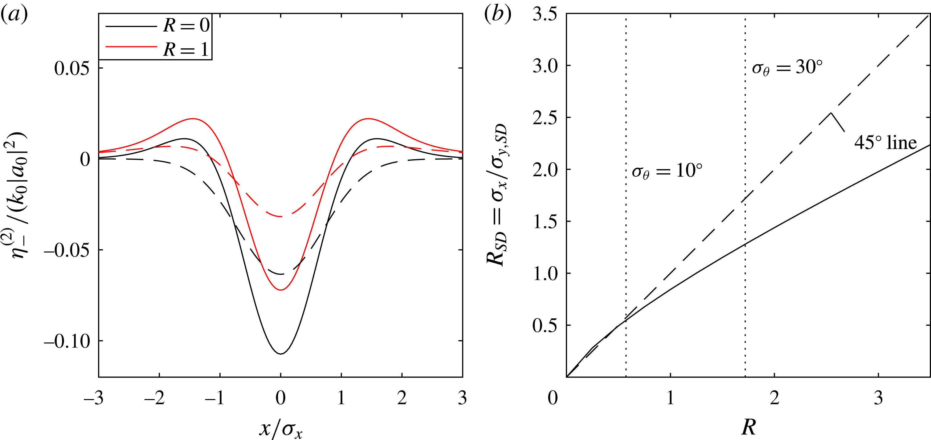
Figure 3. Theoretical aspects of the wave-averaged free surface for a single group: (a) set-down profile for a single wave group, showing the set-down for $d/\unicode[STIX]{x1D70E}_{x}=1.2=O(1)$
(continuous lines) and in the shallow return flow limit
$d/\unicode[STIX]{x1D70E}_{x}=1.2=O(1)$
(continuous lines) and in the shallow return flow limit $d/\unicode[STIX]{x1D70E}_{x}\rightarrow 0$
(dashed lines), and (b) aspect ratio of the wave-averaged free surface,
$d/\unicode[STIX]{x1D70E}_{x}\rightarrow 0$
(dashed lines), and (b) aspect ratio of the wave-averaged free surface, $R_{SD}$
, as a function of the aspect ratio of the group,
$R_{SD}$
, as a function of the aspect ratio of the group, $R\equiv \unicode[STIX]{x1D70E}_{x}/\unicode[STIX]{x1D70E}_{y}$
. We set
$R\equiv \unicode[STIX]{x1D70E}_{x}/\unicode[STIX]{x1D70E}_{y}$
. We set $\unicode[STIX]{x1D716}_{x}=0.30$
, corresponding to experiments.
$\unicode[STIX]{x1D716}_{x}=0.30$
, corresponding to experiments.
2.3 Two crossing groups: set-up and set-down
We now consider two quasimonochromatic wave groups that cross at $x=y=0$
(at
$x=y=0$
(at $t=0$
): group 1 with envelope
$t=0$
): group 1 with envelope $A_{1}$
travelling in the positive
$A_{1}$
travelling in the positive $x$
direction and group 2 with envelope
$x$
direction and group 2 with envelope $A_{2}$
travelling at an angle
$A_{2}$
travelling at an angle $\unicode[STIX]{x0394}\unicode[STIX]{x1D703}$
from group 1, with
$\unicode[STIX]{x0394}\unicode[STIX]{x1D703}$
from group 1, with $\unicode[STIX]{x0394}\unicode[STIX]{x1D703}$
measured anticlockwise from the positive
$\unicode[STIX]{x0394}\unicode[STIX]{x1D703}$
measured anticlockwise from the positive $x$
-axis. For simplicity, we assume that the two groups are entirely equivalent with the exception of their amplitudes and directions of travel, and have for the linear surface elevation
$x$
-axis. For simplicity, we assume that the two groups are entirely equivalent with the exception of their amplitudes and directions of travel, and have for the linear surface elevation
 $$\begin{eqnarray}\unicode[STIX]{x1D702}^{(1)}=Re[A_{1}(X_{1},Y_{1})\text{e}^{\text{i}(k_{0}x-\unicode[STIX]{x1D714}_{0}t)}+A_{2}(X_{2},Y_{2})\text{e}^{\text{i}(k_{0}x\cos (\unicode[STIX]{x0394}\unicode[STIX]{x1D703})+k_{0}y\sin (\unicode[STIX]{x0394}\unicode[STIX]{x1D703})-\unicode[STIX]{x1D714}_{0}t)}],\end{eqnarray}$$
where group 1 is a function of the slow scales $X_{1}=\unicode[STIX]{x1D716}_{x}(x-c_{g,0}t)$
and
$X_{1}=\unicode[STIX]{x1D716}_{x}(x-c_{g,0}t)$
and $Y_{1}=\unicode[STIX]{x1D716}_{y}y$
and group 2 of
$Y_{1}=\unicode[STIX]{x1D716}_{y}y$
and group 2 of $X_{2}=\unicode[STIX]{x1D716}_{x}(x\cos (\unicode[STIX]{x0394}\unicode[STIX]{x1D703})+y\sin (\unicode[STIX]{x0394}\unicode[STIX]{x1D703})-c_{g,0}t)$
and
$X_{2}=\unicode[STIX]{x1D716}_{x}(x\cos (\unicode[STIX]{x0394}\unicode[STIX]{x1D703})+y\sin (\unicode[STIX]{x0394}\unicode[STIX]{x1D703})-c_{g,0}t)$
and $Y_{2}=\unicode[STIX]{x1D716}_{y}(-x\sin (\unicode[STIX]{x0394}\unicode[STIX]{x1D703})+y\cos (\unicode[STIX]{x0394}\unicode[STIX]{x1D703}))$
, so that
$Y_{2}=\unicode[STIX]{x1D716}_{y}(-x\sin (\unicode[STIX]{x0394}\unicode[STIX]{x1D703})+y\cos (\unicode[STIX]{x0394}\unicode[STIX]{x1D703}))$
, so that $X_{1}$
and
$X_{1}$
and $X_{2}$
are in the direction of propagation of their respective groups. Substitution of (2.11) and its velocity potential counterpart
$X_{2}$
are in the direction of propagation of their respective groups. Substitution of (2.11) and its velocity potential counterpart $\unicode[STIX]{x1D719}^{(1)}$
into the mean flow forcing equation (2.3) gives after some manipulation and to leading-order in the multiple-scale parameter
$\unicode[STIX]{x1D719}^{(1)}$
into the mean flow forcing equation (2.3) gives after some manipulation and to leading-order in the multiple-scale parameter $\unicode[STIX]{x1D716}_{x}$
 $$\begin{eqnarray}\left.\frac{\unicode[STIX]{x2202}\unicode[STIX]{x1D719}_{-}^{(2)}}{\unicode[STIX]{x2202}z}\right|_{z=0}=\underbrace{F_{A1A1}+F_{A2A2}+F_{A1A2}}_{\equiv ~F},\end{eqnarray}$$
where the forcing is provided by the divergence of the Stokes transport of group 1 with envelope $A_{1}=|A_{1}|\exp (\text{i}\unicode[STIX]{x1D707}_{1})$
(
$A_{1}=|A_{1}|\exp (\text{i}\unicode[STIX]{x1D707}_{1})$
( $F_{A1A1}$
), group 2 with envelope
$F_{A1A1}$
), group 2 with envelope $A_{2}=|A_{1}|\exp (\text{i}\unicode[STIX]{x1D707}_{2})$
(
$A_{2}=|A_{1}|\exp (\text{i}\unicode[STIX]{x1D707}_{2})$
( $F_{A2A2}$
) and their interaction (
$F_{A2A2}$
) and their interaction ( $F_{A1A2}$
),
$F_{A1A2}$
),
 $$\begin{eqnarray}\left.\begin{array}{@{}rcl@{}}F_{A1A1}\ & =\ & \displaystyle {\textstyle \frac{1}{2}}\unicode[STIX]{x1D714}_{0}\unicode[STIX]{x1D716}_{x}\unicode[STIX]{x2202}_{X_{1}}|A_{1}|^{2},\\ F_{A2A2}\ & =\ & \displaystyle {\textstyle \frac{1}{2}}\unicode[STIX]{x1D714}_{0}\unicode[STIX]{x1D716}_{x}\unicode[STIX]{x2202}_{X_{2}}|A_{2}|^{2},\\ F_{A1A2}\ & =\ & \displaystyle \frac{1}{2}\unicode[STIX]{x1D714}_{0}\left(\frac{\unicode[STIX]{x1D716}_{x}(1+3\cos (\unicode[STIX]{x0394}\unicode[STIX]{x1D703}))}{2}(|A_{1}|_{X_{1}}|A_{2}|+|A_{1}||A_{2}|_{X_{2}})\right.\\ \ & \ & \left.+\,\unicode[STIX]{x1D716}_{y}\sin (\unicode[STIX]{x0394}\unicode[STIX]{x1D703})(|A_{1}|_{Y_{1}}|A_{2}|-|A_{1}||A_{2}|_{Y_{2}})\right)\\ \ & \ & \times \,\cos (k_{0}x(1-\cos (\unicode[STIX]{x0394}\unicode[STIX]{x1D703}))-k_{0}y\sin (\unicode[STIX]{x0394}\unicode[STIX]{x1D703})+\unicode[STIX]{x1D707}_{1}-\unicode[STIX]{x1D707}_{2}).\end{array}\right\}\end{eqnarray}$$
The phases of the two groups are denoted by $\unicode[STIX]{x1D707}_{1}$
and
$\unicode[STIX]{x1D707}_{1}$
and $\unicode[STIX]{x1D707}_{2}$
, and we have averaged over the fast temporal scales. The forcing and its response are no longer steady. Avoiding the prohibitively cumbersome Fourier transforms of
$\unicode[STIX]{x1D707}_{2}$
, and we have averaged over the fast temporal scales. The forcing and its response are no longer steady. Avoiding the prohibitively cumbersome Fourier transforms of $F_{A1A2}$
, we immediately assume that the return flow is shallow (
$F_{A1A2}$
, we immediately assume that the return flow is shallow ( $d/\unicode[STIX]{x1D70E}_{x}\ll 1$
), so that we can solve the two-dimensional Laplace equation subject to a distribution of sources and sinks of fluid given by (2.12)–(2.13) in physical space,
$d/\unicode[STIX]{x1D70E}_{x}\ll 1$
), so that we can solve the two-dimensional Laplace equation subject to a distribution of sources and sinks of fluid given by (2.12)–(2.13) in physical space,
 $$\begin{eqnarray}\unicode[STIX]{x1D719}_{-}^{(2)}(x,y,t)=-\frac{1}{4\unicode[STIX]{x03C0}d}\int _{-\infty }^{\infty }\int _{-\infty }^{\infty }F(x^{\ast },y^{\ast },t)\log ((x-x^{\ast })^{2}+(y-y^{\ast })^{2})\,\text{d}x^{\ast }\,\text{d}y^{\ast }.\end{eqnarray}$$
It can readily be shown that for $\unicode[STIX]{x0394}\unicode[STIX]{x1D703}=0$
, equation (2.14) reduces to the mean flow of a single group (2.7) with
$\unicode[STIX]{x0394}\unicode[STIX]{x1D703}=0$
, equation (2.14) reduces to the mean flow of a single group (2.7) with $A=A_{1}+A_{2}$
. Turning to its forcing equation (2.4), we decompose the wave-averaged surface elevation into a set-down
$A=A_{1}+A_{2}$
. Turning to its forcing equation (2.4), we decompose the wave-averaged surface elevation into a set-down $\unicode[STIX]{x1D702}_{SD}$
and an additional term, which we will later see arises because of wave crossing and we will term the crossing wave (CW) contribution
$\unicode[STIX]{x1D702}_{SD}$
and an additional term, which we will later see arises because of wave crossing and we will term the crossing wave (CW) contribution $\unicode[STIX]{x1D702}_{CW}$
,
$\unicode[STIX]{x1D702}_{CW}$
,
 $$\begin{eqnarray}\unicode[STIX]{x1D702}_{-}^{(2)}=\underbrace{\unicode[STIX]{x1D702}_{SD,A1A1}+\unicode[STIX]{x1D702}_{SD,A2A2}+\unicode[STIX]{x1D702}_{SD,A1A2}}_{=\unicode[STIX]{x1D702}_{SD}}+\unicode[STIX]{x1D702}_{CW}.\end{eqnarray}$$
The set-down arises purely in response to the return flow (i.e. through $-(1/g)\unicode[STIX]{x2202}\unicode[STIX]{x1D719}_{-}^{(2)}/\unicode[STIX]{x2202}t$
in (2.4)) and can be decomposed into three terms corresponding to the three forcing terms in (2.13). Corresponding to
$-(1/g)\unicode[STIX]{x2202}\unicode[STIX]{x1D719}_{-}^{(2)}/\unicode[STIX]{x2202}t$
in (2.4)) and can be decomposed into three terms corresponding to the three forcing terms in (2.13). Corresponding to $F_{A1A1}$
, we have after transforming into the reference frame of group 1
$F_{A1A1}$
, we have after transforming into the reference frame of group 1
 $$\begin{eqnarray}\unicode[STIX]{x1D702}_{SD,A1A1}(\tilde{x}_{1},{\tilde{y}}_{1})=\frac{|a_{1}|^{2}}{4d}\frac{1}{\unicode[STIX]{x03C0}\unicode[STIX]{x1D70E}_{x}^{2}}\int _{-\infty }^{\infty }\int _{-\infty }^{\infty }\frac{\text{e}^{-(\tilde{x}_{1}^{\ast })^{2}/\unicode[STIX]{x1D70E}_{x}^{2}-({\tilde{y}}_{1}^{\ast })^{2}/\unicode[STIX]{x1D70E}_{y}^{2}}\tilde{x}_{1}^{\ast }(\tilde{x}_{1}-\tilde{x}_{1}^{\ast })}{(\tilde{x}_{1}-\tilde{x}_{1}^{\ast })^{2}+({\tilde{y}}_{1}-{\tilde{y}}_{1}^{\ast })^{2}}\,\text{d}\tilde{x}_{1}^{\ast }\,\text{d}{\tilde{y}}_{1}^{\ast },\end{eqnarray}$$
where we have assumed a Gaussian envelope as before, namely $A_{1}=a_{1}\exp (-\tilde{x}_{1}^{2}/(2\unicode[STIX]{x1D70E}_{x}^{2})-{\tilde{y}}_{1}^{2}/(2\unicode[STIX]{x1D70E}_{y}^{2}))$
, with
$A_{1}=a_{1}\exp (-\tilde{x}_{1}^{2}/(2\unicode[STIX]{x1D70E}_{x}^{2})-{\tilde{y}}_{1}^{2}/(2\unicode[STIX]{x1D70E}_{y}^{2}))$
, with $a_{1}=|a_{1}|\exp (\text{i}\unicode[STIX]{x1D707}_{1})$
,
$a_{1}=|a_{1}|\exp (\text{i}\unicode[STIX]{x1D707}_{1})$
, $\tilde{x}_{1}=x-c_{g,0}t$
and
$\tilde{x}_{1}=x-c_{g,0}t$
and ${\tilde{y}}_{1}=y$
. By replacing (
${\tilde{y}}_{1}=y$
. By replacing ( $\tilde{x}_{1},{\tilde{y}}_{1}$
) with (
$\tilde{x}_{1},{\tilde{y}}_{1}$
) with ( $\tilde{x}_{2},{\tilde{y}}_{2}$
) and
$\tilde{x}_{2},{\tilde{y}}_{2}$
) and $|a_{1}|^{2}$
with
$|a_{1}|^{2}$
with $|a_{2}|^{2}$
, we can find an equivalent expression for the set-down
$|a_{2}|^{2}$
, we can find an equivalent expression for the set-down $\unicode[STIX]{x1D702}_{SD,A2A2}$
associated with group 2. Although the set-downs for the two individual groups are steady in their respective reference frames, their interaction is unsteady, and we have
$\unicode[STIX]{x1D702}_{SD,A2A2}$
associated with group 2. Although the set-downs for the two individual groups are steady in their respective reference frames, their interaction is unsteady, and we have
 $$\begin{eqnarray}\unicode[STIX]{x1D702}_{SD,A1A2}(\tilde{x},{\tilde{y}})=\frac{1}{4d}\frac{1}{\unicode[STIX]{x03C0}}\int _{-\infty }^{\infty }\int _{-\infty }^{\infty }\frac{1}{g}\frac{\unicode[STIX]{x2202}F_{A1A2}(x^{\ast },y^{\ast },t)}{\unicode[STIX]{x2202}t}\log ((x-x^{\ast })^{2}+(y-y^{\ast })^{2})\,\text{d}x^{\ast }\,\text{d}y^{\ast },\end{eqnarray}$$
where the forcing can be obtained by differentiating $F_{A1A2}$
in (2.13c
) with respect to time,
$F_{A1A2}$
in (2.13c
) with respect to time,
 $$\begin{eqnarray}\displaystyle \frac{1}{g}\frac{\unicode[STIX]{x2202}F_{A1A2}}{\unicode[STIX]{x2202}t} & = & \displaystyle -\frac{|A_{1}||A_{2}|}{4\unicode[STIX]{x1D70E}_{x}^{2}}\left(\frac{1+3\cos (\unicode[STIX]{x0394}\unicode[STIX]{x1D703})}{2}\left(\frac{(\tilde{x}_{1}+\tilde{x}_{2})^{2}}{\unicode[STIX]{x1D70E}_{x}^{2}}-2\right)\right.\nonumber\\ \displaystyle & & \displaystyle \left.+\,\sin (\unicode[STIX]{x0394}\unicode[STIX]{x1D703})\frac{(x\sin (\unicode[STIX]{x0394}\unicode[STIX]{x1D703})+y(1-\cos (\unicode[STIX]{x0394}\unicode[STIX]{x1D703})))(\tilde{x}_{1}+\tilde{x}_{2})}{\unicode[STIX]{x1D70E}_{y}^{2}}\right)\nonumber\\ \displaystyle & & \displaystyle \times \,\cos (k_{0}x(1-\cos (\unicode[STIX]{x0394}\unicode[STIX]{x1D703}))-k_{0}y\sin (\unicode[STIX]{x0394}\unicode[STIX]{x1D703})+\unicode[STIX]{x1D707}_{1}-\unicode[STIX]{x1D707}_{2}),\end{eqnarray}$$
where we use a mixture of coordinate systems for notational convenience. Apart from the set-down terms, the two terms on the right-hand side of (2.4) give rise to an additional term, after averaging over the fast temporal scales, which is responsible for the set-up, but is inherently associated with crossing waves,
 $$\begin{eqnarray}\displaystyle \unicode[STIX]{x1D702}_{CW} & = & \displaystyle \frac{-1}{g}\overline{\left(\left.\frac{\unicode[STIX]{x2202}^{2}\unicode[STIX]{x1D719}^{(1)}}{\unicode[STIX]{x2202}z\unicode[STIX]{x2202}t}\right|_{z=0}\unicode[STIX]{x1D702}^{(1)}+\left.\frac{1}{2}|\unicode[STIX]{x1D735}\unicode[STIX]{x1D719}|^{2}\right|_{z=0}\right)}\nonumber\\ \displaystyle & = & \displaystyle \frac{1}{2}(1-\cos (\unicode[STIX]{x0394}\unicode[STIX]{x1D703}))k_{0}|A_{1}||A_{2}|\nonumber\\ \displaystyle & & \displaystyle \times \,\cos (k_{0}(\underbrace{x(1-\cos (\unicode[STIX]{x0394}\unicode[STIX]{x1D703}))-y\sin (\unicode[STIX]{x0394}\unicode[STIX]{x1D703})}_{=\tilde{x}_{1}-\tilde{x}_{2}})+\unicode[STIX]{x1D707}_{1}-\unicode[STIX]{x1D707}_{2}).\end{eqnarray}$$
We note that, although the set-down is always slowly varying in both time and space, the crossing wave contribution (2.19) responsible for the set-up is slowly varying in time but rapidly varying in space. A partial standing-wave pattern forms with lines of constant phase at an angle $\unicode[STIX]{x0394}\unicode[STIX]{x1D703}/2$
to the
$\unicode[STIX]{x0394}\unicode[STIX]{x1D703}/2$
to the $x$
-axis, namely in line with the bisection of the paths of travel of the two groups. The pattern varies rapidly in space, and is slowly modulated in time and space by the product of the amplitude envelopes of the two groups (see figure 6
i–l). Whether
$x$
-axis, namely in line with the bisection of the paths of travel of the two groups. The pattern varies rapidly in space, and is slowly modulated in time and space by the product of the amplitude envelopes of the two groups (see figure 6
i–l). Whether $\unicode[STIX]{x1D702}_{CW}$
is actually manifested as a set-up of the wave-averaged free surface at the location of linear focus (
$\unicode[STIX]{x1D702}_{CW}$
is actually manifested as a set-up of the wave-averaged free surface at the location of linear focus ( $x=y=0$
) depends trivially on the relative phases of the two groups
$x=y=0$
) depends trivially on the relative phases of the two groups $(\unicode[STIX]{x1D707}_{1}-\unicode[STIX]{x1D707}_{2})$
. The presence of a set-up is thus an indicator of perfect or near-perfect focusing of the underlying linear signal (
$(\unicode[STIX]{x1D707}_{1}-\unicode[STIX]{x1D707}_{2})$
. The presence of a set-up is thus an indicator of perfect or near-perfect focusing of the underlying linear signal ( $\unicode[STIX]{x1D707}_{1}=\unicode[STIX]{x1D707}_{2}$
). It is noteworthy that (provided that
$\unicode[STIX]{x1D707}_{1}=\unicode[STIX]{x1D707}_{2}$
). It is noteworthy that (provided that $k_{0}d\gg 1$
) the magnitude of the wave crossing contribution is not a function of the magnitude of the depth relative to the scale of the group, unlike the set-down, which decreases in magnitude with increasing
$k_{0}d\gg 1$
) the magnitude of the wave crossing contribution is not a function of the magnitude of the depth relative to the scale of the group, unlike the set-down, which decreases in magnitude with increasing $d/\unicode[STIX]{x1D70E}_{x}$
. Finally, it is worth noting that the partial standing wave that forms the set-up does not have a counterpart in the second-order velocity field, unlike the set-down.
$d/\unicode[STIX]{x1D70E}_{x}$
. Finally, it is worth noting that the partial standing wave that forms the set-up does not have a counterpart in the second-order velocity field, unlike the set-down.
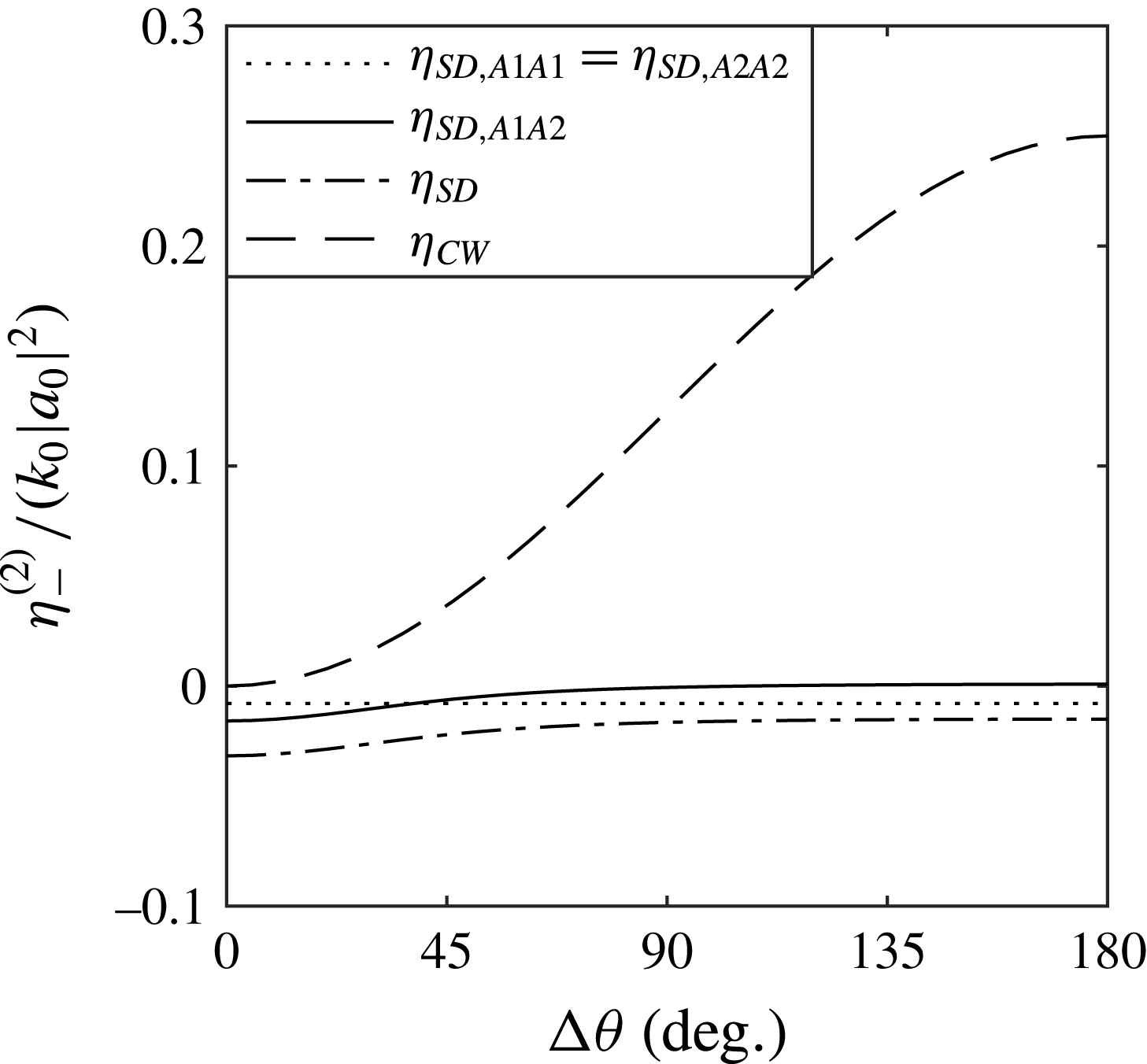
Figure 4. The different contributions to the total wave-averaged free surface at the focus point and time as a function of the crossing angle $\unicode[STIX]{x0394}\unicode[STIX]{x1D703}$
for two in-phase (
$\unicode[STIX]{x0394}\unicode[STIX]{x1D703}$
for two in-phase ( $\unicode[STIX]{x1D707}_{1}=\unicode[STIX]{x1D707}_{2}=0$
) round (
$\unicode[STIX]{x1D707}_{1}=\unicode[STIX]{x1D707}_{2}=0$
) round ( $R=1$
) wave groups (
$R=1$
) wave groups ( $\unicode[STIX]{x1D716}_{x}=0.30$
and
$\unicode[STIX]{x1D716}_{x}=0.30$
and $d/\unicode[STIX]{x1D70E}_{x}=1.2$
).
$d/\unicode[STIX]{x1D70E}_{x}=1.2$
).
In time, the behaviour of the wave-averaged free surface as the two groups cross is as follows: the groups are accompanied by a set-down before and after crossing; at the time of crossing, the wave-averaged free surface consists of a wave-group-like structure itself with a set-up at the focus location for the phases $\unicode[STIX]{x1D707}_{1}=\unicode[STIX]{x1D707}_{2}$
. Figure 4 shows the magnitudes of the different terms that compose the total wave-average surface in (2.15) as a function of
$\unicode[STIX]{x1D707}_{1}=\unicode[STIX]{x1D707}_{2}$
. Figure 4 shows the magnitudes of the different terms that compose the total wave-average surface in (2.15) as a function of $\unicode[STIX]{x0394}\unicode[STIX]{x1D703}$
. The self-interaction term
$\unicode[STIX]{x0394}\unicode[STIX]{x1D703}$
. The self-interaction term $\unicode[STIX]{x1D702}_{SD,A1A1}$
remains constant and negative, as it is independent of the interaction of the two groups, and similarly for
$\unicode[STIX]{x1D702}_{SD,A1A1}$
remains constant and negative, as it is independent of the interaction of the two groups, and similarly for $\unicode[STIX]{x1D702}_{SD,A2A2}$
. The cross-interaction set-down term
$\unicode[STIX]{x1D702}_{SD,A2A2}$
. The cross-interaction set-down term $\unicode[STIX]{x1D702}_{SD,A1A2}$
is initially negative and reduces to zero at
$\unicode[STIX]{x1D702}_{SD,A1A2}$
is initially negative and reduces to zero at $\unicode[STIX]{x0394}\unicode[STIX]{x1D703}=180^{\circ }$
. The set-down associated with two groups that collide head-on is simply equal to the sum of their respective set-downs,
$\unicode[STIX]{x0394}\unicode[STIX]{x1D703}=180^{\circ }$
. The set-down associated with two groups that collide head-on is simply equal to the sum of their respective set-downs, $\unicode[STIX]{x1D702}_{SD}=\unicode[STIX]{x1D702}_{SD,A1A1}+\unicode[STIX]{x1D702}_{SD,A2A2}$
. Finally, the crossing wave term
$\unicode[STIX]{x1D702}_{SD}=\unicode[STIX]{x1D702}_{SD,A1A1}+\unicode[STIX]{x1D702}_{SD,A2A2}$
. Finally, the crossing wave term $\unicode[STIX]{x1D702}_{CW}$
is zero for
$\unicode[STIX]{x1D702}_{CW}$
is zero for $\unicode[STIX]{x0394}\unicode[STIX]{x1D703}=0$
, as in this limit the solution reduces to that of a single group. For
$\unicode[STIX]{x0394}\unicode[STIX]{x1D703}=0$
, as in this limit the solution reduces to that of a single group. For $\unicode[STIX]{x0394}\unicode[STIX]{x1D703}\rightarrow 180^{\circ }$
, the crossing wave term increases to a maximum, as can also be readily concluded from inspection of (2.19).
$\unicode[STIX]{x0394}\unicode[STIX]{x1D703}\rightarrow 180^{\circ }$
, the crossing wave term increases to a maximum, as can also be readily concluded from inspection of (2.19).
Summarizing results, the behaviour of the wave-averaged free surface is driven by two distinct physical processes, the first of which can only give rise to a set-down and the second of which takes the form of a modulated partial standing-wave pattern and may or may not give rise to a set-up. The set-down forms as the simple free-surface manifestation of the Eulerian return flow that forms underneath a group in response to the divergence of the Stokes transport on the group scale. The set-down can be computed directly from the unsteady Bernoulli equation, retaining the unsteady potential corresponding to the return flow (and ignoring all other terms). The magnitude of the set-down reduces with increasing directional spreading, as the return flow can flow around as well as underneath the group and reduces in magnitude. The set-down does not form for periodic waves; it depends on the group structure. Although its magnitude does not depend on the group width in the limit in which the group width is larger relative to the water depth, it generally reduces with increasing group width. When two groups (or indeed two periodic waves) cross at an angle, further terms in the Bernoulli equation, which are zero for deep water and for a single group or a crossing angle of zero degrees, give rise to a partial standing-wave pattern. Its magnitude does not depend on the group width or on the water depth, provided that $k_{0}d\gg 1$
. The standing-wave pattern is fixed in space and is modulated by the product of the two groups in both space and time. A set-up forms at the point of focus and crossing, if the two groups are in phase, so that their amplitudes are both positive there.
$k_{0}d\gg 1$
. The standing-wave pattern is fixed in space and is modulated by the product of the two groups in both space and time. A set-up forms at the point of focus and crossing, if the two groups are in phase, so that their amplitudes are both positive there.
2.4 Multicomponent second-order theory (review)
The expressions for the wave-averaged free-surface elevation derived thus far have relied on two approximations: the spectrum is narrow-banded in both frequency and direction, so that the group can be modelled using the leading-order terms in a multiple-scale expansion. By considering the linear signal as the sum of individual components with different frequencies travelling in different directions, Hasselmann (Reference Hasselmann1962) implicitly and, much later yet explicitly, Sharma & Dean (Reference Sharma and Dean1981), Dalzell (Reference Dalzell1999) and Forristall (Reference Forristall2000) derived interaction kernels for the nonlinear bound harmonics at second order. We assume independence between the directional $\unicode[STIX]{x1D6FA}$
and amplitude
$\unicode[STIX]{x1D6FA}$
and amplitude $\hat{\unicode[STIX]{x1D702}}$
distributions, so that the linear signal is given by a summation over
$\hat{\unicode[STIX]{x1D702}}$
distributions, so that the linear signal is given by a summation over $N_{k}$
discrete components in
$N_{k}$
discrete components in $N_{\unicode[STIX]{x1D703}}$
directions,
$N_{\unicode[STIX]{x1D703}}$
directions,
 $$\begin{eqnarray}\unicode[STIX]{x1D702}^{(1)}=\mathop{\sum }_{n=1}^{N_{k}}\mathop{\sum }_{i=1}^{N_{\unicode[STIX]{x1D703}}}\unicode[STIX]{x1D6FA}(\unicode[STIX]{x1D703}_{i})\hat{\unicode[STIX]{x1D702}}_{n}\cos (\unicode[STIX]{x1D711}_{n,i})\unicode[STIX]{x1D6FF}k\unicode[STIX]{x1D6FF}\unicode[STIX]{x1D703},\quad \text{with }\unicode[STIX]{x1D711}_{n,i}=\boldsymbol{k}_{n,i}\boldsymbol{\cdot }\boldsymbol{x}-\unicode[STIX]{x1D714}_{n}t+\unicode[STIX]{x1D707}_{n},\end{eqnarray}$$
where the wavenumber vector $\boldsymbol{k}_{n,i}=k_{n}(\cos (\unicode[STIX]{x1D703}_{i}),\sin (\unicode[STIX]{x1D703}_{i}))$
has magnitude
$\boldsymbol{k}_{n,i}=k_{n}(\cos (\unicode[STIX]{x1D703}_{i}),\sin (\unicode[STIX]{x1D703}_{i}))$
has magnitude $k_{n}$
and
$k_{n}$
and $\unicode[STIX]{x1D703}$
is measured anticlockwise from the positive
$\unicode[STIX]{x1D703}$
is measured anticlockwise from the positive $x$
-axis. Every component satisfies the linear dispersion relationship
$x$
-axis. Every component satisfies the linear dispersion relationship $\unicode[STIX]{x1D714}_{n}^{2}=gk_{n}\tanh (k_{n}d)$
, where
$\unicode[STIX]{x1D714}_{n}^{2}=gk_{n}\tanh (k_{n}d)$
, where $\tanh (kd)\approx 1$
for almost all components of the linear spectrum in our experiments. The coefficients
$\tanh (kd)\approx 1$
for almost all components of the linear spectrum in our experiments. The coefficients $\unicode[STIX]{x1D6FF}k$
and
$\unicode[STIX]{x1D6FF}k$
and $\unicode[STIX]{x1D6FF}\unicode[STIX]{x1D703}$
correspond to the magnitude of the discrete steps, so that
$\unicode[STIX]{x1D6FF}\unicode[STIX]{x1D703}$
correspond to the magnitude of the discrete steps, so that $\unicode[STIX]{x1D6FF}k\rightarrow \text{d}k$
as
$\unicode[STIX]{x1D6FF}k\rightarrow \text{d}k$
as $N_{k}\rightarrow \infty$
and similarly for
$N_{k}\rightarrow \infty$
and similarly for $\unicode[STIX]{x1D6FF}\unicode[STIX]{x1D703}$
. The corresponding second-order difference waves that represent the wave-averaged free surface may be calculated as (Dalzell Reference Dalzell1999)
$\unicode[STIX]{x1D6FF}\unicode[STIX]{x1D703}$
. The corresponding second-order difference waves that represent the wave-averaged free surface may be calculated as (Dalzell Reference Dalzell1999)
 $$\begin{eqnarray}\unicode[STIX]{x1D702}_{-}^{(2)}=\mathop{\sum }_{n=1}^{N_{k}}\mathop{\sum }_{m=1}^{N_{k}}\mathop{\sum }_{i=1}^{N_{\unicode[STIX]{x1D703}}}\mathop{\sum }_{j=1}^{N_{\unicode[STIX]{x1D703}}}\unicode[STIX]{x1D6FA}(\unicode[STIX]{x1D703}_{i})\unicode[STIX]{x1D6FA}(\unicode[STIX]{x1D703}_{j})\hat{\unicode[STIX]{x1D702}}_{n}\hat{\unicode[STIX]{x1D702}}_{m}B^{-}(\boldsymbol{k}_{n,i},\boldsymbol{k}_{m,j},\unicode[STIX]{x1D714}_{n},\unicode[STIX]{x1D714}_{m},d)\cos (\unicode[STIX]{x1D711}_{n,i}-\unicode[STIX]{x1D711}_{m,j})(\unicode[STIX]{x1D6FF}k)^{2}(\unicode[STIX]{x1D6FF}\unicode[STIX]{x1D703})^{2},\end{eqnarray}$$
where the interaction kernel $B^{-}$
is given in appendix A.
$B^{-}$
is given in appendix A.

Figure 5. Contours of the wave-averaged surface elevation $\unicode[STIX]{x1D702}_{-}^{(2)}$
for a single group at time of linear focus for different degrees of spreading
$\unicode[STIX]{x1D702}_{-}^{(2)}$
for a single group at time of linear focus for different degrees of spreading $\unicode[STIX]{x1D70E}_{\unicode[STIX]{x1D703}}$
; (a–d) are computed from multicomponent second-order theory (2.21) and (e–h) correspond to the quasimonochromatic limit (2.8), as denoted by
$\unicode[STIX]{x1D70E}_{\unicode[STIX]{x1D703}}$
; (a–d) are computed from multicomponent second-order theory (2.21) and (e–h) correspond to the quasimonochromatic limit (2.8), as denoted by $\unicode[STIX]{x1D716}_{x}\rightarrow 0$
. The aspect ratio in the quasimonochromatic limit is computed from
$\unicode[STIX]{x1D716}_{x}\rightarrow 0$
. The aspect ratio in the quasimonochromatic limit is computed from $R=\unicode[STIX]{x1D70E}_{\unicode[STIX]{x1D703}}/\unicode[STIX]{x1D716}_{x}$
, which is asymptotically valid in the limit of a small degree of spreading (
$R=\unicode[STIX]{x1D70E}_{\unicode[STIX]{x1D703}}/\unicode[STIX]{x1D716}_{x}$
, which is asymptotically valid in the limit of a small degree of spreading ( $R=0.6$
,
$R=0.6$
, $1.1$
,
$1.1$
, $1.7$
,
$1.7$
, $2.3$
for the four values of
$2.3$
for the four values of $\unicode[STIX]{x1D70E}_{\unicode[STIX]{x1D703}}$
respectively). The black dashed lines correspond to two standard deviations from the centre of the group.
$\unicode[STIX]{x1D70E}_{\unicode[STIX]{x1D703}}$
respectively). The black dashed lines correspond to two standard deviations from the centre of the group.
For the experimental parameters considered herein ( $\unicode[STIX]{x1D6FC}=k_{0}a_{0}=0.20$
,
$\unicode[STIX]{x1D6FC}=k_{0}a_{0}=0.20$
, $\unicode[STIX]{x1D716}_{x}=1/(k_{0}\unicode[STIX]{x1D70E}_{x})=0.30$
,
$\unicode[STIX]{x1D716}_{x}=1/(k_{0}\unicode[STIX]{x1D70E}_{x})=0.30$
, $k_{0}d=3.9$
and
$k_{0}d=3.9$
and $d/\unicode[STIX]{x1D70E}_{x}=1.2$
), discussed in more detail in § 3, figure 5 compares the component-by-component solution (2.21) (a–d) with the multiple-scale solution for the set-down (2.8) (e–h) for a single wave group, demonstrating good agreement for low degrees of spreading. The mean direction of wave group propagation is left to right in the positive
$d/\unicode[STIX]{x1D70E}_{x}=1.2$
), discussed in more detail in § 3, figure 5 compares the component-by-component solution (2.21) (a–d) with the multiple-scale solution for the set-down (2.8) (e–h) for a single wave group, demonstrating good agreement for low degrees of spreading. The mean direction of wave group propagation is left to right in the positive $x$
direction. For high degrees of spreading, a set-up starts to appear in the form of a ridge along the
$x$
direction. For high degrees of spreading, a set-up starts to appear in the form of a ridge along the $x$
-axis that connects the humps in front of and behind the group and that is not predicted by the multiple-scale solution (2.8).
$x$
-axis that connects the humps in front of and behind the group and that is not predicted by the multiple-scale solution (2.8).
Figure 6 compares the component-by-component solution (2.21) (a–d) for two crossing groups at four different crossing angles with the multiple-scale solution (2.15) (m–p). Also shown are the individual contributions from the set-down (2.16)–(2.17) in (e)–(h) and the crossing wave pattern (2.19) in (i)–(l). It is evident from this comparison that the multiple-scale solution can predict the magnitude, but not the exact spatial structure, of the set-down for $\unicode[STIX]{x0394}\unicode[STIX]{x1D703}=45^{\circ }$
, as the directional spectra of the group are not clearly separated for low crossing angles. For all larger crossing angles, the two methods agree well, and the set-up is dominant.
$\unicode[STIX]{x0394}\unicode[STIX]{x1D703}=45^{\circ }$
, as the directional spectra of the group are not clearly separated for low crossing angles. For all larger crossing angles, the two methods agree well, and the set-up is dominant.

Figure 6. Contours of the wave-averaged surface elevation $\unicode[STIX]{x1D702}_{-}^{(2)}$
for crossing wave groups at time of linear focus for different crossing angles
$\unicode[STIX]{x1D702}_{-}^{(2)}$
for crossing wave groups at time of linear focus for different crossing angles $\unicode[STIX]{x0394}\unicode[STIX]{x1D703}$
; (a–d) are computed from multicomponent second-order theory (2.21), (e–h) correspond to the set-down in the quasimonochromatic limit (2.16)–(2.17), (i–l) correspond to the crossing wave pattern in the quasimonochromatic limit (2.19) and (m–p) correspond to the sum of the last two. The degree of spreading of the individual groups is
$\unicode[STIX]{x0394}\unicode[STIX]{x1D703}$
; (a–d) are computed from multicomponent second-order theory (2.21), (e–h) correspond to the set-down in the quasimonochromatic limit (2.16)–(2.17), (i–l) correspond to the crossing wave pattern in the quasimonochromatic limit (2.19) and (m–p) correspond to the sum of the last two. The degree of spreading of the individual groups is $\unicode[STIX]{x1D70E}_{\unicode[STIX]{x1D703}}=10^{\circ }$
.
$\unicode[STIX]{x1D70E}_{\unicode[STIX]{x1D703}}=10^{\circ }$
.
3 Experimental method
This section introduces the experimental set-up (§ 3.1), details the input parameters of each category of experiment (§ 3.2) and introduces the method used to isolate the wave-averaged surface elevation from the measured signal (§ 3.3). Sections 3.4 and 3.5 respectively describe our estimation of spectral and directional parameters from the measured signal. Finally, § 3.6 discusses sources of measurement error and repeatability.
3.1 FloWave and gauge layout
The experiments are conducted at the FloWave Ocean Energy Research Facility at the University of Edinburgh. The circular multidirectional wave basin has a $25~\text{m}$
diameter, is
$25~\text{m}$
diameter, is $2~\text{m}$
deep and is encircled by 168 actively absorbing force-feedback wavemakers, allowing for the creation of waves in all directions. All of our experiments are of sufficiently short duration, with a run time of 32 s, for reflections not to play a role. The generation of waves by the wavemakers is based on linear theory.
$2~\text{m}$
deep and is encircled by 168 actively absorbing force-feedback wavemakers, allowing for the creation of waves in all directions. All of our experiments are of sufficiently short duration, with a run time of 32 s, for reflections not to play a role. The generation of waves by the wavemakers is based on linear theory.
Figure 7 shows the layout of the array, consisting of 14 capacitance wave gauges within the tank, with gauge locations chosen to combine good spatial resolution while being spaced far enough apart to capture the entire spatial structure of the wave-averaged free surface. Practically constrained by a limited number of wave gauges available and their robust positioning on an overhanging gantry, we place all of our wave gauges along the main axis of travel of the group ( $x$
-axis) and on the positive half of the orthogonal
$x$
-axis) and on the positive half of the orthogonal $y$
-axis (with the exception of one further gauge at negative
$y$
-axis (with the exception of one further gauge at negative $y$
), as illustrated by the closed circles in figure 7. To gain additional information on the two-dimensional structure of the free surface, we repeat (a selection of) the same experiments varying their angle of propagation relative to the gauge array, thus obtaining the effective gauge layout illustrated by the open circles in figure 7. These repetitions are carried out at intervals of
$y$
), as illustrated by the closed circles in figure 7. To gain additional information on the two-dimensional structure of the free surface, we repeat (a selection of) the same experiments varying their angle of propagation relative to the gauge array, thus obtaining the effective gauge layout illustrated by the open circles in figure 7. These repetitions are carried out at intervals of $22.5^{\circ }$
between
$22.5^{\circ }$
between $0^{\circ }$
and
$0^{\circ }$
and $90^{\circ }$
, as illustrated by the arrows in figure 7(a). The wave gauges are calibrated at the start of each day of testing. A settling time of 10 min between each test is employed to allow for the absorption of reflected waves.
$90^{\circ }$
, as illustrated by the arrows in figure 7(a). The wave gauges are calibrated at the start of each day of testing. A settling time of 10 min between each test is employed to allow for the absorption of reflected waves.

Figure 7. The gauge array layout, showing wave gauge locations with respect to the centre of the tank ( $x=0$
,
$x=0$
, $y=0$
). The closed circles denote the location of the 14 gauges with the positive
$y=0$
). The closed circles denote the location of the 14 gauges with the positive $x$
-axis corresponding to the mean direction of travel of the group (or one of the groups). The open circles denote the effective gauge layout achieved by changing the mean wave direction in steps of
$x$
-axis corresponding to the mean direction of travel of the group (or one of the groups). The open circles denote the effective gauge layout achieved by changing the mean wave direction in steps of $22.5^{\circ }$
to map out the wave-averaged free surface. The arrows in (a) illustrate the mean direction of each repeated test used to achieve this.
$22.5^{\circ }$
to map out the wave-averaged free surface. The arrows in (a) illustrate the mean direction of each repeated test used to achieve this.
Table 1. Matrix of experiments.
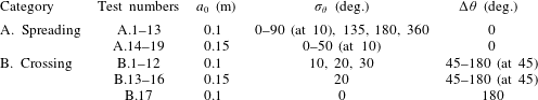
3.2 Matrix of experiments and input parameters
We conduct tests in two categories: spreading tests (category A, § 3.2.1) and crossing tests (category B, § 3.2.2), as summarized in table 1. In these two categories of test, we respectively vary the degree of directional spreading for a single group (A) and consider two crossing groups for different crossing angles (B). For all experiments, we base the input on a Gaussian amplitude distribution in wavenumber magnitude $k=|\boldsymbol{k}|$
,
$k=|\boldsymbol{k}|$
,
 $$\begin{eqnarray}\hat{\unicode[STIX]{x1D702}}(k)=\frac{a_{0}}{\sqrt{2\unicode[STIX]{x03C0}}\unicode[STIX]{x0394}k}\exp \left(-\frac{1}{2}\left(\frac{k-k_{0}}{\unicode[STIX]{x0394}k}\right)^{2}\right)\quad \text{for }0\leqslant k\leqslant \infty ,\end{eqnarray}$$
which is converted into the frequency domain using the linear dispersion relationship before being provided as an input to the wavemakers. We set the peak wavenumber $k_{0}=2.0~\text{m}^{-1}$
(based on a peak frequency of 0.7 Hz) and adopt a standard deviation of
$k_{0}=2.0~\text{m}^{-1}$
(based on a peak frequency of 0.7 Hz) and adopt a standard deviation of $\unicode[STIX]{x0394}k=0.6~\text{m}^{-1}$
. Although (3.1) only formally corresponds to a group with a Gaussian envelope in real space if
$\unicode[STIX]{x0394}k=0.6~\text{m}^{-1}$
. Although (3.1) only formally corresponds to a group with a Gaussian envelope in real space if $k$
has support on the entire real line (including
$k$
has support on the entire real line (including $k<0$
),
$k<0$
), $S(k)$
is negligibly small for
$S(k)$
is negligibly small for $k=0$
and below for the parameters chosen. Thus,
$k=0$
and below for the parameters chosen. Thus, $\unicode[STIX]{x1D70E}_{x}=1/\unicode[STIX]{x0394}k=1.7~\text{m}$
corresponds to the spatial scale of the group (the standard deviation of the approximately Gaussian group). We have
$\unicode[STIX]{x1D70E}_{x}=1/\unicode[STIX]{x0394}k=1.7~\text{m}$
corresponds to the spatial scale of the group (the standard deviation of the approximately Gaussian group). We have $\unicode[STIX]{x1D716}_{x}=0.30$
, so the multiple-scale approximation will probably hold, but be associated with an error that scales as
$\unicode[STIX]{x1D716}_{x}=0.30$
, so the multiple-scale approximation will probably hold, but be associated with an error that scales as $\unicode[STIX]{x1D716}_{x}^{2}\;({\sim}10\,\%)$
. We choose this large value of
$\unicode[STIX]{x1D716}_{x}^{2}\;({\sim}10\,\%)$
. We choose this large value of $\unicode[STIX]{x1D716}_{x}$
so that the spatial extent of the group is considerably smaller than that of the tank. This ensures that long second-order error waves associated with the linear paddle motion have time to propagate ahead of the group. Our linear wave is always deep
$\unicode[STIX]{x1D716}_{x}$
so that the spatial extent of the group is considerably smaller than that of the tank. This ensures that long second-order error waves associated with the linear paddle motion have time to propagate ahead of the group. Our linear wave is always deep $(k_{0}d=3.9)$
and we choose the total linear amplitude
$(k_{0}d=3.9)$
and we choose the total linear amplitude $a_{0}$
to be 0.1 or 0.15 m, corresponding to a steepness of
$a_{0}$
to be 0.1 or 0.15 m, corresponding to a steepness of $\unicode[STIX]{x1D6FC}=k_{0}a_{0}=0.20$
or
$\unicode[STIX]{x1D6FC}=k_{0}a_{0}=0.20$
or $0.30$
. The steepness of the wave groups is chosen to produce second-order components sufficiently large to observe, while minimizing the effects of higher-order nonlinearity. Wave breaking is not observed during the experiments and is not expected for individual (directionally spread) short groups of such steepness. We consider a Gaussian amplitude distribution in angle
$0.30$
. The steepness of the wave groups is chosen to produce second-order components sufficiently large to observe, while minimizing the effects of higher-order nonlinearity. Wave breaking is not observed during the experiments and is not expected for individual (directionally spread) short groups of such steepness. We consider a Gaussian amplitude distribution in angle $\unicode[STIX]{x1D703}$
,
$\unicode[STIX]{x1D703}$
,
 $$\begin{eqnarray}\unicode[STIX]{x1D6FA}(\unicode[STIX]{x1D703})=\frac{\unicode[STIX]{x1D6FA}_{0}}{\sqrt{2\unicode[STIX]{x03C0}}\unicode[STIX]{x1D70E}_{\unicode[STIX]{x1D703}}}\exp \left(-\frac{1}{2}\left(\frac{\unicode[STIX]{x1D703}-\unicode[STIX]{x1D703}_{0}}{\unicode[STIX]{x1D70E}_{\unicode[STIX]{x1D703}}}\right)^{2}\right)\quad \text{for }-180^{\circ }\leqslant \unicode[STIX]{x1D703}\leqslant 180^{\circ },\end{eqnarray}$$
where $\unicode[STIX]{x1D703}_{0}$
is the mean direction and
$\unicode[STIX]{x1D703}_{0}$
is the mean direction and $\unicode[STIX]{x1D70E}_{\unicode[STIX]{x1D703}}$
is a measure of the degree of directional spreading. We truncate the spreading distribution at
$\unicode[STIX]{x1D70E}_{\unicode[STIX]{x1D703}}$
is a measure of the degree of directional spreading. We truncate the spreading distribution at $-180^{\circ }$
and
$-180^{\circ }$
and $+180^{\circ }$
and choose the normalization coefficient
$+180^{\circ }$
and choose the normalization coefficient $\unicode[STIX]{x1D6FA}_{0}$
so that the sum of
$\unicode[STIX]{x1D6FA}_{0}$
so that the sum of $\unicode[STIX]{x1D6FA}(\unicode[STIX]{x1D703})$
is unity over this range. For small degrees of spreading,
$\unicode[STIX]{x1D6FA}(\unicode[STIX]{x1D703})$
is unity over this range. For small degrees of spreading, $\unicode[STIX]{x1D70E}_{\unicode[STIX]{x1D703}}$
corresponds to the root-mean-squared spreading value. For crossing wave groups, two directional distribution functions with different values of
$\unicode[STIX]{x1D70E}_{\unicode[STIX]{x1D703}}$
corresponds to the root-mean-squared spreading value. For crossing wave groups, two directional distribution functions with different values of $\unicode[STIX]{x1D703}_{0}$
are superimposed. We emphasize the difference between our
$\unicode[STIX]{x1D703}_{0}$
are superimposed. We emphasize the difference between our $\unicode[STIX]{x1D70E}_{\unicode[STIX]{x1D703}}$
and the usual energy spectrum directional spreading parameter, which is equal to
$\unicode[STIX]{x1D70E}_{\unicode[STIX]{x1D703}}$
and the usual energy spectrum directional spreading parameter, which is equal to $\unicode[STIX]{x1D70E}_{\unicode[STIX]{x1D703}}/\sqrt{2}$
.
$\unicode[STIX]{x1D70E}_{\unicode[STIX]{x1D703}}/\sqrt{2}$
.
3.2.1 Category A – spreading tests
First, tests are carried out to assess the relationship between the degree of directional spreading $\unicode[STIX]{x1D70E}_{\unicode[STIX]{x1D703}}$
, and the amplitude and sign of the wave-averaged surface elevation for a single focused wave group. The degree of directional spreading
$\unicode[STIX]{x1D70E}_{\unicode[STIX]{x1D703}}$
, and the amplitude and sign of the wave-averaged surface elevation for a single focused wave group. The degree of directional spreading $\unicode[STIX]{x1D70E}_{\unicode[STIX]{x1D703}}$
is varied in the range
$\unicode[STIX]{x1D70E}_{\unicode[STIX]{x1D703}}$
is varied in the range $0{-}360^{\circ }$
for groups with an amplitude of
$0{-}360^{\circ }$
for groups with an amplitude of $a_{0}=0.1~\text{m}$
, and in the range
$a_{0}=0.1~\text{m}$
, and in the range $\unicode[STIX]{x1D70E}_{\unicode[STIX]{x1D703}}=0{-}50^{\circ }$
for an increased amplitude of
$\unicode[STIX]{x1D70E}_{\unicode[STIX]{x1D703}}=0{-}50^{\circ }$
for an increased amplitude of $a_{0}=0.15~\text{m}$
. In practice,
$a_{0}=0.15~\text{m}$
. In practice, $\unicode[STIX]{x1D70E}_{\unicode[STIX]{x1D703}}=360^{\circ }$
corresponds to the case where the directional spectrum has almost fully saturated (
$\unicode[STIX]{x1D70E}_{\unicode[STIX]{x1D703}}=360^{\circ }$
corresponds to the case where the directional spectrum has almost fully saturated ( $\unicode[STIX]{x1D70E}_{\unicode[STIX]{x1D703}}\rightarrow \infty$
corresponds to fully axisymmetric spreading: the variation of
$\unicode[STIX]{x1D70E}_{\unicode[STIX]{x1D703}}\rightarrow \infty$
corresponds to fully axisymmetric spreading: the variation of $\unicode[STIX]{x1D6FA}(\unicode[STIX]{x1D703})$
as a function of
$\unicode[STIX]{x1D6FA}(\unicode[STIX]{x1D703})$
as a function of $\unicode[STIX]{x1D703}$
is less than 7 % for
$\unicode[STIX]{x1D703}$
is less than 7 % for $\unicode[STIX]{x1D70E}_{\unicode[STIX]{x1D703}}=360^{\circ }$
). The difference in the amplitude of the wave-averaged surface elevation between
$\unicode[STIX]{x1D70E}_{\unicode[STIX]{x1D703}}=360^{\circ }$
). The difference in the amplitude of the wave-averaged surface elevation between $\unicode[STIX]{x1D70E}_{\unicode[STIX]{x1D703}}=360^{\circ }$
and
$\unicode[STIX]{x1D70E}_{\unicode[STIX]{x1D703}}=360^{\circ }$
and $\unicode[STIX]{x1D70E}_{\unicode[STIX]{x1D703}}\rightarrow \infty$
is negligible (
$\unicode[STIX]{x1D70E}_{\unicode[STIX]{x1D703}}\rightarrow \infty$
is negligible ( ${<}0.1\,\%$
). An illustration of three of these tests is presented in figure 1 for
${<}0.1\,\%$
). An illustration of three of these tests is presented in figure 1 for $\unicode[STIX]{x1D70E}_{\unicode[STIX]{x1D703}}=10$
,
$\unicode[STIX]{x1D70E}_{\unicode[STIX]{x1D703}}=10$
, $20$
,
$20$
, $30^{\circ }$
.
$30^{\circ }$
.
Having observed the temporal behaviour of the wave-averaged surface elevation of directionally spread wave groups at the point of intended linear focus, we seek to gain further understanding by measuring the spatial variation of the wave-averaged surface elevation. We achieve this by repeating certain tests and varying the mean direction of propagation relative to the gauge array from $0$
to
$0$
to $90^{\circ }$
and at intervals of
$90^{\circ }$
and at intervals of $22.5^{\circ }$
. In doing so, we capture the spatial structure of the wave-averaged surface elevation, as measured with the effective gauge layout shown by the open circles in figure 7. We map the wave-averaged free surface by carrying out such repeats for four tests from this category,
$22.5^{\circ }$
. In doing so, we capture the spatial structure of the wave-averaged surface elevation, as measured with the effective gauge layout shown by the open circles in figure 7. We map the wave-averaged free surface by carrying out such repeats for four tests from this category, $\unicode[STIX]{x1D70E}_{\unicode[STIX]{x1D703}}=20,30,40^{\circ }$
(and at an increased amplitude of
$\unicode[STIX]{x1D70E}_{\unicode[STIX]{x1D703}}=20,30,40^{\circ }$
(and at an increased amplitude of $a_{0}=0.15~\text{m}$
for
$a_{0}=0.15~\text{m}$
for $\unicode[STIX]{x1D70E}_{\unicode[STIX]{x1D703}}=40^{\circ }$
). In doing so, we capture the spatial structure of the wave-averaged free surface dominated by the set-down, the set-up and the transition between these as a function of
$\unicode[STIX]{x1D70E}_{\unicode[STIX]{x1D703}}=40^{\circ }$
). In doing so, we capture the spatial structure of the wave-averaged free surface dominated by the set-down, the set-up and the transition between these as a function of $\unicode[STIX]{x1D70E}_{\unicode[STIX]{x1D703}}$
.
$\unicode[STIX]{x1D70E}_{\unicode[STIX]{x1D703}}$
.
3.2.2 Category B – crossing tests
Second, tests are carried out to assess the relationship between the crossing angle $\unicode[STIX]{x0394}\unicode[STIX]{x1D703}$
of two directionally spread focused wave groups and the set-up or set-down of the wave-averaged surface elevation. The crossing angle
$\unicode[STIX]{x0394}\unicode[STIX]{x1D703}$
of two directionally spread focused wave groups and the set-up or set-down of the wave-averaged surface elevation. The crossing angle $\unicode[STIX]{x0394}\unicode[STIX]{x1D703}$
of the wave groups is varied between
$\unicode[STIX]{x0394}\unicode[STIX]{x1D703}$
of the wave groups is varied between $0$
and
$0$
and $180^{\circ }$
at
$180^{\circ }$
at $45^{\circ }$
intervals. This is repeated for groups with directional spreading of
$45^{\circ }$
intervals. This is repeated for groups with directional spreading of $\unicode[STIX]{x1D70E}_{\unicode[STIX]{x1D703}}=10,20,30^{\circ }$
and
$\unicode[STIX]{x1D70E}_{\unicode[STIX]{x1D703}}=10,20,30^{\circ }$
and $a_{0}=0.1~\text{m}$
(and for an increased amplitude of
$a_{0}=0.1~\text{m}$
(and for an increased amplitude of $a_{0}=0.15~\text{m}$
at
$a_{0}=0.15~\text{m}$
at $\unicode[STIX]{x1D70E}_{\unicode[STIX]{x1D703}}=20^{\circ }$
). An illustration of one of these tests is presented in figure 2 for
$\unicode[STIX]{x1D70E}_{\unicode[STIX]{x1D703}}=20^{\circ }$
). An illustration of one of these tests is presented in figure 2 for $\unicode[STIX]{x1D70E}_{\unicode[STIX]{x1D703}}=10^{\circ }$
and
$\unicode[STIX]{x1D70E}_{\unicode[STIX]{x1D703}}=10^{\circ }$
and $\unicode[STIX]{x0394}\unicode[STIX]{x1D703}=135^{\circ }$
.
$\unicode[STIX]{x0394}\unicode[STIX]{x1D703}=135^{\circ }$
.
3.3 Harmonic separation
In order to observe the wave-averaged free surface of wave groups and other nonlinear harmonics, these components must be extracted from the fully nonlinear signal measured by the gauges. By repeating experiments and changing the phases of all of the linear components of the wave group in the wavemaker signal by $180^{\circ }$
between experiments, nonlinear harmonic terms of odd and even powers in amplitude may be extracted from the measured time series (Baldock, Swan & Taylor Reference Baldock, Swan and Taylor1996),
$180^{\circ }$
between experiments, nonlinear harmonic terms of odd and even powers in amplitude may be extracted from the measured time series (Baldock, Swan & Taylor Reference Baldock, Swan and Taylor1996),
 $$\begin{eqnarray}\unicode[STIX]{x1D702}_{odd}=\frac{\unicode[STIX]{x1D702}_{0}-\unicode[STIX]{x1D702}_{180}}{2},\quad \unicode[STIX]{x1D702}_{even}=\frac{\unicode[STIX]{x1D702}_{0}+\unicode[STIX]{x1D702}_{180}}{2},\end{eqnarray}$$
where $\unicode[STIX]{x1D702}_{0}$
denotes a crest-focused and
$\unicode[STIX]{x1D702}_{0}$
denotes a crest-focused and $\unicode[STIX]{x1D702}_{180}$
a through-focused repeat of the same experiment. Measured second-order sum
$\unicode[STIX]{x1D702}_{180}$
a through-focused repeat of the same experiment. Measured second-order sum $\unicode[STIX]{x1D702}_{M+}^{(2)}$
and difference
$\unicode[STIX]{x1D702}_{M+}^{(2)}$
and difference $\unicode[STIX]{x1D702}_{M-}^{(2)}$
components are then extracted from
$\unicode[STIX]{x1D702}_{M-}^{(2)}$
components are then extracted from $\unicode[STIX]{x1D702}_{even}$
by filtering
$\unicode[STIX]{x1D702}_{even}$
by filtering $\unicode[STIX]{x1D702}_{even}$
with cutoffs below
$\unicode[STIX]{x1D702}_{even}$
with cutoffs below $1.5\unicode[STIX]{x1D714}_{0}$
and above
$1.5\unicode[STIX]{x1D714}_{0}$
and above $3\unicode[STIX]{x1D714}_{0}$
, and above
$3\unicode[STIX]{x1D714}_{0}$
, and above $0.75\unicode[STIX]{x1D714}_{0}$
respectively for the reasonably narrow-banded groups considered here. Similarly, the linear signal
$0.75\unicode[STIX]{x1D714}_{0}$
respectively for the reasonably narrow-banded groups considered here. Similarly, the linear signal $\unicode[STIX]{x1D702}_{M}^{(1)}$
may be extracted from
$\unicode[STIX]{x1D702}_{M}^{(1)}$
may be extracted from $\unicode[STIX]{x1D702}_{odd}$
. Carrying out further repeat experiments with phase shifts of
$\unicode[STIX]{x1D702}_{odd}$
. Carrying out further repeat experiments with phase shifts of $90^{\circ }$
and
$90^{\circ }$
and $270^{\circ }$
allows for separation of higher-order harmonics, including for higher-bandwidth signals, in physical experiments (Fitzgerald et al.
Reference Fitzgerald, Taylor, Eatock Taylor, Grice and Zang2014; Mai et al.
Reference Mai, Greaves, Raby and Taylor2016; Zhao et al.
Reference Zhao, Wolgamot, Taylor and Eatock Taylor2017). We examine these four-phase combinations for spreading tests A.3–4 and A.13 and find that two- and four-phase combinations produce very similar results (see appendix B). Consequently, we repeat all other experiments with only a single phase shift of
$270^{\circ }$
allows for separation of higher-order harmonics, including for higher-bandwidth signals, in physical experiments (Fitzgerald et al.
Reference Fitzgerald, Taylor, Eatock Taylor, Grice and Zang2014; Mai et al.
Reference Mai, Greaves, Raby and Taylor2016; Zhao et al.
Reference Zhao, Wolgamot, Taylor and Eatock Taylor2017). We examine these four-phase combinations for spreading tests A.3–4 and A.13 and find that two- and four-phase combinations produce very similar results (see appendix B). Consequently, we repeat all other experiments with only a single phase shift of $180^{\circ }$
. It should be noted that the inversion of phase is unaffected by cubic nonlinear interactions, so perfect phase focusing is not required.
$180^{\circ }$
. It should be noted that the inversion of phase is unaffected by cubic nonlinear interactions, so perfect phase focusing is not required.
3.4 Estimation of spectral parameters
As our input amplitude distribution $\hat{\unicode[STIX]{x1D702}}(k)$
is assumed to be Gaussian in wavenumber magnitude, and our measurements are in time, the resulting Fourier transform
$\hat{\unicode[STIX]{x1D702}}(k)$
is assumed to be Gaussian in wavenumber magnitude, and our measurements are in time, the resulting Fourier transform $\hat{\unicode[STIX]{x1D702}}(\unicode[STIX]{x1D714})$
is converted in order to estimate spectral parameters by setting
$\hat{\unicode[STIX]{x1D702}}(\unicode[STIX]{x1D714})$
is converted in order to estimate spectral parameters by setting $\hat{\unicode[STIX]{x1D702}}(k)=\hat{\unicode[STIX]{x1D702}}(\unicode[STIX]{x1D714}(k))\text{d}\unicode[STIX]{x1D714}(k)/\text{d}k$
, where
$\hat{\unicode[STIX]{x1D702}}(k)=\hat{\unicode[STIX]{x1D702}}(\unicode[STIX]{x1D714}(k))\text{d}\unicode[STIX]{x1D714}(k)/\text{d}k$
, where $\unicode[STIX]{x1D714}(k)=\sqrt{kg\tanh kd}$
. The carrier wavenumber
$\unicode[STIX]{x1D714}(k)=\sqrt{kg\tanh kd}$
. The carrier wavenumber $k_{0}^{\star }$
is estimated as the wavenumber of the spectral peak of the linear spectrum. The linear amplitude
$k_{0}^{\star }$
is estimated as the wavenumber of the spectral peak of the linear spectrum. The linear amplitude $a_{0}^{\star }$
is estimated by taking the zeroth moment of the measured linear wavenumber spectrum,
$a_{0}^{\star }$
is estimated by taking the zeroth moment of the measured linear wavenumber spectrum,
 $$\begin{eqnarray}a_{0}^{\star }=\int _{0}^{\infty }\hat{\unicode[STIX]{x1D702}}^{(1)}(k)\,\text{d}k.\end{eqnarray}$$
The spectral bandwidth $\unicode[STIX]{x0394}k$
is then estimated using the variance of the observed spectrum,
$\unicode[STIX]{x0394}k$
is then estimated using the variance of the observed spectrum,
 $$\begin{eqnarray}\operatorname{Var}(k)=\frac{1}{a_{0}^{\star }}\int _{0}^{\infty }\hat{\unicode[STIX]{x1D702}}^{(1)}(k)(k-k_{0}^{\star })^{2}\,\text{d}k\quad \text{and}\quad \unicode[STIX]{x0394}k^{\star }=\sqrt{\operatorname{Var}(k)}.\end{eqnarray}$$
We use the symbol $\star$
throughout to indicate parameters estimated from measurements, as distinct from values provided as inputs to the wavemakers.
$\star$
throughout to indicate parameters estimated from measurements, as distinct from values provided as inputs to the wavemakers.
3.5 Estimation of measured directional spectrum
In all of our experiments, the degree of directional spreading is of primary concern. It is therefore necessary to estimate the actual degree of directional spreading $\unicode[STIX]{x1D70E}_{\unicode[STIX]{x1D703}}^{\star }$
experienced for each experiment. The non-ergodic nature of the experiments considered herein makes estimates using maximum-likelihood and entropy methods inappropriate (cf. Krogstad Reference Krogstad1988; Benoit, Frigaard & Schäffer Reference Benoit, Frigaard and Schäffer1997). Instead, a least-squares approach is adopted, and
$\unicode[STIX]{x1D70E}_{\unicode[STIX]{x1D703}}^{\star }$
experienced for each experiment. The non-ergodic nature of the experiments considered herein makes estimates using maximum-likelihood and entropy methods inappropriate (cf. Krogstad Reference Krogstad1988; Benoit, Frigaard & Schäffer Reference Benoit, Frigaard and Schäffer1997). Instead, a least-squares approach is adopted, and $\unicode[STIX]{x1D70E}_{\unicode[STIX]{x1D703}}^{\star }$
is identified as the value that minimizes the difference between the measured,
$\unicode[STIX]{x1D70E}_{\unicode[STIX]{x1D703}}^{\star }$
is identified as the value that minimizes the difference between the measured, $\unicode[STIX]{x1D702}_{M}^{(1)}$
, and predicted,
$\unicode[STIX]{x1D702}_{M}^{(1)}$
, and predicted, $\unicode[STIX]{x1D702}_{T}^{(1)}$
, linear time series. The predicted time series
$\unicode[STIX]{x1D702}_{T}^{(1)}$
, linear time series. The predicted time series $\unicode[STIX]{x1D702}_{T}^{(1)}$
at each probe is calculated using the Fourier transform
$\unicode[STIX]{x1D702}_{T}^{(1)}$
at each probe is calculated using the Fourier transform $\hat{\unicode[STIX]{x1D702}}_{M}^{(1)}$
of the time series observed at the central probe, which is propagated in space to the other probes using linear wave theory,
$\hat{\unicode[STIX]{x1D702}}_{M}^{(1)}$
of the time series observed at the central probe, which is propagated in space to the other probes using linear wave theory,
 $$\begin{eqnarray}\unicode[STIX]{x1D702}_{T}^{(1)}(\boldsymbol{x}_{p},t)=Re\left[\mathop{\sum }_{n=1}^{N_{k}}\mathop{\sum }_{i=1}^{N_{\unicode[STIX]{x1D703}}}\unicode[STIX]{x1D6FA}(\unicode[STIX]{x1D703}_{i})\hat{\unicode[STIX]{x1D702}}_{M,n}^{(1)}\exp (-\text{i}(\unicode[STIX]{x1D714}_{n}t-\boldsymbol{k}_{i,n}\boldsymbol{\cdot }\boldsymbol{x}_{p}))\unicode[STIX]{x1D6FF}k\unicode[STIX]{x1D6FF}\unicode[STIX]{x1D703}\right],\end{eqnarray}$$
where $\boldsymbol{x}_{p}$
is the location of probe
$\boldsymbol{x}_{p}$
is the location of probe $p$
and
$p$
and $\unicode[STIX]{x1D6FA}(\unicode[STIX]{x1D703})$
is the assumed spreading distribution function as a function of the parameter
$\unicode[STIX]{x1D6FA}(\unicode[STIX]{x1D703})$
is the assumed spreading distribution function as a function of the parameter $\unicode[STIX]{x1D70E}_{\unicode[STIX]{x1D703}}$
to be identified. The least-squares estimate of spreading is then found as
$\unicode[STIX]{x1D70E}_{\unicode[STIX]{x1D703}}$
to be identified. The least-squares estimate of spreading is then found as
 $$\begin{eqnarray}\unicode[STIX]{x1D70E}_{\unicode[STIX]{x1D703}}^{\star }=\arg \min _{\unicode[STIX]{x1D70E}_{\unicode[STIX]{x1D703}}}\mathop{\sum }_{p=1}^{N_{p}}\int _{-6\unicode[STIX]{x1D70E}_{x}/c_{g,0}}^{6\unicode[STIX]{x1D70E}_{x}/c_{g,0}}(\unicode[STIX]{x1D702}_{M}^{(1)}(\boldsymbol{x}_{p},t)-\unicode[STIX]{x1D702}_{T}^{(1)}(\boldsymbol{x}_{p},t))^{2}\,\text{d}t.\end{eqnarray}$$
The integral limits are set to $\pm 6\unicode[STIX]{x1D70E}_{x}/c_{g,0}$
to capture the passage of the entire wave group, focused at
$\pm 6\unicode[STIX]{x1D70E}_{x}/c_{g,0}$
to capture the passage of the entire wave group, focused at $t=0$
, and minimize the influence of reflections. Our approach assumes that components of equal frequency are in phase at the central probe. This is valid provided that there is not significant modification to the linear dispersion of free waves through cubic wave–wave interactions as the waves travel from the paddles to the observation points.
$t=0$
, and minimize the influence of reflections. Our approach assumes that components of equal frequency are in phase at the central probe. This is valid provided that there is not significant modification to the linear dispersion of free waves through cubic wave–wave interactions as the waves travel from the paddles to the observation points.
Table 2. Input and estimated spectral parameters for the spreading tests (category A) ( $\dagger$
denotes tests that were repeated with additional
$\dagger$
denotes tests that were repeated with additional $90^{\circ }$
and
$90^{\circ }$
and $270^{\circ }$
phase shifts, and
$270^{\circ }$
phase shifts, and $\ast$
tests that were repeated with mean direction from
$\ast$
tests that were repeated with mean direction from $0{-}90^{\circ }$
at intervals of
$0{-}90^{\circ }$
at intervals of $22.5^{\circ }$
to produce spatial measurements).
$22.5^{\circ }$
to produce spatial measurements).
The input and estimated spectral parameters for each test are presented in tables 2–3 and discussed in § 4.
Table 3. Input and estimated spectral parameters for the crossing tests (category B). The $\dagger$
indicates that test B.17 constituted four separate repeat tests in which unidirectional directional groups were created in phase (
$\dagger$
indicates that test B.17 constituted four separate repeat tests in which unidirectional directional groups were created in phase ( $\unicode[STIX]{x1D707}_{1}=\unicode[STIX]{x1D707}_{2}$
) and out of phase (
$\unicode[STIX]{x1D707}_{1}=\unicode[STIX]{x1D707}_{2}$
) and out of phase ( $\unicode[STIX]{x1D707}_{1}-\unicode[STIX]{x1D707}_{2}=180^{\circ }$
), resulting in total cancellation of the two linear wave groups at
$\unicode[STIX]{x1D707}_{1}-\unicode[STIX]{x1D707}_{2}=180^{\circ }$
), resulting in total cancellation of the two linear wave groups at $x=0$
(see figure 15).
$x=0$
(see figure 15).
3.6 Measurement error and repeatability
To quantify the sources of error affecting the comparison between our experiments and theory, we examine the role of residual tank motion (error measure I), assess repeatability (error measures II and III), quantify how accurately we can estimate the degree of directional spreading (error measure IV) and, finally, compute the accuracy of wave gauge calibration (error measure V). Details of this error quantification can be found in appendix C, with results summarized in table 4. Looking ahead to the results in § 4, the measured wave-averaged surface elevation is generally in the range $\pm 2~\text{mm}$
for the smaller-amplitude experiments (
$\pm 2~\text{mm}$
for the smaller-amplitude experiments ( $a_{0}=0.1~\text{m}$
) and
$a_{0}=0.1~\text{m}$
) and $\pm 6~\text{mm}$
for the larger-amplitude experiments (
$\pm 6~\text{mm}$
for the larger-amplitude experiments ( $a_{0}=0.15~\text{m}$
).
$a_{0}=0.15~\text{m}$
).
Table 4. Quantification of errors in the wave-averaged free surface $\unicode[STIX]{x1D702}_{-}^{(2)}$
(
$\unicode[STIX]{x1D702}_{-}^{(2)}$
( $\dagger$
denotes tests that were repeated with additional
$\dagger$
denotes tests that were repeated with additional $90^{\circ }$
and
$90^{\circ }$
and $270^{\circ }$
phase shifts, and
$270^{\circ }$
phase shifts, and $\ast$
tests that were repeated in producing spatial measurements).
$\ast$
tests that were repeated in producing spatial measurements).
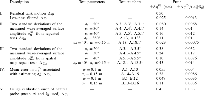
We estimate the error in the wave-averaged free surface associated with residual tank motion (error measure I) to be negligibly small ( $\pm 0.025~\text{mm}$
). The repeatability of experiments is found be extremely high (error measure II), with exact repeats of the same experiment giving an error in the maximum amplitude of the wave-averaged free surface between repeats of 0.023–0.14 mm. We define our measure of error to be two times the standard deviation in all cases. A more substantial error in the wave-averaged free surface of 0.1–0.38 mm (
$\pm 0.025~\text{mm}$
). The repeatability of experiments is found be extremely high (error measure II), with exact repeats of the same experiment giving an error in the maximum amplitude of the wave-averaged free surface between repeats of 0.023–0.14 mm. We define our measure of error to be two times the standard deviation in all cases. A more substantial error in the wave-averaged free surface of 0.1–0.38 mm ( $a_{0}=0.1~\text{m}$
) and 0.43 mm (
$a_{0}=0.1~\text{m}$
) and 0.43 mm ( $a_{0}=0.15~\text{m}$
) (two standard deviations) is identified when the same experiments are repeated, but the main direction of travel of the group is varied, reflecting slight azimuthal asymmetry in the wavemaker configuration or the gauge layout. From repeated resampling from our 14 probes we obtain an error in the wave-averaged free-surface amplitude, resulting from an error in
$a_{0}=0.15~\text{m}$
) (two standard deviations) is identified when the same experiments are repeated, but the main direction of travel of the group is varied, reflecting slight azimuthal asymmetry in the wavemaker configuration or the gauge layout. From repeated resampling from our 14 probes we obtain an error in the wave-averaged free-surface amplitude, resulting from an error in $\unicode[STIX]{x1D70E}_{\unicode[STIX]{x1D703}}^{\star }$
of 0.047–0.28 mm (
$\unicode[STIX]{x1D70E}_{\unicode[STIX]{x1D703}}^{\star }$
of 0.047–0.28 mm ( $a_{0}=0.1~\text{m}$
) and 0.3–0.7 mm (
$a_{0}=0.1~\text{m}$
) and 0.3–0.7 mm ( $a_{0}=0.15~\text{m}$
). Underlying all of these sources of error is most likely the error associated with wave gauge calibration of 0.4 mm (error measure V). As our measures of error are not independent, we take calibration error to be the dominant source of error and use this in the error bars presented in the next section. Specifically, the error bars correspond to two standard deviations either side of the mean.
$a_{0}=0.15~\text{m}$
). Underlying all of these sources of error is most likely the error associated with wave gauge calibration of 0.4 mm (error measure V). As our measures of error are not independent, we take calibration error to be the dominant source of error and use this in the error bars presented in the next section. Specifically, the error bars correspond to two standard deviations either side of the mean.
4 Results
In this section, we compare our experimental results with predictions for the wave-averaged free surface based on the parameters estimated from the linear signal in the two categories we consider: spreading tests (category A, §§ 4.1 and 4.2) and crossing tests (category B, § 4.3). Throughout this section, we compare measured and theoretically predicted surface elevations, denoted by the subscripts $M$
and
$M$
and $T$
respectively. The measured wave-averaged surface elevation
$T$
respectively. The measured wave-averaged surface elevation $\unicode[STIX]{x1D702}_{M-}^{(2)}$
is extracted from the measured time series using the process outlined in § 3.3, and its theoretical counterpart
$\unicode[STIX]{x1D702}_{M-}^{(2)}$
is extracted from the measured time series using the process outlined in § 3.3, and its theoretical counterpart $\unicode[STIX]{x1D702}_{T-}^{(2)}$
is calculated using (2.21), using as inputs the linear part of the time series measured at the central probe,
$\unicode[STIX]{x1D702}_{T-}^{(2)}$
is calculated using (2.21), using as inputs the linear part of the time series measured at the central probe, $\unicode[STIX]{x1D702}_{M}^{(1)}$
, and the estimated values of
$\unicode[STIX]{x1D702}_{M}^{(1)}$
, and the estimated values of $\unicode[STIX]{x1D70E}_{\unicode[STIX]{x1D703}}^{\star }$
reported in tables 2 and 3 for the two respective categories. Appendix D gives the original time series of the free-surface elevation measured at the central probe for completeness.
$\unicode[STIX]{x1D70E}_{\unicode[STIX]{x1D703}}^{\star }$
reported in tables 2 and 3 for the two respective categories. Appendix D gives the original time series of the free-surface elevation measured at the central probe for completeness.
4.1 Spreading tests (category A)
Beginning our discussion with the properties of the linear signal, table 2 compares input and estimated spectral parameters for the spreading tests. The estimated spreading $\unicode[STIX]{x1D70E}_{\unicode[STIX]{x1D703}}^{\star }$
is consistent with the input values of spreading
$\unicode[STIX]{x1D70E}_{\unicode[STIX]{x1D703}}^{\star }$
is consistent with the input values of spreading $\unicode[STIX]{x1D70E}_{\unicode[STIX]{x1D703}}$
. A slight offset is observed, with the estimates consistently smaller than the inputs. The increased-amplitude tests A.14–19 show a slightly larger reduction in spreading for tests at
$\unicode[STIX]{x1D70E}_{\unicode[STIX]{x1D703}}$
. A slight offset is observed, with the estimates consistently smaller than the inputs. The increased-amplitude tests A.14–19 show a slightly larger reduction in spreading for tests at $\unicode[STIX]{x1D70E}_{\unicode[STIX]{x1D703}}^{\star }=10^{\circ }$
and
$\unicode[STIX]{x1D70E}_{\unicode[STIX]{x1D703}}^{\star }=10^{\circ }$
and $\unicode[STIX]{x1D70E}_{\unicode[STIX]{x1D703}}^{\star }=20^{\circ }$
, which is consistent with the numerical simulations of Gibbs & Taylor (Reference Gibbs and Taylor2005). These authors observe a reduction in spreading proportional to the steepness
$\unicode[STIX]{x1D70E}_{\unicode[STIX]{x1D703}}^{\star }=20^{\circ }$
, which is consistent with the numerical simulations of Gibbs & Taylor (Reference Gibbs and Taylor2005). These authors observe a reduction in spreading proportional to the steepness $\unicode[STIX]{x1D6FC}^{2}$
for a degree of spreading
$\unicode[STIX]{x1D6FC}^{2}$
for a degree of spreading $\unicode[STIX]{x1D70E}_{\unicode[STIX]{x1D703}}=15^{\circ }$
. Deviations in the amplitude from the input can be attributed to either nonlinear evolution or wavemaker performance. Turning to the estimated wavenumber, we observe a slight reduction in carrier wavenumber for tests with low degrees of directional spreading (
$\unicode[STIX]{x1D70E}_{\unicode[STIX]{x1D703}}=15^{\circ }$
. Deviations in the amplitude from the input can be attributed to either nonlinear evolution or wavemaker performance. Turning to the estimated wavenumber, we observe a slight reduction in carrier wavenumber for tests with low degrees of directional spreading ( $0{-}20^{\circ }$
), as evidence of classical down-shift of the peak wavenumber, which is more pronounced for larger steepness (Lake et al.
Reference Lake, Yuen, Rungaldier and Ferguson1977; Tian, Perlin & Choi Reference Tian, Perlin and Choi2011). Consistently, the down-shift becomes less pronounced for increasing degrees of directional spreading, as the effects of spreading serve to decrease the overall degree of nonlinearity (see also Johannessen & Swan Reference Johannessen and Swan2001). There are no significant trends in the estimated bandwidth
$0{-}20^{\circ }$
), as evidence of classical down-shift of the peak wavenumber, which is more pronounced for larger steepness (Lake et al.
Reference Lake, Yuen, Rungaldier and Ferguson1977; Tian, Perlin & Choi Reference Tian, Perlin and Choi2011). Consistently, the down-shift becomes less pronounced for increasing degrees of directional spreading, as the effects of spreading serve to decrease the overall degree of nonlinearity (see also Johannessen & Swan Reference Johannessen and Swan2001). There are no significant trends in the estimated bandwidth $\unicode[STIX]{x0394}k^{\star }$
.
$\unicode[STIX]{x0394}k^{\star }$
.
Figure 8 compares the measured ( $\unicode[STIX]{x1D702}_{M-}^{(2)}$
) and theoretically predicted (
$\unicode[STIX]{x1D702}_{M-}^{(2)}$
) and theoretically predicted ( $\unicode[STIX]{x1D702}_{T-}^{(2)}$
) wave-averaged surface elevations at the central probe for tests A.1–12. Both the measured and the predicted results show a set-down for low degrees of directional spreading (a–d). As the degree of spreading is increased, the amplitude of the set-down decreases, and reaches zero at around
$\unicode[STIX]{x1D702}_{T-}^{(2)}$
) wave-averaged surface elevations at the central probe for tests A.1–12. Both the measured and the predicted results show a set-down for low degrees of directional spreading (a–d). As the degree of spreading is increased, the amplitude of the set-down decreases, and reaches zero at around $\unicode[STIX]{x1D70E}_{\unicode[STIX]{x1D703}}^{\star }\approx 40^{\circ }$
(e), after which a set-up begins to form (f–l). The measured and predicted wave-averaged surface elevations show very good agreement, with best agreement for low and high degrees of spreading. At the extremes
$\unicode[STIX]{x1D70E}_{\unicode[STIX]{x1D703}}^{\star }\approx 40^{\circ }$
(e), after which a set-up begins to form (f–l). The measured and predicted wave-averaged surface elevations show very good agreement, with best agreement for low and high degrees of spreading. At the extremes $\unicode[STIX]{x1D70E}_{\unicode[STIX]{x1D703}}\rightarrow 0$
and
$\unicode[STIX]{x1D70E}_{\unicode[STIX]{x1D703}}\rightarrow 0$
and $\unicode[STIX]{x1D70E}_{\unicode[STIX]{x1D703}}\rightarrow \infty$
, it is straightforward to accurately estimate the spreading. The slight decrease in agreement for intermediate values of
$\unicode[STIX]{x1D70E}_{\unicode[STIX]{x1D703}}\rightarrow \infty$
, it is straightforward to accurately estimate the spreading. The slight decrease in agreement for intermediate values of $\unicode[STIX]{x1D70E}_{\unicode[STIX]{x1D703}}^{\star }$
is probably indicative of uncertainty associated with estimation of
$\unicode[STIX]{x1D70E}_{\unicode[STIX]{x1D703}}^{\star }$
is probably indicative of uncertainty associated with estimation of $\unicode[STIX]{x1D70E}_{\unicode[STIX]{x1D703}}^{\star }$
in this regime. In all cases, the differences between the measured and the predicted values lie well within the approximate error bounds estimated in § 3.6. At higher values of steepness, figure 9 shows improved agreement between the measurements and the predictions in the range
$\unicode[STIX]{x1D70E}_{\unicode[STIX]{x1D703}}^{\star }$
in this regime. In all cases, the differences between the measured and the predicted values lie well within the approximate error bounds estimated in § 3.6. At higher values of steepness, figure 9 shows improved agreement between the measurements and the predictions in the range $\unicode[STIX]{x1D70E}_{\unicode[STIX]{x1D703}}=0{-}50^{\circ }$
(tests A.14–19), especially for intermediate degrees of spreading.
$\unicode[STIX]{x1D70E}_{\unicode[STIX]{x1D703}}=0{-}50^{\circ }$
(tests A.14–19), especially for intermediate degrees of spreading.

Figure 8. The wave-averaged surface elevation $\unicode[STIX]{x1D702}_{-}^{(2)}$
at the central probe (
$\unicode[STIX]{x1D702}_{-}^{(2)}$
at the central probe ( $x=0$
,
$x=0$
, $y=0$
) for the spreading tests (category A), showing measurements
$y=0$
) for the spreading tests (category A), showing measurements $\unicode[STIX]{x1D702}_{M-}^{(2)}$
(black lines) and theoretical predictions
$\unicode[STIX]{x1D702}_{M-}^{(2)}$
(black lines) and theoretical predictions $\unicode[STIX]{x1D702}_{T-}^{(2)}$
(red dashed lines) for an input amplitude of
$\unicode[STIX]{x1D702}_{T-}^{(2)}$
(red dashed lines) for an input amplitude of $a_{0}=0.1~\text{m}$
. The different panels correspond to increasing degree of input spreading
$a_{0}=0.1~\text{m}$
. The different panels correspond to increasing degree of input spreading $\unicode[STIX]{x1D70E}_{\unicode[STIX]{x1D703}}=0$
–
$\unicode[STIX]{x1D70E}_{\unicode[STIX]{x1D703}}=0$
– $180^{\circ }$
(see table 2) and the labels denote the estimated degree of spreading
$180^{\circ }$
(see table 2) and the labels denote the estimated degree of spreading $\unicode[STIX]{x1D70E}_{\unicode[STIX]{x1D703}}^{\star }$
used for the theoretical predictions of
$\unicode[STIX]{x1D70E}_{\unicode[STIX]{x1D703}}^{\star }$
used for the theoretical predictions of $\unicode[STIX]{x1D702}_{T-}^{(2)}$
.
$\unicode[STIX]{x1D702}_{T-}^{(2)}$
.

Figure 9. The wave-averaged surface elevation $\unicode[STIX]{x1D702}_{-}^{(2)}$
at the central probe (
$\unicode[STIX]{x1D702}_{-}^{(2)}$
at the central probe ( $x=0$
,
$x=0$
, $y=0$
) for the spreading tests (category A), showing measurements
$y=0$
) for the spreading tests (category A), showing measurements $\unicode[STIX]{x1D702}_{M-}^{(2)}$
(black lines) and theoretical predictions
$\unicode[STIX]{x1D702}_{M-}^{(2)}$
(black lines) and theoretical predictions $\unicode[STIX]{x1D702}_{T-}^{(2)}$
(red dashed lines) for a linear input amplitude of
$\unicode[STIX]{x1D702}_{T-}^{(2)}$
(red dashed lines) for a linear input amplitude of $a_{0}=0.15~\text{m}$
. The different panels correspond to increasing degree of input spreading
$a_{0}=0.15~\text{m}$
. The different panels correspond to increasing degree of input spreading $\unicode[STIX]{x1D70E}_{\unicode[STIX]{x1D703}}=0$
–
$\unicode[STIX]{x1D70E}_{\unicode[STIX]{x1D703}}=0$
– $50^{\circ }$
(see table 2) and the labels denote the estimated degree of spreading
$50^{\circ }$
(see table 2) and the labels denote the estimated degree of spreading $\unicode[STIX]{x1D70E}_{\unicode[STIX]{x1D703}}^{\star }$
.
$\unicode[STIX]{x1D70E}_{\unicode[STIX]{x1D703}}^{\star }$
.
Figure 10 summarizes the results of the spreading tests. Panel (a) compares the amplitude of the measured wave-averaged surface elevation $a_{M-}^{(2)}$
with the theoretical prediction
$a_{M-}^{(2)}$
with the theoretical prediction $a_{T-}^{(2)}$
calculated from (2.21). The values of
$a_{T-}^{(2)}$
calculated from (2.21). The values of $a_{T-}^{(2)}$
in this panel rely on the measured linear spectra, as in figures 8 and 9. Accordingly, we note that the increased-steepness experiments compare with theory slightly better. In order to compute the theoretical line in (a), we must specify a single amplitude distribution
$a_{T-}^{(2)}$
in this panel rely on the measured linear spectra, as in figures 8 and 9. Accordingly, we note that the increased-steepness experiments compare with theory slightly better. In order to compute the theoretical line in (a), we must specify a single amplitude distribution $\hat{\unicode[STIX]{x1D702}}(k)$
, despite slight variations in
$\hat{\unicode[STIX]{x1D702}}(k)$
, despite slight variations in $k_{0}^{\star }$
and
$k_{0}^{\star }$
and $\unicode[STIX]{x0394}k^{\star }$
between experiments (cf. table 2). The red lines in figure 10(b) show the amplitude of the wave-averaged surface elevation for a Gaussian amplitude distribution (3.1) with
$\unicode[STIX]{x0394}k^{\star }$
between experiments (cf. table 2). The red lines in figure 10(b) show the amplitude of the wave-averaged surface elevation for a Gaussian amplitude distribution (3.1) with $k_{0}=1.90~\text{m}^{-1}$
and
$k_{0}=1.90~\text{m}^{-1}$
and $\unicode[STIX]{x0394}k=0.60~\text{m}^{-1}$
. The dotted line, denoted by
$\unicode[STIX]{x0394}k=0.60~\text{m}^{-1}$
. The dotted line, denoted by $\unicode[STIX]{x1D716}_{x}\rightarrow 0$
, corresponds to the multiple-scale approximation (2.8), whereas the dashed line corresponds to the multiple-component solution (2.21). Both lines rely on the same Gaussian directional distribution. It is evident from comparing these two lines that both approaches agree for small degrees of directional spreading, noting a slight underestimation of the magnitude of the set-down by the multiple-scale approximation (
$\unicode[STIX]{x1D716}_{x}\rightarrow 0$
, corresponds to the multiple-scale approximation (2.8), whereas the dashed line corresponds to the multiple-component solution (2.21). Both lines rely on the same Gaussian directional distribution. It is evident from comparing these two lines that both approaches agree for small degrees of directional spreading, noting a slight underestimation of the magnitude of the set-down by the multiple-scale approximation ( $\unicode[STIX]{x1D716}_{x}=0.3$
). For larger degrees of directional spreading, the multiple-scale solution fails, as expected.
$\unicode[STIX]{x1D716}_{x}=0.3$
). For larger degrees of directional spreading, the multiple-scale solution fails, as expected.

Figure 10. The amplitude of the wave-averaged surface elevation at the central probe ( $x=0$
,
$x=0$
, $y=0$
) for the spreading tests (category A); (a) shows the measured wave-averaged surface amplitude
$y=0$
) for the spreading tests (category A); (a) shows the measured wave-averaged surface amplitude $a_{M-}^{(2)}$
as a function of the theoretical prediction
$a_{M-}^{(2)}$
as a function of the theoretical prediction $a_{T-}^{(2)}$
, with error bars shown in grey (see § 3.6 and appendix C for details), and (b) shows the measured amplitude
$a_{T-}^{(2)}$
, with error bars shown in grey (see § 3.6 and appendix C for details), and (b) shows the measured amplitude $a_{M-}^{(2)}$
as a function of the estimated degree of spreading
$a_{M-}^{(2)}$
as a function of the estimated degree of spreading $\unicode[STIX]{x1D70E}_{\unicode[STIX]{x1D703}}^{\star }$
. The red dashed lines correspond to a perfectly focused Gaussian wave group.
$\unicode[STIX]{x1D70E}_{\unicode[STIX]{x1D703}}^{\star }$
. The red dashed lines correspond to a perfectly focused Gaussian wave group.
4.2 Spreading tests (category A): spatial measurements
Beginning our discussion again with the properties of the linear signal, the estimated spectral parameters for the repeat tests carried out in producing spatial measurements are evidently consistent with those for the analogous tests discussed before (tests A.3–5,18). As we change the direction of travel of the wave group $\unicode[STIX]{x1D703}_{0}$
from
$\unicode[STIX]{x1D703}_{0}$
from $0$
to
$0$
to $90^{\circ }$
, leaving the gauge array fixed, we can observe that our estimate of
$90^{\circ }$
, leaving the gauge array fixed, we can observe that our estimate of $\unicode[STIX]{x1D70E}_{\unicode[STIX]{x1D703}}^{\star }$
varies by
$\unicode[STIX]{x1D70E}_{\unicode[STIX]{x1D703}}^{\star }$
varies by $1.2^{\circ }$
at most. This variation is less for the increased-amplitude tests, with
$1.2^{\circ }$
at most. This variation is less for the increased-amplitude tests, with $\unicode[STIX]{x1D70E}_{\unicode[STIX]{x1D703}}^{\star }$
only varying by
$\unicode[STIX]{x1D70E}_{\unicode[STIX]{x1D703}}^{\star }$
only varying by $0.4^{\circ }$
. In order to assess how well the directional spectrum is reproduced by the wavemakers, figure 11 compares the measured linear free surface
$0.4^{\circ }$
. In order to assess how well the directional spectrum is reproduced by the wavemakers, figure 11 compares the measured linear free surface $\unicode[STIX]{x1D702}_{M}^{(1)}$
shown in the top half with the predicted linear surface
$\unicode[STIX]{x1D702}_{M}^{(1)}$
shown in the top half with the predicted linear surface $\unicode[STIX]{x1D702}_{T}^{(1)}$
at the same gauges mirrored in the bottom half, all at the time of focus. The predicted linear free surface compares very well with measurements, illustrating that our approach is capable of accurately measuring the spatial free-surface elevation and that our estimates of
$\unicode[STIX]{x1D702}_{T}^{(1)}$
at the same gauges mirrored in the bottom half, all at the time of focus. The predicted linear free surface compares very well with measurements, illustrating that our approach is capable of accurately measuring the spatial free-surface elevation and that our estimates of $\unicode[STIX]{x1D70E}_{\unicode[STIX]{x1D703}}^{\star }$
are correct.
$\unicode[STIX]{x1D70E}_{\unicode[STIX]{x1D703}}^{\star }$
are correct.
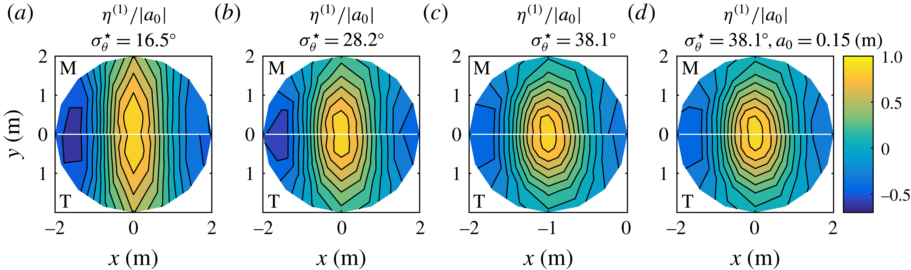
Figure 11. Contours comparing the measured linear free surface $\unicode[STIX]{x1D702}_{M}^{(1)}$
(top half) and the predicted linear surface
$\unicode[STIX]{x1D702}_{M}^{(1)}$
(top half) and the predicted linear surface $\unicode[STIX]{x1D702}_{T}^{(1)}$
(bottom half) at time of focus; (a)–(c) correspond to increasing degree of input spreading
$\unicode[STIX]{x1D702}_{T}^{(1)}$
(bottom half) at time of focus; (a)–(c) correspond to increasing degree of input spreading $\unicode[STIX]{x1D70E}_{\unicode[STIX]{x1D703}}=20,30,40^{\circ }$
(for
$\unicode[STIX]{x1D70E}_{\unicode[STIX]{x1D703}}=20,30,40^{\circ }$
(for $a_{0}=0.1~\text{m}$
) and the labels give the estimated degree of spreading
$a_{0}=0.1~\text{m}$
) and the labels give the estimated degree of spreading $\unicode[STIX]{x1D70E}_{\unicode[STIX]{x1D703}}^{\star }$
used for theoretical predictions of
$\unicode[STIX]{x1D70E}_{\unicode[STIX]{x1D703}}^{\star }$
used for theoretical predictions of $\unicode[STIX]{x1D702}_{T}^{(1)}$
; (d) corresponds to an increased amplitude
$\unicode[STIX]{x1D702}_{T}^{(1)}$
; (d) corresponds to an increased amplitude $a_{0}=0.15~\text{m}$
at
$a_{0}=0.15~\text{m}$
at $\unicode[STIX]{x1D70E}_{\unicode[STIX]{x1D703}}=40^{\circ }$
. Only positive values of
$\unicode[STIX]{x1D70E}_{\unicode[STIX]{x1D703}}=40^{\circ }$
. Only positive values of $y$
are shown and the white horizontal lines demarcate the measured linear free surface shown in the top half (labelled
$y$
are shown and the white horizontal lines demarcate the measured linear free surface shown in the top half (labelled $M$
) and the theoretically predicted linear free surface shown in the bottom half (labelled
$M$
) and the theoretically predicted linear free surface shown in the bottom half (labelled $T$
).
$T$
).
The two-dimensional structure of the wave-averaged surface elevation is examined in figure 12. Panels (a–c) show the measured wave-averaged surface elevation $\unicode[STIX]{x1D702}_{M-}^{(2)}$
as input spreading is increased from
$\unicode[STIX]{x1D702}_{M-}^{(2)}$
as input spreading is increased from $20{-}40^{\circ }$
, and (d) shows the increased-amplitude test with
$20{-}40^{\circ }$
, and (d) shows the increased-amplitude test with $\unicode[STIX]{x1D70E}_{\unicode[STIX]{x1D703}}=40^{\circ }$
. For (a–d), the measured surface
$\unicode[STIX]{x1D70E}_{\unicode[STIX]{x1D703}}=40^{\circ }$
. For (a–d), the measured surface $\unicode[STIX]{x1D702}_{M-}^{(2)}$
in the south-west quadrant (
$\unicode[STIX]{x1D702}_{M-}^{(2)}$
in the south-west quadrant ( $x<0$
,
$x<0$
, $y<0$
) is mirrored from the north-west quadrant (
$y<0$
) is mirrored from the north-west quadrant ( $x<0$
,
$x<0$
, $y>0$
), assuming symmetry, in order to complete the surface measured by our asymmetric gauge array. Panels (e–h) show the predicted wave-averaged surface elevation
$y>0$
), assuming symmetry, in order to complete the surface measured by our asymmetric gauge array. Panels (e–h) show the predicted wave-averaged surface elevation $\unicode[STIX]{x1D702}_{T-}^{(2)}$
(calculated using
$\unicode[STIX]{x1D702}_{T-}^{(2)}$
(calculated using $\unicode[STIX]{x1D70E}_{\unicode[STIX]{x1D703}}^{\star }$
). The set-down can clearly be observed as a deep hole that reduces with increasing spreading by the formation of the set-up, eventually splitting into two holes either side of the wave crest, which is now enhanced by a set-up ridge. The agreement is better for the increased-amplitude experiment in (d,h). For each test, the holes are slightly deeper than predicted and the set-up is slightly less pronounced, all within the bounds of experimental error. The formation of the set-up ridge is clearly captured. It is worth noting that the array of probes used to generate these contours is sparse around the point of focus (
$\unicode[STIX]{x1D70E}_{\unicode[STIX]{x1D703}}^{\star }$
). The set-down can clearly be observed as a deep hole that reduces with increasing spreading by the formation of the set-up, eventually splitting into two holes either side of the wave crest, which is now enhanced by a set-up ridge. The agreement is better for the increased-amplitude experiment in (d,h). For each test, the holes are slightly deeper than predicted and the set-up is slightly less pronounced, all within the bounds of experimental error. The formation of the set-up ridge is clearly captured. It is worth noting that the array of probes used to generate these contours is sparse around the point of focus ( $x=0$
,
$x=0$
, $y=0$
) (see figure 7). Therefore, any error in this area is exaggerated when linear interpolation is used to produce the contour surfaces.
$y=0$
) (see figure 7). Therefore, any error in this area is exaggerated when linear interpolation is used to produce the contour surfaces.

Figure 12. Contour plots showing the measured wave-averaged surface elevation $\unicode[STIX]{x1D702}_{M-}^{(2)}$
(a–d) and the predicted wave-averaged surface elevation
$\unicode[STIX]{x1D702}_{M-}^{(2)}$
(a–d) and the predicted wave-averaged surface elevation $\unicode[STIX]{x1D702}_{T-}^{(2)}$
(e–h) at time of focus; (a–c,e–g) correspond to increasing degree of input spreading
$\unicode[STIX]{x1D702}_{T-}^{(2)}$
(e–h) at time of focus; (a–c,e–g) correspond to increasing degree of input spreading $\unicode[STIX]{x1D70E}_{\unicode[STIX]{x1D703}}=20,30,40^{\circ }$
(for
$\unicode[STIX]{x1D70E}_{\unicode[STIX]{x1D703}}=20,30,40^{\circ }$
(for $a_{0}=0.1~\text{m}$
) and (d,h) correspond to an increased amplitude
$a_{0}=0.1~\text{m}$
) and (d,h) correspond to an increased amplitude $a_{0}=0.15~\text{m}$
at
$a_{0}=0.15~\text{m}$
at $\unicode[STIX]{x1D70E}_{\unicode[STIX]{x1D703}}=40^{\circ }$
. The labels in (e–h) give the estimated degree of spreading
$\unicode[STIX]{x1D70E}_{\unicode[STIX]{x1D703}}=40^{\circ }$
. The labels in (e–h) give the estimated degree of spreading $\unicode[STIX]{x1D70E}_{\unicode[STIX]{x1D703}}^{\star }$
used for theoretical predictions of
$\unicode[STIX]{x1D70E}_{\unicode[STIX]{x1D703}}^{\star }$
used for theoretical predictions of $\unicode[STIX]{x1D702}_{T}^{(1)}$
(see the supplementary material online available at https://doi.org/10.1017/jfm.2017.774 for animations of
$\unicode[STIX]{x1D702}_{T}^{(1)}$
(see the supplementary material online available at https://doi.org/10.1017/jfm.2017.774 for animations of $\unicode[STIX]{x1D702}_{M-}^{(2)}(x,y,t)$
).
$\unicode[STIX]{x1D702}_{M-}^{(2)}(x,y,t)$
).
4.3 Crossing group tests (category B)
Beginning our discussion with the properties of the linear signal as before, estimated spectral parameters for the crossing tests are reported in table 3. We note that the amplitude refers to the combined linear amplitude of the two groups. As the steepness of the individual groups before they meet is thus halved, this could perhaps explain the reduction in the (small) deviation between input and estimated spreading, and input and estimated carrier wavenumber. Both are associated with nonlinearity, respectively through the phenomena of spectral down-shift and narrowing of the group observed in numerical simulations by Gibbs & Taylor (Reference Gibbs and Taylor2005).
Figure 13 compares the measured ( $\unicode[STIX]{x1D702}_{M-}^{(2)}$
) and theoretically predicted (
$\unicode[STIX]{x1D702}_{M-}^{(2)}$
) and theoretically predicted ( $\unicode[STIX]{x1D702}_{T-}^{(2)}$
) wave-averaged surface elevations at the central probe for tests B.1–16. For all degrees of spreading and a crossing angle of
$\unicode[STIX]{x1D702}_{T-}^{(2)}$
) wave-averaged surface elevations at the central probe for tests B.1–16. For all degrees of spreading and a crossing angle of $\unicode[STIX]{x0394}\unicode[STIX]{x1D703}=45^{\circ }$
, a small set-down is observed. When the crossing angle is increased to
$\unicode[STIX]{x0394}\unicode[STIX]{x1D703}=45^{\circ }$
, a small set-down is observed. When the crossing angle is increased to $90^{\circ }$
, a significant set-up can be observed for all degrees of spreading, growing to a maximum value at a crossing angle of
$90^{\circ }$
, a significant set-up can be observed for all degrees of spreading, growing to a maximum value at a crossing angle of $\unicode[STIX]{x0394}\unicode[STIX]{x1D703}=180^{\circ }$
. The measured and predicted wave-averaged surface elevations again show remarkable agreement, with even better agreement for higher crossing angles.
$\unicode[STIX]{x0394}\unicode[STIX]{x1D703}=180^{\circ }$
. The measured and predicted wave-averaged surface elevations again show remarkable agreement, with even better agreement for higher crossing angles.

Figure 13. The wave-averaged surface elevation $\unicode[STIX]{x1D702}_{-}^{(2)}$
at the central probe (
$\unicode[STIX]{x1D702}_{-}^{(2)}$
at the central probe ( $x=0$
,
$x=0$
, $y=0$
) for the crossing tests (category B), showing measurements
$y=0$
) for the crossing tests (category B), showing measurements $\unicode[STIX]{x1D702}_{M-}^{(2)}$
(black lines) and theoretical predictions
$\unicode[STIX]{x1D702}_{M-}^{(2)}$
(black lines) and theoretical predictions $\unicode[STIX]{x1D702}_{T-}^{(2)}$
(red dashed lines) for an input amplitude of
$\unicode[STIX]{x1D702}_{T-}^{(2)}$
(red dashed lines) for an input amplitude of $a_{0}=0.1~\text{m}$
, for different values of the crossing angle
$a_{0}=0.1~\text{m}$
, for different values of the crossing angle $\unicode[STIX]{x0394}\unicode[STIX]{x1D703}=0$
–
$\unicode[STIX]{x0394}\unicode[STIX]{x1D703}=0$
– $180^{\circ }$
and the degree of input spreading
$180^{\circ }$
and the degree of input spreading $\unicode[STIX]{x1D70E}_{\unicode[STIX]{x1D703}}=10,20,30^{\circ }$
(a–d,e–h,i–l), with estimated values
$\unicode[STIX]{x1D70E}_{\unicode[STIX]{x1D703}}=10,20,30^{\circ }$
(a–d,e–h,i–l), with estimated values $\unicode[STIX]{x1D70E}_{\unicode[STIX]{x1D703}}^{\star }$
reported in the labels (see table 3); (m–p) correspond to increased-amplitude experiments at
$\unicode[STIX]{x1D70E}_{\unicode[STIX]{x1D703}}^{\star }$
reported in the labels (see table 3); (m–p) correspond to increased-amplitude experiments at $a_{0}=0.15~\text{m}$
.
$a_{0}=0.15~\text{m}$
.
In the absence of full surface measurements, figure 14 compares measured and theoretical wave-averaged surface elevations along the $x$
-axis, where nine probes are located. There is good agreement between the measurements,
$x$
-axis, where nine probes are located. There is good agreement between the measurements, $\unicode[STIX]{x1D702}_{M-}^{(2)}$
(black dots), and the multiple-component solution (2.21) (red dashed lines) in all cases. The multiple-scale solution for two crossing groups (2.15) (continuous black lines) is computed under the assumption of perfectly focused Gaussian wave groups (
$\unicode[STIX]{x1D702}_{M-}^{(2)}$
(black dots), and the multiple-component solution (2.21) (red dashed lines) in all cases. The multiple-scale solution for two crossing groups (2.15) (continuous black lines) is computed under the assumption of perfectly focused Gaussian wave groups ( $\unicode[STIX]{x1D707}_{1}=\unicode[STIX]{x1D707}_{2}=0$
) and is somewhat larger than the multiple-component solution. Nevertheless, the measured wave-averaged surface elevation is well captured by the multiple-scale solution, except for low crossing angles (
$\unicode[STIX]{x1D707}_{1}=\unicode[STIX]{x1D707}_{2}=0$
) and is somewhat larger than the multiple-component solution. Nevertheless, the measured wave-averaged surface elevation is well captured by the multiple-scale solution, except for low crossing angles ( $\unicode[STIX]{x0394}\unicode[STIX]{x1D703}=45^{\circ }$
), where the azimuthal distribution is not well separated. Crucially, it is evident from figure 14 that for higher crossing angles, all of the wave-averaged surface elevations exhibit a rapidly varying local structure, which differs drastically from the slow hole or hump formed by an individual wave group. As captured by (2.19), the crossing wave pattern consists of a modulated wave group with its peak coinciding with the main linear crest for two wave groups that are in phase (
$\unicode[STIX]{x0394}\unicode[STIX]{x1D703}=45^{\circ }$
), where the azimuthal distribution is not well separated. Crucially, it is evident from figure 14 that for higher crossing angles, all of the wave-averaged surface elevations exhibit a rapidly varying local structure, which differs drastically from the slow hole or hump formed by an individual wave group. As captured by (2.19), the crossing wave pattern consists of a modulated wave group with its peak coinciding with the main linear crest for two wave groups that are in phase ( $\unicode[STIX]{x1D707}_{1}=\unicode[STIX]{x1D707}_{2}=0$
). The set-up crest, in turn, is part of a wider ridge along the bisection of the directions of travel of the two groups.
$\unicode[STIX]{x1D707}_{1}=\unicode[STIX]{x1D707}_{2}=0$
). The set-up crest, in turn, is part of a wider ridge along the bisection of the directions of travel of the two groups.

Figure 14. The wave-averaged surface elevation $\unicode[STIX]{x1D702}_{-}^{(2)}$
in the direction of propagation (
$\unicode[STIX]{x1D702}_{-}^{(2)}$
in the direction of propagation ( $y=0$
) at the time of linear focus for the crossing tests (category B), showing measurements
$y=0$
) at the time of linear focus for the crossing tests (category B), showing measurements $\unicode[STIX]{x1D702}_{M-}^{(2)}$
(black dots), theoretical predictions
$\unicode[STIX]{x1D702}_{M-}^{(2)}$
(black dots), theoretical predictions $\unicode[STIX]{x1D702}_{T-}^{(2)}$
made using the multiple-component solution (2.21) (red dashed lines) and using the multiple-scale solution (2.15) (continuous black lines) for an input amplitude of
$\unicode[STIX]{x1D702}_{T-}^{(2)}$
made using the multiple-component solution (2.21) (red dashed lines) and using the multiple-scale solution (2.15) (continuous black lines) for an input amplitude of $a_{0}=0.1~\text{m}$
, for different values of the crossing angle
$a_{0}=0.1~\text{m}$
, for different values of the crossing angle $\unicode[STIX]{x0394}\unicode[STIX]{x1D703}=0$
–
$\unicode[STIX]{x0394}\unicode[STIX]{x1D703}=0$
– $180^{\circ }$
and the degree of input spreading
$180^{\circ }$
and the degree of input spreading $\unicode[STIX]{x1D70E}_{\unicode[STIX]{x1D703}}=10,20,30^{\circ }$
(a–d,e–h,i–l), with estimated values
$\unicode[STIX]{x1D70E}_{\unicode[STIX]{x1D703}}=10,20,30^{\circ }$
(a–d,e–h,i–l), with estimated values $\unicode[STIX]{x1D70E}_{\unicode[STIX]{x1D703}}^{\star }$
reported in the labels; (m–p) correspond to increased-amplitude experiments at
$\unicode[STIX]{x1D70E}_{\unicode[STIX]{x1D703}}^{\star }$
reported in the labels; (m–p) correspond to increased-amplitude experiments at $a_{0}=0.15~\text{m}$
.
$a_{0}=0.15~\text{m}$
.
4.3.1 The role of phase
Examining the role of phase more carefully, figure 15 compares the wave-averaged free surfaces for two opposing unidirectional wave groups ( $\unicode[STIX]{x0394}\unicode[STIX]{x1D703}=180^{\circ }$
) that are in phase (
$\unicode[STIX]{x0394}\unicode[STIX]{x1D703}=180^{\circ }$
) that are in phase ( $\unicode[STIX]{x1D707}_{1}=\unicode[STIX]{x1D707}_{2}$
) and out of phase (
$\unicode[STIX]{x1D707}_{1}=\unicode[STIX]{x1D707}_{2}$
) and out of phase ( $\unicode[STIX]{x1D707}_{1}-\unicode[STIX]{x1D707}_{2}=180^{\circ }$
). When the phase of one group is shifted by
$\unicode[STIX]{x1D707}_{1}-\unicode[STIX]{x1D707}_{2}=180^{\circ }$
). When the phase of one group is shifted by $180^{\circ }$
, the wave-averaged surface elevation is reversed, becoming negative, as predicted by (2.15). It is also evident from this figure that the ‘hole’ is deeper than the ‘hump’, as the set-down is not a function of phase and always remains negative, while the crossing wave contribution changes sign. Nevertheless, it is worth emphasizing that in the in-phase case (
$180^{\circ }$
, the wave-averaged surface elevation is reversed, becoming negative, as predicted by (2.15). It is also evident from this figure that the ‘hole’ is deeper than the ‘hump’, as the set-down is not a function of phase and always remains negative, while the crossing wave contribution changes sign. Nevertheless, it is worth emphasizing that in the in-phase case ( $\unicode[STIX]{x1D707}_{1}=\unicode[STIX]{x1D707}_{2}$
), the linear signal constructively interferes and the ‘hump’ contributes to an already large and positive crest, whereas in the out-of-phase case (
$\unicode[STIX]{x1D707}_{1}=\unicode[STIX]{x1D707}_{2}$
), the linear signal constructively interferes and the ‘hump’ contributes to an already large and positive crest, whereas in the out-of-phase case ( $\unicode[STIX]{x1D707}_{1}-\unicode[STIX]{x1D707}_{2}=180^{\circ }$
), the linear signal deconstructively interferes and the ‘hole’ combined with second-order sum components (see appendix E) is the only observable feature. Finally, due to its (partial) standing-wave nature, the set-up varies slowly in time (a), while varying rapidly in space. In time and space, it is subject to the same slow modulation associated with the product of the crossing groups, which travel at twice the group velocity from the perspective of a stationary observer.
$\unicode[STIX]{x1D707}_{1}-\unicode[STIX]{x1D707}_{2}=180^{\circ }$
), the linear signal deconstructively interferes and the ‘hole’ combined with second-order sum components (see appendix E) is the only observable feature. Finally, due to its (partial) standing-wave nature, the set-up varies slowly in time (a), while varying rapidly in space. In time and space, it is subject to the same slow modulation associated with the product of the crossing groups, which travel at twice the group velocity from the perspective of a stationary observer.

Figure 15. Temporal (a) and spatial (b) evolution of the wave-averaged surface elevation $\unicode[STIX]{x1D702}_{-}^{(2)}$
at the focus point (
$\unicode[STIX]{x1D702}_{-}^{(2)}$
at the focus point ( $x=0$
,
$x=0$
, $y=0$
) for two wave groups colliding head-on (
$y=0$
) for two wave groups colliding head-on ( $\unicode[STIX]{x0394}\unicode[STIX]{x1D703}=180^{\circ }$
). The red lines correspond to two groups that are in phase (
$\unicode[STIX]{x0394}\unicode[STIX]{x1D703}=180^{\circ }$
). The red lines correspond to two groups that are in phase ( $\unicode[STIX]{x1D707}_{1}=\unicode[STIX]{x1D707}_{2}$
) and the black lines to groups that are out of phase (
$\unicode[STIX]{x1D707}_{1}=\unicode[STIX]{x1D707}_{2}$
) and the black lines to groups that are out of phase ( $\unicode[STIX]{x1D707}_{1}-\unicode[STIX]{x1D707}_{2}=180^{\circ }$
). The multiple-scale solution (2.15) is given by the continuous lines, and the measurements by the dashed lines in (a) and the dots in (b).
$\unicode[STIX]{x1D707}_{1}-\unicode[STIX]{x1D707}_{2}=180^{\circ }$
). The multiple-scale solution (2.15) is given by the continuous lines, and the measurements by the dashed lines in (a) and the dots in (b).
Finally, figure 16 summarizes the results of the crossing tests. In (a), the amplitude of the measured wave-averaged surface elevation $a_{M-}^{(2)}$
is shown as a function of the theoretically predicted amplitude
$a_{M-}^{(2)}$
is shown as a function of the theoretically predicted amplitude $a_{T-}^{(2)}$
, showing good agreement. In (b), the amplitude of the measured wave-averaged surface elevation
$a_{T-}^{(2)}$
, showing good agreement. In (b), the amplitude of the measured wave-averaged surface elevation $a_{M-}^{(2)}$
is shown as a function of the crossing angle
$a_{M-}^{(2)}$
is shown as a function of the crossing angle $\unicode[STIX]{x0394}\unicode[STIX]{x1D703}$
. As before, in order to compute the theoretical line in (a), we must specify a single amplitude distribution
$\unicode[STIX]{x0394}\unicode[STIX]{x1D703}$
. As before, in order to compute the theoretical line in (a), we must specify a single amplitude distribution $\hat{\unicode[STIX]{x1D702}}(k)$
, despite slight variations in
$\hat{\unicode[STIX]{x1D702}}(k)$
, despite slight variations in $k_{0}^{\star }$
and
$k_{0}^{\star }$
and $\unicode[STIX]{x0394}k^{\star }$
between experiments (cf. table 2). The red dashed lines show the amplitude of the wave-averaged surface elevation for two Gaussian wave groups with
$\unicode[STIX]{x0394}k^{\star }$
between experiments (cf. table 2). The red dashed lines show the amplitude of the wave-averaged surface elevation for two Gaussian wave groups with $k_{0}=1.90~\text{m}^{-1}$
and
$k_{0}=1.90~\text{m}^{-1}$
and $\unicode[STIX]{x0394}k=0.60~\text{m}^{-1}$
for degrees of spreading
$\unicode[STIX]{x0394}k=0.60~\text{m}^{-1}$
for degrees of spreading $\unicode[STIX]{x1D70E}_{\unicode[STIX]{x1D703}}=10,20,30^{\circ }$
.
$\unicode[STIX]{x1D70E}_{\unicode[STIX]{x1D703}}=10,20,30^{\circ }$
.
5 Conclusions
Herein, we have examined the formation of a set-down or set-up of the wave-averaged free surface for compact directionally spread and crossing wave groups on deep water ( $k_{0}d\gg 1$
). We compare detailed measurements conducted at the fully directional FloWave Ocean Energy Research Facility at the University of Edinburgh with existing multiple-component second-order wave theory (Sharma & Dean Reference Sharma and Dean1981; Dalzell Reference Dalzell1999; Forristall Reference Forristall2000) and derive new results using a multiple-scale approach which lend greater insight into the problem. We believe that ours is the first experimental observation of set-up for highly directionally spread and crossing groups, following field observations of a set-up underneath the famous Draupner rogue wave (Walker et al.
Reference Walker, Taylor and Eatock Taylor2004) and on Lake George, Australia (Toffoli et al.
Reference Toffoli, Monbaliu, Onorato, Osborne, Babanin and Bitner-Gregersen2007).
$k_{0}d\gg 1$
). We compare detailed measurements conducted at the fully directional FloWave Ocean Energy Research Facility at the University of Edinburgh with existing multiple-component second-order wave theory (Sharma & Dean Reference Sharma and Dean1981; Dalzell Reference Dalzell1999; Forristall Reference Forristall2000) and derive new results using a multiple-scale approach which lend greater insight into the problem. We believe that ours is the first experimental observation of set-up for highly directionally spread and crossing groups, following field observations of a set-up underneath the famous Draupner rogue wave (Walker et al.
Reference Walker, Taylor and Eatock Taylor2004) and on Lake George, Australia (Toffoli et al.
Reference Toffoli, Monbaliu, Onorato, Osborne, Babanin and Bitner-Gregersen2007).
For a single directionally spread wave group, the total wave-averaged free surface is made up from the combination of a set-down and a set-up, which vary slowly in time but have very different spatial structures. For a perfectly focused wave group and at the centre of the group at the time of focus, the sign of the wave-averaged free surface changes for degrees of directional spreading $\unicode[STIX]{x1D70E}_{\unicode[STIX]{x1D703}}=30{-}40^{\circ }$
, which corresponds to more commonly reported degrees of spreading of the energy spectrum of
$\unicode[STIX]{x1D70E}_{\unicode[STIX]{x1D703}}=30{-}40^{\circ }$
, which corresponds to more commonly reported degrees of spreading of the energy spectrum of $\unicode[STIX]{x1D70E}_{\unicode[STIX]{x1D703}}/\sqrt{2}=21{-}28^{\circ }$
. The set-down inherits the shape of the group envelope, albeit wider due to the remote recoil of the underlying return flow that causes it, which also occurs for three-dimensional internal wave groups (Bühler & McIntyre Reference Bühler and McIntyre2003). The magnitude of the set-down reduces monotonically with an increasing degree of directional spreading. As the degree of directional spreading increases, the set-up, which is zero for unidirectional seas, forms a ridge through the set-down ‘hole’ which is aligned in the main direction of propagation of the group. The set-up is in fact part of a crossing wave pattern, which may be modulated by the presence of groups.
$\unicode[STIX]{x1D70E}_{\unicode[STIX]{x1D703}}/\sqrt{2}=21{-}28^{\circ }$
. The set-down inherits the shape of the group envelope, albeit wider due to the remote recoil of the underlying return flow that causes it, which also occurs for three-dimensional internal wave groups (Bühler & McIntyre Reference Bühler and McIntyre2003). The magnitude of the set-down reduces monotonically with an increasing degree of directional spreading. As the degree of directional spreading increases, the set-up, which is zero for unidirectional seas, forms a ridge through the set-down ‘hole’ which is aligned in the main direction of propagation of the group. The set-up is in fact part of a crossing wave pattern, which may be modulated by the presence of groups.

Figure 16. The amplitude of the wave-averaged surface elevation at the central probe ( $x=0$
,
$x=0$
, $y=0$
) for the crossing tests (category B). (a) The measured wave-averaged surface amplitude
$y=0$
) for the crossing tests (category B). (a) The measured wave-averaged surface amplitude $a_{M-}^{(2)}$
as a function of the theoretical prediction
$a_{M-}^{(2)}$
as a function of the theoretical prediction $a_{T-}^{(2)}$
, with error bars shown in grey (see § 3.6 and appendix C for details). (b) The measured amplitude
$a_{T-}^{(2)}$
, with error bars shown in grey (see § 3.6 and appendix C for details). (b) The measured amplitude $a_{M-}^{(2)}$
as a function of the crossing angle
$a_{M-}^{(2)}$
as a function of the crossing angle $\unicode[STIX]{x0394}\unicode[STIX]{x1D703}$
. The red dashed lines correspond to two perfectly focused crossing Gaussian wave groups with degrees of spreading
$\unicode[STIX]{x0394}\unicode[STIX]{x1D703}$
. The red dashed lines correspond to two perfectly focused crossing Gaussian wave groups with degrees of spreading $\unicode[STIX]{x1D70E}_{\unicode[STIX]{x1D703}}=10,20,30^{\circ }$
.
$\unicode[STIX]{x1D70E}_{\unicode[STIX]{x1D703}}=10,20,30^{\circ }$
.
The spatial structure of this crossing wave pattern and the associated set-up is elucidated by considering a multiple-scale expansion for two crossing wave groups. It behaves as a partial standing wave. In time, the crossing wave pattern grows and decays on the slow time scale associated with the translation of the groups. In space, it consists of a rapidly varying standing-wave pattern, which is slowly modulated by the product of the envelopes of the two groups. The sign of the crossing wave pattern varies spatially. Whether this crossing wave pattern actually enhances the surface elevation at the point of focus (and leads to a set-up) depends on the phases of the linear wave groups, unlike the set-down, which is always negative and inherits the spatial structure of the underlying envelopes and remains present for crossing groups. If two groups are in phase, the crossing wave ridge formed along the bisection of the two directions of travel is positive, and it is negative for out-of-phase groups. Assuming two groups that are in phase, the total wave-averaged free surface is always positive (a set-up) at the focus location and time for crossing angles of $50{-}70^{\circ }$
, for which the crossing wave contribution dominates.
$50{-}70^{\circ }$
, for which the crossing wave contribution dominates.
The practical implications of the change between a set-down to a set-up can be illustrated by considering a large wave group of linear crest height $a_{0}=10~\text{m}$
, a peak period of 12 s on a water depth of
$a_{0}=10~\text{m}$
, a peak period of 12 s on a water depth of $140~\text{m}$
, representative of realistic severe conditions, and chosen to approximately correspond to the non-dimensional water depth and steepness in our scaled experiments (
$140~\text{m}$
, representative of realistic severe conditions, and chosen to approximately correspond to the non-dimensional water depth and steepness in our scaled experiments ( $k_{0}d=3.9$
,
$k_{0}d=3.9$
, $k_{0}a_{0}=0.28$
and
$k_{0}a_{0}=0.28$
and $\unicode[STIX]{x1D716}_{x}=0.3$
). For single wave groups with degrees of spreading of
$\unicode[STIX]{x1D716}_{x}=0.3$
). For single wave groups with degrees of spreading of $\unicode[STIX]{x1D70E}_{\unicode[STIX]{x1D703}}=10$
,
$\unicode[STIX]{x1D70E}_{\unicode[STIX]{x1D703}}=10$
, $20$
,
$20$
, $30$
and
$30$
and $40^{\circ }$
, the predicted modifications of the maximum crest height due to the set-down or set-up of the wave-averaged free surface are
$40^{\circ }$
, the predicted modifications of the maximum crest height due to the set-down or set-up of the wave-averaged free surface are $-0.22$
,
$-0.22$
, $-0.12$
,
$-0.12$
, $0.00$
and
$0.00$
and $+0.13~\text{m}$
respectively. The contributions from the frequency-sum components, not considered explicitly herein, but given in appendix E, would be
$+0.13~\text{m}$
respectively. The contributions from the frequency-sum components, not considered explicitly herein, but given in appendix E, would be $+1.4$
,
$+1.4$
, $+1.2$
,
$+1.2$
, $+1.0$
and
$+1.0$
and $+0.83~\text{m}$
, giving a total crest modification at second order of
$+0.83~\text{m}$
, giving a total crest modification at second order of $+1.1$
,
$+1.1$
, $+1.1$
,
$+1.1$
, $+1.0$
and
$+1.0$
and $+0.96~\text{m}$
. Unlike the wave-averaged free surface, which is slowly varying in time and slowly varying (set-down) or rapidly varying (set-up) in space, the frequency-sum components are rapidly varying in both space and time (at twice the frequency and wavenumber).
$+0.96~\text{m}$
. Unlike the wave-averaged free surface, which is slowly varying in time and slowly varying (set-down) or rapidly varying (set-up) in space, the frequency-sum components are rapidly varying in both space and time (at twice the frequency and wavenumber).
For two identical wave groups with a small degree of individual spreading $\unicode[STIX]{x1D70E}_{\unicode[STIX]{x1D703}}=20^{\circ }$
that cross at angles of
$\unicode[STIX]{x1D70E}_{\unicode[STIX]{x1D703}}=20^{\circ }$
that cross at angles of $45$
,
$45$
, $90$
,
$90$
, $135$
and
$135$
and $180^{\circ }$
and have a combined linear amplitude of
$180^{\circ }$
and have a combined linear amplitude of $10~\text{m}$
at the point of crossing, the predicted modifications of the maximum crest height due to set-down or set-up of the wave-averaged free surface are
$10~\text{m}$
at the point of crossing, the predicted modifications of the maximum crest height due to set-down or set-up of the wave-averaged free surface are $+0.00$
,
$+0.00$
, $+0.27$
,
$+0.27$
, $+0.50$
and
$+0.50$
and $+0.60~\text{m}$
respectively. The contributions from the frequency-sum components (appendix E) would be
$+0.60~\text{m}$
respectively. The contributions from the frequency-sum components (appendix E) would be $+1.0$
,
$+1.0$
, $+0.63$
,
$+0.63$
, $+0.45$
and
$+0.45$
and $+0.45~\text{m}$
, giving a total crest modification at second order of
$+0.45~\text{m}$
, giving a total crest modification at second order of $+1.0$
,
$+1.0$
, $+0.90$
,
$+0.90$
, $+0.96$
and
$+0.96$
and $+1.1~\text{m}$
. Here, as the crossing angle increases, the contribution from the frequency-sum components decreases by approximately the same amount as the contribution from the set-up increases. In reality, it is likely that crossing waves that result from wind and swell systems will be of different frequencies, which will affect the magnitude of the set-up at large angles. Nevertheless, this study reinforces the notion that the crossing of waves presents a likely scenario for the observation of a large set-up observed under extreme or freak waves in the oceans. The effects of finite water depth of the linear waves (
$+1.1~\text{m}$
. Here, as the crossing angle increases, the contribution from the frequency-sum components decreases by approximately the same amount as the contribution from the set-up increases. In reality, it is likely that crossing waves that result from wind and swell systems will be of different frequencies, which will affect the magnitude of the set-up at large angles. Nevertheless, this study reinforces the notion that the crossing of waves presents a likely scenario for the observation of a large set-up observed under extreme or freak waves in the oceans. The effects of finite water depth of the linear waves ( $k_{0}d=O(1)$
) will act to increase the magnitude of the set-up, which will be considered in future work.
$k_{0}d=O(1)$
) will act to increase the magnitude of the set-up, which will be considered in future work.
Acknowledgements
The authors would like to thank Dr S. Draycott and Dr T. Davey at the FloWave Ocean Energy Research Facility (FloWave) for their help in planning and carrying out the experiments. The FloWave facility was funded by the UK’s Engineering and Physical Sciences Research Council under grant EP/I02932X/1. The first-named author is the recipient of an EPSRC studentship under the DTP.
Supplementary movies
Supplementary movies are available at https://doi.org/10.1017/jfm.2017.774.
Appendix A. Second-order interaction kernels
The interaction kernels for the sum $B^{+}$
and difference
$B^{+}$
and difference $B^{-}$
terms at second order and for general water depth are given by (Dalzell Reference Dalzell1999)
$B^{-}$
terms at second order and for general water depth are given by (Dalzell Reference Dalzell1999)
 $$\begin{eqnarray}\displaystyle B^{+} & = & \displaystyle \frac{\unicode[STIX]{x1D714}_{n}^{2}+\unicode[STIX]{x1D714}_{m}^{2}}{2g}-\frac{\unicode[STIX]{x1D714}_{n}\unicode[STIX]{x1D714}_{m}}{2g}\left(1-\frac{\cos (\unicode[STIX]{x1D703}_{i}-\unicode[STIX]{x1D703}_{j})}{\tanh (|\boldsymbol{k}_{n,i}|d)\tanh (|\boldsymbol{k}_{m,j}|d)}\right)\nonumber\\ \displaystyle & & \displaystyle \times \,\left(\frac{(\unicode[STIX]{x1D714}_{n}+\unicode[STIX]{x1D714}_{m})^{2}+g|\boldsymbol{k}_{n,i}+\boldsymbol{k}_{m,j}|\tanh (|\boldsymbol{k}_{n,i}+\boldsymbol{k}_{m,j}|d)}{C^{+}(\boldsymbol{k}_{n,i},\boldsymbol{k}_{m,j},\unicode[STIX]{x1D714}_{n},\unicode[STIX]{x1D714}_{m},d)}\right)\nonumber\\ \displaystyle & & \displaystyle +\,\frac{(\unicode[STIX]{x1D714}_{n}+\unicode[STIX]{x1D714}_{m})}{2gC^{+}(\boldsymbol{k}_{n,i},\boldsymbol{k}_{m,j},\unicode[STIX]{x1D714}_{n},\unicode[STIX]{x1D714}_{m},d)}\left[\frac{\unicode[STIX]{x1D714}_{n}^{3}}{\sinh ^{2}(|\boldsymbol{k}_{n,i}|d)}+\frac{\unicode[STIX]{x1D714}_{m}^{3}}{\sinh ^{2}(|\boldsymbol{k}_{m}|d)}\right],\end{eqnarray}$$
 $$\begin{eqnarray}\displaystyle B^{-} & = & \displaystyle \frac{\unicode[STIX]{x1D714}_{n}^{2}+\unicode[STIX]{x1D714}_{m}^{2}}{2g}+\frac{\unicode[STIX]{x1D714}_{n}\unicode[STIX]{x1D714}_{m}}{2g}\left(1+\frac{\cos (\unicode[STIX]{x1D703}_{i}-\unicode[STIX]{x1D703}_{j})}{\tanh (|\boldsymbol{k}_{n,i}|d)\tanh (|\boldsymbol{k}_{m,j}|d)}\right)\nonumber\\ \displaystyle & & \displaystyle \times \,\left(\frac{(\unicode[STIX]{x1D714}_{n}-\unicode[STIX]{x1D714}_{m})^{2}+g|\boldsymbol{k}_{n,i}-\boldsymbol{k}_{m,j}|\tanh (|\boldsymbol{k}_{n,i}-\boldsymbol{k}_{m,j}|d)}{C^{-}(\boldsymbol{k}_{n,i},\boldsymbol{k}_{m,j},\unicode[STIX]{x1D714}_{n},\unicode[STIX]{x1D714}_{m},d)}\right)\nonumber\\ \displaystyle & & \displaystyle +\,\frac{\left(\unicode[STIX]{x1D714}_{n}-\unicode[STIX]{x1D714}_{m}\right)}{2gC^{-}(\boldsymbol{k}_{n,i},\boldsymbol{k}_{m,j},\unicode[STIX]{x1D714}_{n},\unicode[STIX]{x1D714}_{m},d)}\left[\frac{\unicode[STIX]{x1D714}_{n}^{3}}{\sinh ^{2}(|\boldsymbol{k}_{n,i}|d)}-\frac{\unicode[STIX]{x1D714}_{m}^{3}}{\sinh ^{2}(|\boldsymbol{k}_{m}|d)}\right],\end{eqnarray}$$
where the coefficients $C^{+}$
and
$C^{+}$
and $C^{-}$
are respectively given by
$C^{-}$
are respectively given by
 $$\begin{eqnarray}C^{+}(\boldsymbol{k}_{n,i},\boldsymbol{k}_{m,j},\unicode[STIX]{x1D714}_{n},\unicode[STIX]{x1D714}_{m},d)=(\unicode[STIX]{x1D714}_{n}+\unicode[STIX]{x1D714}_{m})^{2}-g|\boldsymbol{k}_{n,i}+\boldsymbol{k}_{m,j}|\tanh (|\boldsymbol{k}_{n,i}+\boldsymbol{k}_{m,j}|d)\end{eqnarray}$$
and
 $$\begin{eqnarray}C^{-}(\boldsymbol{k}_{n,i},\boldsymbol{k}_{m,j},\unicode[STIX]{x1D714}_{n},\unicode[STIX]{x1D714}_{m},d)=(\unicode[STIX]{x1D714}_{n}-\unicode[STIX]{x1D714}_{m})^{2}-g|\boldsymbol{k}_{n,i}-\boldsymbol{k}_{m,j}|\tanh (|\boldsymbol{k}_{n,i}-\boldsymbol{k}_{m,j}|d).\end{eqnarray}$$
Appendix B. Harmonic separation
B.1 Two-phase harmonic extraction
Two-phase harmonic extraction through the creation of crest- and trough-focus wave groups $\unicode[STIX]{x1D702}_{0}$
and
$\unicode[STIX]{x1D702}_{0}$
and $\unicode[STIX]{x1D702}_{180}$
allows for the separation of harmonics of odd and even powers in amplitude (Baldock et al.
Reference Baldock, Swan and Taylor1996),
$\unicode[STIX]{x1D702}_{180}$
allows for the separation of harmonics of odd and even powers in amplitude (Baldock et al.
Reference Baldock, Swan and Taylor1996),
 $$\begin{eqnarray}\displaystyle & \displaystyle \unicode[STIX]{x1D702}_{even}=\frac{\unicode[STIX]{x1D702}_{0}-\unicode[STIX]{x1D702}_{180}}{2}=\unicode[STIX]{x1D702}^{(1,1)}+\unicode[STIX]{x1D702}^{(3,1)}+\unicode[STIX]{x1D702}^{(3,3)}, & \displaystyle\end{eqnarray}$$
 $$\begin{eqnarray}\displaystyle & \displaystyle \unicode[STIX]{x1D702}_{odd}=\frac{\unicode[STIX]{x1D702}_{0}+\unicode[STIX]{x1D702}_{180}}{2}=\unicode[STIX]{x1D702}^{(2,0)}+\unicode[STIX]{x1D702}^{(2,2)}+\unicode[STIX]{x1D702}^{(4,0)}+\unicode[STIX]{x1D702}^{(4,2)}+\unicode[STIX]{x1D702}^{(4,4)}, & \displaystyle\end{eqnarray}$$
where in the superscript the first index refers to the power in amplitude and the second to the harmonic. Provided that the groups under consideration are sufficiently narrow-banded, individual harmonic components can then be cleanly extracted through filtering.
B.2 Four-phase harmonic extraction
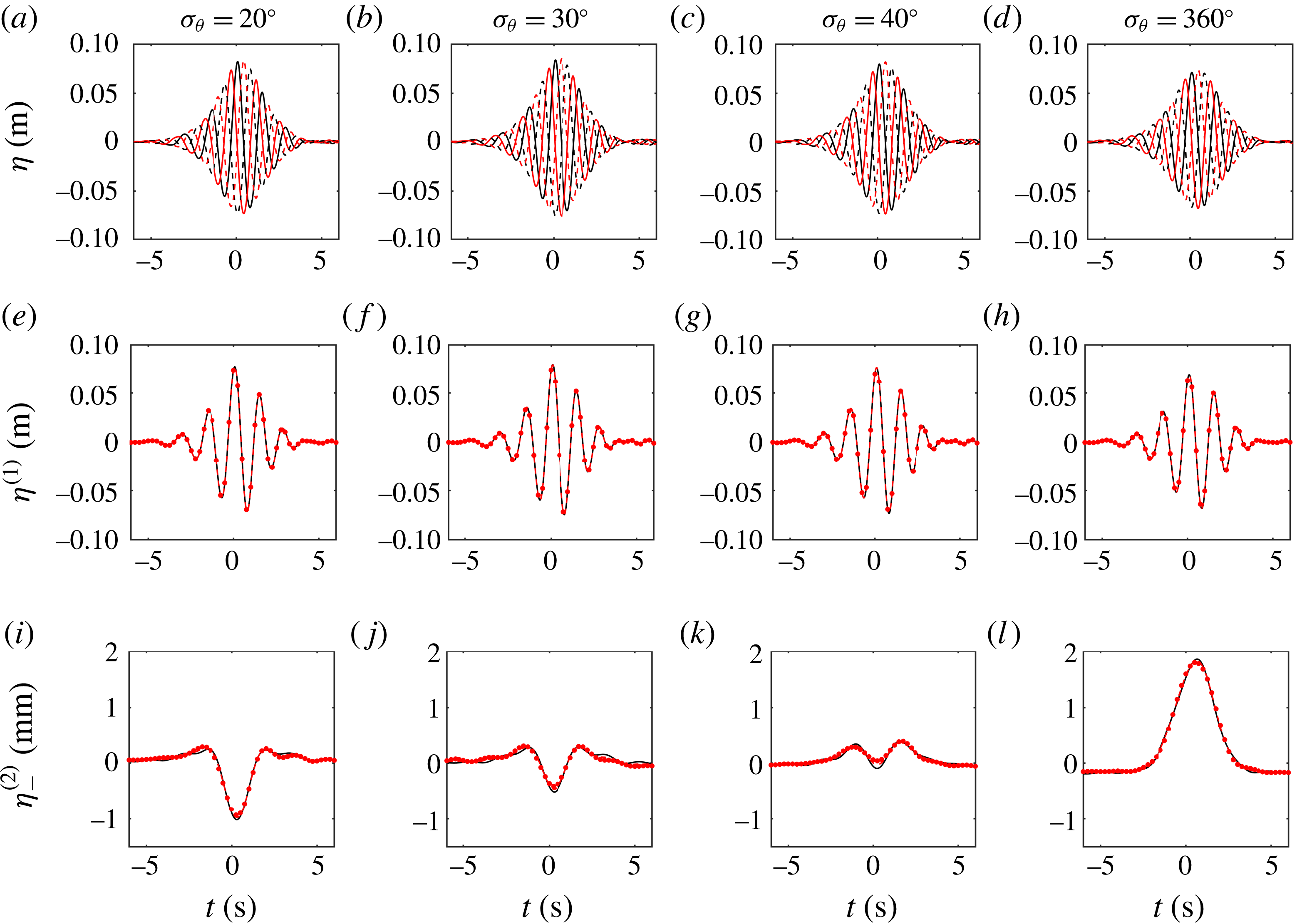
Figure 17. Results of four-phase harmonic extraction for degrees of spreading $\unicode[STIX]{x1D70E}_{\unicode[STIX]{x1D703}}=20,30,40,360^{\circ }$
: measured time series
$\unicode[STIX]{x1D70E}_{\unicode[STIX]{x1D703}}=20,30,40,360^{\circ }$
: measured time series $\unicode[STIX]{x1D702}_{0}$
(black line),
$\unicode[STIX]{x1D702}_{0}$
(black line), $\unicode[STIX]{x1D702}_{90}$
(red line),
$\unicode[STIX]{x1D702}_{90}$
(red line), $\unicode[STIX]{x1D702}_{180}$
(black dashed line) and
$\unicode[STIX]{x1D702}_{180}$
(black dashed line) and $\unicode[STIX]{x1D702}_{270}$
(red dashed line) at the central probe (
$\unicode[STIX]{x1D702}_{270}$
(red dashed line) at the central probe ( $x=0$
,
$x=0$
, $y=0$
) (a–d); extracted linear waves
$y=0$
) (a–d); extracted linear waves $\unicode[STIX]{x1D702}^{(1)}$
(e–h); extracted wave-averaged free surface
$\unicode[STIX]{x1D702}^{(1)}$
(e–h); extracted wave-averaged free surface $\unicode[STIX]{x1D702}_{-}^{(2)}$
(i–j). The black lines denote results obtained from the two-phase method and the red dots those from the four-phase method.
$\unicode[STIX]{x1D702}_{-}^{(2)}$
(i–j). The black lines denote results obtained from the two-phase method and the red dots those from the four-phase method.
By repeating experiments at two further phase shifts of 90 and $270^{\circ }$
, four-phase extraction allows for the following separation of harmonics (Fitzgerald et al.
Reference Fitzgerald, Taylor, Eatock Taylor, Grice and Zang2014):
$270^{\circ }$
, four-phase extraction allows for the following separation of harmonics (Fitzgerald et al.
Reference Fitzgerald, Taylor, Eatock Taylor, Grice and Zang2014):
 $$\begin{eqnarray}\displaystyle & \displaystyle \frac{\unicode[STIX]{x1D702}_{0}-\tilde{\unicode[STIX]{x1D702}}_{90}-\unicode[STIX]{x1D702}_{180}+\tilde{\unicode[STIX]{x1D702}}_{270}}{4}=\unicode[STIX]{x1D702}^{(1)}+\unicode[STIX]{x1D702}^{(3,1)}, & \displaystyle\end{eqnarray}$$
 $$\begin{eqnarray}\displaystyle & \displaystyle \frac{\unicode[STIX]{x1D702}_{0}-\unicode[STIX]{x1D702}_{90}+\unicode[STIX]{x1D702}_{180}-\unicode[STIX]{x1D702}_{270}}{4}=\unicode[STIX]{x1D702}^{(2,2)}+\unicode[STIX]{x1D702}^{(4,2)}, & \displaystyle\end{eqnarray}$$
 $$\begin{eqnarray}\displaystyle & \displaystyle \frac{\unicode[STIX]{x1D702}_{0}+\tilde{\unicode[STIX]{x1D702}}_{90}-\unicode[STIX]{x1D702}_{180}-\tilde{\unicode[STIX]{x1D702}}_{270}}{4}=\unicode[STIX]{x1D702}^{(3,3)}, & \displaystyle\end{eqnarray}$$
 $$\begin{eqnarray}\displaystyle & \displaystyle \frac{\unicode[STIX]{x1D702}_{0}+\unicode[STIX]{x1D702}_{90}+\unicode[STIX]{x1D702}_{180}+\unicode[STIX]{x1D702}_{270}}{4}=\unicode[STIX]{x1D702}^{(2,0)}+\unicode[STIX]{x1D702}^{(4,0)}+\unicode[STIX]{x1D702}^{(4,4)}, & \displaystyle\end{eqnarray}$$
where the tilde denotes a Hilbert transform. Second-order sum and difference terms can now be separated without any filtering. To assess both two- and four-phase methods, tests A.3–4 and A.13 are carried out with four phase shifts, as shown in figure 17(a–d). The linear and wave-averaged surface elevations extracted using both methods are compared in (e)–(h) and (i)–(l) respectively. The results generated by both methods compare very well. Figure 18 displays (log-scaled) amplitude spectra of the extracted harmonic components. Over the range of $0{-}0.5\unicode[STIX]{x1D714}_{0}$
, the sum and difference terms are well separated. Hence, both methods produce similar estimates of the wave-averaged surface elevation.
$0{-}0.5\unicode[STIX]{x1D714}_{0}$
, the sum and difference terms are well separated. Hence, both methods produce similar estimates of the wave-averaged surface elevation.

Figure 18. Amplitude spectra of extracted harmonic components produced using two- and four-phase extraction methods: two-phase results (black lines) and four-phase results (red lines). The different panels correspond to increasing degrees of input directional spreading $\unicode[STIX]{x1D70E}_{\unicode[STIX]{x1D703}}=20,30,40,360^{\circ }$
.
$\unicode[STIX]{x1D70E}_{\unicode[STIX]{x1D703}}=20,30,40,360^{\circ }$
.
Appendix C. Measurement error and repeatability
C.1 Residual tank motion (error measure I)
In order to capture the effect of waves that are not fully absorbed by the wavemakers and remain present in the tank throughout the tests, we measure the variation in the surface elevation after the 10 min of settling time between experiments. Specifically, we define $\unicode[STIX]{x0394}\unicode[STIX]{x1D702}_{I}$
as the difference between the maximum and the minimum surface elevation in the 32 s window before tests. In order to assess the effect of this residual tank motion on the error in the wave-averaged free surface, we apply the same low-pass filter to the residual motion.
$\unicode[STIX]{x0394}\unicode[STIX]{x1D702}_{I}$
as the difference between the maximum and the minimum surface elevation in the 32 s window before tests. In order to assess the effect of this residual tank motion on the error in the wave-averaged free surface, we apply the same low-pass filter to the residual motion.
C.2 Repeatability (error measures II and III)
To quantify the repeatability of tests (error measure II), $\unicode[STIX]{x0394}\unicode[STIX]{x1D702}_{II}$
reports two times the standard deviation of the maximum measured wave-averaged surface amplitude
$\unicode[STIX]{x0394}\unicode[STIX]{x1D702}_{II}$
reports two times the standard deviation of the maximum measured wave-averaged surface amplitude $a_{M-}^{(2)}$
across a number of tests that have been repeated two or three times. Similarly, while performing the spatial measurements, only the mean direction of the wave group is varied. The measurements at the central probe that are thus repeated five times can be used to quantify azimuthal imperfection of the wavemakers and gauge location (error measure III). Two times the standard deviation of the measured wave-averaged surface amplitude
$a_{M-}^{(2)}$
across a number of tests that have been repeated two or three times. Similarly, while performing the spatial measurements, only the mean direction of the wave group is varied. The measurements at the central probe that are thus repeated five times can be used to quantify azimuthal imperfection of the wavemakers and gauge location (error measure III). Two times the standard deviation of the measured wave-averaged surface amplitude $a_{M-}^{(2)}$
for these repeat tests is reported as the error in
$a_{M-}^{(2)}$
for these repeat tests is reported as the error in $\unicode[STIX]{x0394}\unicode[STIX]{x1D702}_{III}$
.
$\unicode[STIX]{x0394}\unicode[STIX]{x1D702}_{III}$
.
C.3 Estimation of directional spreading (error measure IV)
We estimate the error in the predicted value of the wave-averaged surface amplitude $a_{T-}^{(2)}$
that arises from the estimation of the degree of directional spreading
$a_{T-}^{(2)}$
that arises from the estimation of the degree of directional spreading $\unicode[STIX]{x1D70E}_{\unicode[STIX]{x1D703}}^{\star }$
from the linearized signal. The estimates of
$\unicode[STIX]{x1D70E}_{\unicode[STIX]{x1D703}}^{\star }$
from the linearized signal. The estimates of $\unicode[STIX]{x1D70E}_{\unicode[STIX]{x1D703}}^{\star }$
in tables 2–3 are obtained from (3.7) using all 14 probes. Estimation of
$\unicode[STIX]{x1D70E}_{\unicode[STIX]{x1D703}}^{\star }$
in tables 2–3 are obtained from (3.7) using all 14 probes. Estimation of $\unicode[STIX]{x1D70E}_{\unicode[STIX]{x1D703}}^{\star }$
using fewer than 14 probes allows for multiple estimates of
$\unicode[STIX]{x1D70E}_{\unicode[STIX]{x1D703}}^{\star }$
using fewer than 14 probes allows for multiple estimates of $\unicode[STIX]{x1D70E}_{\unicode[STIX]{x1D703}}^{\star }$
using different combinations of probes. Here, we use combinations of seven of the 14 probes (excluding the central probe). This allows for 1716 (
$\unicode[STIX]{x1D70E}_{\unicode[STIX]{x1D703}}^{\star }$
using different combinations of probes. Here, we use combinations of seven of the 14 probes (excluding the central probe). This allows for 1716 ( $=13!/(7!6!)$
) estimates of
$=13!/(7!6!)$
) estimates of $\unicode[STIX]{x1D70E}_{\unicode[STIX]{x1D703}}^{\star }$
, from which we can compute a standard deviation
$\unicode[STIX]{x1D70E}_{\unicode[STIX]{x1D703}}^{\star }$
, from which we can compute a standard deviation $\unicode[STIX]{x0394}\unicode[STIX]{x1D70E}_{\unicode[STIX]{x1D703}}^{\star }$
. To avoid the time-consuming computation of the wave-averaged free-surface amplitude
$\unicode[STIX]{x0394}\unicode[STIX]{x1D70E}_{\unicode[STIX]{x1D703}}^{\star }$
. To avoid the time-consuming computation of the wave-averaged free-surface amplitude $a_{T-}^{(2)}$
for all estimates of
$a_{T-}^{(2)}$
for all estimates of $\unicode[STIX]{x1D70E}_{\unicode[STIX]{x1D703}}^{\star }$
, we compute upper and lower bounds of
$\unicode[STIX]{x1D70E}_{\unicode[STIX]{x1D703}}^{\star }$
, we compute upper and lower bounds of $a_{T-}^{(2)}$
using
$a_{T-}^{(2)}$
using $\unicode[STIX]{x1D70E}_{\unicode[STIX]{x1D703}}^{\star }-2\unicode[STIX]{x0394}\unicode[STIX]{x1D70E}_{\unicode[STIX]{x1D703}}^{\star }$
and
$\unicode[STIX]{x1D70E}_{\unicode[STIX]{x1D703}}^{\star }-2\unicode[STIX]{x0394}\unicode[STIX]{x1D70E}_{\unicode[STIX]{x1D703}}^{\star }$
and $\unicode[STIX]{x1D70E}_{\unicode[STIX]{x1D703}}^{\star }+2\unicode[STIX]{x0394}\unicode[STIX]{x1D70E}_{\unicode[STIX]{x1D703}}^{\star }$
and report the average difference with the mean as our error measure
$\unicode[STIX]{x1D70E}_{\unicode[STIX]{x1D703}}^{\star }+2\unicode[STIX]{x0394}\unicode[STIX]{x1D70E}_{\unicode[STIX]{x1D703}}^{\star }$
and report the average difference with the mean as our error measure $\unicode[STIX]{x0394}\unicode[STIX]{x1D702}_{IV}$
. It should be noted that the means of the resampled spreading estimates agree with the value obtained using all 14 probes, demonstrating that our estimator (3.7) is unbiased.
$\unicode[STIX]{x0394}\unicode[STIX]{x1D702}_{IV}$
. It should be noted that the means of the resampled spreading estimates agree with the value obtained using all 14 probes, demonstrating that our estimator (3.7) is unbiased.

Figure 19. Measured time series $\unicode[STIX]{x1D702}$
at the central probe (
$\unicode[STIX]{x1D702}$
at the central probe ( $x=0$
,
$x=0$
, $y=0$
) for the spreading tests (category A), showing crest-focused groups
$y=0$
) for the spreading tests (category A), showing crest-focused groups $\unicode[STIX]{x1D702}_{0}$
(black lines) and trough-focused groups
$\unicode[STIX]{x1D702}_{0}$
(black lines) and trough-focused groups $\unicode[STIX]{x1D702}_{180}$
(red dashed lines) for an input amplitude of
$\unicode[STIX]{x1D702}_{180}$
(red dashed lines) for an input amplitude of $a_{0}=0.1~\text{m}$
. The different panels correspond to increasing degrees of input spreading
$a_{0}=0.1~\text{m}$
. The different panels correspond to increasing degrees of input spreading $\unicode[STIX]{x1D70E}_{\unicode[STIX]{x1D703}}=0$
–
$\unicode[STIX]{x1D70E}_{\unicode[STIX]{x1D703}}=0$
– $180^{\circ }$
, with estimated values
$180^{\circ }$
, with estimated values $\unicode[STIX]{x1D70E}_{\unicode[STIX]{x1D703}}^{\star }$
given in the labels.
$\unicode[STIX]{x1D70E}_{\unicode[STIX]{x1D703}}^{\star }$
given in the labels.

Figure 20. Measured time series $\unicode[STIX]{x1D702}$
at the central probe (
$\unicode[STIX]{x1D702}$
at the central probe ( $x=0$
,
$x=0$
, $y=0$
) for the spreading tests (category A), showing crest-focused groups
$y=0$
) for the spreading tests (category A), showing crest-focused groups $\unicode[STIX]{x1D702}_{0}$
(black lines) and trough-focused groups
$\unicode[STIX]{x1D702}_{0}$
(black lines) and trough-focused groups $\unicode[STIX]{x1D702}_{180}$
(red dashed lines) for an input amplitude of
$\unicode[STIX]{x1D702}_{180}$
(red dashed lines) for an input amplitude of $a_{0}=0.15~\text{m}$
. The different panels correspond to increasing degrees of input spreading
$a_{0}=0.15~\text{m}$
. The different panels correspond to increasing degrees of input spreading $\unicode[STIX]{x1D70E}_{\unicode[STIX]{x1D703}}=0$
–
$\unicode[STIX]{x1D70E}_{\unicode[STIX]{x1D703}}=0$
– $50^{\circ }$
, with estimated values
$50^{\circ }$
, with estimated values $\unicode[STIX]{x1D70E}_{\unicode[STIX]{x1D703}}^{\star }$
given in the labels.
$\unicode[STIX]{x1D70E}_{\unicode[STIX]{x1D703}}^{\star }$
given in the labels.

Figure 21. Measured time series $\unicode[STIX]{x1D702}$
at the central probe (
$\unicode[STIX]{x1D702}$
at the central probe ( $x=0$
,
$x=0$
, $y=0$
) for the crossing tests (category B), showing crest-focused groups
$y=0$
) for the crossing tests (category B), showing crest-focused groups $\unicode[STIX]{x1D702}_{0}$
(black lines) and trough-focused groups
$\unicode[STIX]{x1D702}_{0}$
(black lines) and trough-focused groups $\unicode[STIX]{x1D702}_{180}$
(red dashed lines) for an input amplitude of
$\unicode[STIX]{x1D702}_{180}$
(red dashed lines) for an input amplitude of $a_{0}=0.1~\text{m}$
, for increasing values of the crossing angle
$a_{0}=0.1~\text{m}$
, for increasing values of the crossing angle $\unicode[STIX]{x0394}\unicode[STIX]{x1D703}=0$
–
$\unicode[STIX]{x0394}\unicode[STIX]{x1D703}=0$
– $180^{\circ }$
and increasing degree of input spreading
$180^{\circ }$
and increasing degree of input spreading $\unicode[STIX]{x1D70E}_{\unicode[STIX]{x1D703}}=10,20,30^{\circ }$
(a–d,e–h,i–l), with estimated values
$\unicode[STIX]{x1D70E}_{\unicode[STIX]{x1D703}}=10,20,30^{\circ }$
(a–d,e–h,i–l), with estimated values $\unicode[STIX]{x1D70E}_{\unicode[STIX]{x1D703}}^{\star }$
given in the labels; (m–p) correspond to increased-amplitude experiments at
$\unicode[STIX]{x1D70E}_{\unicode[STIX]{x1D703}}^{\star }$
given in the labels; (m–p) correspond to increased-amplitude experiments at $a_{0}=0.15~\text{m}$
.
$a_{0}=0.15~\text{m}$
.
C.4 Wave gauge calibration (error measure V)
Finally, the error associated with wave gauge calibration is calculated. The gauges are calibrated by positioning them at known heights in still water and fitting a linear relationship to the resulting measured voltage. Two times the standard deviation of the predicted values of height $z$
is taken as the calibration error
$z$
is taken as the calibration error $\unicode[STIX]{x0394}\unicode[STIX]{x1D702}_{V}$
.
$\unicode[STIX]{x0394}\unicode[STIX]{x1D702}_{V}$
.
Appendix D. Measured time series
The raw data measured at the central probe for the spreading tests (category A) are presented in figures 19 and 20 and for the crossing tests (category B) in figure 21. Both crest- and trough-focused repeat experiments are shown. In general, the experiments exhibit good focusing, with maxima occurring at $t=0$
, and display horizontal symmetry. However, for the long-crested increased-amplitude wave groups in figure 20, the groups exhibit horizontal asymmetry. Here, the dispersion of the free waves is affected by cubic nonlinearity, shifting the location at which the waves focus, as also observed by Taklo et al. (Reference Taklo, Trulsen, Krogstad and Borge2017), among others. As discussed in § 3.3, this will not affect the extraction of the measured wave-averaged surface elevation, but will introduce a phase shift.
$t=0$
, and display horizontal symmetry. However, for the long-crested increased-amplitude wave groups in figure 20, the groups exhibit horizontal asymmetry. Here, the dispersion of the free waves is affected by cubic nonlinearity, shifting the location at which the waves focus, as also observed by Taklo et al. (Reference Taklo, Trulsen, Krogstad and Borge2017), among others. As discussed in § 3.3, this will not affect the extraction of the measured wave-averaged surface elevation, but will introduce a phase shift.
Appendix E. Frequency-sum components
As well as the wave-averaged surface elevation, the second-order frequency-sum components $\unicode[STIX]{x1D702}_{+}^{(2)}$
corresponding to the linear signal (2.20) may be calculated (Dalzell Reference Dalzell1999),
$\unicode[STIX]{x1D702}_{+}^{(2)}$
corresponding to the linear signal (2.20) may be calculated (Dalzell Reference Dalzell1999),
 $$\begin{eqnarray}\unicode[STIX]{x1D702}_{+}^{(2)}=\mathop{\sum }_{n=1}^{N_{\unicode[STIX]{x1D714}}}\mathop{\sum }_{m=1}^{N_{\unicode[STIX]{x1D714}}}\mathop{\sum }_{i=1}^{N_{\unicode[STIX]{x1D703}}}\mathop{\sum }_{j=1}^{N_{\unicode[STIX]{x1D703}}}\unicode[STIX]{x1D6FA}(\unicode[STIX]{x1D703}_{i})\unicode[STIX]{x1D6FA}(\unicode[STIX]{x1D703}_{j})\hat{\unicode[STIX]{x1D702}}_{n}\hat{\unicode[STIX]{x1D702}}_{m}B^{+}(\boldsymbol{k}_{n,i},\boldsymbol{k}_{m,j},\unicode[STIX]{x1D714}_{n},\unicode[STIX]{x1D714}_{m},d)\cos (\unicode[STIX]{x1D711}_{n,i}+\unicode[STIX]{x1D711}_{m,j}),\end{eqnarray}$$
where the interaction kernel $B^{+}$
is given in appendix A.
$B^{+}$
is given in appendix A.

Figure 22. The amplitude of the second-order frequency-sum components at the central probe ( $x=0$
,
$x=0$
, $y=0$
) for the spreading tests (category A). (a) The measured amplitude
$y=0$
) for the spreading tests (category A). (a) The measured amplitude $a_{M+}^{(2)}$
as a function of the theoretical prediction
$a_{M+}^{(2)}$
as a function of the theoretical prediction $a_{T+}^{(2)}$
, with error bars shown in grey (see § 3.6 and appendix C for details), and (b) the measured amplitude
$a_{T+}^{(2)}$
, with error bars shown in grey (see § 3.6 and appendix C for details), and (b) the measured amplitude $a_{M+}^{(2)}$
as a function of the estimated degree of spreading
$a_{M+}^{(2)}$
as a function of the estimated degree of spreading $\unicode[STIX]{x1D70E}_{\unicode[STIX]{x1D703}}^{\star }$
.
$\unicode[STIX]{x1D70E}_{\unicode[STIX]{x1D703}}^{\star }$
.

Figure 23. The amplitude of the second-order frequency-sum components at the central probe ( $x=0$
,
$x=0$
, $y=0$
) for the crossing tests (category B). (a) The measured amplitude
$y=0$
) for the crossing tests (category B). (a) The measured amplitude $a_{M+}^{(2)}$
as a function of the theoretical prediction
$a_{M+}^{(2)}$
as a function of the theoretical prediction $a_{T+}^{(2)}$
, with error bars shown in grey (see § 3.6 and appendix C for details), and (b) the measured amplitude
$a_{T+}^{(2)}$
, with error bars shown in grey (see § 3.6 and appendix C for details), and (b) the measured amplitude $a_{M+}^{(2)}$
as a function of the crossing angle
$a_{M+}^{(2)}$
as a function of the crossing angle $\unicode[STIX]{x0394}\unicode[STIX]{x1D703}$
.
$\unicode[STIX]{x0394}\unicode[STIX]{x1D703}$
.
For a single wave group, figure 22 compares the measured amplitude of the frequency-sum components $a_{+}^{(2)}$
with those predicted for a single Gaussian wave group (category A) as a function of the spreading. Here,
$a_{+}^{(2)}$
with those predicted for a single Gaussian wave group (category A) as a function of the spreading. Here, $a_{+}^{(2)}$
is calculated using the wave envelope in order to circumvent the phase-sensitive nature of these high-frequency waves. As the frequency-sum components are composed of high-frequency waves, the location of the maximum is more sensitive to the phase. At low values of spreading, the sum waves are larger than expected for a Gaussian wavepacket, which could be the result of unabsorbed reflections or a non-Gaussian spectral tail.
$a_{+}^{(2)}$
is calculated using the wave envelope in order to circumvent the phase-sensitive nature of these high-frequency waves. As the frequency-sum components are composed of high-frequency waves, the location of the maximum is more sensitive to the phase. At low values of spreading, the sum waves are larger than expected for a Gaussian wavepacket, which could be the result of unabsorbed reflections or a non-Gaussian spectral tail.
For two crossing groups, figure 23 shows the measured amplitude of the frequency-sum components $a_{+}^{(2)}$
as a function of the crossing angle (category B). As with the spreading tests, the measured values
$a_{+}^{(2)}$
as a function of the crossing angle (category B). As with the spreading tests, the measured values $a_{M+}^{(2)}$
are larger than predicted for Gaussian wavepackets at low crossing angles only. For larger crossing angles, the theory and the experiments agree well. Panel (a) compares the predicted amplitudes of the frequency-sum components
$a_{M+}^{(2)}$
are larger than predicted for Gaussian wavepackets at low crossing angles only. For larger crossing angles, the theory and the experiments agree well. Panel (a) compares the predicted amplitudes of the frequency-sum components $a_{T+}^{(2)}$
with the measured ones
$a_{T+}^{(2)}$
with the measured ones $a_{M+}^{(2)}$
, showing good agreement.
$a_{M+}^{(2)}$
, showing good agreement.


 Open access