


I. INTRODUCTION
Nanoporous materials made by dealloying present themselves as a stochastic open-cell ligament networks at nanoscale with solid volume fractions in between 0.25 and 0.50.Reference Li and Sieradzki1–Reference Hu, Ziehmer, Wang and Lilleodden4 High yield strength to phase volume ratio, large specific surface area, and electrocatalytic performance are among towering features popularizing their use in applications such as catalysts, sensors, optical-active materials, mechanical actuators, fuel cell and microbalance electrodes, and coating for medical devices.Reference Erlebacher, Aziz, Karma, Dimitrov and Sieradzki2,Reference Weissmüller, Viswanath, Kramer, Zimmer, Würschum and Gleiter5,Reference Chen, Chu, Yi, McNulty, Shen, Voorhees and Dunand6 Upon mechanical loading, a bending-dominated load transmission occurs among interconnected ligaments.Reference Griffiths, Bargmann and Reddy7 Thus, the Gibson–Ashby scaling relationReference Gibson and Ashby8 is frequently used with reference to their mechanical behavior. However, this leads to more than an order of magnitude over-prediction of the Young’s modulus especially with smaller solid volume fractions.Reference Hu, Ziehmer, Wang and Lilleodden4,Reference Huber, Viswanath, Mameka, Markmann and Weissmüller9–Reference Mangipudi, Epler and Volkert15
This prediction gap is bridged by devising 3D finite element (FE)-based micromechanical analyses of representative volumes, see, e.g., Refs. Reference Hu, Ziehmer, Wang and Lilleodden4 and Reference Soyarslan, Bargmann, Pradas and Weissmüller13. In Ref. Reference Hu, Ziehmer, Wang and Lilleodden4, a representative volume element (RVE) is formed through 3D tomographic reconstructions using a dual-beam focused ion beam (FIB) and scanning electron microscopy (SEM). The identified phase domain is then discretized with quadratic tetrahedral FEs and used in simulations of compressive loading. In Ref. Reference Soyarslan, Bargmann, Pradas and Weissmüller13, a new scaling relation, as a modification of that suggested in Ref. Reference Roberts and Garboczi16, is proposed based on the simulation results devising voxel-based FE discretizations of a stochastic random composition field representing the early stages of spinodal decomposition as conceived in Ref. Reference Cahn17. However, these models require a notably large amount of solid FEs and degrees of freedom which demand high computational power.
To remedy this high computational source demand, however, regarding simulation of bone tissue for which classically voxel-based FE simulations were conducted, see, e.g., Refs. Reference Hollister, Brennan and Kikuchi18–Reference van Rietbergen, Odgaard, Kabel and Huiskes20, researchers proposed the use of beam-FE or beam-shell-FE models.Reference Pothuaud, van Rietbergen, Charlot, Ozhinsky and Majumdar21–Reference Vanderoost, Jaecques, der Perre, Boonen, D’hooge, Lauriks and van Lenthe24 A 3D-line skeleton graph analysis technique was used in Ref. Reference Pothuaud, van Rietbergen, Charlot, Ozhinsky and Majumdar21 to describe the internal structure of the trabecular bone, and a network of straight beam elements were utilized for determining the stiffnesses. In these alternative studies, the authors obtained satisfactory agreement with those computed from voxel-based FE models having solid elements. Moreover, significant reductions in the computational costs pertaining to time and memory are reported. In the context of nanoporous gold, an efficient FE beam-based modeling approach relying on skeletonization has first been reported in Ref. Reference Bargmann, Klusemann, Markmann, Schnabel, Schneider, Soyarslan and Wilmers25. In Ref. Reference Richert and Huber26, a similar idea based on 3D focused ion beam-SEM tomography data is pursued.
In the current study, we revisit Cahn’s algorithm (Ref. Reference Cahn17, see also Ref. Reference Soyarslan, Bargmann, Pradas and Weissmüller13) to generate a periodic skeletonization-based efficient beam-FE model representing 3D stochastic bicontinuous microstructures. The beam-FE model is derived from homotopic medial axis skeletonization of the spinodal-like stochastic microstructures generated by a convenient and fast numerical algorithm computing a leveled periodic random field composed of superposition of standing sinusoidal waves of fixed wave length. For the possible influence of shear strains, especially for beams having thicker cross sections, Timoshenko beam theory is utilized. For the diameter of the assumed circular cross sections, a 3D local thickness field computation is used. Thus, in terms of providing an accurate thickness distribution assignment and by carrying the native topological features of the phase field, the presented periodic skeletonization-based microstructure generation method proves superior to the regular or disordered beam network approaches relying on perfect and randomized diamond-cubic unit cellsReference Huber, Viswanath, Mameka, Markmann and Weissmüller9,Reference Roschning and Huber10,Reference Stavans27,Reference Glazier and Weaire28 or Voronoi or Laguerre tessellations.Reference Roberts and Garboczi29–Reference Redenbach, Shklyar and Andrä32 For an extended review of relevant microstructure generation methods, the reader is referred to Ref. Reference Bargmann, Klusemann, Markmann, Schnabel, Schneider, Soyarslan and Wilmers25 and the references therein. To mimic the stiffening with agglomeration of the mass in junctions, an increased Young’s modulus is assigned to the elements within the junction zone through a radially varying stiffness scaling factor. While doing so, the effective Young’s modulus, effective Poisson’s ratio, and effective universal anisotropy index values are computed for the developed microstructures.
II. STOCHASTIC MICROSTRUCTURE GENERATION
Computational mechanics of composites relies on computational micro-to-macro transition.Reference Miehe and Koch33,Reference McBride, Mergheim, Javili, Steinmann and Bargmann34 Figure 1 depicts a composite through the notion of a continuum with microstructure for a porous material and possible discretization strategies for numerical simulation. Here,  ${}^{\rm{M}}{\cal B} \subset {{\cal R}^3}$ represents the homogenized macrocontinuum. Each material point ${}^{\rm{M}}{\bi{x}} \in {}^{\rm{M}}{\cal B}$ at the macroscale encapsulates a so-called representative volume ${\cal V} \subset {{\cal R}^3}$ composed of a solid and pore phase denoted by ${\cal B} \subset {{\cal R}^3}$ and ${\cal P} \subset {{\cal R}^3}$, respectively. The averages of the microscopic stress and strain fields over the RVE centered at a material point give the macroscopic stress and strain fields at the same point, as resultants of a boundary value problem (at the microscale) once the condition of separation of scales holds with ${}^\mu {\cal L} \ll {}^{{\rm{RVE}}}{\cal L} \ll {}^{\rm{M}}{\cal L}$Reference Zaoui35–Reference Torquato37 where the characteristic size of a microstructural feature (e.g., ligament diameter) is denoted by ${}^\mu {\cal L}$. The averaging process, once computationally realized, could devise different discretization strategies, see, e.g., Fig. 1.
Each material point  $^{\rm{M}}{\bi{x}} \in {\;^{\rm{M}}}{\cal B}$ in macrocontinuum ${}^{\rm{M}}{\cal B}$ corresponds to a microstructure ${\cal B}$ of the representative volume ${\cal V}$ whose effective behavior is representative of that of the material as a whole. Here, ${}^{\rm{M}}{\cal L}$ denotes the characteristic size of the body at macroscale or the length scale associated with the fluctuations of the applied mechanical loading. ${}^{{\rm{RVE}}}{\cal L}$ is the RVE size. Computationally, different discretization strategies are possible in the representation of the domain, e.g., a voxel-FE or beam-FE model, as used in the current work.

A. Periodic random field
Let x, N, qi, and φi denote the position vector, the number of waves, wave direction, and wave phase of the ith wave, respectively. Let a constant wave number q i = |qi| = q 0 with uniformly distributed wave directions over the solid angle 4π and wave phases uniformly distributed on [0, 2π). In view of these definitions, we consider a random field f(r) generated by superimposing standing sinusoidal waves of fixed wave length and amplitude but random direction and phaseReference Cahn17:
 $$f\left( {\bi{x}} \right) = {\left[ {{2 \over N}} \right]^{{1 / 2}}}\sum\limits_{i = 1}^N {\cos \left( {{{\bi{q}}_i} \cdot {\bi{x}} + {\varphi _i}} \right)} \quad .$$
Given the random function (1), the different phases of the system are defined via a level cut ξ:
 $${\bi{x}} \in {\cal B}\quad {\rm{if}}\quad f\left( {\bi{x}} \right) \lt \xi \quad ,$$
 $${\bi{x}} \in \partial {\cal B}\quad {\rm{if}}\quad f\left( {\bi{x}} \right) = \xi \quad ,$$
 $${\bi{x}} \in {\cal P}\quad {\rm{if}}\quad f\left( {\bi{x}} \right) > \xi \quad .$$
 Letting |{•}| denote the volume contained in {•}, the volumes fractions of the solid and pores are represented by  ${\phi _{\cal B}} = {{\left| {\cal B} \right|} / {\left| {\cal V} \right|}}$ and ${\phi _{\cal P}} = {{\left| {\cal P} \right|} / {\left| {\cal V} \right|}}$, respectively, with $\left| {\cal V} \right| = \left| {\cal B} \right| + \left| {\cal P} \right|$ and thus ${\phi _{\cal B}} + {\phi _{\cal P}} = 1$. Under the given conditions, $f\left( {\bi{x}} \right)$ is a Gaussian random field with 〈f〉 = 0, 〈f 2〉 = 1. Letting erf−1(x) denote the inverse error function, this allows linking the phase volume fraction ${\phi _{\cal B}}$ to the level cut ξ by
 $$\xi \left( {{\phi _{\cal B}}} \right) = {2^{{1 / 2}}}{\rm{er}}{{\rm{f}}^{ - 1}}\left( {2{\phi _{\cal B}} - 1} \right)\quad .$$
Within a selected finite domain size, the fields generated using Eq. (1) are generally not periodic. However, translational periodicity of f with lattice vectors of magnitude a can be achieved by making use of waves with qi of Eq. (1) be of the form
 $${\bi{q}} = {{2\pi } \over a}\left( {h,k,l} \right)\quad ,$$
where the Miller indices h, k, and l are integers amounting to H = [h 2 + k 2 + l 2]1/2 hence constant |q| = q 0 = 2πH/a. Aiming at a high multiplicity, as well as a sufficient number of wavelengths represented within a, the considered microstructures in this work derives from random fields with H = 1461/2 with 〈0 5 11〉-, 〈1 1 12〉-, 〈1 8 9〉-, 〈3 4 11〉-, and 〈4 7 9〉-type vectors, leading to N = 96 independent directions. For further details on the generation and the elastic and topological properties of these microstructures, the reader is referred to Soyarslan et al.Reference Soyarslan, Bargmann, Pradas and Weissmüller13
B. Generation of periodic beam-FE model microstructures
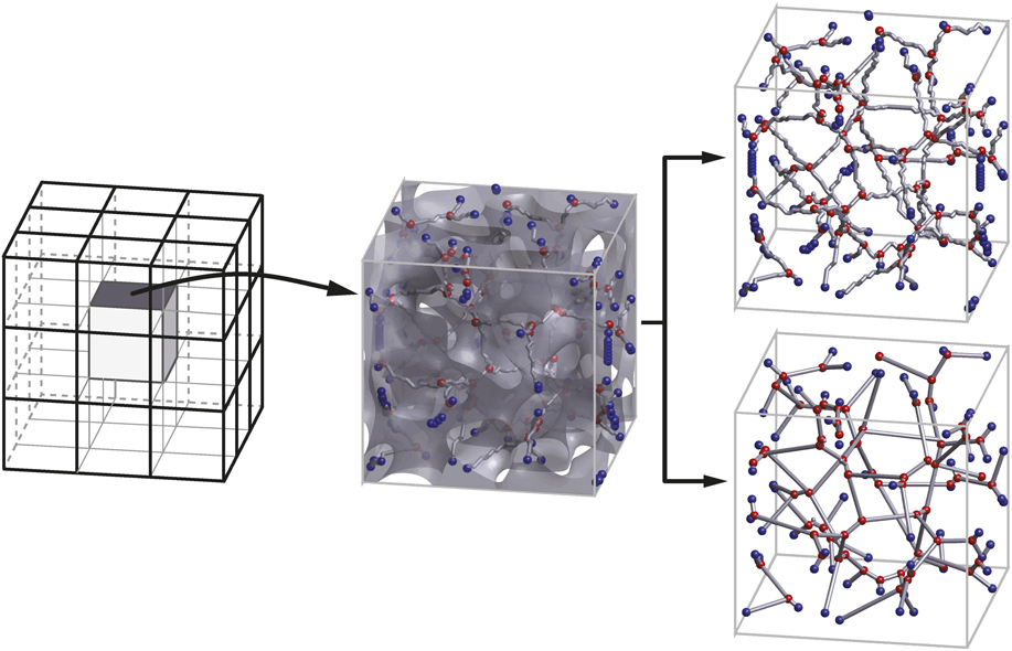
Unlike other studies,Reference Huber, Viswanath, Mameka, Markmann and Weissmüller9,Reference Roschning and Huber10 which use regular or disordered diamond-cubic unit cells in the development of beam networks, generation of the more realistic beam-FE model in the current study requires skeletonization of the underlying random periodic field. To this end, we use a modified version of MATLAB script Skeleton3D.Reference Kerschnitzki, Kollmannsberger, Burghammer, Duda, Weinkamer, Wagermaier and Fratzl38 As an input, Skeleton3D uses a binary image sequence, i.e., the voxel representation of the 3D phase distribution within a finite domain size. One-voxel-thick medial axis skeleton, homotopic to the original image, is created by a connectivity preserving thinning algorithm which relies on an iterative removal of the surface voxels of the binarized image belonging to the periodic field. While doing so, skeleton pruning is applied where redundant branches shorter than a threshold length are removed. The voxels making up the skeleton are then linked by beam FEs with circular cross sections. This makes each skeleton voxel an FE node. A node merging more than two ligaments is referred to as a junction. In the simplified beam network models, the junctions connected by ligaments are merged by straight links composed of one or many beam elements. Although voxelizing a 3D cubic cell with edge length of lattice parameter a in view of Eq. (4) assures the periodicity of the voxelization, due to boundary effects, periodicity of the skeletonization is not guaranteed. To remedy this, we consider a cubic domain size of 3a × 3a × 3a over which the random field is computed and voxelization is realized. After the application of the skeletonization, the skeleton of the central cubic cell with size a × a × a is clipped out, as depicted in Fig. 2.
Periodicity of the generated beam-FE model is provided by making use of topology conserving medial axis skeletonization of the voxelization of the random periodic field over a 3a × 3a × 3a sized domain. Then, the one-voxel-thick skeleton of a × a × a central cubic cell is clipped out. The voxels making up the skeleton are then linked by ligaments to each of which a circular beam section is assigned (right-top). This makes each skeleton voxel a FE node. A node merging more than two ligaments is referred to as junction which is depicted by red spheres. Blue spheres denote periodically located nodes at the periodic volume element face of size a × a × a. In the simplified beam network models, the junctions connected by ligaments are merged by straight links composed of one or many beam elements (right-bottom). In this process, all junction and periodically located node positions are preserved.
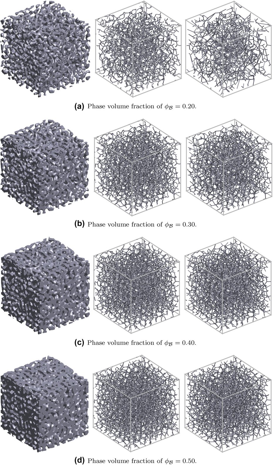
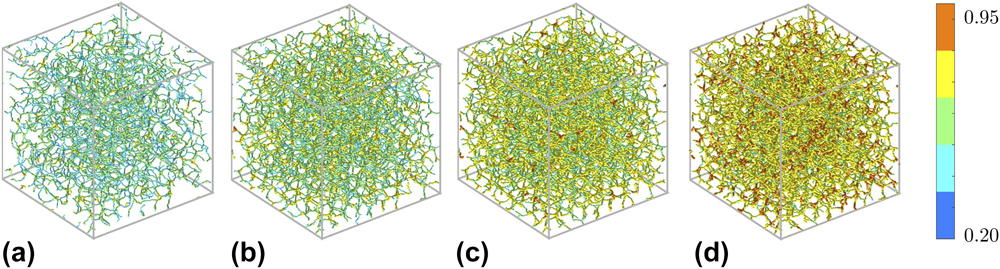
In this work, 128 × 128 × 128 voxelization of the random field realizations are considered over a single unit cell of size a. Figure 3 demonstrates the phase distribution for microstructures with phase volume fractions  ${\phi _{\cal B}}$ ranging from 0.20 to 0.50 and the corresponding two beam-FE model generated by making use of the developed periodic skeletonization procedure. The density and connectivity of the ligaments are higher for the volume fraction of 0.5 if compared to those of 0.2.
Generated (left) 3D periodic phase field, (b) one-to-one periodic skeleton based beam-FE model, and (c) simplified periodic beam network for the single level cut method for solid volume fractions of (a) 0.20, (b) 0.30, (c) 0.40, and (d) 0.50. The number of beam elements for corresponding discretizations are (a) 18,317 and 3674, (b) 26,786 and 8166, (c) 31,989 and 11,479, and (d) 34,351 and 12,716.
C. Local thickness distribution
A complete geometrical description of the discretization of the domain with beam FEs having circular cross sections is not possible without identification of the radii of the cross sections. To this end, we follow a path similar to the steps in Ref. Reference Badwe, Chen and Sieradzki39 where the distribution of local dimensions of the ligaments of nanoporous gold is recovered from the skeletonized scanning electron micrographs and Euclidean distance fields. The ligament diameter at an arbitrary node of the beam network is retrieved from the local thickness field qualified using the plugin BoneJReference Hildebrand and Rüegsegger40–Reference Dougherty and Kunzelmann42 of the open-source image analysis platform Fiji.Reference Schindelin, Arganda-Carreras, Frise, Kaynig, Longair, Pietzsch, Preibisch, Rueden, Saalfeld, Schmid, Tinevez, White, Hartenstein, Eliceiri, Tomancak and Cardona43 In this method, the local thickness D(p) at point  ${\bi{p}} \in {\cal B}$ is defined by the diameter of the largest sphere inside the structure which contains the point p,Reference Hildebrand and Rüegsegger40 i.e.,
 $$D\left( {\bi{p}} \right) = 2 \times \max \left( {\left\{ {{\it{r}}{\rm{:}}\;{\bi{p}} \in {\rm{sph}}\left( {{\bi{x}},{\it{r}}} \right) \subseteq {\cal B},\;{\bi{x}} \in {\cal B}} \right\}} \right)\quad .$$
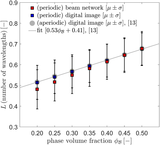
Figure 4 demonstrates the local thickness distribution of the periodic beam-FE model produced for phase volume fractions of 0.20, 0.30, 0.40, and 0.50. As anticipated, junctions acquire larger diameters. Figure 5 shows the distribution of the mean ligament diameter for the beam-FE model as a function of phase volume fraction. It is seen that, although the mean ligament diameter increases with increased phase volume fraction, the change in the standard deviation seems to be marginal. Figure 5 also shows that there is a good agreement between the periodic beam-FE model computations with the voxel-FE computations presented in Ref. Reference Soyarslan, Bargmann, Pradas and Weissmüller13.
Local thickness distribution of the generated beam-FE models for (a) 0.20, (b) 0.30, (c) 0.40, and (d) 0.50 phase volume fractions following the method provided in Ref. Reference Badwe, Chen and Sieradzki39 in conjunction with Refs. Reference Hildebrand and Rüegsegger40 and Reference Dougherty and Kunzelmann42. An increase in the ligament diameters with increasing phase volume fraction with junctions acquiring relatively higher thickness in each case is evident. Local thicknesses are given in terms of wave length λ = 2π/q 0 of the random field.
Local thickness distribution for the developed beam-FE models as a function of phase volume fraction computed using the method provided in Ref. Reference Badwe, Chen and Sieradzki39 in conjunction with Refs. Reference Hildebrand and Rüegsegger40 and Reference Dougherty and Kunzelmann42. Data are presented as averages of the means μ (dots) and averages of the standard deviations σ from ligament diameter distribution analysis over 5 random realizations. A comparison with the data from Ref. Reference Soyarslan, Bargmann, Pradas and Weissmüller13 is also provided in which computations over 3D images of 36 wave length size aperiodic microstructures with 512 × 512 × 512 voxel discretization are considered. The results are presented in terms of the wave length λ = 2π/q 0 of the random field. Despite the differences in both domain size of computation and discretization resolution, a good agreement especially with increasing phase volume fraction is observed.
III. ELASTOMECHANICAL CHARACTERIZATION OF PERIODIC BEAM FE MODELS
A. Periodic homogenization and effective mechanical property determination
Let the displacement field at  ${\bi{x}} \in {\cal B}$ at time $t \in {{\cal R}_ + }$ be denoted by ${\bi{u}}{\rm{:}}\;{\cal B} \times {{\cal R}_ + } \to {{\cal R}^3}$ and σ is the Cauchy stress tensor. Omitting dynamic effects and body forces, the microequilibrium is defined via divσ = 0 in ${\cal B}$. In view of linear and infinitesimal elasticity, we use ${\bf{σ}} = ℂ{\rm{:}}{\bf{ε}}$ in ${\cal B}$, where $ℂ$ is the elastic constitutive tensor and ε := sym(d) is the microscopic strain tensor with d = ∇u denoting the displacement gradient. Considering elastic isotropy at the microscale, the definition of $ℂ$ requires only two material constants: the Young’s modulus E and the Poisson’s ratio ν.
The macroscropic response of the composite is identified through an averaged Hooke’s law
 $$^{\rm{M}}{\bf{σ }} = {ℂ^ \star }{{\rm{:}}^{\rm{M}}}{\bf{ε }}\;{\rm{in}}{\;^{\rm{M}}}{\cal B}\quad ,$$
with  ${ℂ^ \star }$, Mσ, and Mε denoting averaged elastic constitutive, stress and strain tensors, respectively. At the macroscale, the composite is not necessarily isotropic. Thus, ${ℂ^ \star }$ has 36 effective constitutive constants where only 21 of them are independent. These constants are determined by computing Mσ〈i〉 for i = 1, …, 6 independent load cases which are fully prescribed in terms of macroscopic strain tensor Mε〈i〉 that is imposed to the RVE by means of a convenient macroscropic displacement gradient Md〈i〉 through four master nodes only. These points correspond to the corners in a cubic RVE and have reference positions x{1} = (0,0,0), x{2}/|x{2}| = (1,0,0), x{3}/|x{3}| = (0,1,0), and x{4}/|x{4}| = (0,0,1). Under applied macroscopic loading i, the displacement vector of control node j is fully prescribed as u{j}〈i〉(t) = Md〈i〉(t)·x{j}.
With  ${{\bi{x}}^ + } \in \partial {{\cal V}^ + }$ and ${{\bi{x}}^ - } \in \partial {{\cal V}^ - }$ denoting two nodes periodically located, the application of 6 independent load cases are conducted under periodic boundary conditions considering periodic displacements u and rotations θ as
 $${{\bi{u}}_{\left\langle i \right\rangle }}\left( {{{\bi{x}}^ + },\;t} \right) - {{\bi{u}}_{\left\langle i \right\rangle }}\left( {{{\bi{x}}^ - },\;t} \right) = {}^{\rm{M}}{{\bi{d}}_{\left\langle i \right\rangle }}\left( t \right) \cdot \left[ {{{\bi{x}}^ + } - {{\bi{x}}^ - }} \right]\quad ,$$
 $${{\bf{θ}} _{\left\langle i \right\rangle }}\left( {{{\bi{x}}^ + },\;t} \right) - {{\bf{θ}} _{\left\langle i \right\rangle }}\left( {{{\bi{x}}^ - },\;t} \right) = {\bf{0}}\quad .$$
With the limitation to geometrically linear analysis, the homogenized stresses are then computed viz.Reference Kouznetsova, Brekelmans and Baaijens44
 $${}^{\rm{M}}{{\bf{σ}} _{\left\langle i \right\rangle }} = {1 \over {\left| {\cal V} \right|}}\sum\limits_{j = 1}^4 {{{\bi{f}}_{\left\{ j \right\}\left\langle i \right\rangle }}} \otimes {{\bi{x}}_{\left\{ j \right\}}}\quad ,$$
where f{j}〈i〉 is the external force applied to control node j during load case i. The symmetry of Mσ〈i〉 is guaranteed for the converged solution which provides the rotational equilibrium of forces f{j}〈i〉.Reference Kouznetsova, Brekelmans and Baaijens44 Once the computational homogenization is completed, the extent of anisotropy in  ${ℂ^ \star }$ may be quantified using the universal anisotropy index A U.Reference Ranganathan and Ostoja-Starzewski45
 $${A^{\rm{U}}} = {{{K_{\rm{V}}}} \over {{K_{\rm{R}}}}} + 5{{{\mu _{\rm{V}}}} \over {{\mu _{\rm{R}}}}} - 6 \ge 0\quad ,$$
where K V, μV, K R, and μR are Voigt and Reuss estimates for the isotropicized single crystal elasticity shear and bulk moduli, respectively. For elastic isotropy, A U = 0 and A U > 0 increase with increasing elastic anisotropy.
B. Treatment of local stiffening in the vicinity of junctions
Consideration of the agglomeration of the mass in junctions is crucial for an accurate identification of the stiffness in bending dominated structures such as the ligament network of nanoporous gold.Reference Huber, Viswanath, Mameka, Markmann and Weissmüller9,Reference Roschning and Huber10,Reference Pia and Delogu46,Reference Liu and Antoniou47 With this mass agglomeration, there occurs a considerable increase in the bending resistance through the increase in the section’s moment of inertia in junction vicinities. In beam-FE models, this cannot be compensated by using the increased local thickness around junctions. The joint stiffening methods for 3D steel framed structures dates back to 1963Reference Monforton and Wu48 and constitute a wide field of research area. For the details of these studies, one may refer to the review paper by Diaz et al.Reference Díaz, Martí, Victoria and Querin49 In the spirit of these studies, a junction zone strategy is devised in this work. Accordingly, an increased Young’s modulus is assigned to the elements within the junction zone through a stiffness scaling factor as summarized in Fig. 6.
Mechanical treatment of the stiffening around junctions with agglomeration of the mass is realized through increasing the Young’s modulus with a scaling factor ω(r). (a) An example junction of a nanoporous material. Here, the transparent gray region bounded by solid black lines represents the solid phase whereas the shaded 3D lines represent the corresponding skeleton. r denotes the radial distance from the junction, whereas R denotes the local thickness computed at the junction. The distribution can be assumed to be constant within the junction zone, i.e., for r < R, as depicted in (b). Another approach may be selection of a nonlinear distribution, e.g., depicted in (c). In this work, approach (b) is used.

IV. RESULTS AND DISCUSSION
A. Model details
In this study, only periodic beam-FE models with one-to-one utilization of the underlying homotopic medial axis skeleton in the absence of any network simplifications, see Fig. 2, are considered. Since periodic structures are concerned, the computed responses are deemed to be effective for each individual realization. Phase volume fractions of 0.20, 0.25, 0.30, 0.40, 0.45, and 0.50 are investigated considering nanoporous gold made by dealloying. Each investigation is supported by five stochastic realizations satisfying H = 1461/2 to collect sufficient statistical information.
All reported results use 384 × 384 × 384 voxelizations having fixed sizes for the periodic skeletonization procedure with the skeleton occupying the central 128 × 128 × 128 voxel region is clipped out for simulations. By this way, we provide a voxel resolution which is identical to the one that is used in voxel-based FE simulation,Reference Soyarslan, Bargmann, Pradas and Weissmüller13 in which the voxel size was determined through mesh convergence analysis.
Notwithstanding with the elastic anisotropy of the gold single crystal, we assume elastic isotropy of the solid phase with  ${E_{\cal B}} = 79$ GPa and ${\nu _{\cal B}} = 0.44$.Reference Davis50 Since the properties exhibited by the surfaces of the bodies are different from those associated with their interiors, in nanosized samples of nanoporous gold, the stored energy in the surfaces can become comparable to that of the bulk. As a consequence, a dramatic elastic stiffness gain is observed in nanoporous metal samples with reduction of the average ligament diameter at sub-micron scale, see, e.g., Refs. Reference Soyarslan, Husser and Bargmann51–Reference Lu, Xie, Li, Huang, Li and Zhou53, and the references therein. In Ref. Reference Lu, Xie, Li, Huang, Li and Zhou53, randomly connected beam-FE networks accounting for surface elasticity theory and constructed using Voronoi tessellations are used. In the context of plasticity, surface and inner grain boundary conditions play a significant role for crystals at small scales through affecting the dislocation activity and thus hardening behavior, see, e.g., Ref. Reference Husser, Soyarslan and Bargmann54. This constitutes another source for size-affected mechanical response which is not considered in conventional continuum mechanics estimates. Following in line with our earlier studies in Ref. Reference Soyarslan, Bargmann, Pradas and Weissmüller13, we leave the size effect beyond the scope of the current study. Since no size dependent constitutive phenomena are considered, the computed mechanical properties are equally valid for any ligament size.
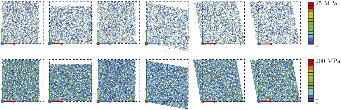
The investigations are realized considering constant stiffness intensity factors of ω(r) ∈ {1, 5, 20, 40} for r < R. Figure 7 demonstrates the von Mises stress distribution among ligaments for 0.20 (top) and 0.50 (bottom) volume fractions for ω(r) = 40. As compared to the 0.20 volume fraction case, over 8-fold higher magnitudes are observed as far as the local stress development in the ligaments of 0.50 volume fraction model is concerned. In both cases, due to random ligament orientations, strong local stress fluctuations are observed. Nevertheless, among the plane strain compression tests and among the simple shear tests conducted in different directions, the statistical distribution of the observed von Mises stress magnitudes over the ligaments are in complete agreement. This signals the isotropy in the macroscropic elastic response of the ligament network.
von Mises stress distributions for the models with 0.20 (top) and 0.50 (bottom) phase volume fractions under six strain-controlled loading conditions with the macroscopically imposed strains of (from left to right) Mε〈1〉 = αe1 ⊗ e1, Mε〈2〉 = αe2 ⊗ e2, Mε〈3〉 = αe3 ⊗ e3, Mε〈4〉 = [α/21/2][e2 ⊗ e3 + e3 ⊗ e2], Mε〈5〉 = [α/21/2][e1 ⊗ e3 + e3 ⊗ e1], and Mε〈6〉 = [α/21/2][e1 ⊗ e2 + e2 ⊗ e1] considering periodic boundary conditions where α controls the extent of loading. This set of simulation results allows determination of the macroscopic elastic moduli through computational homogenization. The local stress development over the elements in the 0.50 volume fraction case is considerably higher than those computed for 0.20 volume fraction case. Among the plane strain compression tests and among the simple shear tests conducted in different directions, the statistical distribution of the observed von Mises stress magnitudes over the ligaments are in complete agreement. This signals the isotropy in the macroscropic elastic response of the ligament network. These results correspond to a constant stiffness intensity factor of ω(r) = 40 for r < R, whereas no qualitative difference in the findings is observed once other intensity factors are analyzed. The Cartesian unit vectors e1, e2, and e3 are represented by the vectors colored with red, green and blue, respectively.
A more rigorous investigation of the macroscopic elastic anisotropy required computation of the universal anisotropy indices and plotting the stereographic projections of the macroscopic elasticity moduli, as given in Fig. 8. The plots in Fig. 8 show that the elastic anisotropy in the macroscopic response can be approximated by elastic isotropy sufficiently well especially for higher solid volume fractions. These findings are in line with those reported in Ref. Reference Soyarslan, Bargmann, Pradas and Weissmüller13. This allows representation of the effective elasticity constants of the materials with the aggregate macroscopic elastic properties with just two magnitudes: E ⋆ ≃ 1/2[E V + E R] and ν⋆ ≃ 1/2[νV + νR] with in fact E V ≃ E R and νV ≃ νR. For 0.20 and 0.50 solid volume fractions, the anisotropy indices A U read 0.3218 ± 0.1455 and 0.0194 ± 0.0074, respectively, where the former structure shows a higher degree of anisotropy.
Stereographic projections of the normalized effective elastic moduli demonstrating the directional dependence of normalized Young’s modulus for increasing volume element size for 0.20, 0.30, 0.40, and 0.50 solid volume fractions. Volume fraction is increasing from left to right. Elastic isotropy is represented by uniform color distribution over the circle. Each row represents one of the 5 realizations. The randomness of the directional dependence is evident. Moreover, while for 0.20 volume fraction, we observe a relatively higher average anisotropy index for increasing the volume fraction, and the material behavior is qualitatively isotropic. These results are in complete agreement with those reported in Ref. Reference Soyarslan, Bargmann, Pradas and Weissmüller13 in which a voxel-based FE approach was used. The mean and standard deviation of the anisotropy indices for 0.20 and 0.50 phase volume fractions are A U = 0.3218 ± 0.1455 and A U = 0.0194 ± 0.0074, respectively. These results correspond to a constant stiffness intensity factor of ω(r) = 40 for r < R, whereas no qualitative difference in the findings is observed once other intensity factors are analyzed.

Finally, in Table I, voxel-FE and beam-FE simulation statistics are compared for identical RVE size. As seen, for the investigated interval of phase volume fractions, a gain in the memory requirement and in the simulation time up to 94,056/370 ≃ 254-fold and 13,985/24 ≃ 583-fold, respectively, are recorded in favor of beam-FE analysis.
Comparison of voxel-FE and beam-FE simulation statistics. The listed results are in terms of rounded averages corresponding to a number of simulations and realizations. Both the number of elements and the number of nodes are defined by the user.
B. Scaling law for elastic properties
Since a bending dominated load transmission occurs among interconnected ligaments of nanoporous structures, usually Gibson–Ashby scaling relationsReference Gibson and Ashby8 are used with reference to their mechanical behavior under applied loads. With C 1 and n denoting the material parameters, the Gibson–Ashby scaling law for the effective elasticity of open-cell foams readsReference Gibson and Ashby8,Reference Gibson and Ashby55
 $${{{E^ \star }} \over {{E_{\cal B}}}} = {C_1}\phi _{\cal B}^n\quad .$$
 Diminishing elastic anisotropy in the mechanical response of generated microstructures allows representing the effective elastic properties by just two constants E ⋆ and ν⋆ which are well approximated by the aggregate effective elastic properties. The variation of the computed effective Young’s modulus results belonging to the stiffness intensity factors of ω(r) ∈ {1, 5, 20, 40} for r < R with solid fraction is demonstrated in Fig. 9(a). Here, voxel-based FE results for periodic and aperiodic structures as well as the experimental findings are depicted and compared with each other. We observe that, although for ω(r) = 1, a highly compliant Young’s modulus prediction as compared to the voxel-based FE approach prevails, considering junction stiffening by mass agglomeration with ω(r) = 40 provides a good agreement. Due to the increase of number of elements within the junction zone with increasing local thickness at the junctions with increased volume fractions, the influence of ω(r) over the effective Young’s modulus becomes higher. As anticipated, since the beam-FE models are obtained by exact skeletonization of the leveled random field with varying topological properties with selected phase volume fraction, they are fully capable of reflecting the influence of topological variations on the effective elastic response of the material. Thus, by carrying the native topological features of the phase field, the presented periodic skeletonization-based microstructure generation method proves superior to the regular or disordered beam network approaches relying on diamond-cubic unit cellsReference Huber, Viswanath, Mameka, Markmann and Weissmüller9,Reference Roschning and Huber10,Reference Stavans27,Reference Glazier and Weaire28 or Voronoi or Laguerre tessellations.Reference Roberts and Garboczi29–Reference Redenbach, Shklyar and Andrä32 In Fig. 9(a), Gibson–Ashby relation for C 1 = 1 and n = 2 and a modified form of the Roberts and Garboczi relationReference Roberts and Garboczi16 of  ${{{E^ \star }} / {{E_{\cal B}}}} = {C_2}{\left[ {{{\left[ {{\phi _{\cal B}} - \phi _{\cal B}^{\rm{P}}} \right]} / {\left[ {1 - \phi _{\cal B}^{\rm{P}}} \right]}}} \right]^m}$ for C 2 = 2.03 ± 0.16 and m = 2.56 ± 0.04 and the solid percolation threshold $\phi _{\cal B}^{\rm{P}} = 0.159$ as proposed in Ref. Reference Soyarslan, Bargmann, Pradas and Weissmüller13 are also given. Considering invariant network connectivity, the Gibson–Ashby scaling law with C 1 = 1 and n = 2 provides more than an order of magnitude higher prediction of the Young’s modulus at lower phase volume fractions, as compared to the experimental findings and demonstrated FE predictions. In Ref. Reference Saane, Mangipudi, Loos, De Hosson and Onck56, Saane et al. generate a ${\phi _{\cal B}} = 0.35$ nanoporous gold microstructure via nanotomography of cross-sectional slices created using an FIB and imaged using SEM, and vary its phase volume fraction computational geometrical operations of dilation and erosion. They report an agreement with the results of simulations for corresponding voxel-FE models with the Gibson–Ashby relation, however, for an unusually large hardening exponent of n = 3.9. Using C 1 = 3 rather than C 1 = 1.33 which is proposed in Ref. Reference Saane, Mangipudi, Loos, De Hosson and Onck56 which amounts to a translation of the curve in the log–log scale plot. Complying with the comments in Ref. Reference Saane, Mangipudi, Loos, De Hosson and Onck56, once only the rate of stiffness gain with phase volume fraction is concerned the Gibson–Ashby scaling law with n = 3.9 gives an acceptable prediction, but only for ${\phi _{\cal B}} > 0.35$. However, once the region ${\phi _{\cal B}} \lt 0.35$ is concerned, although a much better prediction as compared to the results of the Gibson–Ashby law for n = 2 is due, that with n = 3.9 still significantly overestimates the effective Young’s modulus. The reader should note that the Gibson–Ashby relation gives vanishing material response only for vanishing phase volume fraction ${\phi _{\cal B}} = 0.35$, a condition which is not realistic in the context of nanoporous materials with a nonzero solid percolation threshold. Thus, for nanoporous gold, the predictions of the modified scaling law, considering the percolation threshold, provides a much better agreement of both the FE simulations and the extensive experimental findings reported in the studiesReference Liu, Ye and Jin12,Reference Mameka, Wang, Markmann, Lilleodden and Weissmüller14,Reference Badwe, Chen and Sieradzki39,Reference Hodge, Doucette, Biener, Biener, Cervantes and Hamza57–Reference Liu and Jin59 for $0.20 \lt {\phi _{\cal B}} \lt 0.50$.
Beam-FE model prediction of the phase volume dependence in (a) macroscopic Young’s modulus and (b) Poisson’s ratio. For the Young’s modulus, junction stiffening by mass agglomeration with the selection of ω(r) = 40 for r < R results in perfect agreement with the results of periodic and aperiodic voxel-based FE solution results of Ref. Reference Soyarslan, Bargmann, Pradas and Weissmüller13 as well as experimental results of Refs. Reference Liu, Ye and Jin12, Reference Mameka, Wang, Markmann, Lilleodden and Weissmüller14, Reference Badwe, Chen and Sieradzki39, and Reference Hodge, Doucette, Biener, Biener, Cervantes and Hamza57–Reference Liu and Jin59. For the Poisson’s ratio, however, this is the case only for  ${\phi _{\cal B}} \lt 0.35$. Here, the experimental results are from Refs. Reference Briot, Kennerknecht, Eberl and Balk58 and Reference Lührs, Soyarslan, Markmann, Bargmann and Weissmüller60. Data are presented as mean value μ (dots) and standard deviation σ from analysis of 5 random realizations.
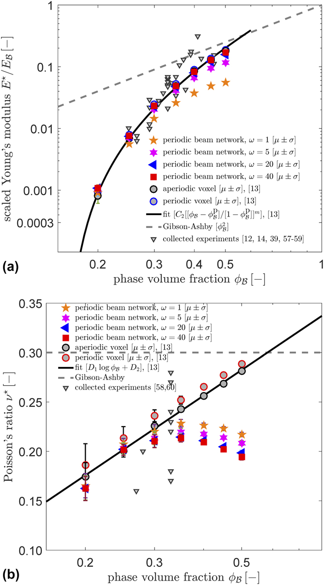
The variation of the computed effective Poisson’s ratio results are demonstrated in Fig. 9(b). Here, periodic and aperiodic voxel-based FE structures, a scaling law  ${\nu ^ \star } = {D_1}\log {\phi _{\cal B}} + {D_2}$ with D 1 = 0.116 ± 0.003 and D 2 = 0.363 ± 0.002 for the corresponding effective Poisson’s ratio as well as the experimental findings of Refs. Reference Briot, Kennerknecht, Eberl and Balk58 and Reference Lührs, Soyarslan, Markmann, Bargmann and Weissmüller60 are given. Like for the case of Young’s modulus predictions, the Gibson–Ashby model proposal of a constant Poisson’s ratio of 0.30 results in a considerable overestimation in the transverse strain to axial strain ratio for especially smaller volume fractions. Unlike the results for effective Young’s modulus, here we observe a good agreement with the voxel-based FE approach only for ${\phi _{\cal B}} \lt 0.35$. With increasing phase volume fraction for ${\phi _{\cal B}} > 0.35$, the effective Poisson’s ratio shows a decreasing trend unlike what is detected in the results of the voxel-based FE simulations. Recalling that the bulk Poisson’s ratio for gold is 0.44, this is attributed to the inability of the beam networks to reflect the bulk Poisson’s ratio for microstructures with higher phase volume fractions. Still, the results are in error margins of the experimental results of Refs. Reference Briot, Kennerknecht, Eberl and Balk58 and Reference Lührs, Soyarslan, Markmann, Bargmann and Weissmüller60.
V. CONCLUSIONS
In this study, a 3D microstructural beam-FE model generation method is proposed for the estimation of the effective elastic properties of nanoporous materials made by dealloying. The periodic beam-FE model is derived from homotopic medial axis skeletonization of the spinodal-like stochastic microstructures generated by Cahn’s method of computing leveled periodic random field composed of superposition of standing sinusoidal waves of fixed wave length. Circular cross-sectioned Timoshenko beams are used in the analysis to account for shear deformation effects. A 3D local thickness field computation is used for the detection of the diameter of the beams. To mimic the stiffening effects due to agglomeration of the mass in junctions, an increased Young’s modulus is assigned to the elements within the junction zone through a radially varying stiffness scaling factor. A detailed investigation of the influence of the stiffness scaling factor on the macroscopic response of beam-FE models for a wide range of phase volume fractions is presented. The results show that a stiffness factor of 40 gives a reasonable approximation for the Young’s modulus for the phase volume fractions  $0.20 \lt {\phi _{\cal B}} \lt 0.50$, whereas for the Poisson’s ratio, an agreement is due only for ${\phi _{\cal B}} \lt 0.35$.
As in the case of voxel-FE models of the identical random fields, the anisotropy indices of the elasticity of the generated beam-FE models show a sufficient proximity to isotropy.
Finally, it is demonstrated that as compared to the simulation statistics of voxel-FE models, it is seen that for the beam-FE models, one obtains over 500-fold computational acceleration with 250-fold less memory requirement.
ACKNOWLEDGMENT
We gratefully acknowledge financial support from the German Research Foundation (DFG) via SFB 986 “M3”, sub-project B6.


 Open access