
1. Introduction
Dialectologists have for quite some time been occupied with the question whether the areal distribution of syntactic phenomena is of a different nature than that of, for example, phonological or lexical ones and whether syntactic dialect areas exist at all (see, in general, Brandner, Reference Brandner2012:118; Glaser, Reference Glaser, Peter, Martin, Anja and Benedikt2013:201 for German and Szmrecsanyi, Reference Szmrecsanyi2013:1 for English). Doubt that syntactic phenomena can form areal patterns seems to be receding. It rather appears to have been more a consequence of insufficient data than a general immunity of syntax to geographical variation. Extensive research into dialect syntax from the 1990s onwards has shown clear evidence of the existence of syntactic areas (see Kortmann, Reference Kortmann, Peter and Jürgen Erich2010:846), although, as Glaser (Reference Glaser, Peter, Martin, Anja and Benedikt2013:204) puts it, “the distribution of morphosyntactic variants is quite inconspicuous in comparison with other linguistic levels.”
Whereas research into dialect syntax has mostly taken a qualitative approach, there are some quantitative analyses on the relationship between dialect variation in syntax and other linguistic levels (e.g., Spruit, Heeringa & Nerbonne, Reference Spruit, Wilbert and John2009 for Dutch and Scherrer & Stoeckle, Reference Scherrer and Philipp2016 for Swiss German), generally supporting the view of qualitative studies that syntax behaves differently. In these studies, however, data from different research projects conducted at different points in time are compared. Thus, it is possible that these results are impacted by differences in elicitation method, the choice of locations and speakers, and the time of elicitation. When comparing the Sprachatlas der deutschen Schweiz (SDS) with the Syntaktischer Atlas der deutschen Schweiz (SADS) for example (in the case of Scherrer & Stoeckle, Reference Scherrer and Philipp2016), one should keep in mind that the SDS was elicited using direct on-site fieldwork, whereas the SADS used questionnaires distributed by postal mail. Further, the SDS focused on NORMs (“non-mobile old rural males”; Chambers & Trudgill, Reference Chambers and Peter1998:29), whereas the SADS also includes other informant types, specifically women. While the SDS usually relied on one or two informants per location, the SADS aimed at receiving information from more than one person, with an average of 7.2 informants per location filling out all four questionnaires and 90% of the locations having between 5–10 informants, the other 10% showing only three or up to twenty-five informants (Bucheli Berger, Glaser & Seiler, Reference Bucheli, Claudia, Guido, Andrea, Adrian and Bernhard2012:101; Glaser & Bart, Reference Glaser, Gabriela, Roland, Alfred and Stefan2015:83–85). Finally, the SADS was conducted approximately half a century after the SDS, so language change occurring between the two datasets is another factor to be considered.
Against this backdrop, the present article will look at the very same dataset from two different angles, taking a computational approach comparing frequencies of annotated and unannotated data. In doing so, the study uses methods of “corpus-based dialectometry” in the vein of Szmrecsanyi (Reference Szmrecsanyi2013), albeit on atlas material. The material used is data from Syntax hessischer Dialekte (SyHD), a dialect syntax project carried out in the German state of Hesse. In this project, variables from a wide range of syntactic phenomena were investigated, mostly using the indirect method, that is, printed questionnaires to be filled out by the informants. This dataset is characterized in section 2. In section 3, we describe the methods that we use to measure linguistic distance before we present aggregate syntactic areas for the annotated syntactic data in section 4. In section 5, a subset of the data, translations from Standard German into the local dialect are analyzed using so-called character n-grams, or sequences of n characters, a common method in information retrieval and language identification. The idea is that the character n-grams include primarily phonological information that can be used for comparison to the syntactic data. The results of the syntactic and n-gram analyses are compared and further discussed in section 6, also with respect to their relation to Standard German. Section 7 summarizes the main conclusions and provides a brief outlook.
2. Background and data
The material used in this article is taken solely from the project Syntax hessischer Dialekte (SyHD), a dialect syntax project conducted in the German state of Hesse between 2010 and 2016 (see Fleischer, Kasper & Lenz, Reference Fleischer, Simon and Lenz2012; Fleischer, Lenz & Weiß, Reference Fleischer, Lenz, Weiß, Roland, Alfred and Stefan2015; Fleischer, Lenz & Weiß, Reference Fleischer, Lenz and Weiß2017). The project was carried out in the form of four questionnaire surveys and direct on-site fieldwork. The male and female informants were usually above sixty-five years old (average: 73.4 years old in the indirect survey, at the point of the first of the four written questionnaire surveys) and born in or close to the location surveyed. The selected locations usually counted about 500–1,500 inhabitants. The project sought to acquire informants who were prototypical NORMs, but also (in equal numbers) “NORFs,” that is, “nonmobile old rural females.” The selection of nonmobile older informants was due to a genuine interest in the syntax of traditional regional dialects in the state of Hesse. There existed hardly any information on syntactic structures in the dialects surveyed. Also, dialect speakers are rare or nonexistent in the younger generation in northern and central Hesse (Friebertshäuser & Dingeldein, Reference Friebertshäuser and Dingeldein1989: map 1; see also section 6.2), making the elicitation of comparable dialectal material for the entire area of investigation difficult in the younger generation.
Dialects in Hesse according to Wiesinger (Reference Wiesinger, Werner, Ulrich, Wolfgang and Herbert Ernst1983).
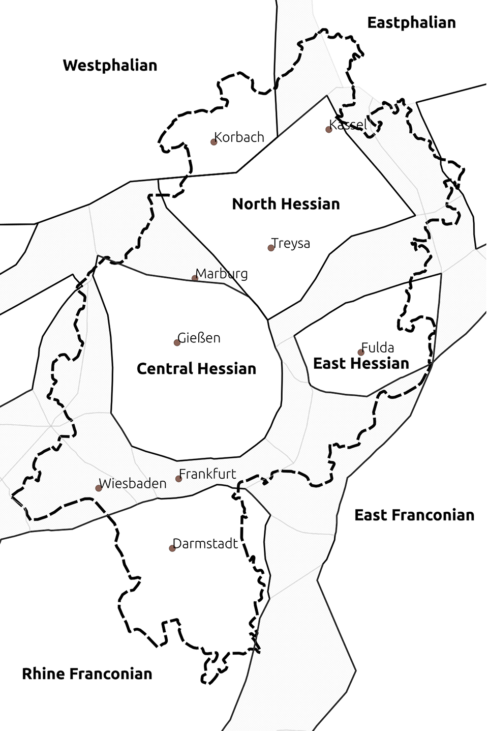
In the context of SyHD and thus in this paper, “Hessian dialects” refer to the German dialects spoken in the state of Hesse, which emerged in its current form only after the Second World War. The present-day state border is not of any traditional dialectological interest but was merely chosen for practical reasons. Interestingly, the state of Hesse has a heterogeneous dialect situation probably unparalleled within the German-speaking countries. Within Hesse, we find mostly various West Central German and thus High German dialects, but in the north, Low German—the other main branch of German dialects—is spoken. We also find transitional areas to East Central German and Upper German dialects in the east and south, respectively.
According to the most widely accepted classification of German dialects by Wiesinger (Reference Wiesinger, Werner, Ulrich, Wolfgang and Herbert Ernst1983, shown in Map 1 for Hesse, with a dashed line representing the state border), which is based on phonological and partly morphological criteria (Wiesinger, Reference Wiesinger, Werner, Ulrich, Wolfgang and Herbert Ernst1983:813), the West Central German dialects spoken in Hesse belong to four different groups, namely Rhine Franconian, Central Hessian, North Hessian, and East Hessian. Thus, even if the Low German dialects of Hesse, which are part of Westphalian and Eastphalian, respectively, are not counted as “Hessian,” it becomes clear that the terminological implications of “Hessian” have been, and to some extent still are, a moot point in German dialectology (see Birkenes & Fleischer, Reference Fleischer, Jürgen Erich and Joachim2019:435–440 on the terminological problems). Due to the decisive role of the High German consonant shift in traditional German dialectology and the fact that no consonant shift isogloss separates Rhine Franconian from the other West Central German dialects spoken in Hesse (i.e., Central Hessian, North Hessian, and East Hessian as of Wiesinger, Reference Wiesinger, Werner, Ulrich, Wolfgang and Herbert Ernst1983), the latter dialects were conceived of as a variant of Rhine Franconian (“North Rhine Franconian”) in many classifications. On the other hand, Bremer (Reference Bremer1892) and later Wiesinger (Reference Wiesinger, Reiner and Hans1980, Reference Wiesinger, Werner, Ulrich, Wolfgang and Herbert Ernst1983) made a case for an independent group of “Hessian” dialects separate from Rhine Franconian, with differing subgroupings (see Birkenes & Fleischer, Reference Fleischer, Jürgen Erich and Joachim2019:435–36). In comparison to Wiesinger’s (Reference Wiesinger, Werner, Ulrich, Wolfgang and Herbert Ernst1983) ternary distinction into Central Hessian, East Hessian, and North Hessian, in older classifications North Hessian and East Hessian often form a group of their own, leading to a binary distinction between “Upper Hessian” (roughly corresponding to Wiesinger’s Central Hessian) and “Lower Hessian” (roughly corresponding to Wiesinger’s North and East Hessian; see Birkenes & Fleischer, Reference Fleischer, Jürgen Erich and Joachim2019:439).
While Central Hessian is historically closer to Moselle Franconian, “Lower Hessian” is in many respects closer to the neighboring East Franconian and Thuringian dialects (see Birkenes & Fleischer, Reference Fleischer, Jürgen Erich and Joachim2019:441). In a general dialect geographical perspective, features from the Rhine Franconian varieties spoken in the south of Hesse, which comprise parts of the economically important area around Frankfurt, have been gaining ground in the south and center of the Central Hessian area for a long time (see most recently Vorberger, Reference Vorberger2019: chapter 3, and references cited therein).
The complete SyHD dataset consists of data from 149 locations within the state of Hesse. Additionally, twelve locations around Hesse (within a proximity of fifty to sixty kilometers) were chosen as points of comparison, leading to a total of 161 locations (Fleischer et al., Reference Fleischer, Lenz and Weiß2017:2).Footnote 1 The twelve locations outside of Hesse are omitted in this paper because they are geographical outliers. Due to incomplete questionnaires (see below), four of the 149 locations inside Hesse had to be excluded, leaving data from 145 locations for the present study. In Map 2, the 145 SyHD locations used in this article are plotted on top of Wiesinger’s (Reference Wiesinger, Werner, Ulrich, Wolfgang and Herbert Ernst1983) classification and the borders of Hesse (dashed line). The symbols are scaled after the mean number of responses per location.
The 145 SyHD locations used in this article.

The present paper only uses the SyHD data elicited by means of the indirect method (i.e. the four written questionnaires). By doing so, more data points for more phenomena are available (a median of four informants per location compared to one informant in the direct survey). The consequences should be negligible: as Fleischer et al. (Reference Fleischer, Lenz, Weiß, Roland, Alfred and Stefan2015:279) and Lenz (Reference Lenz, Augustin and Philipp2016:213) show, the differences in the results for the same phenomena between the indirect and direct methods are small. The dataset of the indirect survey comprises 122 variables or syntactic phenomenaFootnote 2 elicited using various methods such as assessment, fill-in and puzzle tasks, translations, and descriptions of pictures and picture sequences (see Fleischer et al., Reference Fleischer, Simon and Lenz2012). All in all, the assessment tasks dominate with approximately 75% of all questions being of this type (Fleischer et al., Reference Fleischer, Lenz, Weiß, Roland, Alfred and Stefan2015:265). In the assessment tasks, informants were given a description of a situation or context and then had to select possible answers by checking boxes. Additionally, they could indicate their own alternative by writing down their own version. Finally, they had to identify the construction that they judged best as the “most natural” one (see Fleischer et al., Reference Fleischer, Simon and Lenz2012:13–17). As Glaser (Reference Glaser2000:267) remarks, individual variation seems to be more common in syntax than elsewhere and, therefore, many variants may coexist in the active and passive competence of a dialect speaker. Choosing the “most natural” variant is therefore a means of reducing the idiolectal variation. In the present paper, we will restrict the dataset to the “most natural” variants in the assessment tasks.
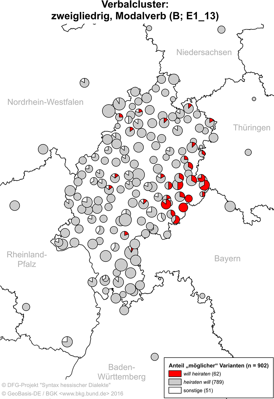
The primary results of SyHD have been published in SyHD-atlas, being both a web applicationFootnote 3 and a quotable PDF version (Fleischer et al., Reference Fleischer, Lenz and Weiß2017). It consists of twenty-nine articles on the phenomena surveyed. To every question contained in the questionnaires at least one map is offered in SyHD-atlas. In some instances, more than one variable per question was annotated (see note 2). Map 3, taken from Weiß and Schwalm (Reference Helmut and Schwalm2017:475), a description of the serialization of verbal clusters in SyHD-atlas, illustrates the mapping technique used in the project. At every location, a pie chart represents the number of answers displaying a certain construction (in the case at hand, ascending and descending serialization of modal and lexical verbs, as illustrated by ob er einmal heiraten 2 will 1/will 1 heiraten 2 ‘if he ever will intend to marry’). The size of the symbol is scaled to the amount of (sensible) answers per location. As informants had the possibility to indicate more than one variant, the number of answers can be higher than the number of answered questionnaires at the respective location. On the other hand, occasionally informants left a question unanswered or they provided nontarget-like responses, inevitably resulting in fewer responses than answered questionnaires.
SyHD map showing verbal clusters (Weiß & Schwalm, Reference Helmut and Schwalm2017:475).
3. Methods: Measuring and visualizing linguistic distance
This section gives a brief introduction into the data aggregation, comparison and dimension reduction techniques used in this paper.Footnote 4 Our central goal is to compare the distributions of variables between the locations. Many measures of similarity or distance could be used. In dialectometry, one of the established measures for categorial data (like syntactic variants of a variable) is Goebl’s “Relativer Identitätswert” (RIW) (see, for example, Goebl, Reference Goebl1984, Reference Goebl, Alfred, Roland and Stefan2010), defined simply as the quotient of the number of identical features and the number of all features between two locations (outside of dialectometry, this measure is mostly known as “relative Hamming similarity”). One general problem with the RIW—at least in its original implementation on a “location by taxate” matrix—is that it does not cope with multiple variants in one location. Goebl’s Salzburg school of dialectometry reduces the original data to one variant per location if there is intralocal variation. However, intralocal variation (as well as variation determined by other factors) is a key fact of human language. Therefore, we follow Nerbonne and Kleiweg (Reference Nerbonne and Peter2003) in not reducing multiple answers per location.
The creators of the SyHD project, like those of other recent dialect syntax projects, explicitly aimed for a solid empirical basis with multiple informants per location. In the raw dataset, the number of location x variable pairs with multiple variants per location is found in 62.5% of all cases. Using RIW would thus imply an extreme reduction of the data. One possible way of reducing the variation per location would be to aggregate the data and select the majority variant, but on many occasions, no such majority can be found and then one would have to choose a random variant or resort to a set comparison, like Scherrer and Stoeckle (Reference Scherrer and Philipp2016:100) did for the SDS and SADS data. Compared to the latter study, however, where multiple dominant variables made up 3.5% of the cells, this is as high as 11.4% in the SyHD data.Footnote 5
The present paper takes another approach and uses a measure of similarity that takes local frequency distributions into account, namely cosine similarity, which is often used in text mining to discover linguistic or topical similarities between documents comparing the frequencies of the terms in these documents (see Manning and Schütze, Reference Manning and Schütze1999). In the context of this study, cosine similarity is used to compare the frequency distributions of the individual syntactic variants between locations.Footnote 6 The idea behind cosine similarity is to compare two lists or vectors, that is, the frequencies of all syntactic variants in two locations, by computing the cosine of the angle between them, where each feature variant represents one dimension in the vector. A cosine similarity of zero indicates that the locations (in terms of the compared feature frequencies) are completely different (90° angle), a cosine similarity of one (0° angle) means that they are identical in terms of the variables explored.Footnote 7 In this way, we have a computational means of measuring similarities between locations as similarities in the distribution of variants of linguistic variables. In what follows, we will work with the distances, since this is required for many of the methods used in this paper. This is done simply by subtracting the cosine similarity from one.
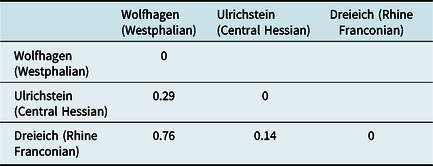
As stated in section 4, 117 maps from the indirect survey form the data basis of this analysis. For each syntactic variable (or map), all variants were extracted together with their absolute frequencies in a “location x variant” matrix. Due to differences in the number of respondents in the four different surveys and differences in the number of responses per variable,Footnote 8 the variant frequencies had to be converted into weights between zero and one (frequency of one variant/frequency of all variants of a variable in one location). For example, looking at the variants of one variable, simple past versus periphrastic perfect in a weak verb (wohnen ‘live’), a simplified location x variant matrix could look like shown in Table 1. As an example, only three locations with absolute and relative frequencies of the variants are given (note that only the relative frequencies are used for comparison). We notice a pattern here: Westphalian Wolfhagen shows exclusively simple past forms, whereas Central Hessian Ulrichstein and Rhine Franconian Dreieich show variation between periphrastic perfect and simple past. In Central Hessian Ulrichstein, 50% of the answers consist of simple past, whereas in Rhine Franconian Dreieich the quotient is only 1/5. Thus, it seems like Westphalian Wolfhagen and Rhine Franconian Dreieich are further apart from each other than Westphalian Wolfhagen from Central Hessian Ulrichstein and Central Hessian Ulrichstein from Rhine Franconian Dreieich.
Frequency distributions of two variants of the past tense in three locations

We can compare these distributions numerically using a similarity measure. Note that the RIW measure discussed above would be forced to select one of the two variants in Central Hessian Ulrichstein (both being of the same frequency), whereas using cosine similarity this variation can be neatly accounted for. Cosine similarityFootnote 9 is calculated as follows (Manning & Schütze, Reference Manning and Schütze1999:300):
 $$cos\left( {\vec x, \vec y} \right) = {{\vec x\cdot\vec y} \over {\left| {\vec x} \right|\left| {\vec y} \right|}} = {{\sum\nolimits_{i = 1}^n {{x_i}} {y_i}} \over {\sqrt {\sum\nolimits_{i = 1}^n {x_i^2} } \sqrt {\sum\nolimits_{i = 1}^n {y_i^2} } }}$$
In cosine similarity, the angle between two vectors ( $\vec x, \vec y$
) is measured. These vectors are the rows in Table 1 containing variant frequencies for each location. In the following example, we will compare Westphalian Wolfhagen and Rhine Franconian Dreieich, where we expect the greatest distance. This first involves calculating the so-called dot product between the two vectors (2) and then the Euclidean norm for each of them individually like in (3) and (4):
$\vec x, \vec y$
) is measured. These vectors are the rows in Table 1 containing variant frequencies for each location. In the following example, we will compare Westphalian Wolfhagen and Rhine Franconian Dreieich, where we expect the greatest distance. This first involves calculating the so-called dot product between the two vectors (2) and then the Euclidean norm for each of them individually like in (3) and (4):
 $$\vec x*\vec y = \left( {1*0.2} \right) + \left( {0*0.8} \right) = 0.2$$
 $$\left| {\vec x} \right| = \sqrt {\left( {\left( {1*1} \right) + \left( {0*0} \right)} \right)} = 1$$
 $$\left| {\vec y} \right| = \sqrt {\left( {\left( {0.2*0.2} \right) + \left( {0.8*0.8} \right)} \right)} = 0.82$$
On this base, we can calculate the cosine between the two locations by dividing the dot product of ( $\vec x, \vec y$
) by the product of the squared dot products of each individual vector
$\vec x, \vec y$
) by the product of the squared dot products of each individual vector $\vec x$
and
$\vec x$
and $\vec y$
:
$\vec y$
:
 $$0.2/\left( {1*0.82} \right) = 0.24$$
The cosine distance is now simply:
 $$1 - 0.24 = 0.76$$
We now compute the pairwise distances in a similar manner for all other combinations, which produces the distance matrix shown in Table 2 for the three locations. We notice that of the three sensible combinations—the distance between one location and itself is of course zero, and the direction of the comparison is not relevant—the distance between Westphalian Wolfhagen and Rhine Franconian Dreieich is the furthest (0.76). We also notice that Central Hessian Ulrichstein takes an intermediate position, but it is closer to Rhine Franconian Dreieich (0.14) than to Westphalian Wolfhagen (0.29).
Cosine distance for three locations
When the methods described above are applied to the whole dataset, the resulting distance matrices are quite large (145 locations x 145 locations). In order to visualize the similarities between locations on a traditional map, we need to reduce these data. In this paper, we settled on multidimensional scaling and cluster analysis as methods of data reduction for visual display.
Multidimensional scaling (MDS) aims at visualizing the distances between data points in low-dimensional space (i.e., mostly in two or three dimensions; Levshina, Reference Levshina2015:336). In the Groningen school of dialectometry (see, for example, Heeringa, Reference Heeringa2004), the three first dimensions of an MDS solution are projected to a two-dimensional map where each dimension is represented as different intensities of red, green, and blue (i.e., an RGB scale is used). Ideally, the first three dimensions can account for most of the variation in the data matrix, and the method makes it possible to project this information onto a map. Accordingly, this map can also readily be compared with older classifications. There exist many different MDS techniques (e.g., Classical [Metric] MDS, Kruskal’s nonmetric MDS, and Sammon’s Non-Linear Mapping). Similar to Heeringa (Reference Heeringa2004:160–61), we tested the three mentioned techniques and computed the r2 value for each, that is, the amount of variation in the original distance matrix explained by the MDS solution. This is simply the squared Pearson’s correlation between the original distance matrix and the Euclidean distance between the points of the MDS solution. A value above 0.6 is favorable (Spruit, Heeringa & Nerbonne, Reference Spruit, Wilbert and John2009:1632).
In the resulting MDS maps, identifying or making comparisons to traditional dialect groups can be somewhat tricky due to their continuum-like nature. We therefore also apply cluster analysis to our data. We experimented with a wide range of clustering algorithms (both hierarchical and partitioning methods). While UPGMA (Sokal & Sneath, Reference Sokal and Sneath1963) had the best cophenetic correlation coefficient of all methods (similar to Heeringa, Reference Heeringa2004:151 and Lameli, Reference Lameli2013:182–83) and thus gave the best representation of the distance matrix, it suffered from a chaining effect (probably due to idiosyncratic responses) and was thus not successful in finding groups (see Lameli, Glaser & Stöckle, Reference Lameli, Elvira and Stöckle2020:42 for a similar finding on Swiss German data). Ward’s algorithm (Ward, Reference Ward1963), yielding somewhat lower correlations, did not show this effect. We settled on Ward because it is a quasistandard in dialectometry and has been used in comparable studies such as Scherer & Stoeckle (Reference Scherrer and Philipp2016) for Swiss German data. Of the partitioning methods, we use k-medoids (Kaufman & Rousseeuw, Reference Kaufman, Rousseeuw and Yadolah1987), which is less sensitive to outliers than its sister k-means.
In cluster analysis, choosing the optimal number of clusters is nontrivial (Moisl, Reference Moisl2015:215). Here, we determined the optimal number using the average silhouette width, which is a common measure for the presence of structure in a clustering solution. As a rule of thumb, the average value should be higher than 0.2 (Levshina, Reference Levshina2015:311). Furthermore, unlike MDS, cluster analysis is rather unstable in that small changes to the data may result in very different clusters. In order to assess the stability of the clusters found, we used bootstrapping (see, for example, Nerbonne et al., Reference Nerbonne, Peter, Wilbert, Franz, Christine, Hans, Lars and Reinhold2008 and Lameli, Reference Lameli2013:188–91). The distance matrices were re-sampled one thousand times, and the various clusterings were then compared to the original clustering via set comparison (Jaccard similarity), a value between zero and one (Hennig, Reference Hennig2007). The closer to one, the more stable the cluster. Following the R package fpc (Hennig, Reference Hennig2018), we regard a value above 0.75 as stable. When deciding upon the optimal cluster solution, we looked at the cluster solutions with the highest silhouette width and the highest cluster stability.
4. Results: Syntactic areas in the dialects of Hesse
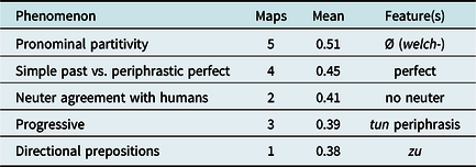
The data from the SyHD indirect survey cover various phenomena that were assigned to one of the following six areas (for mainly practical reasons): verbal syntax, (pro-)nominal syntax, agreement, word order, clause connection, and other (various) phenomena. They were chosen according to research interests in dialect syntax and not merely for the sake of geography (Fleischer et al., Reference Fleischer, Lenz, Weiß, Roland, Alfred and Stefan2015:267). For this study, all phenomena except the numerals were included with all variants.Footnote 10 In Table 3, the phenomena and the number of maps for each phenomenon are listed. We notice that some phenomena, like partitive pronouns and progressive constructions, at first sight appear to be overrepresented. We did not attempt to reduce this bias in any way. All in all, this is a problem of linguistic atlases and “atlas-based dialectometry” in general (Szmrecsanyi, Reference Szmrecsanyi2013), since usually only phenomena that display areal variation are mapped at all in linguistic atlases.Footnote 11 Equally, it is often considered justified that more complex syntactic phenomena should receive more attention. For instance, it has long been known that the verb type plays a role in the distribution of the simple past and the periphrastic perfect in German dialects. Thus, various verbs were used in exploring this phenomenon (see Fischer, Reference Fischer2017:27–28). Similarly, for periphrastic constructions thought to encode progressive meaning, verb class as well as the presence or absence of an object are important factors, which was reflected in the SyHD questionnaires. The same holds for pronominal partitivity, for which, among other factors, the number and gender of the noun are important, making it necessary to elicit the same “construction” in various linguistic contexts.
SyHD phenomena included in this study
The syntax dataset is based on 117 variables and contains 70,898 responses in total. The SyHD dataset (without the reductions in this article and counting only the “most natural” variants) comprises 122 variables and 85,141 responses. Thus, we consider 82% of the material here. Some locations have more informants than others. There is, however, no correlation between linguistic distance and the number of informants per location (r = 0.003, p = 0.443, Mantel test with 1,000 permutations). The data are fairly normally distributed with a slight negative skew, which means that there are a few more data points showing smaller distances than larger, but all in all the skewness and kurtosis values (−0.04 and −0.4, respectively) are within an acceptable range of a fairly normal distribution (Szmrecsanyi, Reference Szmrecsanyi2013:72). The minimal distance is between two close Rhine Franconian locations (Biblis/Nordheim and Bensheim/Schwanheim), the furthest distance is between East Hessian Ehrenberg/Wüstensachsen and Westphalian Twistetal/Twiste. As we shall see in the following, East Hessian is syntactically probably the most exotic Hessian dialect group, whereas the Low German (and North Hessian) locations show a lot of correspondence with Standard German syntactically.
4.1 Multidimensional scaling
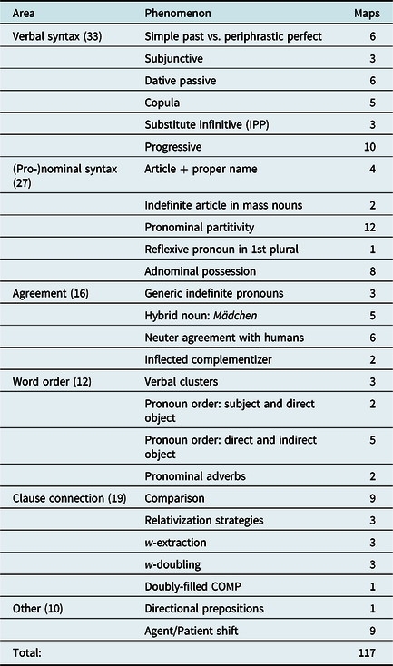
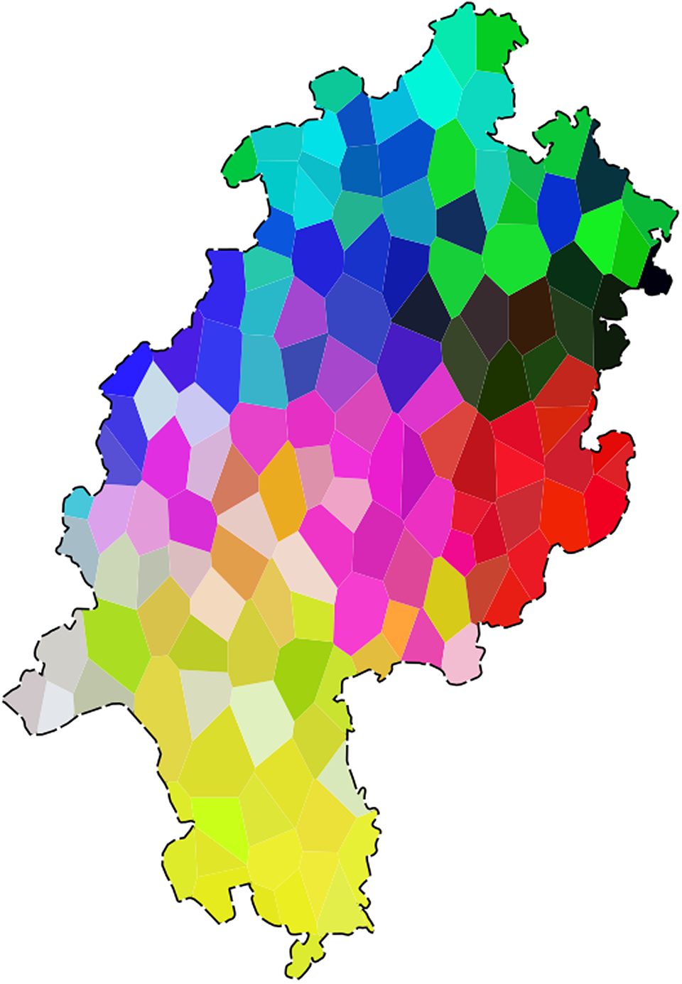
We first apply multidimensional scaling to the distance matrix. Kruskal’s method yielded the highest r2 value (= 0.895) for three dimensions. We follow Heeringa (Reference Heeringa2004) in mapping the individual dimensions of an MDS solution to an RGB scale, so that similar colors indicate similar dialects. The result is seen in Map 4. Different from other studies mapping MDS solutions, however, we refrained from polygonizing the area of investigation, using point symbol maps instead here (but see section 6.1 and Map 21 for a visualization of the same data with a polygonized area of investigation).
MDS/Heeringa of annotated syntax data, Kruskal MDS (r2 = 0.895).
First and foremost, we see no apparent difference between Low German and neighboring High German. Whereas East Hessian and Rhine Franconian appear as rather homogeneous, the structures in Central Hessian, North Hessian, and Low German are of a different character. Central Hessian appears to be the most heterogeneous area, with influences from all other areas. Parts of southern Central Hessian seem to be closer to Rhine Franconian, which could be due to expansion of Rhine Franconian forms, for which this area is known (see Vorberger, Reference Vorberger2019: chapter 3; Birkenes & Fleischer, Reference Fleischer, Jürgen Erich and Joachim2019:441). The northwestern parts, on the other hand, seem to be closer to North Hessian. The core of Central Hessian is closest to East Hessian.
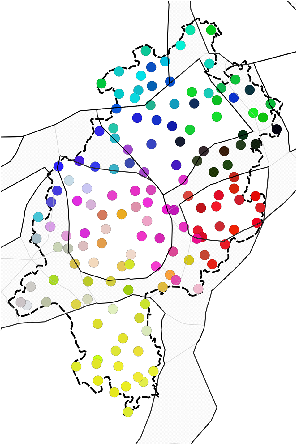
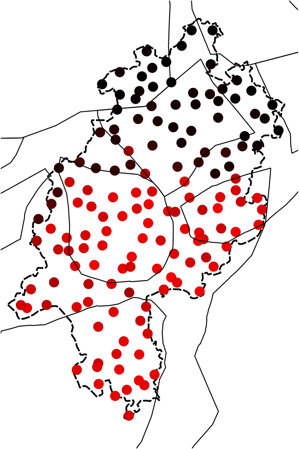
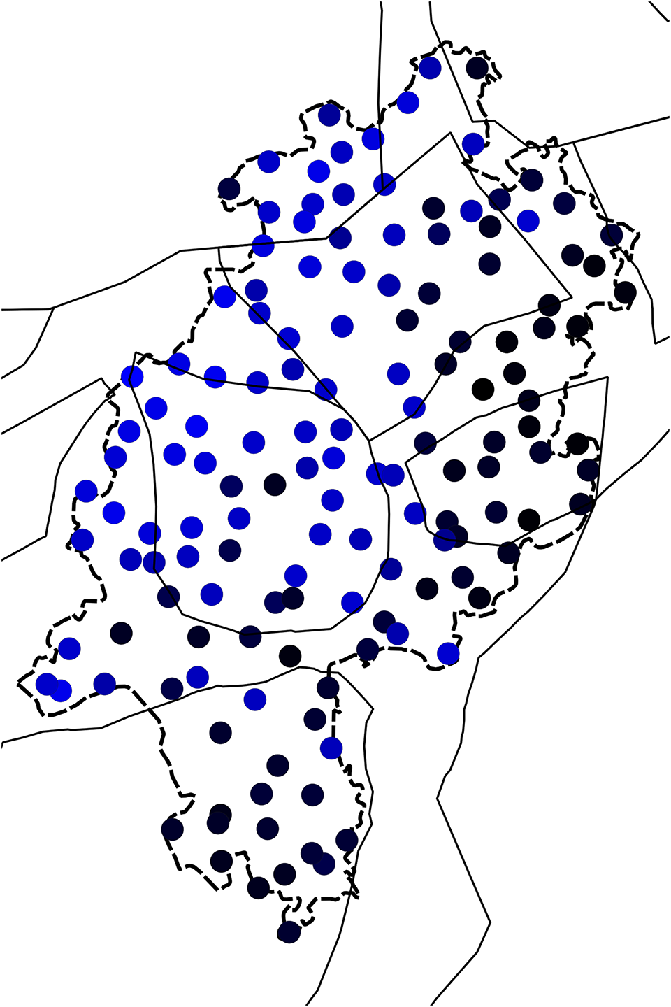
It is also instructive to investigate the individual dimensions of the MDS solution, as shown in Maps 5, 6, and 7 (note that as in Map 4, black color means no participation in the respective dimensions). We notice that the most important border (i.e., the first dimension), explaining 67.9% of the variation, is between Low German plus North Hessian plus parts of northwestern Central Hessian versus the rest. In the second dimension, which accounts for 14.7% of the variation, it is primarily East Hessian and southern North Hessian plus some scattered further locations that are opposed to the rest. The third dimension, accounting only for 6.9% of the variation, is more disparate. In all dimensions, Low German and North Hessian behave similarly to a large extent, which we would not expect based on traditionally assumed dialect areas.
Dimension 1 of annotated syntax data (67.9%).
Dimension 2 of annotated syntax data (14.7%).

Dimension 3 of annotated syntax data (6.9%).
4.2 Cluster analysis
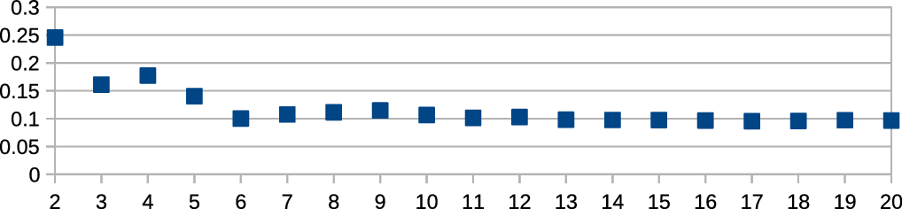
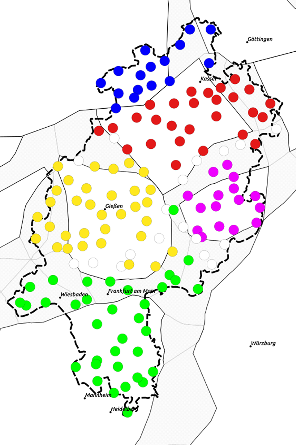
Using the average silhouette width as a criterion for the optimal number of clusters, a two-cluster solution is clearly preferable in both Ward and k-medoids on the syntax data. This is shown by Figures 1 and 2, which show the average silhouette widths for cluster solutions from two to twenty for both Ward and k-medoids. As Figures 1 and 2 indicate, two-cluster solutions are best with both algorithms. The areal distribution of the two clusters is illustrated in Maps 8 and 9. Note that white color in the k-medoids solution (Map 9) indicates locations with a very low silhouette width (< 0.05): The assignment of these locations to one of the clusters is unclear.
Ward: two clusters (annotated syntax data).
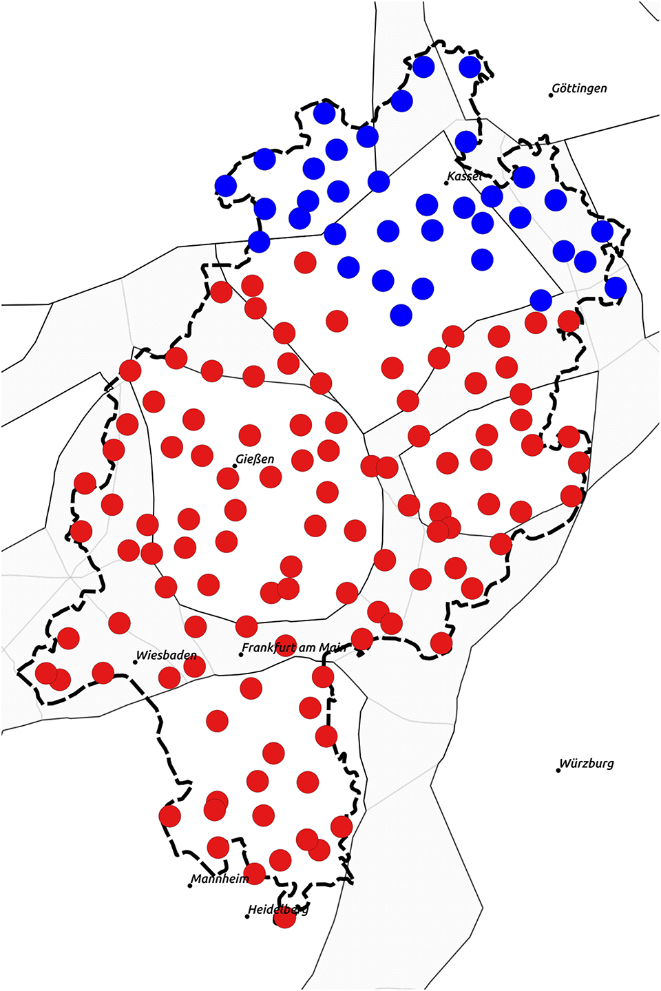
k-medoids: two clusters (annotated syntax data).

Average silhouette width (Ward), syntax data.

Average silhouette width (k-medoids), syntax data.
The two models differ in that in k-medoids the border is somewhat further to the south than in Ward, partially due to the uncertain locations in the former model. Both cluster solutions are stable when using bootstrapping. The k-medoids solution is more similar to the first dimension of the MDS above, with one cluster covering Low German plus North Hessian (plus some northwestern Central Hessian locations).
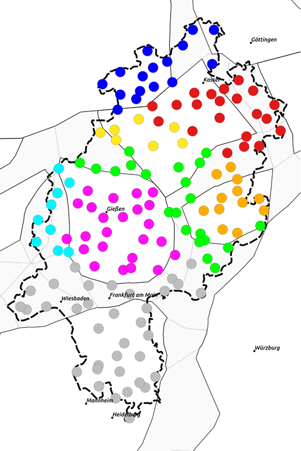
We also discuss the second-best solution, which is three clusters in Ward and four clusters in k-medoids, shown in Maps 10 and 11, respectively. In the k-medoids solution, all four clusters appear stable, whereas in the Ward solution, one of three clusters is unstable (East Hessian). The k-medoids solution reveals a certain variability of Central Hessian, which is also shown by the MDS model. Therefore, we will proceed with the k-medoids model, omitting the uncertain locations, and look at the features that are most characteristic for its four groups in the next section.
Ward: three clusters (annotated syntax data).

k-medoids: four clusters (annotated syntax data).

4.3 Prominent features
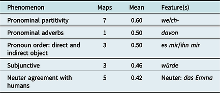
In order to identify prominent features for the four clusters, we resort to a simple effect size measure: the mean difference. We calculated the mean weight for each feature for each of the four clusters and compared this mean value with the mean value for all other clusters. The closer the resulting value is to one, the more prominent is the feature for the cluster. We only look at features with a mean difference of more than 0.25 (see Table 3 for a list of all phenomena).
In the northern cluster represented by blue symbols in Map 11, encompassing Low German and parts of North Hessian, we find syntactic features that are typical for Standard German in many (though not all) instances, shown in Table 4. This includes the use of welch- in indefinite partitive contexts (cf., Standard German da sind welche, literally ‘there are <such> ones’), no splitting of pronominal adverbs (Standard German davon weiß ich noch nichts instead of da weiß ich noch nichts von literally ‘I know nothing thereof’), pronominal direct objects preceding pronominal indirect objects and the use of würde (as opposed to täte) in the subjunctive. One notable exception is the use of neuter agreement forms for female persons (e.g., s Maria, literally das Maria; see Leser-Cronau, Reference Leser-Cronau2017; Birkenes & Fleischer, Reference Fleischer, Jürgen Erich and Joachim2019:464), which is not found in Standard German.
Defining features of the “Low German/North Hessian” cluster
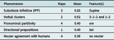
In the western central cluster represented by red symbols in Map 11, encompassing most of Central Hessian and some adjoining areas, the mean values are remarkably lower (Table 5), which indicates that there are fewer features associated solely with this region. The most important features are the partitive particles sen and ere corresponding to Standard German welch- (e.g., Do soi ere ‘there are part.’ This is a well-known feature, which also occurs in East Hessian (Birkenes & Fleischer, Reference Fleischer, Jürgen Erich and Joachim2019:464). Other characteristic features include the tun periphrasis in progressive contexts—sie tut beten ‘she is praying’ (literally ‘she does pray’)—and the reflexive pronoun sich, restricted to the third person in most German varieties, in first-person plural contexts, like in mir duze sich häi ‘we are on a first-name basis here’ (literally ‘we say you:2sg to each other here,’ ‘we thou each other here’; Birkenes & Fleischer, Reference Fleischer, Jürgen Erich and Joachim2019:464).
Defining features of the “Central Hessian” cluster

In the mideastern cluster represented by green in Map 11, encompassing most of East Hessian, supine forms and verb clusters with the finite verb in the second last position are characteristic (Table 6; the areal distribution for one phenomenon, two-verb clusters, is illustrated in Map 3). This East Hessian cluster is similar to Central Hessian in that the indefinite partitive particle ere is used here as well. Of all clusters, the mean difference values for East Hessian are the highest, meaning that here we find the most distinctive features. This fits well with the MDS and cluster models above, where East Hessian always forms an area of its own.
Defining features of the “East Hessian” cluster
In the southern cluster represented by yellow in Map 11, which corresponds to Rhine Franconian, the characteristic structures illustrated in Table 7 are also known for Upper German. We notice Ø in partitive constructions (which is also typical for Alemannic; see Fleischer, Reference Fleischer, Jürgen Erich and Joachim2019:644 and references cited therein) and periphrastic perfect instead of simple past (see Fischer, Reference Fischer2017, Reference Fischer2018). For this phenomenon, which can be found in the SyHD data in accordance with older descriptions, the so-called “Mainlinie” (see Durrell, Reference Durrell, Wolfgang, Werner and Peter1989, esp. 94–95) splits Hesse into two parts with simple past in the center and the north and periphrastic perfect in the south.
Defining features of the “Rhine Franconian” cluster
4.4 Intermediate summary
All in all, it turns out that, irrespective of the method, the emerging syntactic areas only partially correlate with known dialect areas. Most importantly, the Low German-High German border is not reflected in the data at all. On the other hand, East Hessian occupies a special position in displaying many features deviating from other areas. In the next section, we will pursue the question as to whether traditional dialect areas are reflected in the SyHD data if nonsyntactic phenomena are taken into account.
5. A comparison with n-grams
To compare the syntactic data of chapter 4 with another data type, we additionally performed n-gram analyses with a selection of the very same dataset. n-grams are sequences of n linguistic items, that is, characters or words. Whereas word n-grams are often used in syntactic and semantic research, character n-grams are popular in language identification tasks (see, for example, Cavnar and Trenkle, Reference Cavnar and Trenkle1994). All in all, n-grams are very common in computational linguistics, but not very much used in dialectometry for the time being (but see Birkenes, Reference Birkenes2019, Reference Birkenes2020).
Creating character n-grams is simple. One starts with the first character in the text and from there extracts the next n characters, moves to the next character and repeats this procedure until the end of the text has been reached. Finally, the sequences are counted, yielding a frequency list. In comparison to frequently used Levenshtein distances, with character n-grams there is no need for (often time-consuming) alignment. On a more theoretical level, character n-grams have the important advantage that missing values, which almost certainly occur in every dialect atlas data base, do not have to be imputed (see Lameli et al., Reference Lameli, Elvira and Stöckle2020:36 on this problem).
For the n-gram analyses, we selected all “free answers” from six tasks in which informants were instructed to provide translations of Standard German sentences into the local dialect.Footnote 12 These tasks were originally intended to investigate the distribution of the simple past versus the periphrastic perfect (three tasks), agreement (one task), word order (one task), and relativization strategies (one task). The stimulus sentences are shown in Table 8, each together with one example translation from Central Hessian Ulrichstein. The total corpus has a size of 37,121 word tokens (without punctuation), that is, 256 tokens per location.Footnote 13 As holds generally for the SyHD material, each location had multiple respondents, with an average of 5.8 responses per location. Note that this is slightly more than the average of five replies to all syntactic questions from section 4. This means that the translation tasks produced more responses than the assessment tasks, which make up the majority of the SyHD material (see section 2). The various free-text responses were simply aggregated for each location. In this way, variation within one location is taken care of to a certain extent, as this will be reflected by the resulting frequency profiles.Footnote 14
Translations task stimuli and dialectal translations from one informant
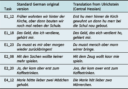
It is important to note that the dialect translations produced by the SyHD informants are not phonetically (or phonologically) exact transcriptions. Rather, we are dealing with “layman transcriptions” for which the informants adapted Standard German orthography to express dialect characteristics in a way they judged best, with no instruction as to how to deal with phenomena that might be difficult to express. It is expected that certain dialect traits will have no adequate rendering in such material. However, as will be discussed below, clear areal patterns can be deduced from these nonoptimal data, which replicate known dialect structures to a large extent. Despite the inevitable inaccuracies, layman transcriptions provide fairly exact information on the areal distribution of many phenomena. To note one prominent example, for almost a century scholars have been debating the accuracy of the layman transcriptions of Georg Wenker’s Sprachatlas des Deutschen Reichs. Suffice it to note here that the areal distribution of many, though not all, dialect phenomena is rendered “clearly and exactly” [our translation], as Schirmunski (Reference Schirmunski1962:82) puts it. In contrast, it has often been observed that “fieldworker isoglosses” represent a major pitfall in directly elicited atlas material (see, for example, Nerbonne & Kleiweg, Reference Nerbonne and Peter2003:341–43; Mathussek, Reference Mathussek2014:215–18 and 238–41; Mathussek, Reference Mathussek, Marie-Hélène, Remco and John2016). Clearly, we are able to avoid this problem in our indirectly elicited dataset.
Character n-grams provide a global measure of string similarity. Obviously, phonological information dominates in lower-order n-grams (for instance, n-grams representing certain sounds or combinations of sounds only or dominantly prevalent in a certain dialect group). However, morphological information (e.g., in characteristic morphemes, leading to higher frequencies of certain n-grams) is also present to a certain extent, and the same goes for lexis, if, for instance, n-grams contained in a word type not cognate to other word types and only present in a certain area turn out to be characteristic. Even syntactic information can contribute to the frequency of certain character n-grams. For instance, in a dialect that uses the definite article also with proper names, the frequency of n-grams with definite articles will be higher, and dialects with loss of the simple past will have a higher proportion of n-grams occurring in periphrastic-tense auxiliaries (Standard German sein ‘to be’ and haben ‘to have’) or in ge- prefixes (e.g., represented as geX- or gXY- depending on whether syncope has taken place), occurring in the past participles used in the periphrastic perfect forms.
In order to ensure comparability, some degree of text normalization is in order. In this process, maximizing comparability while minimizing information loss is key. We decided to apply the following simple normalization steps:
-
1. convert all letters to lowercase letters
-
2. strip all punctuation
-
3. reduce all diacritics except umlaut to the base character
Capitalization of letters is subject to variation in German writing and not relevant here since we are not interested in parts of speech. The same goes for punctuation since it does not provide relevant cues for the following investigation. We are only considering character sequences delimited by word boundaries. The last step is potentially controversial, but we would like to note that the informants rarely used any diacritics besides the umlaut anyway. There are fewer than twenty instances of circumflex and acute accent in the whole corpus, which merely make up a fragment of the data. Thus, removing these for the sake of comparability seems like a valid decision.
For each location, then, n-grams are formed on the basis of the translations. Examples of n-grams created using the sentence Du musst mersch aber morn wirrer bringe (E1_23 from an informant of the Central Hessian location of Ulrichstein), translating the Standard German template Du musst es mir aber morgen wieder zurückbringen! ‘You have to bring me it back tomorrow, however!’ are shown in Table 9 (spaces are indicated by ‘_’). In the present paper, we will only be concerned with character trigrams. Obviously, unigrams are not very informative (although they may be suitable for simple language identification), but bi- and trigrams contain more relevant information such as diphthongs and phonotactics. We settled on trigrams because they allow us to capture certain endings and consonant clusters in addition to word boundaries. We do not consider trigrams spanning word boundaries (e.g., <u_m>, <h_a> and so on in the example in Table 9). Trigrams spanning word boundaries might be characteristic and even contain information on word order, as they might be indicative for certain serialization patterns. However, it seems sensible to reduce syntactic information here, given that the trigram data are compared to the annotated syntactic data. This was also done for practical reasons since word-spanning trigrams are more difficult to interpret.
Character n-grams of Du musst mersch aber morn wirrer bringe. from Ulrichstein (E1_23)

The next step involves counting the trigrams, thus creating trigram profiles. In Table 10, three such profiles (illustrating the top ten trigrams in the corpus only) are shown for the three locations discussed in section 3. We note that <er_>, the most frequent trigram in the corpus, is more common in Wolfhagen than in the two other locations. Equally, other trigrams show characteristic local preferences. After counting the trigrams, frequency cuts were applied to the frequency lists. For each trigram to be part of the inventory, it had to be found in at least two locations and have a minimum frequency of five across the corpus (see below). Doing so reduces the sparsity considerably, which is an advantage when dealing with high-dimensional material. In order to lessen the effect of the Zipfian distribution, logarithmic weighting (base 2) was applied to the frequency lists. This reduces the effect of asymmetries in trigrams found in most documents. When using the raw frequencies, we found that differences regarding certain endings, such as -e and -n, became dominant. When applying cosine distance (as described in section 3) to the log-weighted frequency matrix, we get the distance matrix in Table 11 for the three locations.
The corpus’ top ten trigrams in three locations

Cosine distance (n-grams)

We see that Central Hessian Ulrichstein and Rhine Franconian Dreieich are both quite distant from Westphalian Wolfhagen (0.41 and 0.43, respectively), as might be expected due to the difference between Low and High German, and much closer to each other (0.21). This is different from the syntax data discussed in section 3, where Central Hessian Ulrichstein, in terms of past tense behavior, was not quite as far from Wesphalian Wolfhagen as Rhine Franconian Dreieich was. In terms of geographical distance, we would suppose that Rhine Franconian Dreieich would be further away from Westphalian Wolfhagen than Central Hessian Ulrichstein. In this example, this does not appear to be the case, however.
Using the procedure just described, n-grams were extracted for all 145 locations. Without any frequency cuts, the 37,121 words of the corpus yield 99,095 trigram tokens and 2,205 trigram types. Many trigrams only occur in single locations, however, leading to a high sparsity (86.7%), that is, a matrix with many zero values. As already indicated, we thus excluded trigrams only found in a single location, as well as trigrams with an absolute frequency lower than five (which we set as an arbitrary threshold). In the end, we had 97,271 trigram tokens and 1,121 trigram types with a sparsity of 74.9%. The distance matrix consists of 10,440 comparisons between 145 locations. The data are fairly normally distributed. The skewness is .17, meaning that there are more data points showing larger distances than smaller ones.
The minimum distance is between two geographically close locations in the Rhine Franconian dialect area (Bad König/Ober-Kinzig and Mossautal/Hüttenthal). The maximum distance is between Liebenau/Ostheim, a dialect in the Low German transitional zone between Westphalian and Eastphalian, and Dillenburg/Eibach in the Central Hessian area. This is somewhat unexpected from a geographical point of view, as these two locations are only 110 km apart from each other, compared to 248 km between the two most distant locations in the dataset. Accordingly, there is only a middle-strong correlation between geographical distance and linguistic distance of 0.4946 (p < 0.001, Mantel test with one thousand permutations). This number is lower than the ones reported for phonology and morphology by Scherrer and Stoeckle (Reference Scherrer and Philipp2016:104) for Swiss German and Spruit, Heeringa, and Nerbonne (Reference Spruit, Wilbert and John2009:1639) for Dutch. However, remember that our data are raw unaligned corpus data and that the dialects of Hesse consist of Low and High German dialects, which are expected to be fairly different.Footnote 15
5.1 Multidimensional scaling
As for the syntax data, we begin with the results of multidimensional scaling. In the case of the n-gram data, Kruskal’s method led to an r2 value of 0.904, which means that 90.4% of the variation in the distance matrix is accounted for by the first three dimensions. This is a fairly good result, as values above 60% are usually considered sufficient. As for the annotated syntax data, the values for the three dimensions were mapped according to Heeringa (Reference Heeringa2004) and plotted on a map. The result is shown in Map 12.
MDS/Heeringa of the SyHD trigram data (r2 = 0.904).

We notice that the traditional dialect groups of Hesse according to Wiesinger (Reference Wiesinger, Werner, Ulrich, Wolfgang and Herbert Ernst1983), namely, Rhine Franconian, Central Hessian, East Hessian, North Hessian, and Low German (Westphalian and Eastphalian), are directly reflected in the data. Additionally, the transitional zones between the dialect areas show more variation, which is also to be expected if the traditional groups still play a role. Central Hessian and North Hessian show more variation than the other three dialect groups. In North Hessian, there is a north/south divide; in Central Hessian it is more of an upper northwest/southeast split. The split in North Hessian is also shown in Birkenes and Fleischer (Reference Fleischer, Jürgen Erich and Joachim2019:437) using the same method applied to Hessian Wenker questionnaires from the nineteenth century. Two important structural borders run through this area, loss of final ə and n, both of which have massive morphological consequences.
It is also instructive to look at each of the three dimensions separately as shown in Maps 13, 14, and 15. As one can see, the first dimension, represented by red in Map 13, separates Low German and “Lower Hessian” from the rest, explaining 71.4% of the variation. The separation between these two groups is then found in the second dimension, represented by green in Map 14. The intersection of these two dimensions, symbolized by red and green, respectively, leads to the yellow color of Low German in the synopsis Map 12. The MDS model thus suggests that Low German and “Lower Hessian” have more in common than “Lower Hessian” and Central Hessian, but still Low German is different in characteristic ways, which was not found in the syntax data.
Dimension 1 of trigram data (71.4%).
Dimension 2 of trigram data (13.2%).

Dimension 3 of trigram data (5.8%).

5.2 Cluster analysis
Both Ward and k-medoids favor a two-cluster solution when using the average silhouette width as a criterion, as shown in Figures 3 and 4. The Ward and k-medoids two-cluster solutions show complete agreement (Map 16). Both methods suggest that the most important division within Hesse is that between Low and High German dialects. When subjected to bootstrapping, the Ward solution is stable, whereas the one for k-medoids is unstable. This means that in MDS and bootstrapped k-medoids the border between Low German and High German does not turn out to be as sharp as one might expect.
Ward and k-medoids: two clusters (trigram data).
Average silhouette width (Ward), trigram data.

Average silhouette width (k-medoids), trigram data.

When looking at the second-best cluster solutions in terms of average silhouette width, the two methods lead to different results. Ward results in an eight-cluster solution (Map 17), k-medoids in a six-cluster solution (Map 18). In Ward, certain transitional zones, such as the one between Moselle Franconian and Central Hessian, turn up as clusters in their own right, whereas the k-medoids solution confirms Wiesinger (Reference Wiesinger, Werner, Ulrich, Wolfgang and Herbert Ernst1983) with the exception of North Hessian, which is divided into two parts here. The two models suffer from stability problems, however. In the Ward model, five out of eight clusters are unstable, whereas this is the case for one out of six clusters in the k-medoids model (the respective cluster occupies the southern part of North Hessian). When using a five-cluster k-medoids model, which is only slightly worse than the six-cluster model in terms of average silhouette width, all clusters are stable. This model is presented in Map 19.
Ward: eight clusters (trigram data).
k-medoids: six clusters (trigram data).

k-medoids: five clusters (trigram data).
The five-cluster k-medoids solution corresponds quite well to Wiesinger’s (Reference Wiesinger, Werner, Ulrich, Wolfgang and Herbert Ernst1983) classification. As discussed in section 4.2, white color in the k-medoids solution indicates locations with a very low silhouette width. These locations cannot be clearly assigned to one or another cluster. Interestingly, they appear here in what Wiesinger (Reference Wiesinger, Werner, Ulrich, Wolfgang and Herbert Ernst1983) sees as transitional zones. When leaving out the transitional zones in the Ward eight-cluster solution and the uncertain locations in the k-medoids five-cluster solution, both methods concur to a large degree. We will proceed with the k-medoids five-cluster solution in the remainder.
We will now turn to the trigrams that are most associated with the five clusters. For this, we will resort to the likelihood ratio test (Dunning, Reference Dunning1993). This statistical test looks at the frequency of one trigram in one cluster compared to its frequency in all other clusters. To formulate the purpose of this test as a question: Given the corpus size of the cluster in question and all other clusters, could the high frequency of one particular trigram be attributed to chance? When sorting the lists of trigrams after Dunning’s G, one can sort out relevant phenomena for the particular cluster. In the following, we will look at the top five trigrams for each of the five clusters (Table 12) and discuss some of them.
Top five features in the trigram data

In Low German, all top five trigrams include words showing no High German consonant shift, as one would expect for Low German (e.g., meken[s] ‘girl[s]’; High German Mädchen), dat ‘that’ (High German das), kerke/kirke ‘church’ (High German Kirche), twe/twei ‘two’ (High German zwei). In North Hessian we find a prominent trigram from the past tense form wul(de) ‘would’ with a high vowel (Standard German wollte). The form with the high vowel seems to be typical for North Hessian as confirmed by the grammatical literature (see Soost, Reference Soost1920:197, 492). <liw> represents spellings indicating a high vowel monophthong in words like liwer ‘dear’ (Standard German lieber). Central Hessian has “flipped diphthongs” (e.g., leiwer; see below), East Hessian has monophthongs with lowered vowels (e.g., leber) here (Birkenes & Fleischer, Reference Fleischer, Jürgen Erich and Joachim2019:445). In Central Hessian, we find the famed “flipped diphthongs” corresponding to MHG ie, üe, uo, e.g., leiwer ‘dear,’ (MHG lieber), zou ‘to’ (MHG zuo). As to East Hessian, two trigrams mirror zero infinitives after modal verbs (Birkenes & Fleischer, Reference Fleischer, Jürgen Erich and Joachim2019:458), for example:
-
(7) <ng_>: Du most es me ober morn widder zureckbräng(-Ø) ‘You have to return it to me tomorrow’
-
(8) <el_>: Mit däne Sache wollt känner me spiel(-Ø) ‘Nobody wanted to play with those things anymore’
Further, we find w > b in certain interrogative pronouns like bos ‘what’ (Standard German was). For Rhine Franconian, the article form des and the assimilation of [st] > [ʃt], such as muscht ‘must,’ found in many Upper German dialects, turns up as prominent. The trigrams _is and hew, which occur very frequently as parts of the auxiliaries ‘to be’ (third-person singular present indicative) and ‘to have’ (among others, many plural present indicative forms), reflect the fact that periphrastic perfect forms (formed by means of one of these auxiliaries) are especially frequent in Rhine Franconian.
In summary, the n-gram data by and large confirm the traditional dialect areas, as, for example, embodied in Wiesinger’s (Reference Wiesinger, Werner, Ulrich, Wolfgang and Herbert Ernst1983) classification. Although obtained from trigrams and not from annotated data, many primarily phonological developments known for the respective dialects can be found in the trigrams that are most characteristic for the respective areas. Note, however, that trigram data provide an indication of global similarity. As discussed above, next to clearly phonological developments, phenomena with a morphological dimension can be found in the trigrams most prominent for a certain region, too, as, for example, the East Hessian zero infinitives. As discussed for the trigrams characteristic of Rhine Franconian auxiliaries, even syntactic traits find their reflection in the trigram data. Still, given the striking similarity to the traditionally assumed dialect areas, which are defined by phonological developments, phonology is surely dominant in this data type.
Finally, the mere fact that the trigram data, as just mentioned, correspond fairly well to the traditional dialect areas is worth stressing. For instance, the border between shifted and unshifted plosives, that is, the well-known “Benrather Linie,” but also the borders between Central Hessian, North Hessian, and East Hessian, appear in the twenty-first century trigram data much in the same way as in Wenker’s Sprachatlas data from the nineteenth century. This indicates a surprising diachronic stability on the dialectal level. Note, however, that the southernmost Low German locations seem to be somewhat closer to High German in the SyHD data. As a matter of fact, some shifted forms can be found in the translations of these southernmost Low German locations, indicating High German influence.
6. Discussion
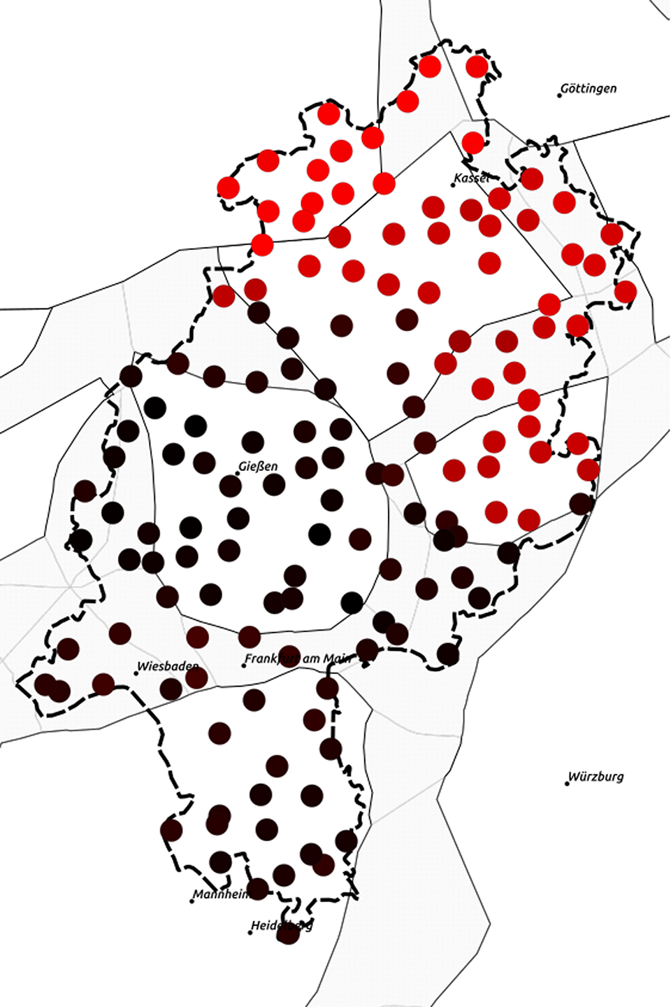
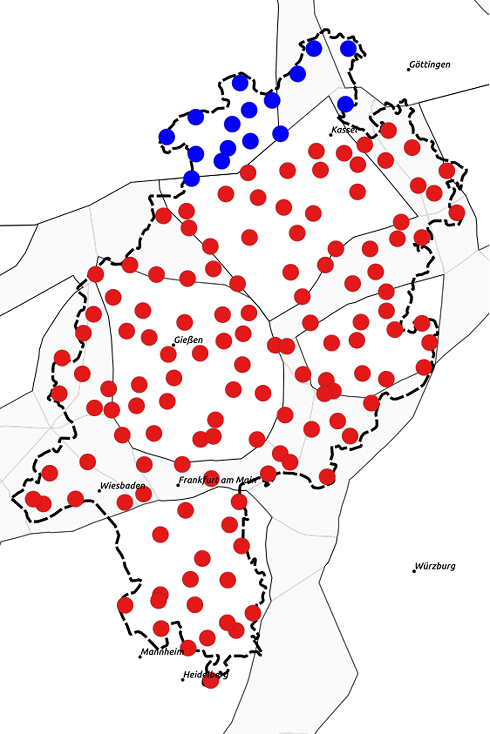
6.1 Comparing character n-grams and syntax
The results emerging from the MDS measurements for the n-gram and the syntax data are presented here in synopsis. However, different from Maps 4 and 12, now we use polygons instead of point symbols for ease of comparison. When comparing the resulting Maps 20 and 21, we notice that the n-gram data (Map 20), as just discussed, confirm the dialect classification of Wiesinger (Reference Wiesinger, Werner, Ulrich, Wolfgang and Herbert Ernst1983), whereas the syntax data (Map 21) show remarkably different areal structures. Only East Hessian behaves similarly in both datasets, although the respective red area extends somewhat more to the north in the n-gram data. In the syntax data, the border between Low German and North Hessian disappears, and we also notice similarities between dialects in the midwest and northwest of Hesse absent in the n-gram data (see the blueish areas in Map 21). While Central Hessian comes out very clearly in the n-gram data, for the syntactic data the same area seems to be more of a transition zone. Finally, a southern, primarily Rhine Franconian area can be discerned in both datasets, but in the n-gram data it is more uniform, especially in the area around Frankfurt, and extends more to the west.
MDS: SyHD trigram data (polygon map).

MDS: SyHD annotated syntax data (polygon map).
Given that character n-grams contain mostly phonological information, we can say that syntax differs from phonology to a fair extent. We find a correlation of 0.61 between the n-gram data and the syntax data, which is somewhat lower than in similar studies on Dutch (see Spruit, Heeringa, & Nerbonne, Reference Spruit, Wilbert and John2009:1636: 0.65 for Levenshtein distance versus syntactic variables) and on Swiss German (see Scherrer & Stoeckle, Reference Scherrer and Philipp2016:110: 0.66 for phonology versus syntax and 0.69 for morphology versus syntax). As discussed in section 5, it is safe to assume that the trigram data contain a high amount of phonological information insofar as they confirm established dialect areas that are defined according to phonological developments. In conclusion, then, for the dialects of Hesse, we can state that syntactic areas do not correspond to the traditional (primarily phonologically defined) dialect groups.
Apart from the question of whether syntactic correspond to other areas, there is a discussion on the nature of syntactic areal variation in comparison to other linguistic levels (see, for example, Fleischer, Reference Fleischer, Jürgen Erich and Joachim2019:655 and references cited therein). For our SyHD data, in addition to the fact that the emerging phonological and syntactic areas do not match in many respects, we also observe a difference in quality. As can be learned from a comparison, the spatial distributions in Map 20, showing the trigram data, are more clear-cut than in Map 21, showing the syntax data. For the latter, although there are clear areal patterns to discern, in many instances a somewhat more checkered picture with neighboring polygons of quite different hues and relatively distant polygons of very similar hues is the norm on a smaller scale. Similarly, the k-medoids cluster analysis revealed a greater number of locations with a very low silhouette width in the syntax data, indicating an unsure classification, as becomes clear from a comparison of Map 11 (syntax data, with many unsure locations in the southern North Hessian, Central Hessian, and western Rhine Franconian area) with Map 18 (trigram data, six-cluster solution, no unsure locations) and Map 19 (trigram data, five-cluster solution, a few unsure locations in areas traditionally viewed as transitional zones). In linguistic terms, this means that syntax is more prone to nonareal variation. Similar syntactic distributions are, to some extent, areally discontinuous. In contrast, the choice between phonological variants seems to be more of a categorial nature.
From a methodological point of view, it is important to stress that our results have been obtained by using data from the same project and the same informants, as opposed to the results reported in Spruit et al. (Reference Spruit, Wilbert and John2009) and Scherrer and Stoeckle (Reference Scherrer and Philipp2016), who used data from different atlas projects to compare syntactic and other phenomena. This leaves some doubt whether the reported differences between syntax and other linguistic levels are due to the linguistic levels as such or to differences in method or in the date of the surveys (with the syntactic surveys being considerably younger). In contrast, in our study, we can be sure that the very same persons produce different patterns in their syntax and trigram data.
6.2 Comparing dialect and standard
In the discussion of the syntax data, we noted that syntactically, Low German and North Hessian seem to be very similar. Further, these two dialect groups share many features that correspond to Standard German (see section 4.3). This raises the question of whether the dialects in northern Hesse are more Standard German-like than in the south. As a matter of fact, already the Hessian Dialect Census in the 1980s showed that dialects are receding most dramatically in northern and neighboring central Hesse (see Friebertshäuser & Dingeldein, Reference Friebertshäuser and Dingeldein1989: map 1). At the beginning of the twenty-first century, with (regional variants of) Standard German pervasive in most communicative situations, SyHD informants from the Low German area are very pessimistic about the future of their native dialect (see Birkenes & Fleischer, Reference Birkenes and Jürg2020:34–36).
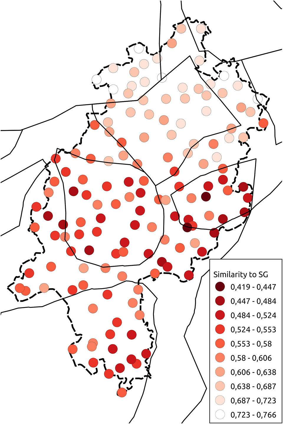
For both the syntax and n-gram data, we looked at the similarity to Standard German. For the syntax data, we emulated answers to all questions analyzed here with Standard German responses and compared these to the actual SyHD data. In the case of n-grams, we compared the similarity to the Standard German stimulus sentences. The results are presented as maps showing the cosine similarity between one location and Standard German. The similarity values were grouped into ten groups using Jenks natural breaks and mapped to a red-white color ramp. The redder a location is, the further it is from Standard German.
In the case of the n-gram data (Map 22), we notice that the dialects in the south and in the northeast show the most resemblance to Standard German, whereas the central and northwest dialects are furthest away. Low German, for example, is clearly distinct from Standard German, and so are the southern parts of North Hessian. We notice that the urban areas around Frankfurt/Wiesbaden and Kassel are the areas with the greatest similarities to Standard German. When looking at the syntax data (Map 23), we see a north-south divide, which is not present in the n-gram data. Here, the clearest similarities to Standard German are found in Low German and North Hessian (i.e., also in areas fairly distinct from Standard German from the perspective of the n-grams). Note that while a natural interpretation for the syntax data could be that they simply show Standard German structures finding their way into the local dialects, which are known to recede in favor of varieties close to Standard German, the n-gram data show that this is not the case on a more general level. Still, it could hold for syntax.
Similarity to Standard German (n-grams).
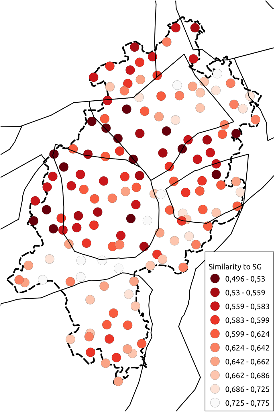
Similarity to Standard German (syntax).
For the syntax data, in some instances it is likely that Low German and North Hessian being close to Standard German in the SyHD data is a relatively young state of affairs. This will be discussed with respect to the five features defining the Low German plus North Hessian cluster according to Table 4. With respect to the first feature, pronominal partitivity, where the partitive use of welch- is thought to have its origin in the north of the German-speaking area (see Fleischer, Reference Fleischer, Jürgen Erich and Joachim2019:644), sources from the 1920s, namely Martin (Reference Martin1925:92) and Soost (Reference Soost1920:200–01), still document the “partitive particles” for a Low German and a North Hessian local dialect, respectively, although one can deduce from the descriptions that they are receding. In the twenty-first century SyHD data, “partitive particles” are almost completely absent in the north, where welch- dominates (see Birkenes & Fleischer, Reference Birkenes and Jürg2020:44). As to the pronominal adverb, here the unsplit variant (davon) emerges as typical for North Hessian and Low German in the SyHD data. Unsplit pronominal adverbs are the only construction also licensed in Standard German, while the split construction (da weiß ich nichts von) is usually thought to be typical for Low German and adjacent Central German areas (see Fleischer, Reference Fleischer2017; Fleischer, Reference Fleischer, Jürgen Erich and Joachim2019:646–47). This is not directly reflected in the SyHD database (note, however, that the split construction is indeed attested in the North Hessian and Low German dialects, as discussed by Fleischer, Reference Fleischer2017:513–15; however, the unsplit pronominal adverb is more frequent). As to the serialization of object pronouns, the preference for the serialization of direct before indirect object found in the north is also the serialization preferred in Standard German (see Fleischer, Reference Fleischer, Jürgen Erich and Joachim2019:646). However, in this case, at least for Low German this might be an old trait, as the serialization of direct before indirect object is also typical for older stages of Low German, but less so for older stages of High German (see Fleischer, Reference Fleischer2013). Thus, in this case it is not clear whether the correspondence with Standard German is due to recent Standard German influence or much older. For the periphrastic subjunctive, we are in a better position to assess the situation, as there exists a grammatical description from 1920. Periphrastic täte in subjunctive contexts seems to be untypical for Low German (see Fleischer, Reference Fleischer, Jürgen Erich and Joachim2019:641 with references cited therein), which corresponds to the SyHD data. However, periphrastic täte is described for a North Hessian local dialect in 1920 (see Soost, Reference Soost1920:182–83), but in the SyHD data würde dominates in the respective area (see Birkenes & Fleischer, Reference Birkenes and Jürg2020:45). Thus, here the respective North Hessian dialects seem to have changed in the direction of Standard German. Finally, for the fifth defining feature according to Table 4, the situation is quite different. Neuter agreement forms for female persons is a feature totally absent from Standard German. Here, therefore, there can be no question about Standard German influence.
In summary, the situation is not that clear. Some syntactic phenomena that are typical for twenty-first century North Hessian and Hessian Low German might indeed be due to recent Standard German influence, but for others, this is doubtful or clearly not the case (see Birkenes & Fleischer, Reference Birkenes and Jürg2020:43–46 for a more detailed discussion). Some, though not all, of the resemblance to Standard German in this area might be old, and even in this northern area, which generally features close resemblances to Standard German, there are prominent syntactic features that do not correspond to Standard German.
7. Conclusions and outlook
This paper has shown that the geography of syntactic structures is different from that of phonology (provided our assumption that phonology is represented in a dominant way in character trigrams is correct). Different from earlier dialectometrical studies on the same issue, we could exclude that the differences observed are due to method or sampling by using the very same dataset (or, more precisely, a dataset and a subset thereof) for both the syntax and trigram data, thus avoiding that differences in the data elicitation or the age of the data are responsible for differences.Footnote 16 It turned out that while the syntax data do show spatially structured patterns, not only do the emerging areas diverge to a considerable extent from the trigram data, but also the nature of the respective areal patterns is different. This finding is in line with Kortmann’s (Reference Kortmann, Peter and Jürgen Erich2010:846) claim that syntactic variation is, among other things, “less salient, less categorical, and in many cases a matter of statistical frequency rather than the presence or absence of a feature […].” For future research, it remains to be seen whether our central finding can be corroborated for other regions. If it turns out that this is the case, then we could establish that in terms of dialect geography, syntax behaves differently.
Acknowledgments
The present paper takes a new perspective on data that have been collected in the project “Syntax hessischer Dialekte” (SyHD, 2010–2016, principal investigators: Jürg Fleischer, Alexandra N. Lenz, Helmut Weiß), funded by two subsequent grants of the Deutsche Forschungsgemeinschaft DFG (FL 702/2-1, FL 702/2-2), which are gratefully acknowledged hereby. For feedback, suggestions, and various other kinds of help we are grateful to an anonymous reviewer, Ludwig M. Breuer, Katja Daube, Robert Engsterhold, Sara K. Hayden, Alfred Lameli, Jeffrey A. Pheiff, Lea Schäfer, Oliver Schallert, Yves Scherrer, Jürgen Erich Schmidt, and especially Michael Cysouw. Sara K. Hayden also significantly improved our English. As usual, all errors are ours.


 Open access